CHEM 112 A04&09 GENERAL CHEMISTRY II … · the structures of different organic molecules and obtain ... For the aprotic liquids, ... determination of evaporation rate as the independent

CHEM 112 A04&09

GENERAL CHEMISTRY II

LABORATORY REPORTS

SPRING 2017

General Chemistry II Lab Reports Class Portfolio

Spring 2017• Volume 1, Issue 2

Lab

No.

Title Author Page

No.

1 Calculated Structures of Organic

Molecules

Amanda Malooley 3-7

2 Connecting Molecular Structure to

Evaporation Rate

Cathleen Bressers 8-14

3 Analysis of Dyes and Mixtures Using

Spectrophotometry

Emily Walker 15-19

4 Kinetics Kaitlyn R.

Yablonski

20-26

5 Equilibrium experiment group:

LeChatelier’s Principle and

Determination of Kc – Ka of a

chemical indicator

Mariana

Valenzuela

27-32

6 Equilibrium #1 and Equilibrium #2 Chloe Frye 33-36

7 Dissociation of Acetic Acid and

Acetate and the Molecular Structure

and Acid Strength

Logan Felton 37-44

2

TABLE OF CONTENT

CHEM 112 SPRING 2017, 1(2), 3-7

CHEM 112 GENERAL CHEMISTRY

LABORATORY SPRING 2017

Indiana University of Pennsylvania

Calculated Structures of Organic Molecules

Amanda Malooley

Department of Biology, Indiana University of Pennsylvania, Indiana, PA 15705

Academic Editor: H. Tang

Received: May 6, 2017 / Accepted: May 13, 2017 / Published: May 22, 2017

Abstract: This lab primarily focused on mapping out the structure of organic compounds on WebMO, to see how the molecule’s bond length, angle, electrostatic constant, and dipole moment affect boiling point. Boiling point indicates how strong the bonds within the molecule are. Creating the structure in WebMO, which calculates the geometry optimization, gives the values needed to determine and confirm the polarity and gives way to view how the molecule most likely is structured. The results showed that dipole moment and boiling point have a direct relationship for protic and aprotic liquids. The results also showed that dielectric constant and boiling point have a direct relationship for both protic and aprotic liquids. Based on the graphed data, the dielectric constant shows a better correlation to boiling point than does dipole moment.

1. Introduction and Scope

Organic compounds are defined as compounds that contain carbon. They are found in items such as alcohol, water, and many other common items. Although all organic compounds contain carbon, they all differ through the combination of atoms and structures. The bonds between atoms in the molecule heavily influence the structure of a molecule. One way to determine the strength of the bonds within a molecule is through mapping out the structure through software like WebMO. The purpose of this lab was to map out the structures of different organic molecules and obtain measurements: bond angle, bond length, and dipole moment. The measurements were to be compared to the boiling point and electrostatic constant of

OPEN ACCESS

CHEM 112 SPRING 2017, 1(2), 3-7 4

each molecule to determine if there is a relationship between the bond and the boiling point and electrostatic constant.

2. Experimental Procedure

The experiment was sectioned off into 2 parts: molecular shapes/ bond angles and organic functional groups. The first portion had to be drawn since the manual only gives the condensed version of the compounds. The first set was drawn using WebMO software, which calculates bond length, bond angle, and dipole moment. All three calculations were recorded for each molecule. The same procedure was followed for the second set of molecules, except that the condensed structure was given.

3. Results and Calculations

Table 1. Formula, Lewis Structure, Molecular Shape, and Bond Angle of 6 different molecules. Formula Molecular Shape Bond Angle

HCN Linear 180 NOF Bent 110.37

OCH2 Trigonal Planar 122.16

H2O Bent 105.49

NH3 Trigonal Pyramid 107.18

CH4 Tetrahedral 109.47 Table 2. The formula, drawing, functional group, dipole moment, bond distance and bond angle of aprotic and protic liquids

Aprotic Liquids Formula Functional Groups

Dipole Moment (Debye)

Bond Distance (A)

Bond Angle(s)

Acetone (propan-2-one)

(CH3)2CO Keytone 3.12 CC:1.51 C-O:1.28

116.63

Propanal CH3CH2CHO Aldehyde 3.02 C-C:1.51 O-C:1.19

113.59

Ethyl methyl ether (methoxyethane)

(CH3)2CH2O Ether 1.35 O-C:1.39 C-C:1.52

114.23

Nitromethane CH3NO2 Nitro 4.02 N-O:1.19 N-C:1.48

125.78

Butane (CH3)2(CH2)2 0.00 C-C:1.53 113.07 Protic Liquids Formula Functional

Groups Dipole

Moment (Debye)

Bond Distance (A)

Bond Angles

(Degre

CHEM 112 SPRING 2017, 1(2), 3-7 5

es)

Propyl alcohol (propan-1-ol)

CH3(CH2)2OH

Alcohol 1.65 C-C:1.52 C-O:1.40

116.63

Isopropyl alcohol (propan-2-ol)

(CH3)2CHOH Alcohol 1.71 C-C:1.53 C-O:1.41

110.94

Propylamine (propan-1-amine)

CH3(CH2)2NH2

Amine 1.40 C-N:1.46 C-C:1.52

112.88 110.66

Isopropyl amine (propan-2-amine)

(CH3)2CHNH2

Amine 1.39 C-C:1.53 C-N:1.46

111.49 108.82

Figure 1. This graph displays the relationship between boiling point (K) and dielectric constant of the aprotic liquids.

y = 0.3214x - 84.676 R² = 0.995112079

0 0.5

1 1.5

2 2.5

3 3.5

4 4.5

5

250 270 290 310 330 350 370 390

Diel

ectr

ic C

onst

ant

Boiling Point (K)

Boiling Point and Dipole Moment of Aprotic Liquids

CHEM 112 SPRING 2017, 1(2), 3-7 6

Figure 2. This graph displays the relationship between boiling point(K) and dipole moment (Debye) of aprotic liquids. For the aprotic liquids, the R-squared value is closer to 1 in Figure 2, which is the boiling point

compared with dielectric constant. Therefore, the correlation is higher between boiling point and dielectric constant than the correlation between boiling point and dipole moment.

Figure 3. The relationship between boiling point (K) and dielectric constant for protic liquids.

y = 0.0377x - 9.6033 R² = 0.944420783

0

5

10

15

20

25

30

35

40

250 270 290 310 330 350 370 390

Dipo

le M

omen

t (De

bye)

Boiling Point (K)

Boiling Point and Dielectric Constant of Aprotic Liquids

y = 0.2465x - 70.326 R² =0.992659565

0

5

10

15

20

25

250 270 290 310 330 350 370 390

Diel

ectr

ic C

onst

ant

Boiling Point (K)

Boiling Point and Dielectric Constant of Protic Liquids

CHEM 112 SPRING 2017, 1(2), 3-7 7

Figure 4. The relationship between boiling point (K) and dipole moment (debye) for protic liquids. For the protic liquids, the R-squared value in Figure 3 was closer to 1 than the R-squared value in

Figure 4. The correlation was higher between dielectric constant and boiling point than dipole moment and boiling point.

4. Summary and Discussion

Based on the recorded and graphed data, dielectric constant is a better indicator of boiling point than dipole moment. Although the correlation between boiling point and dipole moment were positive, the R-squared value for the graphs displaying dielectric constant with boiling point were closer to 1. Dielectric constant can be tested and calculated using a liquid sample, whereas dipole moment is a function of magnitude that is calculated.

Acknowledgments

The author gratefully acknowledges his lab partner Adaysha Spence for her assistance in performing the experiment and all other aspects of the process, including data collection, statistical calculations, and lab clean-up to enumerate a few.

© 2017 by the author. This article is an open access article.

y = 0.005x - 0.1475 R² =0.93818623

0

0.2

0.4

0.6

0.8

1

1.2

1.4

1.6

1.8

250 270 290 310 330 350 370 390

Dipo

le M

omen

t (De

bye)

Boiling Point (K)

Boiling Point and Dipole Moment of Protic Liquids

CHEM 112 SPRING 2017, 1(2), 8-14




Connecting Molecular Structure to Evaporation Rate

Cathleen Bressers



Received: February 6, 2017 / Accepted: May 13, 2017 / Published: May 22, 2017

Abstract: In this experiment, we use a simple temperature change experiment and WebMO Software to investigate and analyze the relationship between intermolecular forces and molecular structure. In Part I, we experimentally determine the evaporation rate of four alcohols (methanol, ethanol, 1-propanol, and 1-butanol) and two other organic liquids (acetone, pentane). In Part II, our analysis involves computer-driven (WebMO) calculations of the molar mass, dipole moment, and the oxygen electrostatic partial charge. We compare these three values from our calculations, along with known values for the dielectric constant with the experimentally determined evaporation rate to investigate how molecular structure affects the evaporation rate, and by proxy, the intermolecular forces. Our analysis indicates that the oxygen electrostatic partial charge is the most significant characteristic in determining the strength of intermolecular forces in alcohols, due to the increase in strength of hydrogen bonding. Our results also indicate a weaker relationship between polarity (as indicated by dipole moment and the dielectric constant) and the strength of intermolecular forces. The evaporation rate is much slower for the alcohols (which can participate in hydrogen bonds) than for both acetone and pentane.


This lab has four main purposes: (1) using chemistry software to calculate the molecular properties of a selection of simple molecules, (2) use the rate of temperature change to calculate evaporation rate, (3) comparing characteristics of four alcohols and two other organic compounds, and (4) identifying the

OPEN ACCESS

CHEM 112 SPRING 2017, 1(2), 8-14 9

relationships between evaporation rate, intermolecular forces, and characteristics of molecular structure. The lab serves as a continuation of our exploration of molecular forces, using an experimental determination of evaporation rate as the independent variable in our analysis. We concentrate our analysis on four alcohols (methanol, ethanol, 1-propanol, and 1-butanol) and two other organic liquids (acetone, pentane).

We accomplish our objectives in this lab in two parts. In Part I, we experimentally determine the evaporation rate which is central to our analysis (procedure described in Section 2). In Part II, we utilize the WebMO program to calculate several additional values based on molecular structure. We then perform data analysis by identifying the direction and strength of linear relationships between a few characteristics of molecular structure (molar mass, dipole moment, dielectric moment and electrostatic partial charge on oxygen) and the evaporation rate. The goal of this analysis is to garner (1) an understanding of the effects of the hydroxyl (-OH) functional group on the strength of intermolecular forces in organic compounds (using evaporation rate as a proxy), (2) identifying which molecular characteristic has the greatest impact on the strength of intermolecular forces and (3) comparing our experimental analysis with theoretical expectations.


Part I, Evaporation Rate: In this experiment, we use small samples of each liquid placed in a test tube. We wrapped equal sized

strips of paper towel around a temperature probe, inserted the probe in each test tube for one minute to allow saturation and equilibrium, and then allow the paper towel to air dry for roughly 30 seconds. The temperature probe is connected to the computer and temperature data is collected at a rate of 0.5s. The temperature change data forms a cooling curve. We determine a linear best fit for this data and record the slope as the rate of evaporation. We repeat this process for each of the six organic liquids and record the results.

Part II, Structure Calculations: In the second part of our experiment, we construct a 3D model of the molecule in the WebMO software

for each of our six compounds. Using the “6-31G* basis set for HF Geometry Optimization, we calculate and record the molar mass, dipole moment and oxygen partial change (where applicable) for each molecule. Using the calculated values from WebMO and the experimental values, we conduct some basic data analysis (Section 3).


Part I & II Data Table:

CHEM 112 SPRING 2017, 1(2), 8-14 10

Compound Formula Molar Mass (g/mol)

Dielectric Constant


Oxygen Partial Charge

Evaporation Rate (°C/s)

methanol CH3OH 32.02 32.6 1.8667564574 -0.726 -0.1444 ethanol CH3CH2OH 46.07 24.3 1.7381497696 -0.735 -0.1284

1-propanol CH3CH2CH2OH 60.10 20.1 1.6488603557 -0.742 -0.02286 1-butanol CH₃CH2CH2CH2OH 74.12 17.8 1.6947266235 -0.743 -0.01449 acetone (CH3)2CO 58.08 20.7 3.0733095163 -0.516 -0.2757 pentane CH3CH2CH2CH2CH3 72.15 1.8 0.0663533058 ——— -0.4262

Graphical Analysis:

Figure 1: Evaporation Rate vs Molar Mass: The low R² value indicates the lack of a strong linear relationship.

R² = 0.0244

-0.5

-0.4

-0.3

-0.2

-0.1

0

30.00 40.00 50.00 60.00 70.00 80.00

Evap

orat

ion

Rat

e (°

C/s

)

Molar Mass (g/mol)

Evaporation Rate vs Molar Mass

CHEM 112 SPRING 2017, 1(2), 8-14 11

Figure 2: Evaporation Rate vs Dipole Moment: The R² value is quite low, but the data indicates a very weak positive linear relationship. The relationship between polarity and evaporation rate is more evident in Figure 3.

Figure 3: Evaporation vs Dielectric Constant: There is a weak positive linear relationship between the evaporation rate and dielectric constant, indicating that as polarity increases, the magnitude of the evaporation rate decreases.

R² = 0.1282

-0.5

-0.4

-0.3

-0.2

-0.1

0

0.00 0.50 1.00 1.50 2.00 2.50 3.00 3.50

Evap

orat

ion

Rat

e (°

C/s

)


Evaporation Rate vs Dipole Moment

R² = 0.3545

-0.5

-0.4

-0.3

-0.2

-0.1

0

0 5 10 15 20 25 30 35

Evap

orat

ion

Rat

e (°

C/s

)

Dielectric Constant

Evaporation vs Dielectric Constant

CHEM 112 SPRING 2017, 1(2), 8-14 12

Figure 4: Evaporation Rate vs Oxygen Partial Charge: There is a strong negative linear relationship between the evaporation rate and dielectric constant, indicating that and increase the magnitude of the partial charge on the oxygen atom correlates with an decrease in the magnitude of the evaporation rate.


Summary of Results:

The magnitude of the evaporation rate amongst the alcohols (methanol, ethanol, 1-promanol, 1-butanol) decreases as the number of CH2 groups increases. For the other compounds involved in this experiment (acetone and pentane), the magnitude of the evaporation rate is significantly higher than for any of the alcohols. Amongst the relationships tested, only the evaporation rate versus oxygen partial charge shows a strong linear relationship, with an R² value of 0.748. The next best fit is dielectric constant at 0.3545. Dipole moment and the dielectric constant show a positive relationship with evaporation rate—the slower the magnitude of the evaporation rate, the higher the polarity of the molecule. The oxygen partial charge and the molar mass show a negative relationship with evaporation rate—the slower the magnitude of the evaporation rate, the smaller the molar mass and smaller the magnitude of the oxygen partial charge. These results indicate that the oxygen partial charge has a strong bearing on the evaporation rate. The stronger the electron density on the oxygen atom, the slower the magnitude of the evaporation rate. Additionally, the higher the polarity of the molecule, the slower the magnitude of the evaporation rate. The molar mass doesn’t seem to play a significant role, has a more complex (i.e. non-linear) relationship with the evaporation rate, or requires a greater breadth of compounds to acquire sufficient data.

R² = 0.748

-0.45

-0.35

-0.25

-0.15

-0.05

0.05

-0.8 -0.75 -0.7 -0.65 -0.6 -0.55 -0.5 -0.45

Evap

orat

ion

Rat

e (°

C/s

)

Oxygen Partial Charge

Evaporation Rate vs Oxygen Partial Charge

CHEM 112 SPRING 2017, 1(2), 8-14 13

Discussion:

1. All the molecules in this data set except pentane are polar (as indicated by non-zero values in the dipole moment and dielectric constant). Pentane is a hydrocarbon containing only C-C and C-H bonds and is therefore nonpolar and only subject to London forces. Due to polarity, all the other compounds are subject to London-forces and dipole-dipole forces. The alcohols (methanol, ethanol, 1-promanol, 1-butanol), by definition, all contain the hydroxyl group (-OH) and are therefore subject to hydrogen bonding as well. Acetone has an oxygen, but the oxygen does not have an attached hydrogen atom, and therefore is not subject to hydrogen bonding. Pentane has no functional groups and is therefore also not subject to hydrogen bonding.

2. The expected effects of molar mass on the magnitude of the evaporation rate indicate a negative relationship. The larger the molecule, more energy is required to change the state of the molecule from liquid to gas, and so the magnitude of the evaporation rate is slower. The dipole moment is also expected to have a negative relationship with the magnitude of the evaporation rate (positive with the signed rate). As the polarity increases, negative and positive ends of molecules in the liquid form dipole-dipole bonds and increase the amount of energy required to change the structure, resulting in slower evaporation. As the dielectric constant is also an indicator of polarity, the same logic and relationship is expected to exist. The charge on the oxygen atom indicates the electron density on the oxygen atom. As the magnitude of the charge increases, the oxygen is more likely to attract hydrogen atoms from nearby molecules. This increases the intermolecular forces, and thus decreases the evaporation rate. So, the magnitude of the charge and the magnitude of the evaporation rate have a negative relationship.

3. An increase in intermolecular forces should decrease the magnitude of the evaporation rate. As the strength of the bonds holding the molecules together increases, more energy is required to break these bonds and alter the state of the compound from liquid to gas.

4. The graphical relationships from this experiment largely support this idea. The dipole moment and dielectric constant (both measures of polarity) indicate a slowing of the evaporation rate (a higher value per Figures 2,3) as the polarity increases. The increase in polarity increases the dipole-dipole forces between molecules and thus supports the idea from 3. The partial charge on the oxygen shows a slowing of the evaporation rate as the magnitude of the charge increases (a lower value per Figure 4). The increase in the magnitude of oxygen partial charge increases the hydrogen bonding in the molecule, and is therefore also consistent with the expectation from 3. The molar mass shows the least significant contribution to the idea from 3. The relationship is incredibly weak. If you look at the graph and data closely, the alcohols do exhibit a positive linear trend while the other molecules exhibit a negative linear trend. The strength of these relationships is unknown, however indicate that the relationship in these graphs is complicated by more than just the molar mass of the molecules. For the alcohols, an increase in molar mass seems to decrease the evaporation rate as expected (see 2 for explanation), however for the non-alcohol compounds the opposite seems to be true. This may be due to the lack of hydrogen

CHEM 112 SPRING 2017, 1(2), 8-14 14

bonding in the other molecules, but there isn’t sufficient data to draw any concrete conclusion. 5. Based on our experiment, the partial charge on the oxygen seems to have the greatest effect in

determining the evaporation in alcohols. This is indicated by the R² value of 0.748, the strongest linear relationship amongst the groups. This indicates that the difference in degree of the London-forces and dipole-dipole forces between alcohols is less significant than the effects of hydrogen bonding (see 2 for more details on oxygen partial charge and intermolecular forces).

6. The evaporation rates of acetone and pentane are significantly greater (more negative) than the alcohols with similar molar masses. The magnitude of the evaporation rate for acetone is more than 1,100% higher than that of 1-propanol, the compound with the closest molecular mass. Pentane is 2,840% higher than 1-butanol. The primary difference between the alcohols and the other compounds is the ability of the compound to engage in hydrogen bonding. All of the alcohols are capable of forming hydrogen bonds due to the presence of the hydroxyl group, but acetone and pentane both lack a functional group that can form hydrogen bonds. Thus, compared to alcohols of similar molar mass, the intermolecular forces are much weaker, resulting in quicker evaporation.

Acknowledgments

The author gratefully acknowledges his lab partner Faith Dumm for his assistance in performing the experiment, data collection, and calculations.


CHEM 112 SPRING 2017, 1(2), 15-19




Analysis of Dyes and Mixtures Using Spectrophotometry

Emily Walker




Abstract: In our first spectrophotometry lab we examined solutions of dyes by using a spectrophotometer. Specifically, we were looking at solutions which were “clear”. “Clear” solutions are solutions that light can pass through. When light passes through a solution the light may pass through, be reflected, or be absorbed. In our lab we were focusing on the light being absorbed. We recorded the absorbance for each different concentration we had. In our second spectrophotometry lab we used a spectrophotometer to determine the absorbance of copper, nickel, and an unknown coin using different wavelengths. Once we determined the absorbance we were able to figure out the concentration for these metals.


The purpose of our first lab was to determine the absorbance of one solution with various concentrations. We did this by observing a “clear” solution in a spectrophotometer. We then used LoggerPro to determine our values by using the maximum wavelength and recording the absorbance at that value for each trial. Additionally, we needed determine the concentration of our unknown. In our second spectrophotometry lab, the purpose was to use a spectrophotometer to determine the absorbance values of copper, nickel, and an unknown coin. We determined this information by using LoggerPro to record the absorbance values at various wavelengths. We then used these absorbance values to determine the concentration. Furthermore, we used our concentration to determine our x and y values.

OPEN ACCESS

CHEM 112 SPRING 2017, 1(2), 15-19 16

The scope of this paper is to determine the concentration of an unknown, as well as absorbance values for various metals through the use of a spectrophotometer. This information can aid in determining what material you may be working with based on the values given.

2. Experimental Procedure for Determining the Concentration of an Unknown

This lab required test tubes, beakers, cuvettes, distilled water, graduated cylinders, a scale, a spectrophotometer, and LoggerPro. In our first spectrophotometry lab we were required to create five solutions. We used a stock solution to create our five different solutions. We began with a solution with 10% concentration by diluting the stock solution. In order to make a 10% concentration we added nine milliliters distilled water and one milliliter of the stock solution. From there, we made the rest of our solutions. We made solutions with 10%, 20%, 30%, 40%, and 50% concentrations. In addition, we had an unknown solution. Once our solutions were made we transferred them into cuvettes, in order to be read in the spectrophotometer. We then recorded the wavelengths of maximum absorbance. In our second spectrophotometry lab we needed to prepare our solutions. We began by weighing out our salt, and then adding distilled water. We filled our cuvettes with our mixed solution, and used our spectrophotometer to record our results. Once we had our results, we plotted our results to determine the relationship between absorbance and concentration.


Lab #1 table: Concentration Make up of solution Absorbance 10% 1mL of solution+ 9mL

distilled water 0.148

20% 2mL of solution + 8 mL distilled water

0.188

30% 3 mL of solution + 7 mL distilled water

0.204


0.256


0.550

Unknown Unknown 0.083

CHEM 112 SPRING 2017, 1(2), 15-19 17

First lab Absorbance vs. Concentration graph:

Looking at our graph, we can see that our R2 value was very small. This is a problem because it shows

that our data was not valid and that we must have had error in our experiment. Lab #1 calculations: X = unknown concentrations Y = 0.872x + 0.0076 0.083 = 0.872 x + 0.0076 X = 0.086468 approximately 8.6%

Lab #2 table:

Wavelength A coin A Cu A Ni A Cu/ A Ni A Coin/ A Ni 610 0.075 0.077 0.235 0.328 0.319 620 0.097 0.114 0.276 0.413 0.351 630 0.119 0.167 0.327 0.511 0.364 640 0.149 0.219 0.371 0.590 0.402 650 0.183 0.290 0.411 0.706 0.445 660 0.217 0.360 0.422 0.853 0.514 670 0.260 0.447 0.421 1.06 0.618 680 0.300 0.542 0.428 1.27 0.701 690 0.346 0.637 0.443 1.44 0.781 700 0.397 0.750 0.460 1.63 0.863

R² = 0.7272

y = 0.872x + 0.0076

0

0.1

0.2

0.3

0.4

0.5

0.6

0 0.1 0.2 0.3 0.4 0.5 0.6

Abso

rban

ce (c

m-1

)

Concentration (%)

Absorbance vs. Concentration

CHEM 112 SPRING 2017, 1(2), 15-19 18

Second lab graph:

Lab #2 calculations: Y = A coin/ A Ni = 0.075/ 0.235 = 0.319 X = A Cu / A Ni = 0.077/0.235 = 0.328 Mcu/ Mcustd = 0.4433 Mcu/0.117 = 0.4433 Mcu = 0.117 (0.443) Mcu = 0.519 Error Analysis In our first spectrophotometry lab, we had a very small R2 value. This shows us that we had an error in our first lab. Our error could be due to not having the correct concentration for each of our samples. We must have made a human error in this lab, but we were more cautious and avoided error in our second lab. In our second lab, we had an accurate R2 value, therefore, we knew that we did not make as much error as we did in our first lab.


Based on the analytical wavelength and the color wheel, the color absorbed in our first lab was blue. This makes sense because our analytical wavelength was in the orange on the color spectrum, and in order to

y = 2.2287x - 0.2989 R² = 0.9996

0

0.2

0.4

0.6

0.8

1

1.2

1.4

1.6

1.8

0 0.1 0.2 0.3 0.4 0.5 0.6 0.7 0.8 0.9 1

Abso

rban

ce o

f Coi

n/ A

bsor

banc

e of

Ni

Absorbance of Cu/ Absorbance of Ni

Absorbance of Cu/ Absorbance of Ni vs. Absorbance of Coin/ Absorbance of Ni

CHEM 112 SPRING 2017, 1(2), 15-19 19

find the color absorbed you look at what is opposite that color on the color wheel. The color opposite of orange on the color wheel is blue. We were able to collect our data by using a spectrophotometer for each of our concentrations. We used our data that we collected to observe the relationship between absorbance and concentration. Although we had an error in this lab, we were able to use our data in order to form a conclusion. In our second lab we had an accurate R2 value, and therefore were able to determine the relationships between the metals that we observed.

Acknowledgments

The author gratefully acknowledges her lab partner Jacob Lewis for his assistance in completing this lab. Jacob assisted in performing the lab, calculating our results, and determining what our results represented.


CHEM 112 SPRING 2017, 1(2), 20-26 20

CHEM 112

GENERAL CHEMISTRY LABORATORY

SPRING 2017 Indiana University of Pennsylvania

Kinetics

Kaitlyn R. Yablonski

Department of Biology, Indiana University of Pennsylvania, Indiana PA 15705March 22, 2017



Abstract: In the two Kinetics labs (Lab 1 and Lab 2) we familiarized ourselves with

the rate law. The rate law is a measure of time over which a chemical reaction takes

place. For the first lab we used the method of initial rates, and for the second lab we

used the graphical analysis method. The initial rates method requires experimental

data, so we had to run a series of experiments and collect data before we could

actually use the rate law to find our unknown values. For the second experiment, we

were given the rate law, and we had to find the reaction order.

1. Introduction

In the first lab we were supposed to determine the rate of the chemical reaction taking place

in our experiments. We used the rate law and data we collected to determine the rate, since the

orders can only be determined experimentally. In the second lab we had to find a hypothetical,

cost-effective and environmentally-friendly method for decomposing hydrogen peroxide with the

help of a catalyst. To do this, we again ran experiments and used LoggerPro to collect our data.

We then put this data into 3 different plots to determine which method was the best using

graphical analysis.

OPEN ACCESS

CHEM 112 SPRING 2017, 1(2), 20-26 21

2. Procedure

Haley and I shared equally in the responsibilities for both labs, and Amanda helped a lot with

the calculations for the second lab, especially when Haley and I were confused.

Lab 1:

For lab one we began by running our experiments and collecting data. To do this, we

combined various combinations of KIO3, NaHSO3, and water. We collected data such as the

final concentrations, the temperature after mixing, the time it took for the reaction to complete,

the reaction rate, and the average reaction rate. We put all of this into a table, and ran the

experiment 4 times with 2 trials each. After we attained all our numbers, we were then able to

use the equation for reaction rate (R=k[A]a[B]b) to determine the order of the reaction and the

unknown values: a, b, and the activation energy.

Lab 2:

For the second lab we ran two experiments that involved a pressure collection setup, H2O, KI,

and H2O2. We first combined the H2O2 and H2O in a flask. Then we attached a stopper, a

pressure sensor, and a syringe with the KI in it. We set the pressure using a machine before

attaching the set-up to the computer and using LoggerPro. We would begin the experiment by

adding the syringe of KI to the solution and beginning the collection of data on LoggerPro. We

ran the experiment for 300 seconds. We had to do this twice with 2 different sets of given

volumes of the reactants. Unfortunately, our group was not able to collect ‘good’ data for the

second experiment, so we had to share data with another group. Then we put the data from the

first experiment into three graphs: time vs. concentration, time vs. 1/concentration, and time vs.

lnConcentration. We did the same style of graphs for the second set of data as well. Using our

graphs, we were able to look at the trend lines and the y-intercept equation to determine the order

of the reaction.

CHEM 112 SPRING 2017, 1(2), 20-26 22


Lab 1:

Average Rates:

1. (0.022+0.016)/2 = 0.019

2. (0.071+0.071)/2 = 0.071

3. (0.059+0.040)/2 = 0.0495

4. (0.0098+0.0095)/2 = 0.0097

Rate Order:

Reaction Rate = k[A]a [B]b

a = ln (R1/R3) / ln (A1/A3) a = ln (0.019/0.0495) / ln (0.005/0.010) = 1.4 ~ 1

b = ln (R1/R2) / ln (B1/B2)b = ln (0.019/0.071) / ln (0.004/0.008) = 1.9 ~ 2(supposed to be 1.)

Activation Energy = ln(R1/R4) = Ea/0.00831 Kj/mol K * (1/291.3K – 1/323K) = 16.6

Exper-iment

Trial Va of 0.025 M KIO3

VB of 0.020 M NaHSO3

VH2O [A] [B] Temp (ºC)

Time (s)

Reaction Rate (1/s)

Average Rate (1/s)

1 1 10 10 30 0.005 0.004 25.2 45 0.022 0.019 2 24.8 60 0.016

2 1 10 20 20 0.005 0.008 24.2 14 0.071 0.071 2 24.2 14 0.071

3 1 20 10 20 0.010 0.004 24.2 17 0.059 0.0495 2 24.5 25 0.040

4 1 10 10 30 0.005 0.004 18.4 102 0.0098 0.0097 2 18.2 105 0.0095

CHEM 112 SPRING 2017, 1(2), 20-26 23

Lab 2: First Test

0 0.1 0.2 0.3 0.4 0.5 0.6 0.7 0.8 0.9

1

0 0.2 0.4 0.6 0.8 1

Conc

entr

atio

n (m

ol/L

)

Time (s)

Time vs Concentration

0 0.1 0.2 0.3 0.4 0.5 0.6 0.7 0.8 0.9

1

0 0.2 0.4 0.6 0.8 1

1/Co

ncen

trat

ion

Time (s)

Time vs 1/Concentration

0 0.1 0.2 0.3 0.4 0.5 0.6 0.7 0.8 0.9

1

0 0.2 0.4 0.6 0.8 1

lnCo

ncen

trat

ion

Time (s)

Time vs lnC

CHEM 112 SPRING 2017, 1(2), 20-26 24

Second Test

0

0.1 0.2 0.3 0.4 0.5 0.6 0.7 0.8 0.9

1

0 0.2 0.4 0.6 0.8 1

1/co

ncen

trat

ion

Time (s)

Time vs 1/C

0 0.1 0.2 0.3 0.4 0.5 0.6 0.7 0.8 0.9

1

0 0.2 0.4 0.6 0.8 1

lnCo

ncen

trat

ion

Time (s)

Time vs lnC

0 0.1 0.2 0.3 0.4 0.5 0.6 0.7 0.8 0.9

1

0 0.2 0.4 0.6 0.8 1

Conc

entr

atio

n (m

ol/L

)

Time (s)

Time vs Concentration

CHEM 112 SPRING 2017, 1(2), 20-26 25

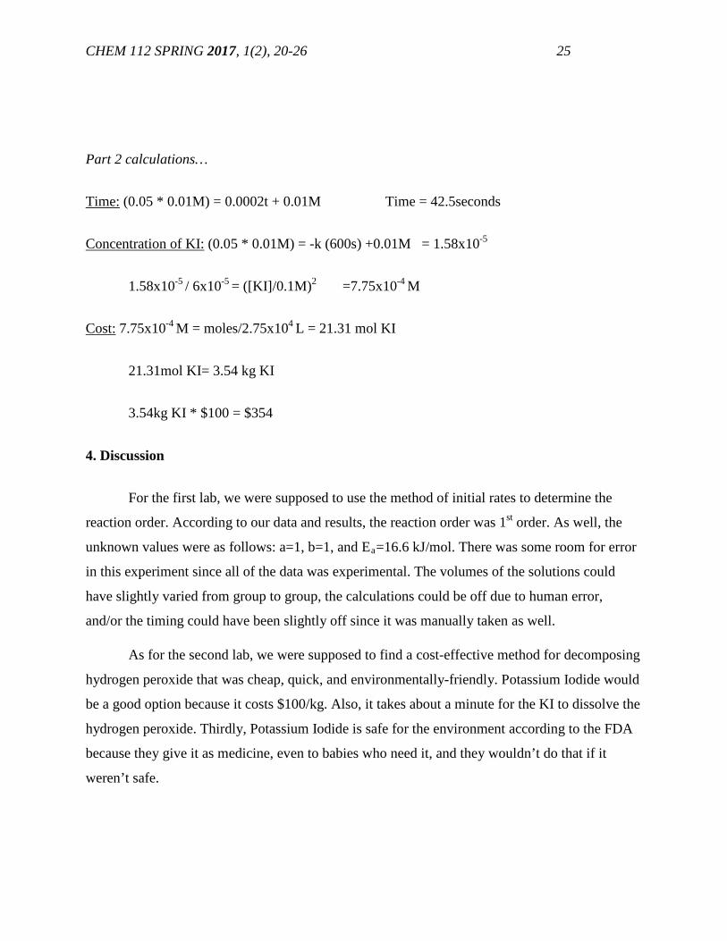
Part 2 calculations…

Time: (0.05 * 0.01M) = 0.0002t + 0.01M Time = 42.5seconds

Concentration of KI: (0.05 * 0.01M) = -k (600s) +0.01M = 1.58x10-5

1.58x10-5 / 6x10-5 = ([KI]/0.1M)2 =7.75x10-4 M

Cost: 7.75x10-4 M = moles/2.75x104 L = 21.31 mol KI

21.31mol KI= 3.54 kg KI

3.54kg KI * $100 = $354

4. Discussion

For the first lab, we were supposed to use the method of initial rates to determine the

reaction order. According to our data and results, the reaction order was 1st order. As well, the

unknown values were as follows: a=1, b=1, and Ea=16.6 kJ/mol. There was some room for error

in this experiment since all of the data was experimental. The volumes of the solutions could

have slightly varied from group to group, the calculations could be off due to human error,

and/or the timing could have been slightly off since it was manually taken as well.

As for the second lab, we were supposed to find a cost-effective method for decomposing

hydrogen peroxide that was cheap, quick, and environmentally-friendly. Potassium Iodide would

be a good option because it costs $100/kg. Also, it takes about a minute for the KI to dissolve the

hydrogen peroxide. Thirdly, Potassium Iodide is safe for the environment according to the FDA

because they give it as medicine, even to babies who need it, and they wouldn’t do that if it

weren’t safe.

CHEM 112 SPRING 2017, 1(2), 20-26 26

References:

https://www.youtube.com/watch?v=3cFhhwM-zdc

https://www.fda.gov/Drugs/EmergencyPreparedness/BioterrorismandDrugPreparedness/ucm072

265.htm

https://www.youtube.com/watch?v=3cFhhwM-zdc

https://www.fda.gov/Drugs/EmergencyPreparedness/BioterrorismandDrugPreparedness/ucm072265.htm

https://www.fda.gov/Drugs/EmergencyPreparedness/BioterrorismandDrugPreparedness/ucm072265.htm

CHEM 112 SPRING 2017, 1(2), 27-32




Equilibrium experiment group: LeChatelier’s Principle and Determination of Kc – Ka of a chemical indicator

Mariana Valenzuela




Abstract: This lab is divided in 2 experiments, the purpose of the first one is to study the effect of changing reactant concentration and temperature on equilibrium, and calculate an equilibrium constant using spectrophotometry. The ultimate goal of the second part of the experiment, is to study the effect of changing acidity on the color of an indicator, create standardized solutions of indicator in buffers of different acidity and finally, determine the equilibrium constant of a chemical indicator.


In chemistry, Le Chatelier's principle or "The Equilibrium Law", can be used to predict the effect of a change in conditions on a chemical equilibrium. The principle is named after Henry Louis Le Chatelier and sometimes Karl Ferdinand Braun who discovered it independently. It can be stated as:

When any system at equilibrium is subjected to change in concentration, temperature, volume, or pressure, then the system readjusts itself to (partially) counteract the effect of the applied change and a new equilibrium is established.

In other words, whenever a system in equilibrium is disturbed the system will adjust itself in such a way that the effect of the change will be nullified.

OPEN ACCESS

CHEM 112 SPRING 2017, 1(2), 27-32 28

Any change in status quo prompts an opposing reaction in the responding system.

In chemistry, the principle is used to manipulate the outcomes of reversible reactions, often to increase the yield of reactions. In pharmacology, the binding of ligands to the receptor may shift the equilibrium according to Le Chatelier's principle, thereby explaining the diverse phenomena of receptor activation and desensitization. In economics, the principle has been generalized to help explain the price equilibrium of efficient economic systems. In simultaneous equilibrium systems, phenomena that are in apparent contradiction to Le Chatelier's principle can occur; these can be resolved by the theory of response reactions.

Effect of change in concentration

Changing the concentration of a chemical will shift the equilibrium to the side that would reduce that change in concentration. The chemical system will attempt to partially oppose the change affected to the original state of equilibrium. In turn, the rate of reaction, extent, and yield of products will be altered corresponding to the impact on the system.

Effect of change in temperature

The effect of changing the temperature in the equilibrium can be made clear by 1) incorporating heat as either a reactant or a product, and 2) assuming that an increase in temperature increases the heat content of a system. When the reaction is exothermic (ΔH is negative, puts energy out), heat is included as a product, and, when the reaction is endothermic (ΔH is positive, takes energy in), heat is included as a reactant. Hence, whether increasing or decreasing the temperature would favor the forward or the reverse reaction can be determined by applying the same principle as with concentration changes.

Effect of change in pressure

The equilibrium concentrations of the products and reactants do not directly depend on the total pressure of the system but they do depend on the partial pressures of the products and reactants.

Changing total pressure by adding an inert gas at constant volume does not affect the equilibrium concentrations.

Changing total pressure by changing the volume of the system changes the partial pressures of the products and reactants and can affect the equilibrium concentrations.

Effect of change in volume

Changing the volume of the system changes the partial pressures of the products and reactants and can affect the equilibrium concentrations. With a pressure increase due to a decrease in volume, the side of the equilibrium with fewer moles is more favorable and with a pressure decrease due to an increase in volume,

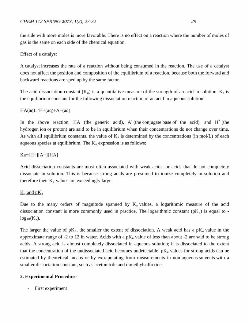
CHEM 112 SPRING 2017, 1(2), 27-32 29

the side with more moles is more favorable. There is no effect on a reaction where the number of moles of gas is the same on each side of the chemical equation.

Effect of a catalyst

A catalyst increases the rate of a reaction without being consumed in the reaction. The use of a catalyst does not affect the position and composition of the equilibrium of a reaction, because both the forward and backward reactions are sped up by the same factor.

The acid dissociation constant (Ka) is a quantitative measure of the strength of an acid in solution. Ka is the equilibrium constant for the following dissociation reaction of an acid in aqueous solution:

HA(aq)⇌H+(aq)+A−(aq)

In the above reaction, HA (the generic acid), A- (the conjugate base of the acid), and H+ (the hydrogen ion or proton) are said to be in equilibrium when their concentrations do not change over time. As with all equilibrium constants, the value of Ka is determined by the concentrations (in mol/L) of each aqueous species at equilibrium. The Ka expression is as follows:

Ka=[H+][A−][HA]

Acid dissociation constants are most often associated with weak acids, or acids that do not completely dissociate in solution. This is because strong acids are presumed to ionize completely in solution and therefore their Ka values are exceedingly large.

Ka and pKa

Due to the many orders of magnitude spanned by Ka values, a logarithmic measure of the acid dissociation constant is more commonly used in practice. The logarithmic constant (pKa) is equal to -log10(Ka).

The larger the value of pKa, the smaller the extent of dissociation. A weak acid has a pKa value in the approximate range of -2 to 12 in water. Acids with a pKa value of less than about -2 are said to be strong acids. A strong acid is almost completely dissociated in aqueous solution; it is dissociated to the extent that the concentration of the undissociated acid becomes undetectable. pKa values for strong acids can be estimated by theoretical means or by extrapolating from measurements in non-aqueous solvents with a smaller dissociation constant, such as acetonitrile and dimethylsulfoxide.


- First experiment

CHEM 112 SPRING 2017, 1(2), 27-32 30

For the first part, we prepared a solution of 25 mL 2.00x10-3 M Fe3+ and 25mL of 2.00x10-3 M SCN- in equal concentrations. Then, we made 5 more solutions, by mixing 5 mL of that previous solution in 5 different ways, each time adding a different disturbance for the reaction. For the first tube we added 2 more drops of the 0.200 M Fe3+ solution. For the second tube we added two drops of the 0.200 M SCN- solution. The third sample was heated and the fourth was cooled while the fifth was not altered and used as a reference tube. Afterwards, we observed and recorded the physical changes of the samples.

For the second part of the experiment we prepared 6 more solutions. Except for our standard sample (9mL), all of them had the same volume of Fe 3+ (5mL) but different concentrations of SCN and water. After mixing them, we recorder the absorbance for each of the samples with the use of a spectrophotometer, and calculated the initial concentrations of the reactants and their equilibrium concentrations.

- Second experiment

For the first part of this experiment we obtained a 50 mL sample of a 4.42 pH standard buffer. Afterwards we took two samples of 0.10M HCl and 0.10M NaOH to create solutions from pH 3 to pH 11. Then, we placed 20 drops of these solutions with different pH values plus two drops of indicator (green) per sample in a 24-well plastic well plate, and we recorded the observations.


- Experiment #1

Tube # Fe 3+ (mL) 2.00x10-3 M SCN (mL)

Water (mL) Absorbance

Std 9.0 of 0.2 M 1 0 0.114

1 5.0 of 0.002M 1 4 0.188

2 5.0 of 0.002M 2 3 0.360

3 5.0 of 0.002M 3 2 0.442

4 5.0 of 0.002M 4 1 0.530

CHEM 112 SPRING 2017, 1(2), 27-32 31

5 5.0 of 0.002M 5 0 0.697

Table 1. Effect of different concentrations of SNC and water on a FeSCN 2+ solution on its absorbance value.

The observations followed the results:

1. The tube with more concentration of Fe presented more intensity in its red color.

2. The tube with more concentration of SCN looked redder.

3. Increasing the temperature for tube #3 resulted in a much lighter yellow color.

4. Cooling test tube #4 made it to be slightly red, basically orange.

- Experiment#2

Our three first samples maintained a yellow color, but the fourth one changed its color to light green. The fifth one had a much darker green color. The sixth sample turned light blue, the seventh solution had a darker blue, and the eight one had an indigo color. Sample #9 had a much darker blue color, almost black.

After having these results we determined that the pH range over which our indicator completed its color change was 5 to 8, and we picked pH values of 5.5, 6.0, 6.5, 7.0 and 7.5 to prepare 5 more solutions that followed this pH values. Moreover, we filled a 6th tube with pH 12. Afterwards we evaluated the analytical wavelength of the pH 12 solution in order to calculate the absorbance of the other 5 samples at this peak.

tube # pH [H+] abs abs/abs ref Hln fraction Ka pKa

1 5,5 3,16228E-06 0,054 0,030033 0,969967 9,79146E-08 7,009153

2 6,01 9,77237E-07 0,147 0,081758 0,918242 8,70102E-08 7,06043

3 6,51 3,0903E-07 0,337 0,18743 0,81257 7,1282E-08 7,14702

CHEM 112 SPRING 2017, 1(2), 27-32 32

4 7,02 9,54993E-08 0,947 0,526696 0,473304 1,06272E-07 6,97358

5 7,52 3,01995E-08 1,169 0,650167 0,349833 5,6126E-08 7,250836

Table 3. Effect of different pH values on the Ka (acidity constant) and pKa (the negative base 10 logarithm of the acid dissociation constant).

The average value for the pKa was 7,088204 with a standard deviation of 0.1187.


For both experiments we were able to observe the LeChatelier’s Principle in action, as we disturbed in different ways the concentration of the solutions and they shifted either to the products or reactants side depending on their concentrations after the disturbances. From the first experiment, we can conclude that it does not matter which one of the reactants or products is added, the reaction will shift in order to complete equilibrium. Moreover we could see that a red color in the indicator was telling us that the reaction was shifting away from the reactants, as we added more of both for test tube #1 and #2. From test tubes #3 and #4 we conclude that the temperature also has an effect on equilibrium. We concluded that the reaction was exothermic, because when we added heat, the solution turned lighter, and when we removed heat, the solution became orange. From the second experiment we concluded that indicators are also good to measure pH, and indicate how acid or basic a solution is.

Acknowledgments

The author gratefully acknowledges his lab partner Austin R. Johnson for his assistance in performing the experiment and all other aspects of the process, including data collection, statistical calculations, and lab clean-up to enumerate a few.


CHEM 112 SPRING 2017 1(2), 33-36




Equilibrium #1 and Equilibrium #2

Chloe Frye



Received: May 6, 2016 / Accepted: May 13, 2017 / Published: May 22, 2017 Abstract: The purpose of the experiments, Equilibrium 1 and Equilibrium 2, was to study chemical equilibrium. We looked at how chemical reactions can be shifted backwards and forwards. Spectrophotometry was used in both experiments to measure absorbance and wavelengths. More specifically, for Equilibrium 1, LaChatelier’s principle was used to determine Kc, and spectrophotometry was used to get the necessary information to calculate the equilibrium constant. For Equilibrium 2, we also used spectrophotometry to calculate the equilibrium constant, but we did this by creating solutions with different pH levels and color changes using indicator.

1. Introduction

Chemical equilibrium is when in a reaction, the reactants and products coexist no matter how long the reaction sits there. When a chemical reaction is shifted backwards, more reactants are created, and when a chemical reaction is shifted forward, more products are created. LaChatelier’s principle also acknowledges how change in temperature affects reactions. For example, if a reaction is endothermic, heat will be a reactant, and if the reaction is exothermic, heat will be a considered a product. In general, to find the equilibrium constant, k, the formula K=[products]/[reactants] will be used.

2. Materials and Methods

In the experiment Equilibrium 1, the following materials were used: .200 M Fe3+, .200 M SCN-, volumetric flasks for dilution, pipets, graduated cylinders, test tubes, an ice bath, a hot plate, and the spectrophotometer/LoggerPro.

OPEN ACCESS

CHEM 112 SPRING 2017, 1(2), 33-36 34

Part 1 of the experiment: After obtaining the needed materials, 2 diluted solutions were made by pipetting 1 mL of each solution into separate volumetric flasks and adding water to the etched line. Part 2 of the experiment: Using 5 test tubes labeled 1-5, we added 5 mL of the part 1 solutions to each one. Two drops of the undiluted .2 M Fe3+ was added to tube 1, two drops of the undiluted .2 M SCN- was added to tube #2, tube #3 was heated using a boiling water bath, and tube #4 was cooled using an ice bath. The resulting colors of each tube were then compared to each other and tube #5. Part 3 of the experiment: Now 6 test tubes are used; in the standard tube, 9 mL of .2 M Fe3+ and 1 mL of 0.002 M SCN- was added and mixed. In tubes 1-5, 5 mL of 0.002 M Fe3+ and (from tubes 1-5), 1 mL to 5 mL 0.002 M SCN- were added and mixed in. Using a spectrophotometer, we measured the absorbance of the six solutions. Finally, using an excel spreadsheet, we used these values to calculate K. In the experiment Equilibrium 2, the materials needed were: standard buffer, .10 M HCl, .10 M NaOH, beakers, droppers, and the pH probe/LoggerPro. Part 1 of the experiment: First, using the standard buffer, HCl, and NaOH, we created solutions with pH ranging from 3-12 and put each into a well plate. Next, we added indicator to each well to observe the color change finding that the color change happened from pH 3-5. Part 2: From part 1, we determined that the pH values we needed to use were 3.0, 3.5, 4.0, 4.5, 5, and 12. Using NaOH and HCl again we created solutions with each of these pH values and added 5 mL of each to separate test tubes. Part 3: We used spectrophotometry and found the analytical wavelength by finding the highest abs value of the 12 pH solution. Using this analytical wavelength, we found the absorbance values for test tubes 1-5.

3. Results

Equilibrium 1 Part 1 Observations

Tube # Observation 1 Darker orange than #5 2 Red orange, darker than #5 3 Clear, light orange 4 A tiny bit darker than tube #5, lighter than tube

#1 5 Normal orange Results table from excel: tube # absorbance diluted

[fe3+]0 diluted [SCN-]0

[FeSCN2+]eq [Fe3+]eq [SCN-]eq Kc

1 0.096 0.001 0.0002 0.000025 0.000975 0.000175 146.520

CHEM 112 SPRING 2017, 1(2), 33-36 35

2 0.352 0.001 0.0004 0.000093 0.000907 0.000307 333.993 3 0.421 0.001 0.0006 0.00011 0.00089 0.00049 252.236 4 0.55 0.001 0.0008 0.00015 0.00085 0.00065 271.493 5 0.695 0.001 0.001 0.00018 0.00082 0.00082 267.698 Standard solution (9mL .2 M Fe3+, 1 mL .002 M SCN-) absorbance: .754 Avg Kc: 254.4 Standard deviation: 67.9 Equilibrium 2 Analytical wavelength used to find abs: 618.5 Results from excel: tube # pH [H+] Abs Abs/Absref Hln fraction Ka pKa 1 3 0.001 0.042 0.0227027 0.9772973 2.32301E-

05 4.633949

2 3.5 0.000316228 0.084 0.04540541 0.95459459 1.50414E-05

4.822711

3 4 0.0001 0.265 0.14324324 0.85675676 1.67192E-05

4.776783

4 4.5 3.16228E-05 0.666 0.36 0.64 1.77878E-05

4.749877

5 5 0.00001 1.091 0.58972973 0.41027027 1.43742E-05

4.842417

6 12 1E-12 1.85 Average pKa: 4.8 Standard deviation: 0.08


For Equilibrium 1, based on the results, the standard solution had an absorbance of 0.754. For tubes # 1-5, the absorbance increased based on the amount of SCN- added. Since tube #5 had 4 more mL of SCN-, the absorbance was significantly higher. These absorbance values were used to calculate the different K values, and the average value was 254.4 with a standard deviation of 67.9. For equilibrium 2, the analytical wavelength used to find the absorbance values was 618.5, and was found from the solution with a pH of 12, which ended up having an absorbance value of 1.85. The results from the calculations show that the average pKa is 4.8 with a standard deviation of 0.08. Looking at a pKa table, we can determine that the solution is a carboxylic acid and is strongly acidic. This makes sense and relates to post lab question 2 because the indicator showed a color change in the solutions with low pH values under 7, which means that there is a strong acid.

CHEM 112 SPRING 2017, 1(2), 33-36 36

Acknowledgments

The author gratefully acknowledges her lab partner Eli Giddens for his assistance in the experiments Equilibrium #1 and Equilibrium #2, which are located in the Spring 2017 Chemistry 112 Lab Manual.

CHEM 112 SPRING 2017, 1(2), 37-44




Dissociation of Acetic Acid and Acetate and the Molecular Structure and Acid Strength

Logan Felton

Department of Chemistry, Indiana University of Pennsylvania, Indiana, PA 15705


Received: May 6, 2017 / Accepted: May 13, 2017 / Published: May 22, 2017 Abstract: This chemistry report presents the data and results from the acid-base experiments that were performed in our chemistry 112 lab. The data and results are based on successful strategies using the Brønsted-Lowry definition of acids and bases and lewis structures. The purpose of these experiments is to investigate the difference between strong and weak acids, calculate the relationship between pH and [H3O+], calculate acid-base properties of an anion, use molecular orbital calculations to determine properties of weak organic acids, plot potential correlations between calculated properties and Ka, analyze data to determine physical bases between molecular structure and Ka.


In these acid-base experiments, the Brønsted-Lowry definition of acid and bases was used. The Brønsted-Lowry definition states that acids are defined as proton donors, and bases are defined as proton acceptors. We used this in order to investigate the difference between strong and weak acids, calculate the relationship between pH and [H3O+], and calculate acid-base properties of an anion. We also determined properties of weak organic acids and compared it to the Ka. This is important because the concept of acid and bases is one of the most powerful in chemistry and is very relevant to everyday life because all of the chemical changes in the human body occur in an aqueous environment.

OPEN ACCESS

CHEM 112 SPRING 2017, 1(2), 37-44 38

2. Experimental Procedure for Creation of Hot Pack

To collect data from the first experiment, Acid-Base #1: Acetic Acid and Acetate, we made three different concentrations of each acid using a dilution process. The concentrations of the acidic solutions were 1.0 M, 0.1 M, and 0.01 M. We then measured the pH of each solution and recorded the data. To collect data from the second experiment, Acid-Base #2: Molecular structure and Acid strength, we used computational methods, WebMO. We built the acids using lewis structures to analyze and record C-O bond distances, O-H bond distances, atomic charge on the acidic hydrogen and charge on the acidic oxygen atom. The data was assessed in order to determine if there was a positive, negative, or no correlation.


I. Acid-Base #1: Acetic Acid and Acetate Table 1. [HCl]0 pH [H+] % dissociation

1.0 -0.24 1.737800829 173.7800829

0.1 0.55 0.281838293 281.8382931

0.01 1.44 0.036307805 363.0780548

Table 2. [HAc]0 pH [H+]eq [Ac

-]eq [HAc]eq Ka % dissociation

pKa

1.0 2.0 0.01 0.01 0.99 0.00010101 1 3.995635195

0.1 2.55 0.002818383 0.002818383 0.097181617 8.17365E-05

2.818382931 4.087584121

0.01 3.05 0.000891251 0.000891251 0.009108749 8.7205E-05 8.912509381 4.059458738

CHEM 112 SPRING 2017, 1(2), 37-44 39

Table 3. [Ac]0 pH pOH [OH-]eq [HAc]eq [Ac

-]eq Kb pKb

0.1 7.84 6.16 6.91831E-07 6.91831E-07 0.099999308 4.78633E-12 11.319997

0.01 7.67 6.33 4.67735E-07 4.67735E-07 0.009999532 2.18786E-11 10.65997969

II. Acid-Base #2: Molecular Structure and Acid Strength Table 4. Neutral Acids pKa O-H bond

distance Å C-O bond distance Å

Charge on Acidic H

Charge on Acidic O

CH3COOH 4.76 0.952 1.355 0.227 -0.311

CH2ClOOH 2.86 0.952 1.356 0.231 -0.308

CHCl2COOH 1.35 0.952 1.353 0.234 -0.294

CCl3COOH 0.56 0.952 1.351 0.236 -0.281

CH2FCOOH 2.59 0.952 1.354 0.232 -0.305

NO2CH2COOH 1.68 0.952 1.358 0.237 -0.31

CHF2COOH 1.34 0.952 1.343 0.211 -0.239

CHEM 112 SPRING 2017, 1(2), 37-44 40

Figure 1. Pka vs. O-H bond distance

Figure 2. pKa vs. C-O bond

CHEM 112 SPRING 2017, 1(2), 37-44 41

Figure 3. pKa vs charge on acidic H

Figure 4. pKa vs. charge on acidic O

CHEM 112 SPRING 2017, 1(2), 37-44 42

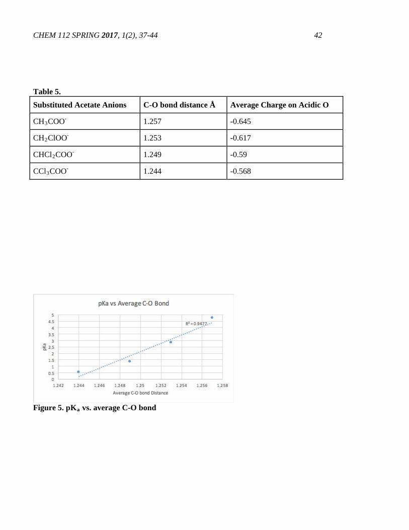
Table 5. Substituted Acetate Anions C-O bond distance Å Average Charge on Acidic O

CH3COO- 1.257 -0.645

CH2ClOO- 1.253 -0.617

CHCl2COO- 1.249 -0.59

CCl3COO- 1.244 -0.568

Figure 5. pKa vs. average C-O bond

CHEM 112 SPRING 2017, 1(2), 37-44 43

Figure 6. pKa vs. average charge on Acidic O


In Acid-Base #1, we studied the difference between strong and weak acids, calculated the relationship between pH and [H3O+], and calculated acid-base properties of an anion. We found that the percent dissociation for HCl increased as the concentration of the acid decreased. 0.01 M of HCl had the highest % dissociation of 363.08 %. The pH and percent dissociation of the HCl solution differs than those of the acetic acid solution of similar concentrations because HCl is a stronger acid than the acetic acid. The reasoning behind this is because HCl is a stronger acid and it completely dissociates in water. It has more of a tendency to lose a proton versus the acetic acid. A stronger acid has a lower pH than a weaker acid regardless of the concentration. In calculations with weak acid, it is usually assumed that the initial concentration is essentially unchanged by dissociation. Based on our data, this statement seems to be a valid assumption for acetic acid. Based on our results in table 2, the initial concentration is 1.0 M and the concentration at equilibrium is 0.99 or approximately 1.0 M. The initial concentration after dilution is 0.1 M and the concentration at equilibrium is 0.097 or approximately 0.1M. The initial concentration after dilution again is 0.01 M and the concentration at equilibrium is 0.009 or approximately 0.001 M. The corresponding assumption seems to also apply to weak bases. For example, our data for sodium acetate has an initial concentration of 0.1M and at equilibrium is 0.09M or approximately 0.1M. After dilution, the initial concentration is 0.01 and the assumption still applies with an equilibrium concentration at 0.0099 M or approximately 0.01 M. The percent error for our acetic acid was -14.61%. The percent error for our sodium acetate was 18.81%. For Acid-Base #2, we used molecular orbital calculations to determine properties of weak organic acids. We found that hypothesis 1, as acidity increased, there was a weakening of the O-H bond to the acidic H, to not be supported by our data. The poor R squared values failed to support the hypothesis. The r squared value in figure 1, pka vs O-H bond, had a value of 0. The r squared value in figure 2, pka vs. C-0 bond, had a value of 0.16964. Both plots showed a weak correlation coefficient. We found that hypothesis 2, as acidity increased, it stabilized the anion by reducing terminal O’s negative charge, to be supported by the data we collected. In figure 5, pKa vs. average C-O bond, there was a positive strong correlation coefficient with an r squared value of 0.9477. In figure 6, pKa vs

CHEM 112 SPRING 2017, 1(2), 37-44 44

average charge on acidic O, there was a strong correlation coefficient with an r squared value of 0.9851. We found hypothesis 3, as acidity increased, there was a change in charge distribution on the neutral acid, to not be supported with the data configured. In figure 3, pKa vs. charge on acidic H, there was a weak correlation coefficient with an r squared value 0.00853. In figure 4, pKa vs. charge on acidic O, there was a weak correlation with an r squared value of 0.57562. It was found that as the number of terminal chlorine atoms increased, the pKa decreased. For example, for CH2ClOOH, the pKa was 2.86 with only one chlorine atom. For CHCl2COOH, the pKa decreased to 1.35 with two chlorine atoms. For CCl3COOH, the pKa decreased to 0.56 with three chlorine atoms. This also helps to support hypothesis 2 that as acidity increases, it stabilizes the anion by reducing terminal O’s negative charge.

Acknowledgments

The author gratefully acknowledges her lab partner Anna Deabenderfer for her assistance in performing the experiment and all other aspects of the process, including data collection, statistical calculations, and lab clean-up to enumerate a few. The author also gratefully acknowledges her laboratory instructor, Dr. H. Tang for helping to further and enhance her knowledge in the field of chemistry.


Chemistry Department

975 Oakland Avenue

143 Weyandt Hall


Indiana, PA 15705

www.iup.edu/chemistry

Documents

CHEM 112 A04&09 GENERAL CHEMISTRY II … · the structures of different organic molecules and obtain ... For the aprotic liquids, ... determination of evaporation rate as the independent