CHEE825/435 - Fall 2005J. McLellan1 Dynamic Experiments Maximizing the Information Content for Control Applications

CHEE825/435 - Fall 2005

J. McLellan 1

Dynamic Experiments

Maximizing the Information Content for Control Applications

CHEE825/435 - Fall 2005

J. McLellan 2

Outline

• types of input signals• characteristics of input signals• pseudo-random binary sequence (PRBS) inputs• other input signals• inputs for multivariable identification• input signals for closed-loop identification

CHEE825/435 - Fall 2005

J. McLellan 3

Types of Input Signals

• deterministic signals» steps» pulses» sinusoids

• stochastic signals» white noise» correlated noise

• what are the important characteristics?

CHEE825/435 - Fall 2005

J. McLellan 4

Outline

• types of input signals• characteristics of input signals• pseudo-random binary sequence (PRBS) inputs• other input signals• inputs for multivariable identification• input signals for closed-loop identification

CHEE825/435 - Fall 2005

J. McLellan 5

Important Characteristics

• signal-to-noise ratio• duration• frequency content• optimum input (deterministic / random) depends on

intended end-use– control– prediction

CHEE825/435 - Fall 2005

J. McLellan 6

Signal-to-Noise Ratio

• improves precision of model» parameters» predictions

• avoid modeling noise vs. process• trade-off

» short-term pain vs. long-term gain» process disruption vs.expensive retesting / poor

controller performance

• note - excessively large inputs can take process into region of nonlinear behaviour

CHEE825/435 - Fall 2005

J. McLellan 7

Example - Estimating 1st Order Process Model with RBS Input

True model y tq

qu t a t( )

.

.( ) ( )

10 6

1 0 75

1

1

0 5 10 15 20 25 30 35 400

0.5

1

1.5

2

2.5

3

3.5

4

Time

Step Response

confidenceintervals aretighter with increasing SNR

1:1

10:1

less preciseestimate ofsteady stategain

more preciseestimateof transient

CHEE825/435 - Fall 2005

J. McLellan 8

Example - Estimating First-Order Model with Step Input

0 5 10 15 20 25 30 35 40-2

-1

0

1

2

3

4

5

6

Time

Step Response

1:1

10:1

more preciseestimate ofgain vs.RBS input

less precise estimateof transient

response99% confidenceinterval

CHEE825/435 - Fall 2005

J. McLellan 9

Test Duration

• how much data should we collect?• want to capture complete process dynamic response• duration should be at least as long as the settling

time for the process (time to 95% of step change)• failure to allow sufficient time can lead to misleading

estimates of process gain, poor precision

CHEE825/435 - Fall 2005

J. McLellan 10

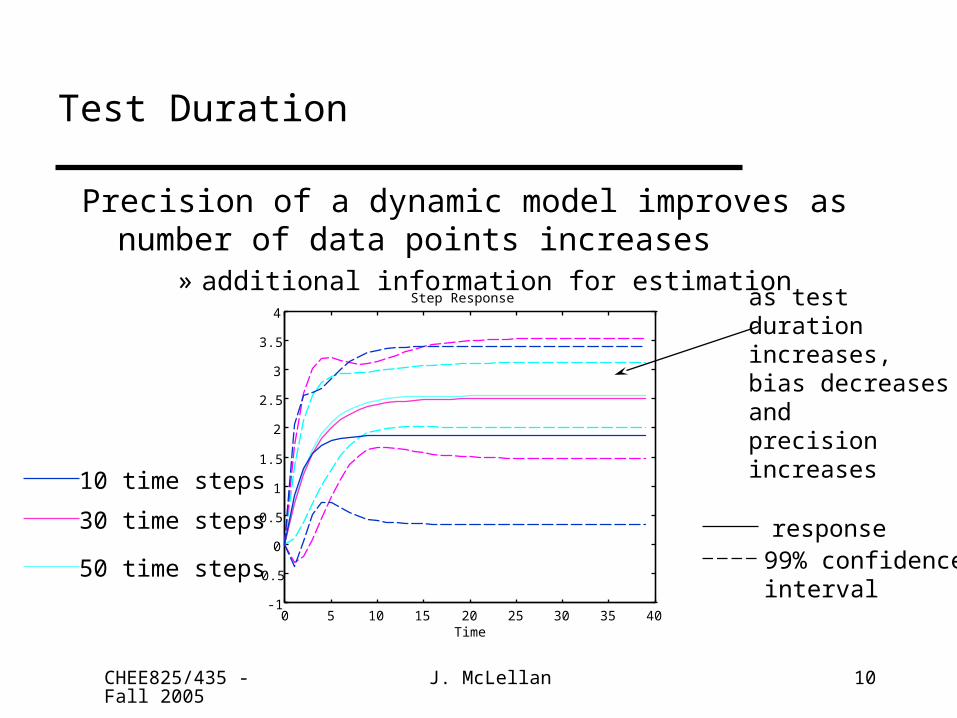
Test Duration

Precision of a dynamic model improves as number of data points increases

» additional information for estimation

0 5 10 15 20 25 30 35 40-1

-0.5

0

0.5

1

1.5

2

2.5

3

3.5

4

Time

Step Response as test duration increases,bias decreasesand precision increases


10 time steps

30 time steps

50 time steps

CHEE825/435 - Fall 2005

J. McLellan 11

“Dynamic Content”

• what types of transients should be present in input signal?– excite process over range of interest– model is to be used in controller for:

» setpoint tracking» disturbance rejection

• need orderly way to assess dynamic content» high frequency components - fast dynamics» low frequency components - slow dynamics / steady-

state gain

CHEE825/435 - Fall 2005

J. McLellan 12

Frequency Content - Guiding Principle

The input signal should have a frequency content matching

that for end-use.

CHEE825/435 - Fall 2005

J. McLellan 13

Looking at Frequency Content

• ideal - match dynamic behaviour of true process as closely as possible

• goal - match the frequency behaviour of the true process as closely as possible

• practical goal - match frequency behaviour of the true process as closely as possible, where it is most important

CHEE825/435 - Fall 2005

J. McLellan 14

Experimental Design Objective

Design input sequence to minimize the following:

design

cost

error in

predicted frequency response

importance

function

our designobjectives

difference in predicted vs.true behaviour- function of frequency, andthe input signal used

CHEE825/435 - Fall 2005

J. McLellan 15

Accounting for Model Error - Interpretation

Optimal solution in terms of frequency content:

spectral density

frequencyerror in model vs.true process

spectral density

frequency

importance to ourapplication

low

highvery important

not important*J=

CHEE825/435 - Fall 2005

J. McLellan 16

Accounting for Model Error

Consider frequency content matching

Goal - best model for final application is obtained by minimizing J

J G e G e C j dj T j T

frequencyrange

$( ) ( ) ( ) 2}

bias in frequencycontent modeling

}

importanceof matching- weightingfunction

CHEE825/435 - Fall 2005

J. McLellan 17

Example - Importance Function for Model Predictive Control

spectral density

frequency

high frequency disturbance rejectionperformed by base-levelcontrollers- > accuracy not importantin this range

require good estimateof steady state gain,slower dynamics

CHEE825/435 - Fall 2005

J. McLellan 18

Desired Input Signal for Model Predictive Control

• sequence with frequency content concentrated in low frequency range– PRBS (or random binary sequence - RBS)

• step input– will provide for good estimate of gain, but not of transient

dynamics

CHEE825/435 - Fall 2005

J. McLellan 19

Control Applications

For best results, input signal should have frequency content in range of closed-loop process bandwidth– recursive requirement!– closed-loop bandwidth will depend in part on controller

tuning, which we will do with identified model

CHEE825/435 - Fall 2005

J. McLellan 20

Control Applications

One Approach:Design input frequency content to include:– frequency band near bandwidth of open-loop plant (~1/time

constant)– frequency band near desired closed-loop bandwidth– lower frequencies to obtain good estimate of steady state

gain

CHEE825/435 - Fall 2005

J. McLellan 21

Frequency Content of Some Standard Test Inputs

frequency

power

low frequency - like a series of long steps

high frequency - like a series of short steps

CHEE825/435 - Fall 2005

J. McLellan 22


Step Input

power

frequency0

power is concentrated at low frequency - provides good information about steady state gain, more limited infoabout higher frequency behaviour

CHEE825/435 - Fall 2005

J. McLellan 23

Example - Estimating First-Order Model with Step Input

0 5 10 15 20 25 30 35 40-2

-1

0

1

2

3

4

5

6

Time

Step Response

1:1

10:1

more preciseestimate ofgain vs.RBS input

less precise estimateof transient


CHEE825/435 - Fall 2005

J. McLellan 24


White Noise – approximated by pseudo-random or random binary

sequences

power

frequency

power is distributed uniformlyover all frequencies- broader information, but poorerinformation about steady state gain

ideal curve

CHEE825/435 - Fall 2005

J. McLellan 25

Example - Estimating 1st Order Process Model with RBS Input

0 5 10 15 20 25 30 35 400

0.5

1

1.5

2

2.5

3

3.5

4

Time

Step Response

less preciseestimate ofsteady stategain

more preciseestimateof transient

1:1

10:1


CHEE825/435 - Fall 2005

J. McLellan 26


Sinusoid at one frequency

power

frequency

power concentrated at onefrequency correspondingto input signal- poor information aboutsteady state gain, otherfrequencies

CHEE825/435 - Fall 2005

J. McLellan 27


Correlated noise– consider u

qucorr white

01

1 0 9 1.

.

power

frequency

variability is concentrated at lowerfrequencies- will lead to improved estimate ofsteady state gain, poorer estimate ofhigher frequency behaviour

CHEE825/435 - Fall 2005

J. McLellan 28

Persistent Excitation

In order to obtain a consistent estimate of the process model, the input should excite all modes of the process

– refers to the ability to uniquely identify all parts of the process model

CHEE825/435 - Fall 2005

J. McLellan 29

Persistent Excitation

Persistent excitation implies a richness in the structure of the input– input shouldn’t be too correlated

Examples– constant step input

» highly correlated signal » provides unique info about process gain

– random binary sequence » low correlation signal» provides unique info about additional model parameters

CHEE825/435 - Fall 2005

J. McLellan 30

Persistent Excitation - Detailed Discussion

• Example - consider an impulse response process representation

• formulate estimation problem in terms of the covariances of u(t)

• can we obtain the impulse weights?• consider estimation matrix • persistently exciting of order n - definition• spectral interpretation

CHEE825/435 - Fall 2005

J. McLellan 31

Persistence of Excitation

• Add in defn in terms of covariance -

CHEE825/435 - Fall 2005

J. McLellan 32

Outline

• types of input signals• characteristics of input signals• pseudo-random binary sequence (PRBS) inputs• other types of input signals• inputs for multivariable identification• input signals for closed-loop identification

CHEE825/435 - Fall 2005

J. McLellan 33

Pseudo-Random Binary Sequences

(PRBS Testing)

CHEE825/435 - Fall 2005

J. McLellan 34

What is a PRBS?

• approximation to white noise input• white noise

» Gaussian noise» uncorrelated» constant variance» zero mean

• PRBS is a means of approximating using two levels (high/low)

CHEE825/435 - Fall 2005

J. McLellan 35

PRBS

• traditionally generated using a set of shift registers• can be generated using random numbers

– switch to high/low values

• generation by finite representation introduces periodicity

» try to get period large relative to data length

CHEE825/435 - Fall 2005

J. McLellan 36

PRBS Signal

Alternates in a random fashion between two values:

0 20 40 60 80 100-2

-1.5

-1

-0.5

0

0.5

1

1.5

2prbs input

time step

value

input magnitude

minimumswitchingtime

test duration

CHEE825/435 - Fall 2005

J. McLellan 37

How well does PRBS approximate white noise?

Compare spectra:

10-2

10-1

100

101

102

10-1

100

101

frequency

power

spectrum for 100 point PRBS signaltheoretical spectrumfor white noise

note concentrationof PRBS signalin lower frequencyrange

1 .minimum switch time

CHEE825/435 - Fall 2005

J. McLellan 38

PRBS Design Parameters

Amplitude– determines signal-to-noise ratio

» precision vs. process upsets– large magnitudes may bring in process nonlinearity as more

of the operating region is covered– could result in poor model because of

» estimation difficulties - e.g., gains, time constants not constant over range

» model selection difficulties - lack of clear indication of process structure

CHEE825/435 - Fall 2005

J. McLellan 39

PRBS Design Parameters

Minimum switch time– shortest interval in which value is held constant– value is sampling period for process– rule of thumb -> ~20-30% of process time constant– influences frequency content of signal

» small -> more high frequency content» large -> more low frequency content

≥

CHEE825/435 - Fall 2005

J. McLellan 40

PRBS Design Procedure

• select amplitude» two levels

• decide on desired frequency content» high/low

• shape frequency content by– adjusting minimum switching time

OR by filtering PRBS with first-order filter

OR by modifying PRBS to make probability of switching 0.5

CHEE825/435 - Fall 2005

J. McLellan 41

Other PRBS Design Parameters - Switching Probability

• another method of adjusting frequency content• given a two-level white noise input e(t), define input to

process as

• as increases, input signal switches less frequently --> lower frequencies are emphasized

u tu t withprobabilit y

e t with probability( )

( )

( )

1

1

CHEE825/435 - Fall 2005

J. McLellan 42

Switching Probability ...

• as increases to 1, starts to approach a step• this approach shapes frequency content by

introducing correlation– same correlation structure can be introduced using first-

order filter

CHEE825/435 - Fall 2005

J. McLellan 43

Manual vs. Automatic PRBS Generation

• PRBS inputs can be generated automatically – using custom software– using Excel, Matlab, MatrixX, Numerical Recipes routine, ...

• shaping frequency content is usually an iterative procedure– select design parameters (e.g., switching time) and assess

results, modify as required– select filter parameters

CHEE825/435 - Fall 2005

J. McLellan 44

Manual Generation

• sequence of step moves determined manually– can resemble PRBS with appropriate design parameters– gain additional benefits beyond single step test

• recommended procedure– decide on a step sequence with desired frequency content

BEFORE experimentation– modify on-line as required, but assess impact of

modifications on input frequency content and thus information content of data set

CHEE825/435 - Fall 2005

J. McLellan 45

A final comment on frequency content...

Increasing low frequency content typically introduces slower steps up/down– brings potential benefit of being able to see initial process

transient– provides an indication of time delay magnitude

CHEE825/435 - Fall 2005

J. McLellan 46

Outline


CHEE825/435 - Fall 2005

J. McLellan 47

What other signals are available & when should they be used?

Sinusoids– particularly for direct estimation of frequency response– introduce combination of sinusoids and reconstruct frequency

spectrum– a sequence of steps of the same duration has same

properties– danger - difficult to “eyeball” delay because no sharp

transients

CHEE825/435 - Fall 2005

J. McLellan 48

What other signals are available, and when should they be used?

Steps and Impulses– represent low frequency inputs– useful for direct transient analysis

» indication of gain, time constants, time delays, type of process (1st/2nd order, over/underdamped)

– step inputs» good estimate of gain» less precise estimate of transients

CHEE825/435 - Fall 2005

J. McLellan 49

Outline


CHEE825/435 - Fall 2005

J. McLellan 50

Dealing with Multivariable Processes

Approaches

• Perturb inputs sequentially and estimate models for each input-output pair (SISO)

• Perturb all inputs simultaneously and estimate models for a given output (MISO)

» using independent input test sequences

» using correlated input test sequences

• Perturb all inputs simultaneously and estimate models for all outputs simultaneously (MIMO)

CHEE825/435 - Fall 2005

J. McLellan 51

SISO Approach

• introduce sequence of independent signals for each input

• estimate SISO transfer functions individually for each input/output pair

• advantage– easier to identify model structure

• disadvantage– reconciling disturbance models for each output– difficult to guarantee all other inputs are constant– residual effects of input test sequences?

CHEE825/435 - Fall 2005

J. McLellan 52

MISO Approach

• introduce independent signals for all inputs, use data for a single output

• estimate transfer functions simultaneously• advantage

– easier to identify model structure

• disadvantage– no information about directionality of process– may not identify most compact representation of process

CHEE825/435 - Fall 2005

J. McLellan 53

Why do we use a MISO approach?

… because of the model form used:

process transfer + disturbance

function model

Approach– estimate transfer functions– fit disturbance to remaining residual error

CHEE825/435 - Fall 2005

J. McLellan 54

Independent Inputs

… are independent when the sequence for one input does not depend on the sequence for another input

CHEE825/435 - Fall 2005

J. McLellan 55

MIMO Approach with Correlated Inputs

• perturb all inputs simultaneously, but with cross-correlated inputs– input 1 has linear association with input 2– chances are when input 1 moves, input 2 also moves

independent inputs correlated inputs

CHEE825/435 - Fall 2005

J. McLellan 56

MIMO Approach with Correlated Inputs

• advantages– indication of process directionality– improved model estimates

• disadvantages– complexity of model– more difficulty recognizing model structure

CHEE825/435 - Fall 2005

J. McLellan 57

Outline


CHEE825/435 - Fall 2005

J. McLellan 58

Input Signals for Closed-Loop Identification

Identification experiments can be conducted with the controllers on automatic.

Scenarios– unstable processes – avoiding disruption of operation

» quality targets» highly integrated processes

CHEE825/435 - Fall 2005

J. McLellan 59

Identification Signals for Closed-Loop Identification

Yt

UtSPt

+-

ControllerGc

ProcessGp

dither signal Wt

X++

CHEE825/435 - Fall 2005

J. McLellan 60

Where should the input signal be introduced?

Options:

Dither at the controller output

– clearer indication of process dynamics– better estimation properties– preferred approach

Perturbations in the setpoint

– additional controller dynamics will be included in estimated model

CHEE825/435 - Fall 2005

J. McLellan 61

What does the closed-loop data represent?

• dither signal case, without disturbances

Open-loop – input-output data represents

Closed-loop– input-output data represents

Y G Wt p t

YG

G GWt

p

p ct

1

CHEE825/435 - Fall 2005

J. McLellan 62

Implications for Input Signal Design

Importance of introducing some external excitation– non-parametric estimation procedures will simply identify

negative inverse of controller– difficult/dangerous to estimate process transfer function from

closed-loop data without external signal

CHEE825/435 - Fall 2005

J. McLellan 63

Implications for Input Signal Design

• can still use RBS, PRBS, and other signals• signal to noise ratio becomes more important

– make dither signal dominate loop– under large dither signal, properties of closed-loop

estimation approach those for open-loop case

• may be necessary to modify frequency content to accommodate closed-loop

CHEE825/435 - Fall 2005

J. McLellan 64

Interesting Point

When the dither signal large, the closed loop experiment is equivalent to filtering dither signal input by

and estimating process transfer function– could be optimal for disturbance rejection controllers

• the input to the process, U(t), is

1

1 G Gp c

)(1

1)( tW

GGtU

cp+=

Documents

CHEE825/435 - Fall 2005J. McLellan1 Dynamic Experiments Maximizing the Information Content for Control Applications