TUE opleiding Werktuigbouwkunde

Chatter detection

in high-speed milling

F.B.J.W.M. Hendriks

Reportnr. DCT 2005.62

Bachelor Eindproject Dynamics and Control Coaches: Ir. R.P.H. Faassen Dr.ir. N. van de Wouw Prof.dr. H. Nijmeijer Eindhoven, April 2005

2

Summary High-speed milling is used frequently in the manufacturing industry. In order to work with maximum efficiency the material removal rate should be as high as possible while maintaining a good surface quality. The material removal rate is restricted due to chatter. Chatter causes rapid wearing of the cutting tool and the milling machine. It also causes an inferior surface quality and noise. Projects have been started to predict and control chatter. However, to be able to control chatter, first it has to be detected. This report discusses the suitability of several sensors for chatter detection. Dedicated experiments have been performed. Based on these experiments, a sensor is chosen, which is suited best for chatter detection.

3

Table of contents Chapter page 1. Introduction 4 1.1 Problem formulation 4 1.2 Contents of this report 4 2. The high-speed milling process and chatter 5 3. Experimental setup 8 3.1 Sensors 8 3.2 Setup 8 4. Experimental results 10 4.1 Data processing 10 4.2 Sound measurements 11 4.3 Accelerometer measurements on the spindle housing 14 4.4 Accelerometer measurements on the workpiece 17 4.5 Striking phenomena 19 5. Conclusions and recommendations 24 References 25 Appendix A: PSD’s of the microphone signal at 42000 rpm 26

4

1. Introduction In modern manufacturing industry, sometimes large amounts of material have to be removed. Often milling is used for this purpose. Milling is most efficient when a high material removal rate is attained. The most important parameters that influence the material removal rate are the spindle speed, the feed per tooth and the axial and radial depth-of-cut. In order to have a large material removal rate, high-speed milling machines are widely used. These machines have very high spindle speeds (typically over 10000 rpm). However, at certain combinations of spindle speed and axial depth-of-cut (and other process parameters) chatter can occur. Chatter is a problem. Chatter relates to heavy cutting tool vibrations, which cause an inferior surface quality, noise and rapid wear of the cutting tool and the machine. Projects have been started to predict chatter and to design controllers which automatically detect chatter and correct the process parameters such that chatter is avoided. An example of such a project is the ‘Chatter Control’ project at TNO Science and Industry in cooperation with the mechanical engineering department of the Technical University of Eindhoven and some partners from industry. This project is a part of the PHD project of Ronald Faassen, which is a part of the ‘Chatter Control’ project. Note that before the process parameters can be corrected, chatter should be detected first. Different sensoring methods exist to detect chatter. The acceleration or the displacement of parts of the machine or workpiece can be measured or the sound the machine and the process produce can be recorded.

1.1 Problem formulation The aim of this project is to give an answer to the question whether chatter can be detected online during milling using sensors. To give an answer to this question, dedicated experiments have been performed with 3 different sensors. The acquired data from these experiments is thoroughly analyzed, especially the transition from no chatter to chatter. Based on this analysis, conclusions will be drawn whether chatter can be detected and which sensor is best for chatter detection.

1.2 Contents of this report In section 2, some theoretical background of the milling process and chatter is presented. Then, in section 3.1, some sensors, which will be compared, are chosen. With these sensors, experiments have been performed on a high-speed milling machine. The setup of the experiments will be discussed in section 3.2. The acquired data from the experiments is then processed in section 4.1. In section 4.2 to section 4.4, analyses in the frequency domain of the different signals are used to give an insight in the usability of the different sensors. Then some striking things that were encountered during the experiments and the processing of the results are discussed in section 4.5. Finally in section 5, conclusions and recommendations are presented.

5

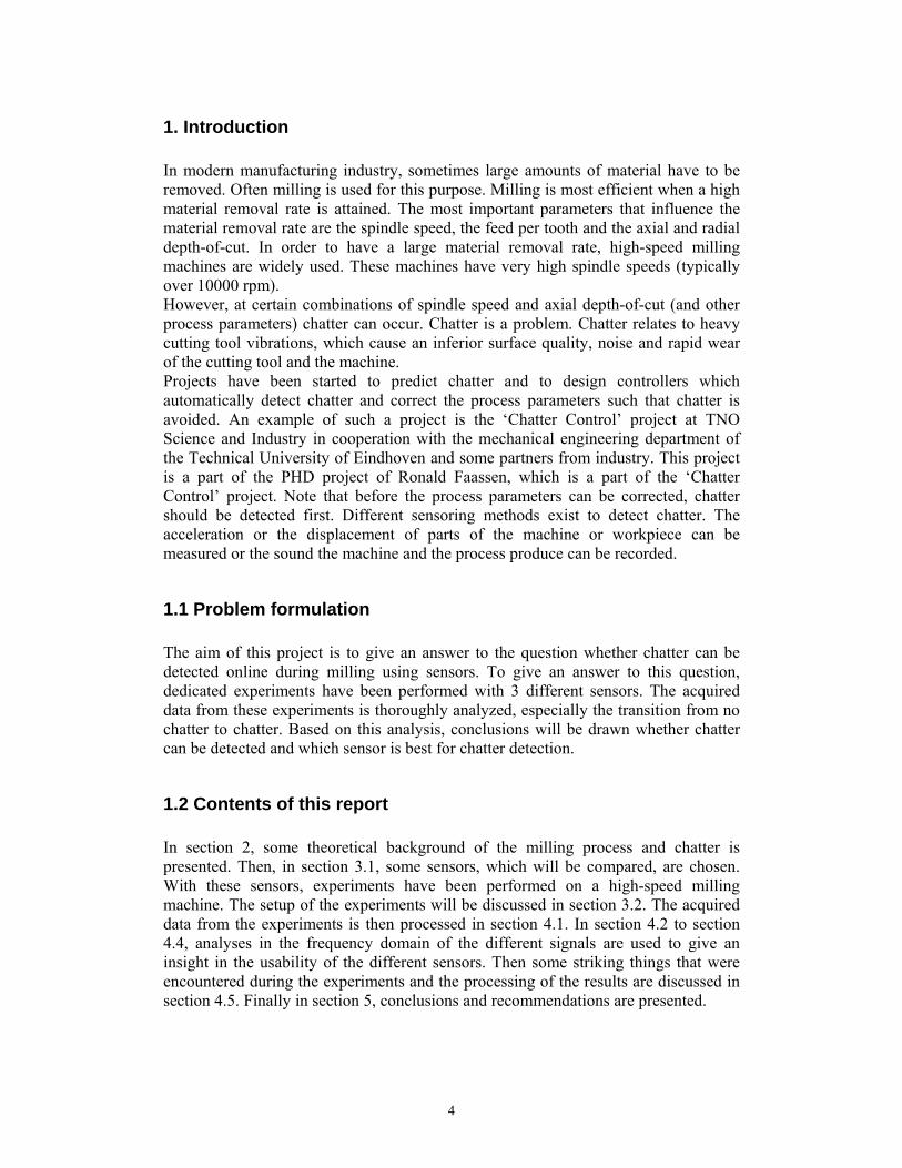
2. The high-speed milling process and chatter In the milling process, material is removed by a rotating cutting tool. The accuracy of the material removal is, among other things, dependent on the static and dynamic properties of the machine and the cutting tool. In order to maintain a high cutting accuracy, the path of the cutting tool should differ as little as possible from the prescribed path. Differences in the actual path and prescribed path of the cutting tool can occur due to chatter. There are different mechanisms that cause chatter. Mode-coupling [9], thermodynamics of the cutting process [3,9], friction between the workpiece and the cutting tool [7,11] and regeneration of waviness of the surface of the workpiece [1] are some causes of chatter. The chatter regarded in this report is due to regeneration of waviness of the surface of the workpiece, i.e. regenerative chatter. Regenerative chatter will be explained in a bit more detail using a simple example. Figure 2.1 shows a schematic representation of the milling process. The cutting tool rotates and moves in positive x-direction. In this way material is removed. The process parameters shown in this figure are the axial depth-of-cut ap, the radial depth-of-cut ae, the spindle speed Ω and the feed per tooth (chip load) fz. The displacement of the tool relative to the prescribed path in x- and y-direction is denoted by ux and uy, respectively. The forces acting on the cutting tool are denoted by Ft and Fr for the tangential force and the radial force, respectively. The rotation angle of the cutting tooth j is denoted by φj.

Figure 2.1 Schematic representation of the milling process [5,6].

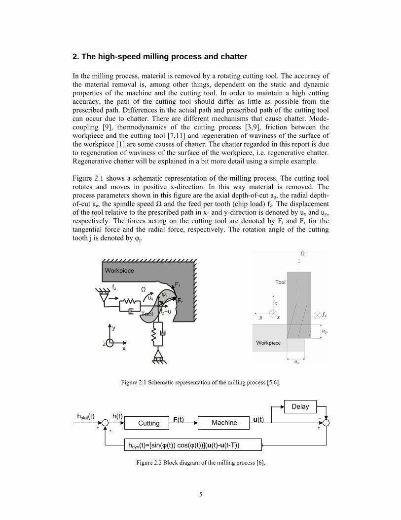
Figure 2.2 Block diagram of the milling process [6].

Ω φj

fz+u

uy

Workpiece

Tool

Ft

Fr

fz

x

y

z

Cutting Machine

Delay

F(t) u(t)

hdyn(t)=[sin(φ(t)) cos(φ(t))](u(t)-u(t-T))

+ +

_

+

hstat(t) h(t)

6

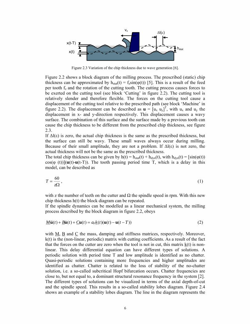
Figure 2.3 Variation of the chip thickness due to wave generation [6].

Figure 2.2 shows a block diagram of the milling process. The prescribed (static) chip thickness can be approximated by hstat(t) = fzsin(φ(t)) [5]. This is a result of the feed per tooth fz and the rotation of the cutting tooth. The cutting process causes forces to be exerted on the cutting tool (see block ‘Cutting’ in figure 2.2). The cutting tool is relatively slender and therefore flexible. The forces on the cutting tool cause a displacement of the cutting tool relative to the prescribed path (see block ‘Machine’ in figure 2.2). The displacement can be described as u = [ux uy]T, with ux and uy the displacement in x- and y-direction respectively. This displacement causes a wavy surface. The combination of this surface and the surface made by a previous tooth can cause the chip thickness to be different from the prescribed chip thickness, see figure 2.3. If ∆l(ε) is zero, the actual chip thickness is the same as the prescribed thickness, but the surface can still be wavy. These small waves always occur during milling. Because of their small amplitude, they are not a problem. If ∆l(ε) is not zero, the actual thickness will not be the same as the prescribed thickness. The total chip thickness can be given by h(t) = hstat(t) + hdyn(t), with hdyn(t) = [sin(φ(t)) cos(φ (t))](u(t)-u(t-T)). The tooth passing period time T, which is a delay in this model, can be described as

Ω=

zT 60 , (1)

with z the number of teeth on the cutter and Ω the spindle speed in rpm. With this new chip thickness h(t) the block diagram can be repeated. If the spindle dynamics can be modelled as a linear mechanical system, the milling process described by the block diagram in figure 2.2, obeys

))()()(()()()( TtttkatCtBtM p −−=++ uuuuu &&& (2) with M, B and C the mass, damping and stiffness matrices, respectively. Moreover, k(t) is the (non-linear, periodic) matrix with cutting coefficients. As a result of the fact that the forces on the cutter are zero when the tool is not in cut, this matrix k(t) is non-linear. This delay differential equation can have different types of solutions. A periodic solution with period time T and low amplitude is identified as no chatter. Quasi-periodic solutions containing more frequencies and higher amplitudes are identified as chatter. Chatter is related to the loss of stability of the no-chatter solution, i.e. a so-called subcritical Hopf bifurcation occurs. Chatter frequencies are close to, but not equal to, a dominant structural resonance frequency in the system [2]. The different types of solutions can be visualized in terms of the axial depth-of-cut and the spindle speed. This results in a so-called stability lobes diagram. Figure 2.4 shows an example of a stability lobes diagram. The line in the diagram represents the

hstat

vc

x(t-T)

x(t)

∆l(ε)

7

chatter boundary. Beneath the line no chatter occurs, whereas above the line chatter occurs. The extra frequencies that occur during chatter are the reason chatter cannot only be detected by looking at the surface quality, but also by listening to the cutting process. Without chatter the sound of the cutting process is calm, only the frequencies from the spindle speed and the tooth cutting can be heard. With chatter the sound is noisy; not one, but a lot of extra frequencies can be heard. This is caused by the non-linearity of this system in the matrix k(t). This will result in a range of chatter frequencies at n*f1±f2, with f1 the tooth passing frequency and f2 the “basic” chatter frequency [8]. So chatter frequencies will occur in pairs around the tooth passing frequency and spindle speed frequency. This fact will be used in order to detect chatter in the next section.

Figure 2.4 Example of a stability lobes diagram.

chatter

no chatter

Spindle speed Ω

Axi

al d

epth

-of-c

ut

8

3. Experimental setup

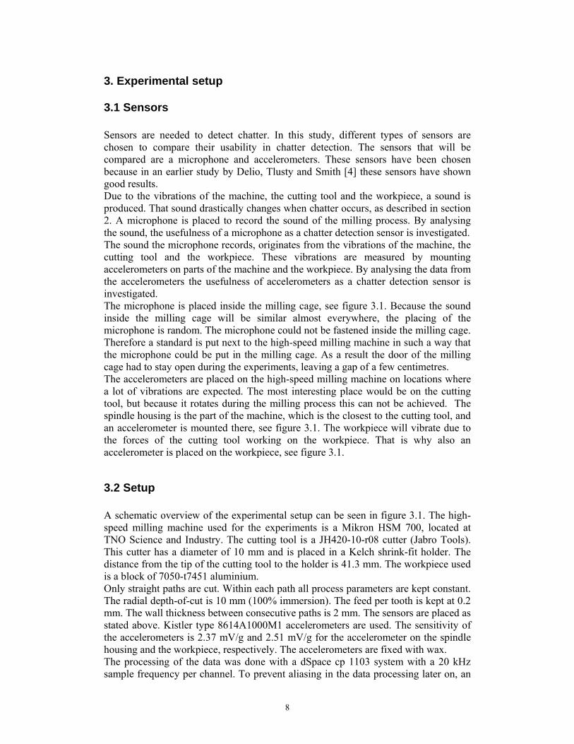
3.1 Sensors Sensors are needed to detect chatter. In this study, different types of sensors are chosen to compare their usability in chatter detection. The sensors that will be compared are a microphone and accelerometers. These sensors have been chosen because in an earlier study by Delio, Tlusty and Smith [4] these sensors have shown good results. Due to the vibrations of the machine, the cutting tool and the workpiece, a sound is produced. That sound drastically changes when chatter occurs, as described in section 2. A microphone is placed to record the sound of the milling process. By analysing the sound, the usefulness of a microphone as a chatter detection sensor is investigated. The sound the microphone records, originates from the vibrations of the machine, the cutting tool and the workpiece. These vibrations are measured by mounting accelerometers on parts of the machine and the workpiece. By analysing the data from the accelerometers the usefulness of accelerometers as a chatter detection sensor is investigated. The microphone is placed inside the milling cage, see figure 3.1. Because the sound inside the milling cage will be similar almost everywhere, the placing of the microphone is random. The microphone could not be fastened inside the milling cage. Therefore a standard is put next to the high-speed milling machine in such a way that the microphone could be put in the milling cage. As a result the door of the milling cage had to stay open during the experiments, leaving a gap of a few centimetres. The accelerometers are placed on the high-speed milling machine on locations where a lot of vibrations are expected. The most interesting place would be on the cutting tool, but because it rotates during the milling process this can not be achieved. The spindle housing is the part of the machine, which is the closest to the cutting tool, and an accelerometer is mounted there, see figure 3.1. The workpiece will vibrate due to the forces of the cutting tool working on the workpiece. That is why also an accelerometer is placed on the workpiece, see figure 3.1.

3.2 Setup A schematic overview of the experimental setup can be seen in figure 3.1. The high-speed milling machine used for the experiments is a Mikron HSM 700, located at TNO Science and Industry. The cutting tool is a JH420-10-r08 cutter (Jabro Tools). This cutter has a diameter of 10 mm and is placed in a Kelch shrink-fit holder. The distance from the tip of the cutting tool to the holder is 41.3 mm. The workpiece used is a block of 7050-t7451 aluminium. Only straight paths are cut. Within each path all process parameters are kept constant. The radial depth-of-cut is 10 mm (100% immersion). The feed per tooth is kept at 0.2 mm. The wall thickness between consecutive paths is 2 mm. The sensors are placed as stated above. Kistler type 8614A1000M1 accelerometers are used. The sensitivity of the accelerometers is 2.37 mV/g and 2.51 mV/g for the accelerometer on the spindle housing and the workpiece, respectively. The accelerometers are fixed with wax. The processing of the data was done with a dSpace cp 1103 system with a 20 kHz sample frequency per channel. To prevent aliasing in the data processing later on, an

9

analogue low-pass filter is used. The Dewetron daqp-v low-pass filter is set to a maximum frequency of 10 kHz, so all frequencies over 10 kHz are filtered out of the signals. A Kistler 5134 external power supply is used for the accelerometers. To make sure that the whole path is measured, the measurement time is set longer than the time it takes to mill a path. To start the measurement a trigger is used on the signal of the accelerometer on the spindle housing. This way the start of the milling process is always measured. The start of the milling process is also at approximately the same data point for every measurement. This is useful when processing the data. Among different paths, the spindle speed and the axial depth-of-cut are changed. Cuts have been made for spindle speeds of 25000, 30000, 35000, 40000 and 42000 rpm. It is assumed that the transition from a stable cut to an unstable cut when increasing the axial depth-of-cut is very fast. Therefore the chatter boundary should be known very precisely to compare the different sensors. First, the chatter boundary for a certain spindle speed is detected with an accuracy of 0.5 mm. This is done by increasing the axial depth-of-cut until chatter occurs. Then the chatter boundary is detected with an accuracy of 0.1 mm. This is done for all 5 spindle speeds. During the experiments chatter is detected by listening to the sound of the milling process and by judging the surface quality of the cut. A cut is marked stable or unstable, i.e. without or with chatter. This information is used later on when comparing the results of the different sensors.

Figure 3.1 Schematic overview of the experimental setup.

Microphone

Workpiece

Spindle housing

Low-pass filter

dSpace

PC

Accelerometer Cutting tool

Milling cage

Power supply

10

4. Experimental results The goal of this project is to investigate the possibility of detecting chatter with sensors. This will be done by comparing the signals of the sensors to the findings during the experiments, i.e. chatter or no chatter. The signals of the sensors will be analysed in the frequency-domain. The comparison will be done separately per sensor. First, the sound measurements will be discussed in section 4.2. In section 4.3, the accelerometer measurements on the spindle housing will be discussed. Then, the accelerometer measurements on the workpiece will be discussed in section 4.4. Finally some striking observations will be discussed in section 4.5.

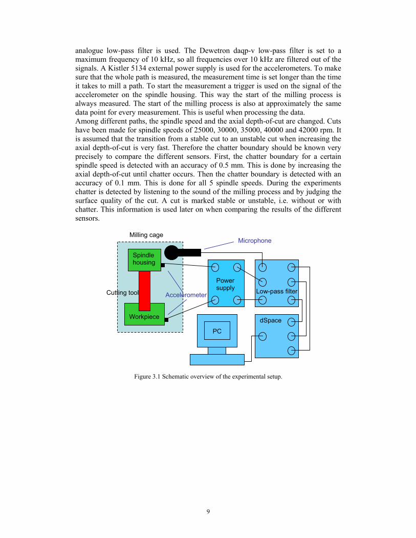
4.1 Data processing The data acquired from the experiments are plotted in a Power Spectral Density (PSD) plot. This frequency domain plot shows on the horizontal axis the frequency and on the vertical axis the power spectral density of the signal at these frequencies. The data processing is done with MATLAB. To make a useful PSD plot, some parameters should be adjusted well. The maximum frequency that can be derived from the signal is dependant on the sample frequency. In this case the sample frequency was 20000 Hz, so the maximum frequency that can be derived from these signals is 10000 Hz. The range of data points that should be analyzed should be determined. This is necessary because we want to analyse the milling process, not the spinning in the air of the cutting tool. The measured data contains both. Therefore, a time domain plot is made with on the horizontal axis the time in seconds and on the vertical axis the acceleration of the spindle housing, see figure 4.1. The time interval in which the milling process actually takes place can be seen very clearly. In this interval, the amplitude of the signal is much larger than outside this interval.

-0.5 0 0.5 1 1.5 2-200

-150

-100

-50

0

50

100

150

200

Time [s]

Acce

lera

tion

[m/s

2 ]

Figure 4.1 Time-domain signal of the accelerometer on the spindle housing at 25000 rpm and an axial

depth-of-cut of 4.5 mm. Another important parameter that should be adjusted is the number of frequencies that should be shown. The frequency resolution depends on the length of the time-domain window. This data window should not be too large. This causes a wide band of noise with only a few very small peaks on it. It should also not be chosen too small. This will cause a coarse line with only a few wide peaks in it. Most peaks will be averaged with surrounding frequencies and can therefore not be seen. A data window with 2048

11

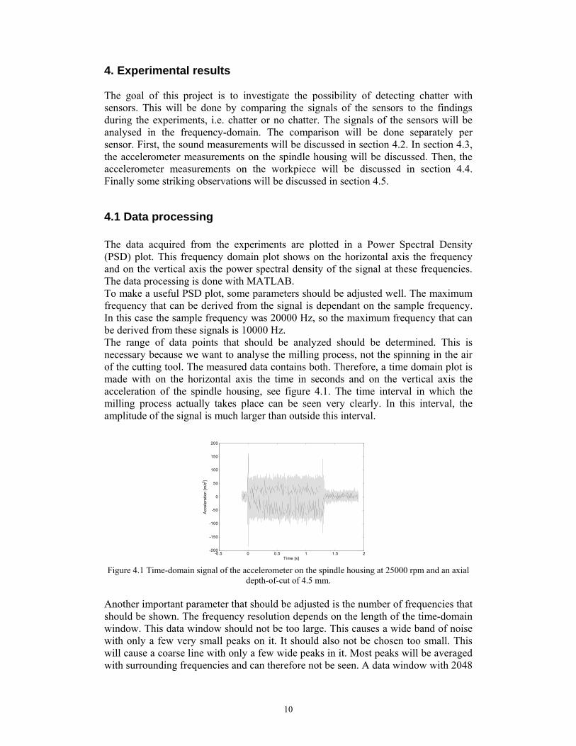
data points will give a good result, see Figure 4.2. When switching from time-domain to frequency-domain, a time-domain window should be used to avoid aliasing. In this case, a Hanning-window is used. Using these parameters a useful PSD plot can be made. Due to small roundness and alignment errors of the spindle and the cutting tool, it is expected to see the spindle speed frequency and multiples of the spindle speed frequency in the PSD plot. It is also expected to see multiples of the tooth passing frequency in the PSD plot because the cutting of a tooth is a periodic event. When chatter occurs in a cut, chatter will also be observed in the PSD plot. Not one, but a lot of chatter peaks will be seen because of the non-linearity of the system, described in section 2. So it is expected to see chatter peaks in pairs symmetrical around the multiples of the spindle speed and around the multiples of the tooth passing frequency [8]. It can be hard to determine whether a peak is a chatter peak or a peak resulting from the spindle speed or the tooth passing frequency. Since the spindle speed and the tooth passing frequency are known, these frequencies and their higher harmonics can be identified in the PSD by linear interpolation of the data. A circle is plotted at the multiples of the spindle speed frequency and an asterisk (*) is plotted at the multiples of the tooth passing frequency.

0 2000 4000 6000 8000 1000010-4

10-3

10-2

10-1

frequency [Hz]

Pow

er S

pect

ral D

ensi

ty [V

2 /Hz]

0 2000 4000 6000 8000 1000010-5

10-4

10-3

10-2

10-1

100

frequency [Hz]

Pow

er S

pect

ral D

ensi

ty [V

2 /Hz]

0 2000 4000 6000 8000 10000

10-10

10-5

100

frequency [Hz]

Pow

er S

pect

ral D

ensi

ty [V

2 /Hz]

Figure 4.2 Comparison of a PSD of a sound signal with too few, enough and too many data points.

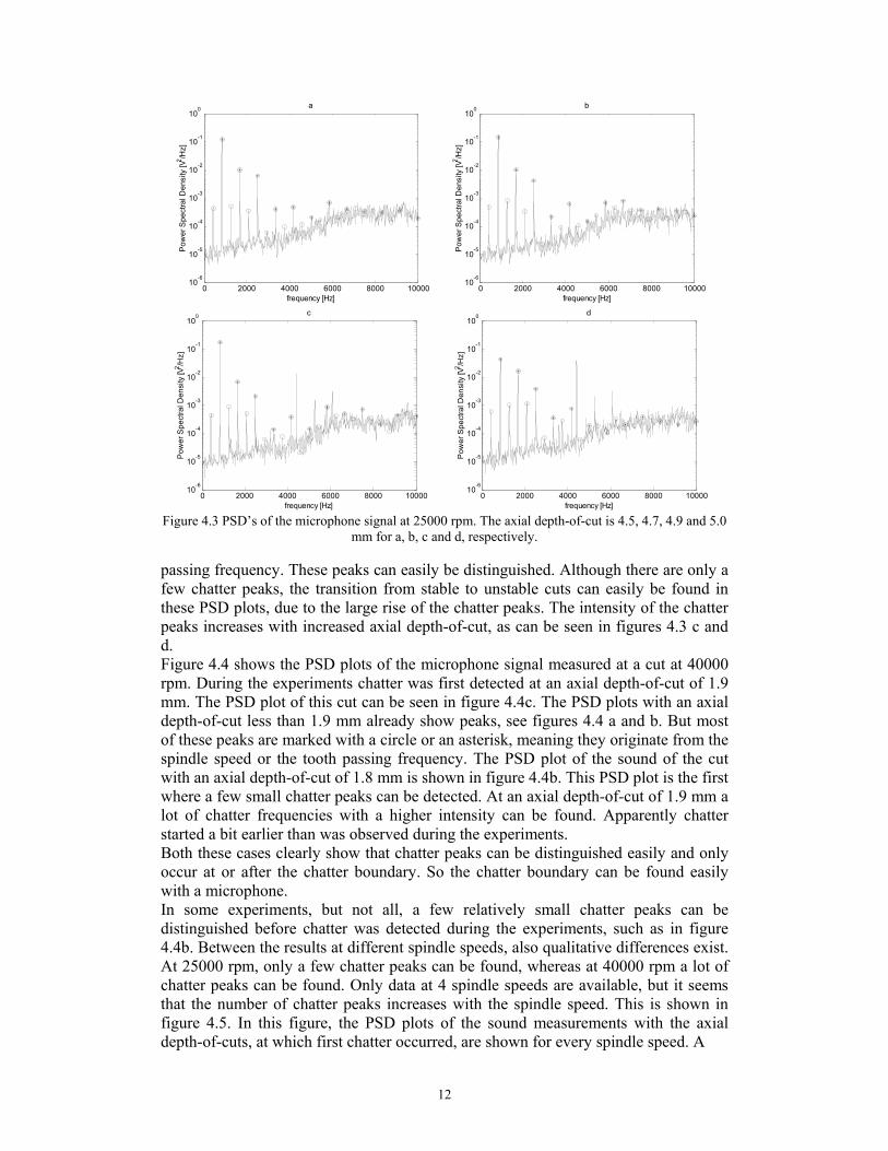
4.2 Sound measurements In this section, the results of the sound measurements will be discussed. All spindle speeds show a comparable development of the chatter peaks with increasing axial depth-of-cut. But there are also differences. Therefore, the results for two spindle speeds, 25000 and 40000 rpm, will be discussed to show the similarities but also the differences. The results at 42000 rpm differ significantly from the rest. Results for this spindle speed will be discussed later in a separate section. Because the microphone signal is measured in Volts and no calibration in terms of sound pressure is available, the unit of the PSD of the sound measurements will be V2/Hz. This has no effect on the analysis of the signal because the ratio of the values of the data points, and therefore also the ratio of the intensity of the frequencies, will stay the same. Figure 4.3 shows the PSD plots of the microphone signal measured at a cut at 25000 rpm. During the experiments chatter was first detected at an axial depth-of-cut of 4.9 mm. The PSD plot of this cut can be seen in figure 4.3c. The PSD plots with an axial depth-of-cut less than 4.9 mm already show peaks, see figures 4.3 a and b. These peaks are marked with a circle or an asterisk, meaning they originate from the spindle speed or the tooth passing frequency, respectively. The PSD plot shown in figure 4.3c is the first plot that has peaks that do not originate from the spindle speed or the tooth

12

0 2000 4000 6000 8000 1000010

-6

10-5

10-4

10-3

10-2

10-1

100

frequency [Hz]

Pow

er S

pect

ral D

ensi

ty [V

2 /Hz]

a

0 2000 4000 6000 8000 1000010

-6

10-5

10-4

10-3

10-2

10-1

100

frequency [Hz]

Pow

er S

pect

ral D

ensi

ty [V

2 /Hz]

b

0 2000 4000 6000 8000 1000010

-6

10-5

10-4

10-3

10-2

10-1

100

frequency [Hz]

Pow

er S

pect

ral D

ensi

ty [V

2 /Hz]

c

0 2000 4000 6000 8000 10000

10-6

10-5

10-4

10-3

10-2

10-1

100

frequency [Hz]

Pow

er S

pect

ral D

ensi

ty [V

2 /Hz]

d

Figure 4.3 PSD’s of the microphone signal at 25000 rpm. The axial depth-of-cut is 4.5, 4.7, 4.9 and 5.0

mm for a, b, c and d, respectively.

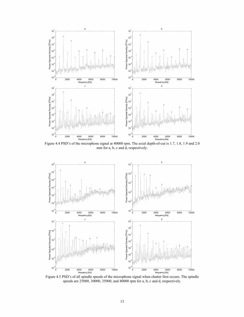
passing frequency. These peaks can easily be distinguished. Although there are only a few chatter peaks, the transition from stable to unstable cuts can easily be found in these PSD plots, due to the large rise of the chatter peaks. The intensity of the chatter peaks increases with increased axial depth-of-cut, as can be seen in figures 4.3 c and d. Figure 4.4 shows the PSD plots of the microphone signal measured at a cut at 40000 rpm. During the experiments chatter was first detected at an axial depth-of-cut of 1.9 mm. The PSD plot of this cut can be seen in figure 4.4c. The PSD plots with an axial depth-of-cut less than 1.9 mm already show peaks, see figures 4.4 a and b. But most of these peaks are marked with a circle or an asterisk, meaning they originate from the spindle speed or the tooth passing frequency. The PSD plot of the sound of the cut with an axial depth-of-cut of 1.8 mm is shown in figure 4.4b. This PSD plot is the first where a few small chatter peaks can be detected. At an axial depth-of-cut of 1.9 mm a lot of chatter frequencies with a higher intensity can be found. Apparently chatter started a bit earlier than was observed during the experiments. Both these cases clearly show that chatter peaks can be distinguished easily and only occur at or after the chatter boundary. So the chatter boundary can be found easily with a microphone. In some experiments, but not all, a few relatively small chatter peaks can be distinguished before chatter was detected during the experiments, such as in figure 4.4b. Between the results at different spindle speeds, also qualitative differences exist. At 25000 rpm, only a few chatter peaks can be found, whereas at 40000 rpm a lot of chatter peaks can be found. Only data at 4 spindle speeds are available, but it seems that the number of chatter peaks increases with the spindle speed. This is shown in figure 4.5. In this figure, the PSD plots of the sound measurements with the axial depth-of-cuts, at which first chatter occurred, are shown for every spindle speed. A

13

0 2000 4000 6000 8000 1000010

-6

10-5

10-4

10-3

10-2

10-1

100

101

frequency [Hz]

Pow

er S

pect

ral D

ensi

ty [V

2 /Hz]

a

0 2000 4000 6000 8000 10000

10-6

10-5

10-4

10-3

10-2

10-1

100

101

frequency [Hz]

Pow

er S

pect

ral D

ensi

ty [V

2 /Hz]

b

0 2000 4000 6000 8000 1000010

-6

10-5

10-4

10-3

10-2

10-1

100

101

frequency [Hz]

Pow

er S

pect

ral D

ensi

ty [V

2 /Hz]

c

0 2000 4000 6000 8000 10000

10-6

10-5

10-4

10-3

10-2

10-1

100

101

frequency [Hz]

Pow

er S

pect

ral D

ensi

ty [V

2 /Hz]

d

Figure 4.4 PSD’s of the microphone signal at 40000 rpm. The axial depth-of-cut is 1.7, 1.8, 1.9 and 2.0

mm for a, b, c and d, respectively.

0 2000 4000 6000 8000 1000010

-6

10-5

10-4

10-3

10-2

10-1

100

frequency [Hz]

Pow

er S

pect

ral D

ensi

ty [V

2 /Hz]

a

0 2000 4000 6000 8000 10000

10-6

10-5

10-4

10-3

10-2

10-1

frequency [Hz]

Pow

er S

pect

ral D

ensi

ty [V

2 /Hz]

b

0 2000 4000 6000 8000 1000010

-6

10-5

10-4

10-3

10-2

10-1

frequency [Hz]

Pow

er S

pect

ral D

ensi

ty [V

2 /Hz]

c

0 2000 4000 6000 8000 10000

10-6

10-5

10-4

10-3

10-2

10-1

100

101

frequency [Hz]

Pow

er S

pect

ral D

ensi

ty [V

2 /Hz]

d

Figure 4.5 PSD’s of all spindle speeds of the microphone signal when chatter first occurs. The spindle

speeds are 25000, 30000, 35000, and 40000 rpm for a, b, c and d, respectively.

14

possible explanation is that at high spindle speeds more power is needed. When chatter occurs, more power is available at high spindle speeds, resulting in more chatter peaks. The PSD’s of these experiments show that the intensity of the highest chatter peaks is always 1 to 10 times smaller than the intensity of the highest peaks originating from the spindle speed or tooth passing frequency. This could be a problem for automatic chatter detection. If a chatter frequency would have the largest intensity, the detection system could look at the highest peak. If the peak is not resulting from the spindle speed or the tooth passing frequency, it would be a chatter peak. But with the chatter peaks being smaller, this cannot be done. Here a filter is needed to filter out all the frequencies resulting from the spindle speed and the tooth passing frequency. Every peak that is left is a chatter peak. So if a good filter and an algorithm to detect peaks in the resulting signal can be made, then this is a good sensor for automatic chatter detection.

4.3 Accelerometer measurements on the spindle housing In this section the results of the measurements using the accelerometer on the spindle housing will be discussed. The results at two spindle speeds, 25000 and 40000 rpm, will be discussed. The development of the chatter peaks at 42000 rpm differs significantly from the other measurements. Results for this spindle speed will be discussed later in a separate section.

0 2000 4000 6000 8000 1000010

0

101

102

103

104

105

106

107

frequency [Hz]

Pow

er S

pect

ral D

ensi

ty [m

2 /(s4 *H

z)]

a

0 2000 4000 6000 8000 10000

100

101

102

103

104

105

106

107

frequency [Hz]

Pow

er S

pect

ral D

ensi

ty [m

2 /(s4 *H

z)]

b

0 2000 4000 6000 8000 1000010

0

101

102

103

104

105

106

107

frequency [Hz]

Pow

er S

pect

ral D

ensi

ty [m

2 /(s4 *H

z)]

c

0 2000 4000 6000 8000 10000

100

101

102

103

104

105

106

107

frequency [Hz]

Pow

er S

pect

ral D

ensi

ty [m

2 /(s4 *H

z)]

d

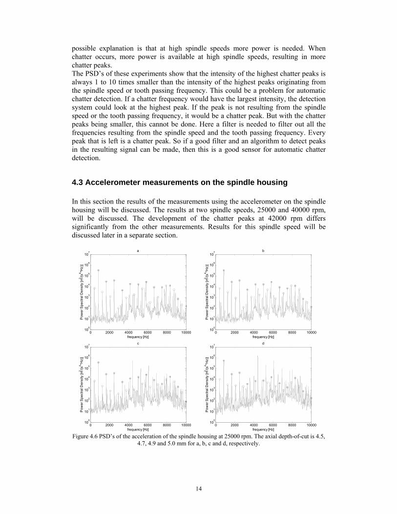
Figure 4.6 PSD’s of the acceleration of the spindle housing at 25000 rpm. The axial depth-of-cut is 4.5,

4.7, 4.9 and 5.0 mm for a, b, c and d, respectively.

15

0 2000 4000 6000 8000 1000010

1

102

103

104

105

106

107

frequency [Hz]

Pow

er S

pect

ral D

ensi

ty [m

2 /(s4 *H

z)]

a

0 2000 4000 6000 8000 10000

101

102

103

104

105

106

107

frequency [Hz]

Pow

er S

pect

ral D

ensi

ty [m

2 /(s4 *H

z)]

b

0 2000 4000 6000 8000 1000010

1

102

103

104

105

106

107

frequency [Hz]

Pow

er S

pect

ral D

ensi

ty [m

2 /(s4 *H

z)]

c

0 2000 4000 6000 8000 10000

101

102

103

104

105

106

107

frequency [Hz]

Pow

er S

pect

ral D

ensi

ty [m

2 /(s4 *H

z)]

d

Figure 4.7 PSD’s of the acceleration of the spindle housing at 40000 rpm. The axial depth-of-cut is 1.7,

1.8, 1.9 and 2.0 mm for a, b, c and d, respectively.

In figure 4.6, the PSD plots of the acceleration of the spindle housing for the cuts at 25000 rpm are shown. In figure 4.6b the results for the cut at 25000 rpm with an axial depth-of-cut of 4.7 mm are shown. This is the last stable cut found at 25000 rpm. The results for the first unstable cut are shown in figure 4.6c, with an axial depth-of-cut of 4.9 mm. What is immediately striking is that a large number of peaks, besides the ones originating from the spindle speed and tooth passing frequency, marked with a circle or an asterisk, respectively, can be observed, even before chatter has occurred. Some of these peaks come in pairs around a peak originating from the spindle speed or the tooth passing frequency, like the peaks between 8500 and 9000 Hz. The difference in frequency between most of the other chatter peaks and the spindle speed or tooth passing peaks is the same. This indicates that they originate from one frequency as explained in section 2. At the chatter boundary found during the experiments, these peaks do change a bit in frequency. This could indicate that the peaks before the chatter boundary come from a structural resonance frequency, and the peaks after the boundary from a chatter frequency as stated in section 2. The number of peaks and their intensity increase a bit with increasing axial depth-of-cut. The highest chatter peaks become higher than the highest peaks originating from the spindle speed or tooth passing frequency, making the chatter boundary clear. Figure 4.7 shows the PSD plots of the acceleration of the spindle housing for a cut at 40000 rpm. In figure 4.7b, the last stable cut is shown at an axial depth-of-cut of 1.8 mm. In figure 4.7c, the first unstable cut is shown at an axial depth-of-cut of 1.9 mm. A lot of peaks not originating from the spindle speed or tooth passing frequency can be observed before the chatter boundary has been crossed. After crossing this boundary the number and intensity of these peaks increases. In figure 4.8, the shift in frequency of the peaks at the chatter boundary is visualized for this spindle speed. Only a small frequency range is shown to make the shift more visible. This could

16

1.5 1.6 1.7 1.8 1.9 2 2.16800

7000

7200

7400

7600

7800

8000

8200

frequ

ency

[Hz]

depth of cut [mm]

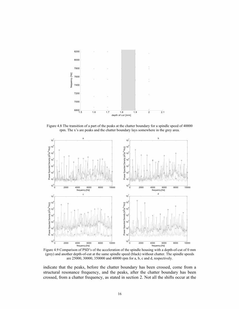
Figure 4.8 The transition of a part of the peaks at the chatter boundary for a spindle speed of 40000 rpm. The x’s are peaks and the chatter boundary lays somewhere in the grey area.

0 2000 4000 6000 8000 1000010

0

101

102

103

104

105

106

107

frequency [Hz]

Pow

er S

pect

ral D

ensi

ty [m

2 /(s4 *H

z)]

a

0 2000 4000 6000 8000 10000

100

101

102

103

104

105

106

107

frequency [Hz]

Pow

er S

pect

ral D

ensi

ty [m

2 /(s4 *H

z)]

b

0 2000 4000 6000 8000 1000010

0

101

102

103

104

105

106

107

frequency [Hz]

Pow

er S

pect

ral D

ensi

ty [m

2 /(s4 *H

z)]

c

0 2000 4000 6000 8000 10000

100

101

102

103

104

105

106

107

frequency [Hz]

Pow

er S

pect

ral D

ensi

ty [m

2 /(s4 *H

z)]

d

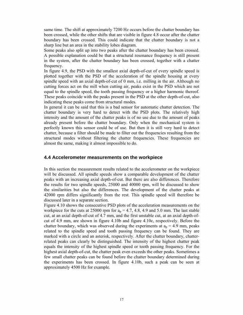
Figure 4.9 Comparison of PSD’s of the acceleration of the spindle housing with a depth-of-cut of 0 mm (grey) and another depth-of-cut at the same spindle speed (black) without chatter. The spindle speeds

are 25000, 30000, 350000 and 40000 rpm for a, b, c and d, respectively.

indicate that the peaks, before the chatter boundary has been crossed, come from a structural resonance frequency, and the peaks, after the chatter boundary has been crossed, from a chatter frequency, as stated in section 2. Not all the shifts occur at the

17

same time. The shift at approximately 7200 Hz occurs before the chatter boundary has been crossed, while the other shifts that are visible in figure 4.8 occur after the chatter boundary has been crossed. This could indicate that the chatter boundary is not a sharp line but an area in the stability lobes diagram. Some peaks also split up into two peaks after the chatter boundary has been crossed. A possible explanation could be that a structural resonance frequency is still present in the system, after the chatter boundary has been crossed, together with a chatter frequency. In figure 4.9, the PSD with the smallest axial depth-of-cut of every spindle speed is plotted together with the PSD of the acceleration of the spindle housing at every spindle speed with an axial depth-of-cut of 0 mm, i.e. milling in the air. Although no cutting forces act on the mill when cutting air, peaks exist in the PSD which are not equal to the spindle speed, the tooth passing frequency or a higher harmonic thereof. These peaks coincide with the peaks present in the PSD at the other depth-of-cut, also indicating these peaks come from structural modes. In general it can be said that this is a bad sensor for automatic chatter detection. The chatter boundary is very hard to detect with the PSD plots. The relatively high intensity and the amount of the chatter peaks is of no use due to the amount of peaks already present before the chatter boundary. Only when the mechanical system is perfectly known this sensor could be of use. But then it is still very hard to detect chatter, because a filter should be made to filter out the frequencies resulting from the structural modes without filtering the chatter frequencies. These frequencies are almost the same, making it almost impossible to do.

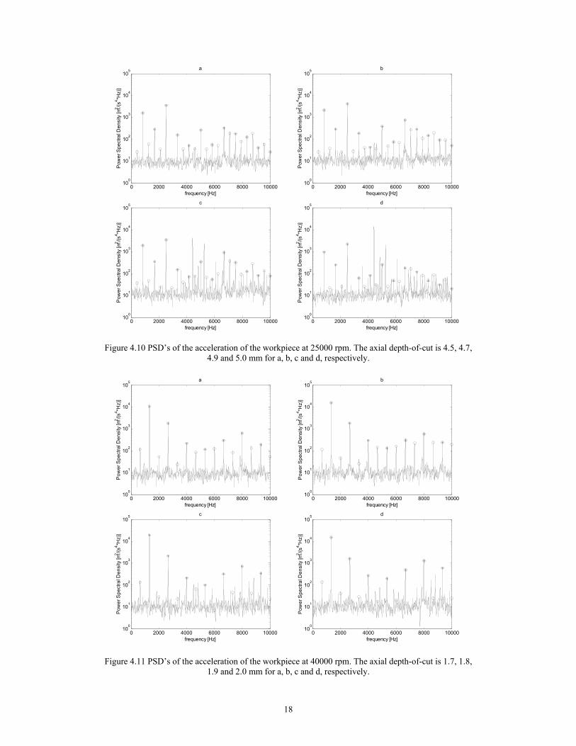
4.4 Accelerometer measurements on the workpiece In this section the measurement results related to the accelerometer on the workpiece will be discussed. All spindle speeds show a comparable development of the chatter peaks with an increasing axial depth-of-cut. But there are also differences. Therefore the results for two spindle speeds, 25000 and 40000 rpm, will be discussed to show the similarities but also the differences. The development of the chatter peaks at 42000 rpm differs significantly from the rest. This spindle speed will therefore be discussed later in a separate section. Figure 4.10 shows the consecutive PSD plots of the acceleration measurements on the workpiece for the cuts at 25000 rpm for ap = 4.7, 4.8, 4.9 and 5.0 mm. The last stable cut, at an axial depth-of-cut of 4.7 mm, and the first unstable cut, at an axial depth-of-cut of 4.9 mm, are shown in figure 4.10b and figure 4.10c, respectively. Before the chatter boundary, which was observed during the experiments at ap = 4.9 mm, peaks related to the spindle speed and tooth passing frequency can be found. They are marked with a circle and an asterisk, respectively. After the chatter boundary, chatter-related peaks can clearly be distinguished. The intensity of the highest chatter peak equals the intensity of the highest spindle speed or tooth passing frequency. For the highest axial depth-of-cut, the chatter peak even exceeds the other peaks. Sometimes a few small chatter peaks can be found before the chatter boundary determined during the experiments has been crossed. In figure 4.10b, such a peak can be seen at approximately 4500 Hz for example.

18

0 2000 4000 6000 8000 1000010

0

101

102

103

104

105

frequency [Hz]

Pow

er S

pect

ral D

ensi

ty [m

2 /(s4 *H

z)]

a

0 2000 4000 6000 8000 10000

100

101

102

103

104

105

frequency [Hz]

Pow

er S

pect

ral D

ensi

ty [m

2 /(s4 *H

z)]

b

0 2000 4000 6000 8000 1000010

0

101

102

103

104

105

frequency [Hz]

Pow

er S

pect

ral D

ensi

ty [m

2 /(s4 *H

z)]

c

0 2000 4000 6000 8000 10000

100

101

102

103

104

105

frequency [Hz]

Pow

er S

pect

ral D

ensi

ty [m

2 /(s4 *H

z)]

d

Figure 4.10 PSD’s of the acceleration of the workpiece at 25000 rpm. The axial depth-of-cut is 4.5, 4.7, 4.9 and 5.0 mm for a, b, c and d, respectively.

0 2000 4000 6000 8000 1000010

0

101

102

103

104

105

frequency [Hz]

Pow

er S

pect

ral D

ensi

ty [m

2 /(s4 *H

z)]

a

0 2000 4000 6000 8000 10000

100

101

102

103

104

105

frequency [Hz]

Pow

er S

pect

ral D

ensi

ty [m

2 /(s4 *H

z)]

b

0 2000 4000 6000 8000 1000010

0

101

102

103

104

105

frequency [Hz]

Pow

er S

pect

ral D

ensi

ty [m

2 /(s4 *H

z)]

c

0 2000 4000 6000 8000 10000

100

101

102

103

104

105

frequency [Hz]

Pow

er S

pect

ral D

ensi

ty [m

2 /(s4 *H

z)]

d

Figure 4.11 PSD’s of the acceleration of the workpiece at 40000 rpm. The axial depth-of-cut is 1.7, 1.8, 1.9 and 2.0 mm for a, b, c and d, respectively.

19

Figure 4.11 shows the PSD plots of the acceleration of the workpiece at 40000 rpm. At a depth-of-cut before the chatter boundary, only peaks originating from the spindle speed or tooth passing frequency can be seen, see figures 4.11a and b. At a depth-of-cut beyond the chatter boundary, determined during the experiment, some chatter peaks can be found with a low intensity compared to the spindle speed frequencies and the tooth passing frequencies. This is shown in figure 4.11c. Despite the low number of peaks and their small intensity, the chatter boundary can still be determined from these PSD plots. In general, the PSD plots of the acceleration of the workpiece show a small number of chatter peaks with a low intensity. In some rare cases, the intensity of a chatter frequency becomes 10 times larger than the highest spindle speed or tooth passing frequency. But usually, these peaks in the PSD remain 10 to 100 times smaller than those related to the spindle speed or the tooth passing frequency. The chatter boundary can be determined from the PSD plots. But because the chatter peaks in general do not exceed the spindle speed or tooth passing frequencies, a filter should be made as is the case for the microphone measurements. If such a filter can be made and an algorithm can be made to detect the remaining chatter frequencies, this sensor is suitable as a chatter detection sensor.

4.5 Striking phenomena In this section some striking phenomena, which occurred during the experiments and the analysis of the data, will be discussed. First the influence of the wall thickness between consecutive paths on the chatter boundary will be discussed in section 4.5.1. Then, in section 4.5.2, the starting and stopping of chatter halfway a path will be discussed. The development of wide peaks in a PSD plot with increasing depth-of-cut is analysed in section 4.5.3. Section 4.5.4 discusses the results of the sensors at a spindle speed of 42000 rpm.

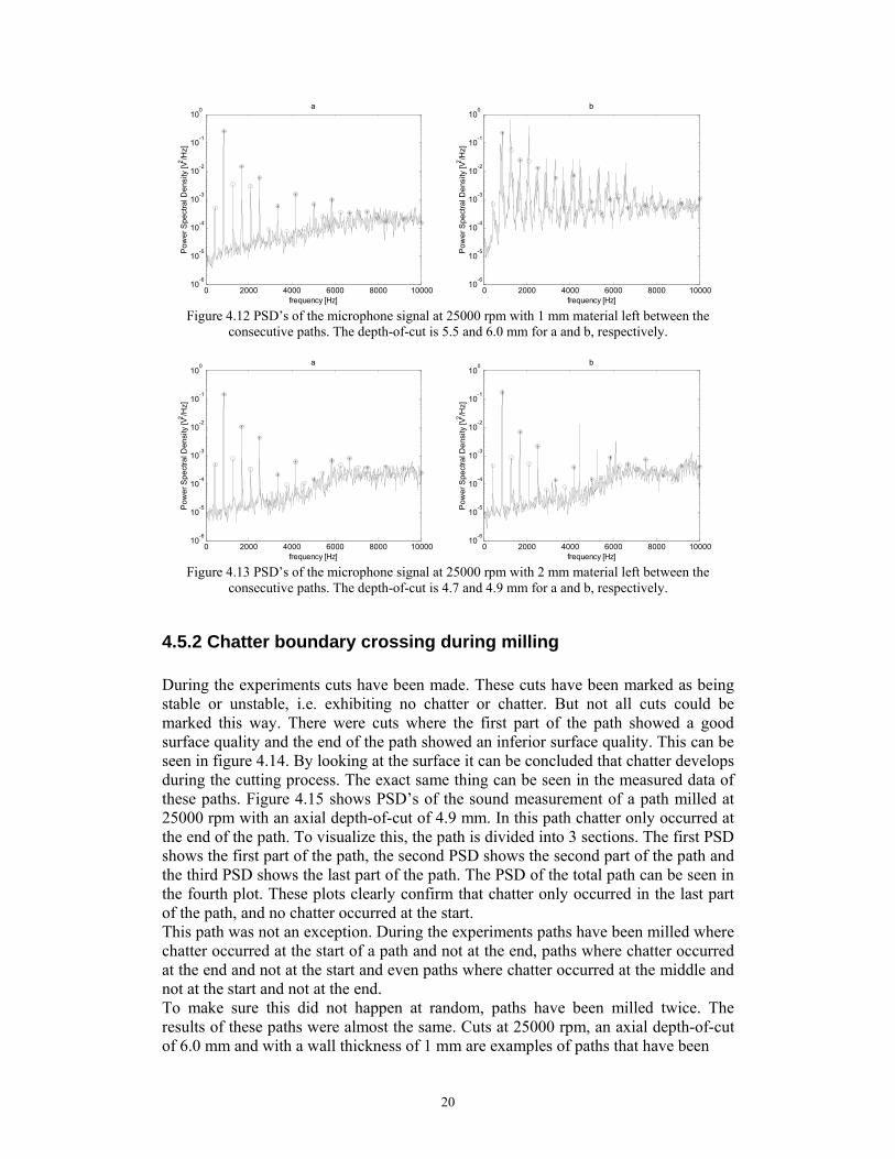
4.5.1 Influence of the wall thickness All the experiments are done with all process parameters kept constant within each path, as explained in section 3.2. Between the consecutive paths some material is left. At 25000 rpm cuts have been made with a wall thickness of 1 mm and 2 mm between the paths. This appears to be of great influence for the development of chatter. The decision whether or not a cut is marked as exhibiting chatter is based upon the surface quality and the sound of the cutting process. With 1 mm left, chatter occurs first between an axial depth-of-cut of 5.5 and 6 mm, as can be seen in figure 4.12. With 2 mm left, chatter already occurs between 4.7 and 4.9 mm, as can be seen in figure 4.13. The only thing that can cause this, is the reaction force of the material to the cutter. In no other way the cutter can ‘notice’ the difference between material of 1 or 2 mm at its side. The fact that chatter occurs earlier with more material at its side can be explained. The more material is left, the higher the reaction force will be. This causes chatter to develop earlier. This is an issue for further investigation in order to make models of the milling process more accurate.

20

0 2000 4000 6000 8000 1000010

-6

10-5

10-4

10-3

10-2

10-1

100

frequency [Hz]

Pow

er S

pect

ral D

ensi

ty [V

2 /Hz]

a

0 2000 4000 6000 8000 1000010

-6

10-5

10-4

10-3

10-2

10-1

100

frequency [Hz]

Pow

er S

pect

ral D

ensi

ty [V

2 /Hz]

b

Figure 4.12 PSD’s of the microphone signal at 25000 rpm with 1 mm material left between the

consecutive paths. The depth-of-cut is 5.5 and 6.0 mm for a and b, respectively.

0 2000 4000 6000 8000 1000010

-6

10-5

10-4

10-3

10-2

10-1

100

frequency [Hz]

Pow

er S

pect

ral D

ensi

ty [V

2 /Hz]

a

0 2000 4000 6000 8000 1000010

-6

10-5

10-4

10-3

10-2

10-1

100

frequency [Hz]

Pow

er S

pect

ral D

ensi

ty [V

2 /Hz]

b

Figure 4.13 PSD’s of the microphone signal at 25000 rpm with 2 mm material left between the

consecutive paths. The depth-of-cut is 4.7 and 4.9 mm for a and b, respectively.

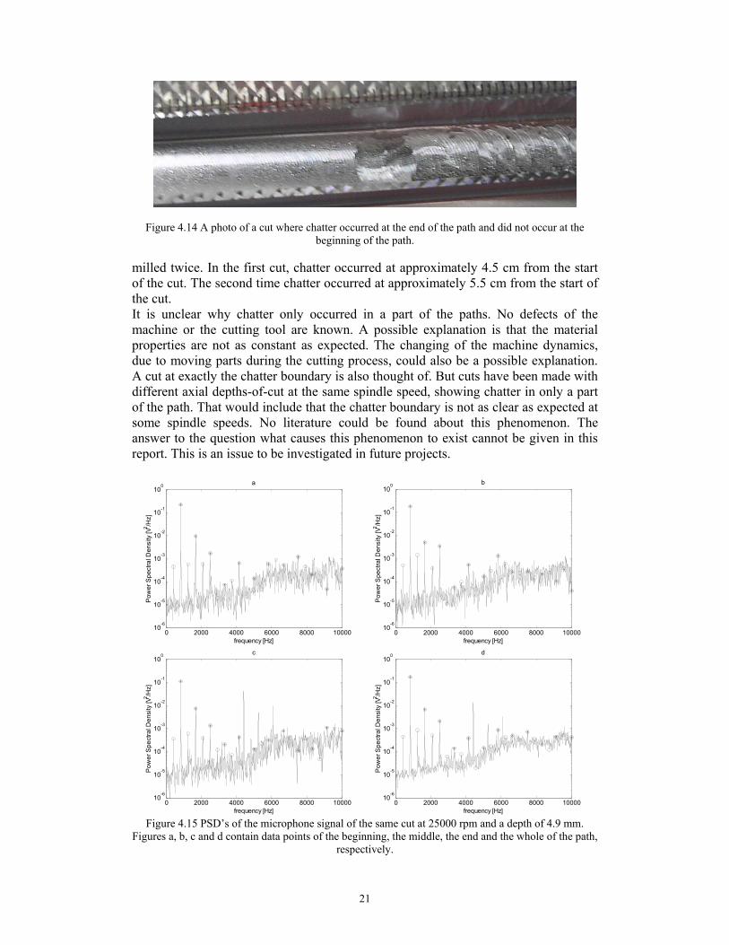
4.5.2 Chatter boundary crossing during milling During the experiments cuts have been made. These cuts have been marked as being stable or unstable, i.e. exhibiting no chatter or chatter. But not all cuts could be marked this way. There were cuts where the first part of the path showed a good surface quality and the end of the path showed an inferior surface quality. This can be seen in figure 4.14. By looking at the surface it can be concluded that chatter develops during the cutting process. The exact same thing can be seen in the measured data of these paths. Figure 4.15 shows PSD’s of the sound measurement of a path milled at 25000 rpm with an axial depth-of-cut of 4.9 mm. In this path chatter only occurred at the end of the path. To visualize this, the path is divided into 3 sections. The first PSD shows the first part of the path, the second PSD shows the second part of the path and the third PSD shows the last part of the path. The PSD of the total path can be seen in the fourth plot. These plots clearly confirm that chatter only occurred in the last part of the path, and no chatter occurred at the start. This path was not an exception. During the experiments paths have been milled where chatter occurred at the start of a path and not at the end, paths where chatter occurred at the end and not at the start and even paths where chatter occurred at the middle and not at the start and not at the end. To make sure this did not happen at random, paths have been milled twice. The results of these paths were almost the same. Cuts at 25000 rpm, an axial depth-of-cut of 6.0 mm and with a wall thickness of 1 mm are examples of paths that have been

21

Figure 4.14 A photo of a cut where chatter occurred at the end of the path and did not occur at the beginning of the path.

milled twice. In the first cut, chatter occurred at approximately 4.5 cm from the start of the cut. The second time chatter occurred at approximately 5.5 cm from the start of the cut. It is unclear why chatter only occurred in a part of the paths. No defects of the machine or the cutting tool are known. A possible explanation is that the material properties are not as constant as expected. The changing of the machine dynamics, due to moving parts during the cutting process, could also be a possible explanation. A cut at exactly the chatter boundary is also thought of. But cuts have been made with different axial depths-of-cut at the same spindle speed, showing chatter in only a part of the path. That would include that the chatter boundary is not as clear as expected at some spindle speeds. No literature could be found about this phenomenon. The answer to the question what causes this phenomenon to exist cannot be given in this report. This is an issue to be investigated in future projects.

0 2000 4000 6000 8000 1000010

-6

10-5

10-4

10-3

10-2

10-1

100

frequency [Hz]

Pow

er S

pect

ral D

ensi

ty [V

2 /Hz]

a

0 2000 4000 6000 8000 10000

10-6

10-5

10-4

10-3

10-2

10-1

100

frequency [Hz]

Pow

er S

pect

ral D

ensi

ty [V

2 /Hz]

b

0 2000 4000 6000 8000 1000010

-6

10-5

10-4

10-3

10-2

10-1

100

frequency [Hz]

Pow

er S

pect

ral D

ensi

ty [V

2 /Hz]

c

0 2000 4000 6000 8000 10000

10-6

10-5

10-4

10-3

10-2

10-1

100

frequency [Hz]

Pow

er S

pect

ral D

ensi

ty [V

2 /Hz]

d

Figure 4.15 PSD’s of the microphone signal of the same cut at 25000 rpm and a depth of 4.9 mm.

Figures a, b, c and d contain data points of the beginning, the middle, the end and the whole of the path, respectively.

22

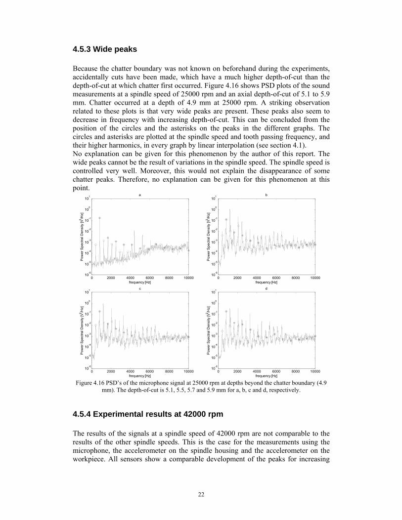
4.5.3 Wide peaks Because the chatter boundary was not known on beforehand during the experiments, accidentally cuts have been made, which have a much higher depth-of-cut than the depth-of-cut at which chatter first occurred. Figure 4.16 shows PSD plots of the sound measurements at a spindle speed of 25000 rpm and an axial depth-of-cut of 5.1 to 5.9 mm. Chatter occurred at a depth of 4.9 mm at 25000 rpm. A striking observation related to these plots is that very wide peaks are present. These peaks also seem to decrease in frequency with increasing depth-of-cut. This can be concluded from the position of the circles and the asterisks on the peaks in the different graphs. The circles and asterisks are plotted at the spindle speed and tooth passing frequency, and their higher harmonics, in every graph by linear interpolation (see section 4.1). No explanation can be given for this phenomenon by the author of this report. The wide peaks cannot be the result of variations in the spindle speed. The spindle speed is controlled very well. Moreover, this would not explain the disappearance of some chatter peaks. Therefore, no explanation can be given for this phenomenon at this point.

0 2000 4000 6000 8000 1000010

-6

10-5

10-4

10-3

10-2

10-1

100

101

frequency [Hz]

Pow

er S

pect

ral D

ensi

ty [V

2 /Hz]

a

0 2000 4000 6000 8000 10000

10-6

10-5

10-4

10-3

10-2

10-1

100

101

frequency [Hz]

Pow

er S

pect

ral D

ensi

ty [V

2 /Hz]

b

0 2000 4000 6000 8000 1000010

-6

10-5

10-4

10-3

10-2

10-1

100

101

frequency [Hz]

Pow

er S

pect

ral D

ensi

ty [V

2 /Hz]

c

0 2000 4000 6000 8000 10000

10-6

10-5

10-4

10-3

10-2

10-1

100

101

frequency [Hz]

Pow

er S

pect

ral D

ensi

ty [V

2 /Hz]

d

Figure 4.16 PSD’s of the microphone signal at 25000 rpm at depths beyond the chatter boundary (4.9

mm). The depth-of-cut is 5.1, 5.5, 5.7 and 5.9 mm for a, b, c and d, respectively.

4.5.4 Experimental results at 42000 rpm The results of the signals at a spindle speed of 42000 rpm are not comparable to the results of the other spindle speeds. This is the case for the measurements using the microphone, the accelerometer on the spindle housing and the accelerometer on the workpiece. All sensors show a comparable development of the peaks for increasing

23

depth-of-cut, taking the characteristics of each sensor into account. Therefore, only the sound measurements will be discussed in this section. In appendix A, the PSD’s of the signals from the microphone are shown. The axial depth-of-cut ranges from 2 mm to 5.6 mm. During the experiments chatter was first detected at an axial depth-of-cut of 5.4 mm. At an axial depth-of-cut of 2.0 mm no chatter peaks can be found. Only peaks originating from the spindle speed or the tooth passing frequency can be seen. At a depth-of-cut of 2.5 mm some chatter peaks can be detected. These peaks grow with increasing depth-of-cut. Between 3.5 and 4.0 mm the peaks suddenly disappear. No chatter peaks can be detected until chatter was first detected at 5.4 mm. After that, the chatter peaks increase in number and intensity. The development of the chatter peaks at 42000 rpm differs a lot from the other spindle speeds. First it looks like chatter occurs, then there is a region without chatter, and then chatter seems to occur again, at the depth at which chatter was detected during the experiments. The peaks in the second chatter region seem to be a bit wider for all sensors. First, period doubling was considered as a cause. This kind of chatter can cause a line in the stability lobes diagram with constant spindle speed to have two stable and two unstable regions. The chatter frequency of period doubling is half the tooth passing frequency. In the experiments a cutter with two cutting edges is used. So the chatter peaks would coincide with the spindle speed peaks. That is not the case. There are chatter peaks visible in the PSD plots, making period doubling impossible as a cause. Another explanation that could cause a line in the stability lobes diagram with constant spindle speed to have two stable and two unstable regions can not be given. Further investigation is recommended to find the cause for this phenomenon.

24

5. Conclusions and recommendations In this report, the sensor choice for chatter detection in high-speed milling applications has been investigated. Several sensors have been compared by comparing the results of dedicated experiments. The sensors that were compared are a microphone, an accelerometer on the spindle housing and an accelerometer on the workpiece. From this comparison, the microphone has been shown to be the best sensor to detect chatter in high-speed milling applications. In the PSD of the microphone signal, the chatter boundary can be clearly detected. When no chatter occurs, there are no peaks in the signal, except the peaks resulting from the spindle speed and the tooth passing frequency. When chatter occurs, extra peaks are present in the signal. On average there are quite a few of these peaks with a high intensity. The accelerometer on the spindle housing always had peaks not resulting from the spindle speed or tooth passing frequency in its signal. These extra peaks make it almost impossible to determine the chatter boundary. The accelerometer on the workpiece can also be used to determine chatter. The development of the chatter peaks in the signal of this sensor is comparable to the development of the chatter peaks in the signal of the microphone, except that there are on average fewer peaks with a lower intensity, on which the chatter detection can be based. Considering all these observations, the accelerometer on the workpiece and the microphone are both useful sensors, but the microphone is better suited for chatter detection in high-speed milling applications. Further investigation in the use of audio signals is needed for automated chatter detection and control. The properties of chatter detection with a microphone in a noisy environment should be investigated. Adaptive filtering and noise cancellation techniques should be considered to improve the usefulness of the microphone as a chatter detection sensor. During the experiments and the analysis of the results, some unknown phenomena have been observed, making it harder to detect the chatter boundary. Some of these peculiarities should be subjects for further investigation. Especially the fact that chatter occurred only in a part of a milled path deserves further attention. Furthermore, it is unknown what the reason is for wide peaks, after the chatter boundary has been crossed. These two subjects should be considered in further research.

25

References [1] Y. Altintas, Manufacturing automation, Cambridge University Press, 2000. [2] Y. Altintas, Machine tool dynamics and vibrations. In: O.D.I. Nwokah, Y.

Hurmuzlu (editors), The mechanical system design handbook – modeling, measurement and control, chapter 4, CRC Press, 2002.

[3] M.A. Davies, T.J. Burns, C.J. Evans, On the dynamics of chip formation in machining hard materials, CIRP Annals (46): 25-30, 1997.

[4] T. Delio, J. Tlusty, S. Smith, Use of audio signals for chatter detection and control, Journal of Engineering for Industry, transactions of the ASME, 114: 146-157, 1992.

[5] R.P.H. Faassen, N. van de Wouw, J.A.J. Oosterling, H. Nijmeijer, Prediction of regenerative chatter by modelling and analysis of high-speed milling, International Journal of Machine Tools & Manufacture, 43: 1437-1446, 2003.

[6] R.P.H. Faassen, N. van de Wouw, J.A.J. Oosterling, H. Nijmeijer, Modelling the high-speed milling process for chatter prediction, in 24th Benelux Meeting on Systems and Control; Editors: Catoire, L., Kinnaert, M. and Vande Wouwer, A., Houffalize, Belgium, 76, 2005.

[7] I. Grabec, Chaotic dynamics of the cutting process, International Journal of Machine Tools & Manufacture, 28:19-32, 1988.

[8] T.Insperger, G. Stépán, P.V. Bayly, B.P. Mann, Multiple chatter frequencies in milling processes, Journal of Sound and Vibration, 262: 333-345, 2003.

[9] J. Tlusty, Manufacturing processes and equipment, Prentice Hall, 2000. [10] M. Wiercigroch, E. Budak, Sources of nonlinearities, chatter generation and

suppression in metal cutting, Philosophical Transactions of the Royal Society of London, 359 (A): 663-693, 2001.

[11] M. Wiercigroch, A.M. Krivtsov, Frictional chatter in orthogonal metal cutting, Philosophical Transactions of the Royal Society of London, 359 (A): 713-738, 2001.

26

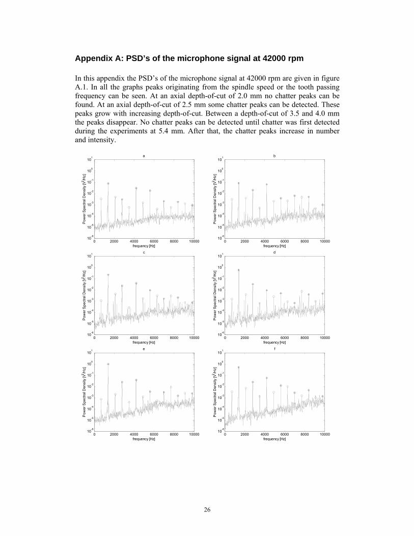
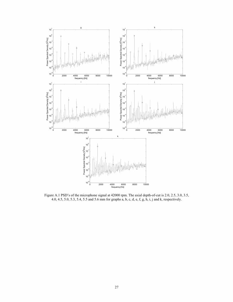
Appendix A: PSD’s of the microphone signal at 42000 rpm In this appendix the PSD’s of the microphone signal at 42000 rpm are given in figure A.1. In all the graphs peaks originating from the spindle speed or the tooth passing frequency can be seen. At an axial depth-of-cut of 2.0 mm no chatter peaks can be found. At an axial depth-of-cut of 2.5 mm some chatter peaks can be detected. These peaks grow with increasing depth-of-cut. Between a depth-of-cut of 3.5 and 4.0 mm the peaks disappear. No chatter peaks can be detected until chatter was first detected during the experiments at 5.4 mm. After that, the chatter peaks increase in number and intensity.

0 2000 4000 6000 8000 1000010

-6

10-5

10-4

10-3

10-2

10-1

100

101

frequency [Hz]

Pow

er S

pect

ral D

ensi

ty [V

2 /Hz]

a

0 2000 4000 6000 8000 10000

10-6

10-5

10-4

10-3

10-2

10-1

100

101

frequency [Hz]

Pow

er S

pect

ral D

ensi

ty [V

2 /Hz]

b

0 2000 4000 6000 8000 1000010

-6

10-5

10-4

10-3

10-2

10-1

100

101

frequency [Hz]

Pow

er S

pect

ral D

ensi

ty [V

2 /Hz]

c

0 2000 4000 6000 8000 10000

10-6

10-5

10-4

10-3

10-2

10-1

100

101

frequency [Hz]

Pow

er S

pect

ral D

ensi

ty [V

2 /Hz]

d

0 2000 4000 6000 8000 1000010

-6

10-5

10-4

10-3

10-2

10-1

100

101

frequency [Hz]

Pow

er S

pect

ral D

ensi

ty [V

2 /Hz]

e

0 2000 4000 6000 8000 10000

10-6

10-5

10-4

10-3

10-2

10-1

100

101

frequency [Hz]

Pow

er S

pect

ral D

ensi

ty [V

2 /Hz]

f

27

0 2000 4000 6000 8000 1000010

-6

10-5

10-4

10-3

10-2

10-1

100

101

frequency [Hz]

Pow

er S

pect

ral D

ensi

ty [V

2 /Hz]

g

0 2000 4000 6000 8000 10000

10-6

10-5

10-4

10-3

10-2

10-1

100

101

frequency [Hz]

Pow

er S

pect

ral D

ensi

ty [V

2 /Hz]

h

0 2000 4000 6000 8000 1000010

-6

10-5

10-4

10-3

10-2

10-1

100

101

frequency [Hz]

Pow

er S

pect

ral D

ensi

ty [V

2 /Hz]

i

0 2000 4000 6000 8000 10000

10-6

10-5

10-4

10-3

10-2

10-1

100

101

frequency [Hz]

Pow

er S

pect

ral D

ensi

ty [V

2 /Hz]

j

0 2000 4000 6000 8000 1000010

-6

10-5

10-4

10-3

10-2

10-1

100

101

frequency [Hz]

Pow

er S

pect

ral D

ensi

ty [V

2 /Hz]

k

Figure A.1 PSD’s of the microphone signal at 42000 rpm. The axial depth-of-cut is 2.0, 2.5, 3.0, 3.5, 4.0, 4.5, 5.0, 5.3, 5.4, 5.5 and 5.6 mm for graphs a, b, c, d, e, f, g, h, i, j and k, respectively.