Embed Size (px)
Citation preview
Chasing the Key Player:
A Network Approach to the Myanmar Civil War
Andrea Di Miceli*
This Version: December 1, 2016. For the latest version click here
Abstract
I study the determinants of civil conflict in Myanmar. As governments in weak states often face
several armed groups, they have to strategically allocate resources to fight a subset of them. I
use a simple model to embed heterogeneity among rebel groups stemming from their network
of alliances and enmities. The key insight is that, by attacking a group, the Myanmar army
weakens its allies. Therefore, the model predicts that the Myanmar army strategically targets
armed groups who are central in the network of alliances. To test the model’s predictions, I
collect a new data set on rebel groups’ locations, alliances, and enmities for the period 1989-
2015. Using geo-referenced information on armed groups attacked by the Myanmar army, the
empirical evidence strongly supports the predictions of the model. A one standard deviation
increase in a group’s centrality increases the likelihood of conflict with the Myanmar’s army by
1.2% (over a baseline yearly conflict probability of 6.4%), thus identifying a new determinant
of conflict. This result is robust to variables measuring the opportunity cost of conflict such as
rainfall and commodity price shocks. Since past (and expected) conflicts might affect alliances
and enmities between armed groups, I pursue an instrumental variable strategy to provide ev-
idence that the mechanism proposed is indeed causal.
JEL Classification: D74, F54, P48, O13.
Keywords: Civil Conflict, Network of Alliances, Myanmar, State Formation, Resource Curse,
Bargaining Failures, Ethnicity.
*UCLA Anderson School of Management, CCPR, e-mail: [email protected], I thank my advis-
ers Paola Giuliano and Romain Wacziarg, as well as my Ph.D. committee members Christian Dippel, Nico Voigtländer
for their outstanding guidance and support. I am grateful to Omer Ali, Sarah Brierley, Darin Christensen, Quoc-Anh
Do, Andreas Gulyas, Vasily Korovkin, Horacio Larreguy, Shekhar Mittal, George Ofosu, Mikhail Poyker, Shuyang
Sheng for several comments and suggestions that substantially improved this paper. I also thank seminar partic-
ipants at All-UC History Winter 2016 Conference in UC Irvine, Bruneck Workshop on The Political Economy of
Federalism and Local Development. Funding from the International Growth Center (project code 89402) at the
London School of Economics is gratefully acknowledged. All remaining errors are my own.

1 Introduction
Governments in weak states often face more than one armed group opposing their efforts to mo-
nopolize violence. Data show that in more than 90% of countries experiencing civil war govern-
ments have had two or more distinct armed groups to fight.1 This fact implies that a government
embroiled in civil war faces a complex decision on allocating resources to fight enemies. Recent
theoretical work has shed light on the incentives for a central government to consolidate power
depending on the characteristics of armed groups (Powell [2013]). However, the empirical litera-
ture has suffered from the lack of data and methodology that embeds armed groups’ heterogeneity
in a tractable framework yielding testable predictions.
In this study, I analyze the choice of the central government to attack rebels in its periphery.
To do so, I focus on the longest civil war of the contemporary period: the Myanmar conflict. The
country represents an ideal environment to study how its central government’s army, henceforth
denoted with its anglicized Burmese name of Tatmadaw, uses conflict to expand control over its
vast frontier. In fact, the Myanmar civil war is an attempt to consolidate power in which the Tat-
madaw faces multiple enemies at the same time.
I provide empirical evidence showing that the decision of the Myanmar army to attack a par-
ticular armed group is based on the complex web of alliances and enmities that exist between
armed groups. This mechanism relies on the idea that the ability of armed groups to withstand
a military offensive from the Tatmadaw increases in the number of allies and decreases the more
enemies an armed group has. Therefore, attacking an armed group has two effects: it weakens
the group itself (direct effect), but it also weakens its allies and emboldens its enemies (indirect
effect). The interplay of these two effects drives the Myanmar army’s decision of which groups to
attack over time. I use the observed cross-sectional and longitudinal variation in armed groups
alliances and enmities to test predictions from the model. Namely, a network statistic summarizes
which groups are more likely to be attacked in light of their network of alliances and enmities.
The network statistic is the key explanatory variable in an OLS regression that sheds light on the
attacks of the Tatmadaw against armed groups in the period 1989-2015.
Figure 1 shows the yearly variation in the top two armed groups attacked by the Myanmar
army and their respective number of conflict events during the period 1989-2015 (there are forty-
seven active armed groups over this period). The patterns of Figure 1 are in line with two stylized
facts of civil wars which are: (i) there are periods of persistent fighting and, (ii) fighting some-
times recurs after periods of peace.2 This evidence further supports analyzing Myanmar as a
representative case study.
My empirical analysis is derived from the predictions of a formal model. I take the onset of
civil war as given and use a model to better understand how the Tatmadaw targets its fighting
1This statistic has been computed using data covering the period 1989-2015 from the UCDP/PRIO Database[Croicu & Sundberg, 2015].
2See Powell [2012] for a discussion on the stylized facts of civil wars.
1

Figure 1: Yearly Variation in the Top Two Armed Groups Fought by the Myanmar Army
010
2030
4050
60Y
early
Con
flict
Eve
nts
1990
1995
2000
2005
2010
2015
KNU KNPP SUA KIO MNDAARCSS PSLF DKBA 5 UWSA
Source: UCDP 3.0 Georeferenced Event Dataset and Myanmar Peace Center Records.The armed groups in the picture are, respectively, the Karen National Union (KNU),Shan United Army (SUA), Myanmar National Democratic Army (MNDAA), PalaungState Liberation Front (PSLF), Karenni National Progressive Party (KNPP), Kachin In-dependence Organization (KIO), Restoration Council of Shan State (RCSS), United WaState Army (UWSA), Democratic Karen Benevolent Army (DKBA 5).
effort. In the model, the Myanmar army faces several armed groups with heterogeneous fighting
capacity. The fighting capacity of a group represents its ability to withstand an offensive from the
Tatmadaw. Every armed group is a node in the network of alliances and enmities.3 The fighting
capacity of a group is rooted in the network structure through alliances and enmities in a fashion
similar to Ballester, Calvó-Armengol & Zenou [2006]. Namely, the fighting capacity of a rebel
group increases in the fighting capacity of its allies and decreases in the fighting capacity of its
enemies. Historical evidence shows that alliances benefit a group’s fighting capacity in several
ways: allies provide supply lines for weapons, guarantee shelter outside a group’s territory dur-
ing offensives from the Myanmar army, and allies are often trading partners. Historical records
and anecdotes confirm that the Myanmar army is aware of the network structure. I capture this
insight by modeling the Tatmadaw’s choice of which armed group to attack according to an opti-
mal rule that takes into account the network structure between armed groups. The optimal rule
is to remove an armed group so as to reduce the overall fighting capacity of all armed groups in
the network. For instance, attacking an armed group who is the main weapons’ provider to other
armed groups inherently damages the overall fighting capacity in the network. In particular, I
3In every period, armed groups observe the network structure and non-cooperatively maximize their fightingcapacity.
2

use the network statistic called intercentrality that measures, for each armed group, the combined
direct and indirect effect on the overall fighting ability associated with their removal from the
network.4 The model predicts that the Myanmar army targets groups with higher intercentrality
parameter.
To derive predictions from the model and explain the pattern of violent outbreaks in Fig-
ure 1, I collected a new dataset of armed groups’ individual characteristics from various sources
documenting their alliances and enmities from 1989 until 2015. The network displays both cross-
sectional as well as temporal variation. I organize the empirical analysis in two steps. In the first
step, I show a positive and robust correlation between armed groups’ intercentrality and conflict
through a linear probability model. In the second step, I address identification concerns through
an instrumental variables (IV) estimation.
I use information on armed groups attacked by the Myanmar army and the location of clashes
available for the period 1989-2015 from the UCDP Georeferenced Event Dataset ([Croicu & Sund-
berg, 2015]) and Myanmar newspapers’ records. I identify the effect of a group’s intercentrality
on conflict from the longitudinal and cross-sectional variation in the network of armed groups.
Results based on a linear probability model show that a one standard deviation increase in a
group’s intercentrality over a year increases the expected probability of violence in any of its cells
by 1.2 percentage points over a baseline annual probability of 6.4%. This effect is highly signifi-
cant and robust to the inclusion of variables affecting the opportunity cost of fighting. To control
for geographical shocks that may influence the incentive to fight, I collect data on territories con-
trolled by armed groups, on natural resources therein and rainfall variation over time. All these
variables are relevant in the context of Myanmar, a country rich in natural resources that relies
mostly on rain-fed agriculture.5
The main concern affecting the proposed identification strategy is that the positive correlation
between a group’s intercentrality and attacks by the Tatmadaw might be driven by unobservable
characteristics that vary systematically at the armed group level. Moreover, past conflict (or the
expectation of future conflict) can lead a group to form (or strategically break) its alliances, in
which case there is reverse causality. I pursue an IV estimation to address identification concerns
and provide evidence that the positive relation between intercentrality and conflict is indeed
causal.
The IV estimation is implemented in three steps. In the first step, I predict a counterfactual
4The intercentrality measure is strictly related to the Katz-Bonacich network centrality [Bonacich, 1987]. Thiscentrality measure counts the number of all paths stemming from a given node, weighted by a decay factor. Intu-itively, it is a measure of information diffusion over the network, nodes with higher Bonacich centrality can spreadmore information over the network.
5In examining the determinants of civil wars, variables affecting the opportunity cost of fighting have receivedconsiderable attention. Several studies have shown that weather shocks are correlated with outbreaks of violencein regions that rely on rain-fed agriculture. Recent contributions to this topic are: Harari & La Ferrara [2015] andVanden Eynde [2016]. For a recent review see [Burke, Hsiang & Miguel, 2015]. Similarly, shocks to the price ofcommodities have been used to investigate their causal effects on conflict.See [Bazzi & Blattman, 2014], Berman &Couttenier [2013] as well as Dube & Vargas [2013], and Besley & Persson [2011] for recent studies reaching differentconclusions on the effect of commodity price shocks on conflict.
3

network structure using only exogenous variables that are not affected by past conflict. In the
second step, I compute the intercentrality parameter from this counterfactual network. In the
third step, I use the counterfactual intercentrality parameter as an instrument for the observed
one to implement a two-stage least squares (2SLS) estimation. Since the intercentrality is a non-
linear function of the network structure, the 2SLS estimation allows me to control transparently
for variables that directly impact both conflict and the observed network structure.
In the first step of the IV estimation, I use an empirical model of network formation to predict
a counterfactual network that is not affected by omitted variables bias.6 That is, I assume that
the observed relationships between armed groups stem from the maximization of their joint util-
ity. The network formation model estimates the parameters explaining the decision to form or
break alliances (as well as enmities and neutral relationships) over time. Therefore, the estimated
parameters are used to predict the counterfactual network over time. Variables included in the
network formation model are of two types: pre-determined and time varying. Pre-determined
characteristics such as the distance between ethnic homelands and linguistic proximity enter the
network formation model and play a major role in explaining the decision to form an alliance (or
an enmity). However, these variables are fixed over time and therefore cannot explain the longi-
tudinal variation in the network structure. To ensure that the counterfactual network structure
varies over time, I use fluctuations in the world price of resources within groups’ ethnic home-
lands. I argue that the value of forming an alliance (or an enmity) shifts over time because fluctu-
ations in the value of resources within ethnic homelands drive the incentives of armed groups to
form and break alliances motivated by trading interests. For instance, rebel groups whose ethnic
homelands have copper but lack access to the border might find profitable to form an alliance to
transport the commodity from their ethnic homelands outside the country once its price is suffi-
ciently high.
In the second step, I compute the intercentrality parameter of the counterfactual network.
Given the extensive evidence on the direct impact of resources on conflict, the empirical network
formation model raises the concern that these variables are not excludable when estimating the
network structure (because they might also have a direct impact on the probability of conflict).
However, the non-linear nature of the intercentrality parameter allows the inclusion of resources’
presence and their fluctuations when estimating the 2SLS. Therefore, the 2SLS estimation con-
trols for variables that might have a direct impact on the probability of conflict.
Estimates from the IV confirm the prediction of the model and the magnitude of the OLS
findings: a one standard deviation increase in an armed group’s instrumented intercentrality is
associated with an increase in the expected probability of violence occurring in its territory by
1.36 percentage points over a year. That is, the Tatmadaw takes into consideration the complex
web of alliances when deciding which group to attack during the last twenty-seven years. More-
over, the mechanism presented has a sizable impact on conflict when compared with the effects of
6The empirical model follows the contribution of Graham [2015].
4

weather and commodities’ shocks. The expected increase in the probability of conflict caused by a
one standard deviation increase in a group’s intercentrality is more than twice the effect observed
for a one standard deviation increase in teak wood price, the commodity with the most sizable
impact on conflict in the data. Similarly, the effect of a drought is roughly eighty percent the size
of a standard deviation increase of a group’s intercentrality.
This paper contributes to the literature studying the determinants of civil war. The impor-
tance of alliances and enmities in conflict has been highlighted by König, Rohner, Thoenig &
Zilibotti [2016] who show the effect of inter-group relationships in escalating or reducing conflict
during the Congo civil war. In my analysis, alliances and enmities between armed groups are
motivated by trading patterns and mutual economic interests that go beyond military assistance
on the battlefield. Therefore, this paper differs from theirs as it studies how the heterogeneity in
the network of alliances (and enmities) generates an incentive for the Myanmar army to attack
only some of the several armed groups present in the country.
The findings in this article contribute to the study of civil war as a tool for power consolida-
tion. In his recent theoretical contribution, Powell [2013] argues that both peaceful and violent
power consolidation are optimal choices of a dynamic bargaining game in which the government
aims to extend its monopoly of violence over a rebel group. The author contends that the gov-
ernment’s choice to peacefully buying off the rebel group rather than fighting it depends on the
individual characteristics of the group such as the presence of resources in its homeland and its
military strength. I argue that, by providing a simple framework that embeds armed groups’ het-
erogeneity, this paper shows preliminary evidence that conflict is the result of a rational decision
process in line with the one described by Powell [2013]. While the effort to control the nation’s
peripheries is at the core of state formation, this process has often occurred in the remote past
or in polities in which the absence of data impeded a formal analysis (Tilly [1985]).7 This paper
provides evidence on how this process developed during the last three decades in Myanmar.
Since Myanmar has more than one hundred ethnic groups, this work is also of interest to the
literature debating the role of ethnicity in conflict. In the empirical model of network formation,
I show that linguistically similar groups are likely not to be neutral to each other. This evidence is
consistent with findings showing that more closely related populations are more likely to engage
in conflict (Spolaore & Wacziarg [2016]) as well as with papers showing that ethnic polarization
might lead to conflict Esteban, Mayoral & Ray [2012].
The remainder of the paper is organized as follows: section 2 provides background informa-
tion on the Myanmar context, the model is presented in section 3. Section 4 discusses how the
dataset was built and section 5 shows correlations and discusses the identification problems. Sec-
tion 6 discusses the logic behind the IV and shows that estimates are consistent with OLS ones.
Section 7 summarizes the findings, discusses external validity and concludes.
7On the lack of data to study state formation see also Scott [2009]. Sánchez de la Sierra [2016] is a notableexception as it studies the incentives leading to embryonic state formation during the great Congo War. My work iscomplimentary to his because investigates the use of conflict for the purpose of power consolidation.
5

2 Background: Civil War in Myanmar
Only the Tatmadaw is mother,Only the Tatmadaw is father,Don’t believe what the surroundings say,Whoever tries to split us, we shall never split.We shall unite forever.8
Myanmar is a country located in South-East Asia; its land mass is comparable to Texas. The coun-
try’s borders are virtually the same since the British colonized it in 1886. As shown in Figure
2, Myanmar’s location is strategically important as it borders the two South Asian countries of
Bangladesh and India on its west side as well as China on its North-East. The country is also con-
nected to Laos to the east and shares the entirety of its Southeast border. Myanmar is ethnically
diverse which can be gauged from the variety of languages spoken therein (Figure 2). The Bamar
(or Burmese), depicted in yellow in Figure 2, are the country’s dominant ethnic group making up
roughly sixty-five percent of the total population. The Bamar occupy the core of the country while
more than one hundred and thirty ethnic groups live in its vast “periphery”.9 In what follows, I
detail the evolution of the civil war with a particular focus on the period between 1989 and 2015
as this is the time frame of interest for the empirical analysis.10
Myanmar obtained independence from the British in 1948. In the immediate aftermath, the
country experienced all different forms of intergroup violence. In fact, the Communist Party of
Burma (mostly made up of ethnic Bamar) rebelled shortly after independence while the first eth-
nic group to revolt against the central government were the Karen in 1949. Moreover, the country
was also invaded by the remnants of Yunnan’s Kuomintang in 1950. The constant threats and
the multiplicity of internal and external enemies caused the Tatmadaw’s power to grow up to the
point where the army was de facto substituting the elected government. In 1962, General Ne Win,
the highest ranked army official, seized power and ruled the country through a one-party state
until 1988.
Following the coup, the Tatmadaw entirely disenfranchised the non-Bamar ethnic groups,
causing the sprawling of ethnic armed groups. Indeed, many border areas were (and in many
cases still are) under control of ethnic armed groups with the Tatmadaw being unable to access
them. In regions where Bamar do not represent the ethnic majority the Tatmadaw controls the
larger cities and major roads. Figure 3 shows the areas under control of the armed groups in 1989
with each color being associated with a different armed group. A quick comparison with Figure
8Tatmadaw slogan appearing on media in the early 1990s.9Scott [2009] discusses the difficulties associated with defining ethnic groups in Myanmar.
10A complete account of the history of civil conflict in Myanmar since its independence is beyond the scope ofthis work. There are several authoritative histories of Myanmar, among the many, Callahan [2004], Smith [1999] andLintner [1999] provide excellent accounts of what happened in the country from the end of WW II to the end of thetwentieth century.
6

Figure 2: Main Spoken Languages of Myanmar
Map ID: MIMU1300 01Creation Date: 29 May 2015.A1Projection/Datum: Geographic/WGS84Base Map : SRTM, ETOPO, Natural Earth, MIMU
Map produced by the Myanmar Information Management Unit (MIMU).E-mail : [email protected]: www.themimu.info
Myanmar Information Management Unit (MIMU) is a common resource of theHumanitarian Country Team (HCT) providing information managementservices, including GIS mapping and analysis, to the humanitarian anddevelopment actors both inside and outside of Myanmar.
Disclaimer: The names shown and the boundaries used on this map do not imply official endorsement or acceptance by the United Nations.
Khamti
C h in , A sh o
Mon
Mon
Burmese
Burmese
Burmese
Burmese
Burmese
Karen,Pwo Western
Shan
LisuRawang
Bangladesh
Laos
Burmese
China
Burmese
Burmese
Burmese
KhünShan
Shan
Shan
Shan
Lü
Shan
Shan
Shan
JingphoShan
Shan
Burmese
Jingpho
Shan
Shan
Jingpho
Naga, Tase Jingpho
JingphoLisu
Rawang
Burmese
Burmese
BurmeseBurmese
Burmese
Rakhine
Burmese Burmese
Pa’o
Shan
Pa’o
Karen,S’gaw
Rakhine
Rakhine
Mon
Burmese
Wa,Parauk
Lisu
Shan
Yinchia
Riang
Riang
Chin, Asho Chin,
Asho
Chin, Asho
Chin, Asho
Chin, Asho
Chin, Asho
Chin, Asho
Burmese
Chin,Laitu
Chin,Chinbon
Akeu
Chinese,Mandarin
LahuShi
Lisu
Drung
Lahu
Chin,Mizo
Zaiwa
Nusu
Hmong Njua
Chakma
Tai NüaAchang
Lü
Tibetan, Khams
Chin, Thado
Mru
Naga, Konyak
Chin, Bawm
Naga,Makuri
Chin,Thaiphum
Karen, Pwo Western
Naga, Tase
Intha
Karen,Mobwa
Danau
Naga, Para
Yinbaw
Chin,Anu-Hkongso
Karen, Pwo Eastern
Karen,S’gaw
Wa,Parauk
Palaung,Ruching
Lahta
Rawang
Pyen
Kayan
Palaung, Rumai
Shan
Chin,Chinbon
Naga, Tangkhul
Naga, Long Phuri
Akha
Chin,Siyin
Chin,Tedim
Chin,EasternKhumi
Lhao Vo
Naga,Khiamniungan
Kayah, WesternManumanaw
Yintale
Chin,Mro-Khimi
Jingpho
Khamti
Karen, Paku Kayah,
Eastern
Lashi
Kayaw
Palaung, Shwe
Karen, Geko
Pa’o
Danu
Karen,Geba
Khün
Mon
Karen, Bwe
Moken
Chin, Asho
Naga,Leinong
Chin,Bualkhaw
Chin,Daai
Naga,Ponyo-Gongwang
Chin,Rungtu
Naga, KokiNaga, Akyaung Ari
Chin,Laitu
Chin, Falam
Chin,Kaang
Chin, Mara Chin,
Zotung
Chin,Lautu
Burmese
Chin,Senthang
Chin, Haka
Chin,Müün
Taungyo
Tai Loi
Kanan
Chin,Zyphe
Tai Laing
Kadu
Zo
Chin,Tawr
Naga,Makyan
Chin,Rawngtu
Chin,Songlai
Naga, LaoNaga, Kyan-Karyaw
Tavoyan
Chak
Chin, Matu
Anal
ZayeinYinchia
Riang
Anong
Akeu
Akha
AkhaAkha
Burmese
Burmese
Chin, Bawm
Chin,Khumi
Chin,Mro-Khimi
Chin,Ngawn
Chin,Rungtu
Chin, Sumtu
Chin,Thado
HmongNjua
Hmong Njua
HmongNjua
Hpon
HponJingpho
Jingpho
Shan
Shan
Jingpho
Jingpho
Jingpho
KaduKadu
Pa’o
Pa’o
Karen, PwoEastern
Karen, PwoEastern
Karen, PwoEastern
Karen, PwoEastern
Karen, Pwo Western Karen,Pwo Western
Karen,Pwo Western
Karen,Pwo Western
Karen,Pwo Western
Karen,S’gaw
Karen, S’gaw
Karen,S’gaw
Karen, S’gaw
Karen,S’gaw
Karen, S’gaw
Karen, S’gaw
Karen, S’gaw
Kayah,Eastern
Kayah,Western
Khamti
Khamti
Khün
Wa,Parauk
Blang
Blang
Lahu
Akeu
Lashi
LhaoVo
Lisu
Lü
Moken
Moken
Moken
Mru
Naga, Makuri
Naga, Tangkhul
Rakhine
Rakhine
Rakhine
Shan
Shan
Shan
Shan
TaiLaing
Tavoyan
Tavoyan
ZaiwaZaiwa
Karen,S’gaw
Karen,Pwo Western
M a n d a l a yM a n d a l a y
N a y P y iN a y P y iTa wTa w
A y e y a r w a d yA y e y a r w a d y
B a g oB a g o( E a s t )( E a s t )
B a g oB a g o( W e s t )( W e s t )
C h i nC h i n
K a c h i nK a c h i n
K a y a hK a y a h
K a y i nK a y i n
M a g w a yM a g w a y
M o nM o n
R a k h i n eR a k h i n e
S a g a i n gS a g a i n g
S h a nS h a n( E a s t )( E a s t )
S h a nS h a n( N o r t h )( N o r t h )
S h a nS h a n( S o u t h )( S o u t h )
Ta n i n t h a r y iTa n i n t h a r y i
Y a n g o nY a n g o n
India
Cambodia
Thailand
Vietnam
Myitkyina
Loikaw
Hpa-An
Hakha
Sagaing
Dawei
Bago
Magway
MandalayCity
Mawlamyine
Sittwe
Yangon City
Taunggyi
Pathein
B a y o fB e n g a l
A n d a m a nS e a
G u l f o fT h a i l a n d
G u l f o fM a r t a b a n
104°E
104°E
100°E
100°E
96°E
96°E
92°E
92°E
26°N
26°N
22°N
22°N
18°N
18°N
14°N
14°N
10°N
10°N
This map is based on the data of self-identified languagenames collected at the local level by the Ethnologue. Theremay be more difference within language groups but somespeakers identify with a larger, related language group.Comments on the language information can be referred [email protected]
The Myanmar Information Management Unit (MIMU) is a common resource providing information management services,including GIS mapping and analysis, to the humanitarian and development actors both inside and outside of Myanmar.
Language Data SourceLanguage locations from WLMS 17 (2015)Geography from SDCW 10.0Global Mapping International - www.worldgeodatasets.comGlobal Mapping International - www.gmi.orgLanguage data summarized from WLMS 17 (2015)Geography from GMMS 2011
Disclaimer: The names shown and the boundaries used on this map do not imply official endorsement or acceptance by the United Nations.
/
0 200 400100Kilometers
0 120 24060Miles
China
India
Pakistan
Myanmar
Thailand
IndonesiaIndonesia
Vietnam
Nepal
Lao PDR
Malaysia
Cambodia
Indonesia
Malaysia
Bangladesh
Philippines
Dem. Rep. Korea
Sri Lanka
Bhutan
Taiwan
Philippines
Brunei
Hong Kong
SingaporeMaldives
River/LakeNational BoundaryState/Region boundaryTownship boundary
!̂_( Capital!. State Capital
SINO-TIBETAN FAMILY
HMONG-MIEN FAMILY
AUSTRO-ASIATIC FAMILY
TAI-KADAI FAMILY
AUSTRONESIAN FAMILY
INDO-EUROPEAN FAMILY
LEGENDLanguage Families & Groups
Mixed language areaLanguage boundary
Western Tibeto-Burman, BodishCentral Bodish, Khams
Tibeto-Burman, Sal, Jingpho-LuishJingpho-Luish, JingphoJingpho-Luish, Luish
Tibeto-Burman, Ngwi-BurmeseBurmish, NorthernBurmish, SouthernNgwi, SouthernNgwi, CentralNgwi, Southern, BisoidMru
Tibeto-Burman, SalBodo-Garo-Northern Naga, Northern Naga
Tibeto-Burman, Sal-Kuki-ChinKuki-Chin, NorthernKuki-Chin, MaraicKuki-Chin, SouthernKuki-Chin, CentralKuki-ChinKuki-Chin-Naga, TangkhulKuki-Chin-Naga, Unclassified
Central Tibeto-BurmanNungish
Tibeto-Burman, KarenicKarenic, CentralKarenic, NorthernKarenic, SouthernKarenic, Peripheral
Sino-Tibetan, ChineseSino-Tibetan, Chinese
Kam-Tai, TaiTai, Southwestern
Tibeto-BurmanWaic, WaEastern Palaungic, AngkuicEastern Palaungic, Waic, BulangWestern Palaungic, PalaungMonicWestern Palaungic, RiangWestern Palaungic, Danau
Hmongic, ChuanqiandianHmongic, Chuanqiandian
Malayo-PolynesianMoklen
Indo-Aryan, Eastern zoneBengali-Assamese
Source: Ethnologue XV II th eds.
2 confirms that armed groups’ control areas are largely confined to areas of the country where
non-Bamar ethnic groups reside.
7

Ideology was another salient determinant of armed groups formation. Since the 1970s, two
main coalitions opposed the Tatmadaw regime: the Communist Party of Burma (CPB) and the
National Democratic Front (NDF). The CPB was heavily financed by Mao’s China. At the height
of its power, in the late 1970s and early 1980s, the CPB controlled the entire border between
Myanmar and China. While Communist ideology was the glue that kept together this ethnically
diverse alliance, most battalions were organized along ethnic lines Lintner [1990]. Armed groups
belonging to the NDF were also organized along ethnic lines and fought for federal representa-
tion (i.e. not to secede from Myanmar). Occasionally the same ethnic group had multiple armed
groups as a legacy of a feudal system which existed during the British rule. For example, armed
groups’ formation in Shan state, the region bordering Thailand, Laos, and China depicted with
turquoise in Figure 2, started along feudal lines as feudal lords received administrative auton-
omy over territories from the British colonial administration Yawnghwe [2010]. Armed groups
in both blocs are politically motivated and benefit from support of the population within their
ethnic homeland. Indeed, taxation of villagers belonging to the same ethnic groups constitutes
a common source of funding for all ethnic armed groups. For this reason, armed groups move
within their ethnic boundaries, and it is unlikely to observe them in territories far from their
ethnic homelands. To legitimate support from villagers, rebel groups act as providers of public
goods such as education, justice and occasionally health care [Jolliffe, 2015].
The Myanmar army has always perceived armed groups as hostile to the country’s unity: Smith
[1999] provides an account of how the Tatmadaw perceived the ethnic armed groups: “The map
of Burma was divided into a vast chessboard (...) and shaded in three colours: black for entirely
insurgent-controlled areas; brown for areas both sides disputed; and white for areas free of insur-
gents. The idea was that each insurgent-coloured area would be cleared one by one, until the whole
map of Burma was white. For the black areas and brown guerrilla zones, a standard set of tactics
was developed which, after a little refinement, has remained unchanged until today.” Since the
nineties, the Tatmadaw attacked different ethnic groups as depicted in Figure 1. Namely, these
armed groups have been attacked through “scorched earth campaigns” against the population
that supported them. Indeed, the Tatmadaw applied its famous “four cuts strategy” which aimed
at removing armed groups’ support by the population and their allies. Several historical facts,
confirm that the Tatmadaw knew about the existence of alliances and enmities between ethnic
armed groups. The Tatmadaw shaped its decision to attack groups based on how influential they
were (or are) in mobilizing its allies outside the battlefield. For instance, in the mid-eighties,
some members of the NDF launched joint operations together with CPB against the Tatmadaw.
Smith [1999] and Lintner [1999] account that the Tatmadaw was worried by the new alliance and
launched a massive offensive against two of its prominent members. Other authors stress the im-
portance of alliances and enmities when discussing the Tatmadaw’s decision to attack the various
armed groups in the country. For example, Oo & Min [2007] discuss what led the Myanmar army
to attack the Restoration Council of Shan State through a scorched earth campaign in the mid-
8

nineties “(...) despite the RCSS request for ceasefire talks, the Myanmar Army has always refused them(...) seeing how dangerous the alliance between the RCSS, SSNA and SSPP was.”.11 Similarly, Smith
[1999] and Lintner [1999] describe the Shan United Army as the “head” of an alliance between
several different groups that became too dangerous for the Tatmadaw to tolerate at the beginning
of the nineties.
Alliances and enmities among armed groups are not only based on military and political con-
siderations but also on economic grounds. Armed groups whose ethnic homelands are suitable
for opium cultivation but far from the border with neighboring countries need to sell their harvest
to a group specialized in trading opium abroad. In another example South [2008] mentions how a
meeting between three armed groups in Kachin state to settle disputes on the logging concessions
across their boundaries triggered a reaction by the Tatmadaw against the group with the largest
network of alliances among the ones involved.
In 1988 and 1989 two events, unrelated to each other, shaped the history of Myanmar. First,
following the worsening economic conditions in the country, starting in March 1988 students and
civilians in the main urban centers protested against the military asking for political reforms.
After a violent crackdown, a coup orchestrated by army officials forced General Ne Win to hand
them the power so that the Tatmadaw retained the power. Second, in 1989 ethnic battalions
within the CPB mutinied against the CPB politburo and organized themselves into independent
ethnic armies. The mutinies took the Myanmar army as well as its allies by surprise. Indeed,
the CPB and the Tatmadaw confronted each other on the battlefield until 1988 and the CPB still
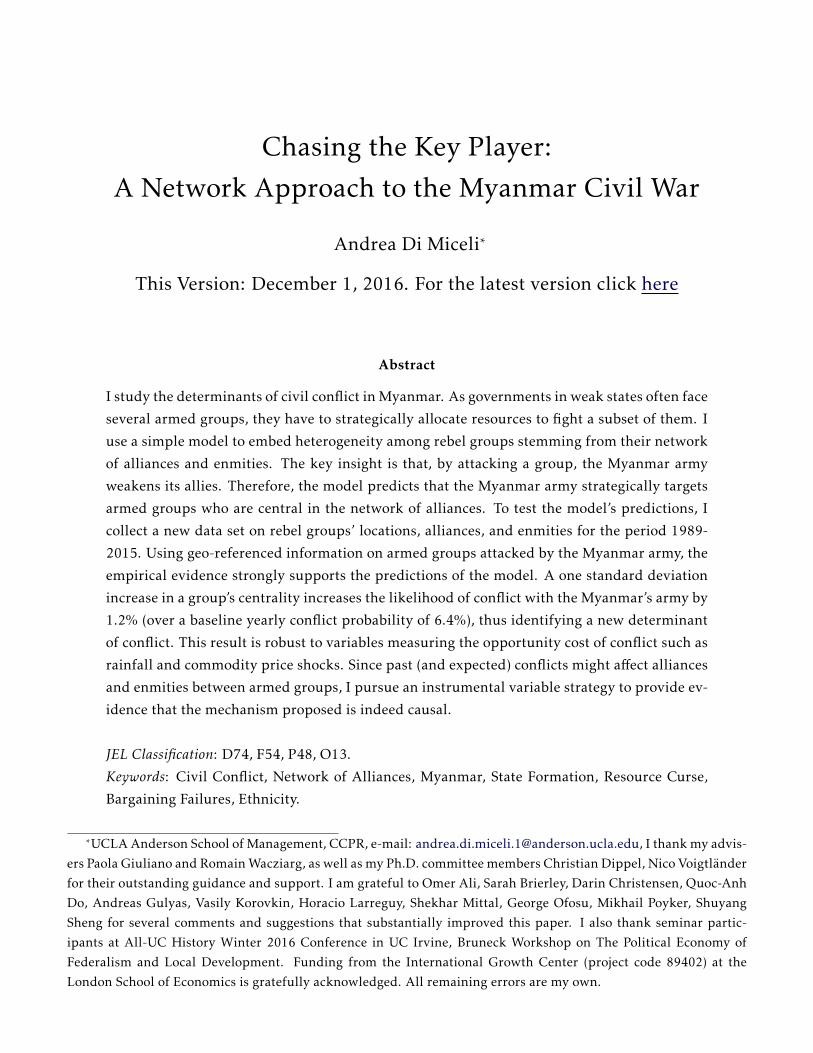
controlled most of the border with China when the mutinies occurred. The network of armed
groups in the country, as well as their alliances and enmities relations, is depicted in Figure 4. A
thin (blue) edge between nodes labels an alliance while a thick (red) edge signals the presence of
an enmity between groups.
In recent years the country adopted a new constitution (2008) and had two parliamentary
elections in 2011 and 2015. The Myanmar army has 25% of the seats reserved in the parliament
so to veto any constitutional reform by the civilian government. Despite the transition, violence
between ethnic armed groups and the Tatmadaw has continued.
11The same anecdote is found in Smith [1999].
9
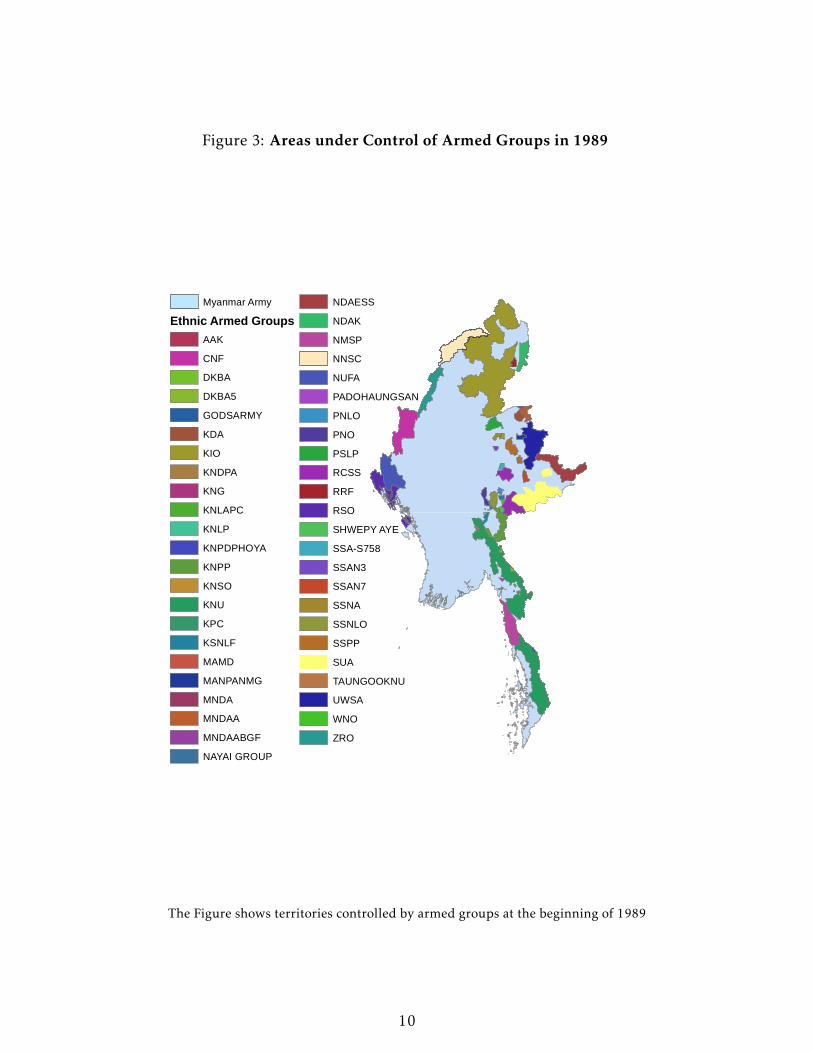
Figure 3: Areas under Control of Armed Groups in 1989
Myanmar ArmyEthnic Armed Groups
AAKCNFDKBADKBA5GODSARMYKDAKIOKNDPAKNGKNLAPCKNLPKNPDPHOYAKNPPKNSOKNUKPCKSNLFMAMDMANPANMGMNDAMNDAAMNDAABGFNAYAI GROUP
NDAESSNDAKNMSPNNSCNUFAPADOHAUNGSANPNLOPNOPSLPRCSSRRFRSOSHWEPY AYESSA-S758SSAN3SSAN7SSNASSNLOSSPPSUATAUNGOOKNUUWSAWNOZRO
The Figure shows territories controlled by armed groups at the beginning of 1989
10

Figure 4: Network of Armed Groups at the end of 1989
Each node represents an armed group. Alliances depicted in thin blue lines, enmities depicted in thick red lines.
11

3 Theoretical Framework
The empirical evidence on the Myanmar conflict shows that, although the Myanmar army faces a
large number of enemies, it only attacks few of them in short time intervals (see Figure 1). In fact,
forty out of the forty-seven armed groups in the sample are involved in at least one violent event
with the Tatmadaw.12 The purpose of the model is to describe how the heterogeneity stemming
from the rich network structure among armed groups explains the Tatmadaw’s decision to attack
each group in a particular time frame.13
The model is divided into two parts: in the first part every armed group chooses its “fighting
capacity” from a linear-quadratic function with externalities. The role of externalities is to keep
track of alliances and enmities over time. In the second step, I assume that the Myanmar army
knows the network structure so that it uses backward induction to reduce the overall fighting
capacity of all armed groups in the network. Reducing the overall fighting capacity of all armed
groups means to eliminate a group from the network. Since armed groups’ fighting capacity
benefits positively from allies (and negatively from enemies) eliminating a group means to reduce
its allies fighting capacity as well. Therefore, the model formalizes the “benefit” of removing an
armed group from the network from the point of view of the Tatmadaw.
The framework draws on the contribution of Ballester et al. [2006] in which there areN agents
that solve a static maximization problem. In what follows I will omit the subscript t because
the problem below is solved in every period independently from what happened in the past (as
well as what will occur in future periods). The environment of the static game is as follows: in
each period every armed group i = 1, ...,n non-cooperatively chooses its fighting capacity xi ≥ 0 to
maximize the following linear-quadratic payoff function:
Ui(x1, ...,xn) = αxi +12ρx2
i +∑j,i
σi,jxixj . (1)
Where α is a linear term set to be equal for every group.14 ρ < 0 is a concavity parameter that
prevents a group from expanding its fighting capacity indefinitely, it also has the intuitive in-
terpretation that the larger a group’s fighting capacity the easier is going to be detectable by the
Tatmadaw (or other enemies). σi,j captures bilateral influences across armed groups: the sign of
σi,j determines whether armed group i is allied with j (σi,j > 0, strategic complements) or an en-
emy (σi,j < 0, strategic substitutes). By the same logic, σi,j = 0 if i and j are neutral. In other words,
12These groups are targeted either directly or through military activity causing casualties in their villages. Restrict-ing the sample to events involving exclusively the Myanmar army and armed groups’ militia confirms the results asshown in Table 10 of the Appendix Section A.6.
13Powell [2012, 2013] shows that heterogeneity in rebels’ characteristics drives the choice of a central governmentthat decides to consolidate power peacefully or through violence. Indeed, rebels can differ along many observable(as well as unobservable) characteristics such as army size, alliances, enmities, territory and resources controlled.
14The model allows for a group specific αi that can accommodate variation at the group level such as resourcewithin the ethnic homeland, army size and population. However, it is much more transparent to control for thesechannels in the empirical analysis and let the model measure exclusively the value of alliances and enmities.
12

the σi,j keep track of the externalities deriving from alliances and enmities between groups.
Ballester et al. [2006] show that, under regularity conditions the above game has a Nash Equi-
librium (their result is replicated in the Appendix Section A.1). Therefore, it is possible to “rank”
armed groups according to their fighting capacity x?i (Σ) where Σ is the x×n matrix including the
σi,j of every armed group. The framework above is ideal to understand the incentives that the
Myanmar army has in attacking a particular armed group. Since the equilibrium level of fighting
capacity is embedded in the network structure of Σ, if the Tatmadaw knows the network struc-
ture it also knows what is the fighting capacity of each armed group. Importantly, this implies that
the Tatmadaw can attack an armed group to reduce the overall fighting capacity in the network.
“Removing” an armed group from the network has two effects: a direct one linked to the removal
of the fighting capacity of group i ( x?i (Σ) ) as well as an indirect one linked to the removal of
the externalities on its allies and enemies σi,j . The intuition for the “indirect effect” is straightfor-
ward: removing a group from the network reduces its allies’ fighting capacity as it reduces their
ability to exchange goods or trade through the group’s territories. The anecdotal evidence of such
channel playing a role between armed groups in Myanmar abounds.15
The Tatmadaw’s problem discussed above is formalized as follows:
Max{∑i x?i (Σ)−
∑i x?i (Σ−i) |i = 1, ...,n}.
Ballester et al. [2006] show that this problem admits a solution that is linked to the contri-
bution of each armed group to the fighting capacity of other armed groups. The intercentrality
parameter ci (Σ) (defined in the Appendix section A.1) captures each armed group contribution
to others ’ fighting capacity.
Theorem 1. (This is Theorem 3 in [Ballester et al., 2006]). Under regularity conditions the key playeri∗ that solves Max {
∑i x?i (Σ) −
∑i x?i (Σ−i) | i = 1, ...,n} is the one that has the highest intercentrality
parameter within the network Σ.
The theorem above sheds light on which armed groups are more likely to be attacked by the
Myanmar army. In particular, it shows that a network statistic, the intercentrality parameter,
carries information on the group’s influence on other armed groups. Therefore, a reduced form
interpretation of Theorem 1 is that armed groups with higher intercentrality parameter (ci (Σ)) are
more likely to be targeted. Anecdotal evidence discussed in section 2 shows that the Tatmadaw
takes into account alliances and enmities in choosing whom to fight.
König et al. [2016] have recently stressed the role of the network of alliances and enmities
during the Congolese civil war. The authors embed the framework of Ballester et al. [2006] to-
gether with a contest success function (Skaperdas [1996]) to show that each group fighting effort
is affected by its alliances and enmities. Differently from their framework, this paper looks at
the effect of alliances and enmities on the probability of being attacked by the Tatmadaw who
15For example, [Lintner, 1999] and [Smith, 1999] document that the CPB was the main weapon supplier to theSSPP during the seventies and eighties. The same authors explain that the SUA was the main buyer of raw opiumfrom smaller armed groups.
13

acts as a rational planner that has full information about the network structure. Moreover, there
is also a conceptual difference between the interpretation of alliances and enmities in the con-
text of this paper and theirs. In the model of König et al. [2016], the fighting effort of an armed
group is decreasing in the number of its first-degree allies and increasing in the number of its
first-degree enemies. This is because armed groups compete for resources, therefore, the more
allies the less competition for resources. By the same token, in their model, fighting increases the
more enemies an armed group has. In my framework, the fighting capacity of a rebel group is
an hypothetical measure of how dangerous that group is to the Myanmar army from a military
perspective. Therefore, the fighting capacity of an armed group is increasing in the number of its
first-degree alliances and reduced in its first-degree enmities.
4 Data
The data is organized at geographical, temporal and armed group level. The unit of observa-
tion is a geographical cell (with side of length 16 miles) observed monthly from January 1989 to
December 2015. In what follows, I describe the sources from which I gathered the data.
4.1 Armed Groups and Network Data for 1989-2015
Data on armed groups’ alliances and enmities come from a variety of sources. The Myanmar con-
flict has been documented by several authors who covered different time frames. In this work I
rely on the following sources to establish the relationships between the forty-seven armed groups
in the sample: i) Lintner [1999, 1990] ii) Smith [1999], for coding alliances until the nineties,
iii) South [2008] and iv) Oo & Min [2007] report alliances for the late nineties until 2006, v) the
Myanmar Peace Center’s website reports alliances and armed groups information with a focus on
the period 2010-2015 vi) information from armed group’s websites vii) Keenan [2013] reports al-
liances and enmities for the period 1989-2013, viii) International Crisis Groups and Euro Burma
Office reports and other papers listed in the Appendix section A.2.
As these sources overlap, a direct comparison between them is possible. There are no conflict-
ing records on whether groups are allied or enemies, i.e. it is never the case that two groups are
reported to be allied in one source and enemies according to another one. However, sometimes
information on small armed groups are only reported by some authors. Following the notation
from the model σi,j summarizes the information coming from the pairwise relationship between
group i and j, this relationship is also referred as dyad in the rest of the paper. If no informa-
tion about alliance (enmity) between armed groups is ever recorded at time t = 1988 the baseline
coding for two groups is neutrality (σi,j = 0). In every period t, alliances (Enmities) are recorded
symmetrically as σi,j = 1 (σi,j = −1).
The number of armed groups is stable over time with the exception of one group being dis-
armed in 1996 (SUA) and two groups entering the network in 1993 (ZRO) and 2010 (AAK). I
14
constructed the network data at the month-year level starting from January 1988 until December
2015. The dataset has a total of 335,295 dyads, alliances make up a total of 16,612 dyads while
there are 6,632 enmities recorded over time. Despite neutrality is the most common dyadic rela-
tionship, the network of armed groups is a giant component (i.e. there is no group that is isolated
from the other armed groups). The network density varies over time from 0.05 and 0.11 so does
its average degree that goes from a minimum of 2.53 to a maximum of 5.11. Variation in these
measures is entirely driven by time variation in the network of alliances and enmities.
4.2 Rainfall Data
Following the influential contribution of Miguel, Satyanath & Sergenti [2004] social scientists
have studied the impact of rainfall (and weather shocks) on inter-group and inter-personal con-
flict. There is a general consensus that abnormal weather variation is associated with violence
(see Burke et al. [2015] for a recent review). The sample of interest in this study is composed
of rural areas in which subsistence agriculture is the norm. It is therefore important to measure
the impact of weather fluctuations on conflict correctly so to purge estimates of the coefficient of
interest from spurious correlations. Even though there are no comprehensive reports on the inci-
dence of subsistence agriculture at the county level, NGOs’ reports suggest that it is the prevalent
activity in rural areas. Rice is the main subsistence crop that is grown in rebels’ areas. Moreover,
in areas whose elevation is too high for rice cultivation, rainfall affects soil moisture throughout
the dry seasons which in turn impacts the yearly opium production. I am not the first to highlight
the causal link between rainfall during the rain season and rice output and how this relationship
affects conflict: Vanden Eynde [2016] shows that Maoist rebels in India are more likely to target
Indian security forces whenever a negative rainfall shock hits a district in which the rebels’ fund-
ing sources are not based exclusively on agricultural income.16
Rainfall data comes from two distinct sources. First, the Global Precipitation Climatology
Centre (GPCC) (Schneider, Becker, Finger, Meyer-Christoffer, Rudolf & Ziese [2011]) covers years
before 2013 and has a spatial resolution of 0.5◦×0.5◦ decimal degrees. Second, the Tropical Rain-
fall Measuring Mission (TRMM) from NASA which covers the period from 1998 onward, is based
on satellite images and has a finer resolution than the GPCC (0.25◦ × 0.25◦ decimal degrees). For
additional details on limitations and advantages of each data source see the discussion in the
Appendix section A.3.
16However, the author also highlights that this effect is reversed whenever agricultural income is the main sourceof funding of Maoist groups.The author argues that the reason for observing variation in the outcome of rainfallshocks on violence depends on the extent to which civilians in Maoist areas have an incentive to cooperate withIndian security forces.
15
4.3 Natural Resources and Price Data
Mapping the location of natural resources in Myanmar is hard because a lot of the mining ac-
tivities occurs without licenses. For this paper, I rely on documents collected by the Extractive
Industries Transparency Initiative (EITI). To date, this is the most complete source of information
on the extractive sector in the country. The coding for mine presence is at the county level. Given
the average size of a county in Myanmar, this choice is similar to Berman, Couttenier, Rohner &
Thoenig [2015] coding of natural resources in Africa. Unfortunately, the EITI report lacks data on
mine discovery. Therefore, there is no temporal variation in mine presence but only geographic
variation in resources. However, temporal variation comes from the international prices of com-
modities available in Myanmar.17
4.4 Generating the Myanmar Grid
The geographical data is organized in cells of size 0.25◦×0.25◦ decimal degrees, these are squares
with side length of 27km (16mi) at the equator. The size of the cells has been chosen in order
to associate armed group presence to each cell. This would have not been possible in the case of
wider cells as the ethnic homelands of multiple groups intersect cells of size 0.5◦×0.5◦. Cells have
both cross-sectional as well as longitudinal differences. Cross-sectional variation includes cell’s
elevation, slope from the Global Agro-Ecological Zones’ database. For every cell administrative
unit classification such as county, district, state and bordering countries, are available from the
Myanmar Information Management Unit. I also collected a cross-sectional measure of the land
use (Land Use UNEP, source year 2000) to know if, within each cell, there are natural resources
in the form of forests. Data on the transportation network in 2010 also comes from the Myanmar
Information Management Unit. An alternative source (DIVA-GIS) reports roads within cells in
1993. Data discussed in the previous sections (4.1, 4.2, 4.3) are thus available at the cell level,
providing time variation in rainfall, value of commodities, armed group presence and conflict
events. Figure 7 in the Appendix Section A.4 shows the cells within Myanmar. There are a total
of 1139 cells within the country but only 600 of them are within territories affected by armed
groups activity between the period of study. These 600 cells are enclosed within 153 counties (the
smallest administrative unit available) and 47 districts. Every cell is observed monthly for twenty-
seven years so that the dataset has nearly two hundred thousand cell-months observations. When
using yearly data the sample has a little more than sixteen thousand observations.
4.5 Conflict Data
Data on conflict outbreaks during years 1989-2015 comes from different sources. The main source
is the Georeferenced Event Dataset (GED) version 3.0 released by the Uppsala Conflict Data Pro-
gram Croicu & Sundberg [2015]. A few caveats of this database need to be discussed. The data
17Additional details on how these were collected in the Appendix section A.5.
16

is organized in dyads so that every event involves only two groups fighting each other. This data
structure can be problematic if fighting activities in the country involve more than two groups. In
order to assess whether this data structure introduces a systematic bias in observing fighting ac-
tors I compared the data from GED with a dataset collected by ACLED for the period 1996-2009
which has a total of 298 events and the advantage of reporting allies in conflict events.18 Only
in 2% of the cases (6 out of the 298 events) an armed group is reported to have an ally on the
battlefield which confirms that alliances are not primarily a means of sharing directly the burden
of fighting on the same battlefield.19
More than 50% of the events in the GED database are recorded as violence against civilians.
As explained in section 2, violence against civilians is an integral part of the Tatmadaw military
strategy to fight rebels’ groups. For this reason, I treat violence against civilians as directed to
the rebel group that occupies the territory in which violence occurs. This choice does not change
estimates’ results nor their interpretation.
Every event in the GED data is coded at the monthly level, this allows the smallest time unit
to be a month. Another advantage of this source is that it records where the event has occurred
within Myanmar reporting the longitude and latitude of each event. This feature allows me to
distinguish between violence against civilians that is unrelated to activity directed against a spe-
cific armed group such as the “Saffron revolution”.20
The second data source of conflict events comes from Myanmar newspapers’ reports and cov-
ers the period from May 2013 to December 2015. The information included in these data is such
that the GED data can be extended until 2015 as fighting sides, events’ date and location are
recorded. The two data sources are aggregated at the monthly and yearly level. Figure 5 shows
the geographical distribution of the events from the two datasets. Once removing events unre-
lated to armed groups the sample consists of 2244 observations, there are a total of forty armed
groups that are attacked at least once by the Tatmadaw. However, some groups are attacked more
frequently than others, the KNU alone makes up for a third of the events in the sample. 40%
of events (897) are classified as violence against civilians while the remainder are coded as vi-
olence between the Tatmadaw and a specific armed group. The dataset used in the empirical
section aggregates, at the cell level, conflict data of Figure 5 as well as the rich cross-sectional and
longitudinal characteristics described in sections 4.1, 4.2, 4.3, 4.4.
18The 298 events only include clashes between armed groups or against civilians, the full dataset reporting riotsand non-violent activities by armed groups has a total of 331 events.
19As discussed in sections 4.1 and 2 alliances are tied to mutual trading interests.20From August to October 2008, Myanmar experienced a series of protests in its major cities that were violently
suppressed by the Myanmar army and local police forces. However, it is well documented that armed groups playedno role in staging or organizing these events. For this reason, in the empirical analysis I drop events coded as violenceagainst civilians that do not occur within armed group’s territories as they cannot be associated with violence targetedtowards a specific armed group. Indeed, all events occurring in areas where the Tatmadaw has the monopoly ofviolence are related to police crackdown on protesters or clashes between Buddhists and Muslims. The unconditionalprobability of violence in these territory is indeed very low (0.2%) when compared with the one in armed groups’territories (1.16%).
17
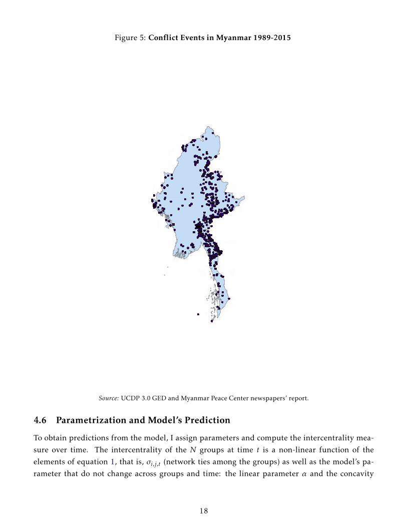
Figure 5: Conflict Events in Myanmar 1989-2015
Source: UCDP 3.0 GED and Myanmar Peace Center newspapers’ report.
4.6 Parametrization and Model’s Prediction
To obtain predictions from the model, I assign parameters and compute the intercentrality mea-
sure over time. The intercentrality of the N groups at time t is a non-linear function of the
elements of equation 1, that is, σi,j,t (network ties among the groups) as well as the model’s pa-
rameter that do not change across groups and time: the linear parameter α and the concavity
18

parameter ρ.21
σi,j,t comes from historical sources (as discussed in section 4.1). Figure 3 shows that the
Myanmar army controls patches of territory virtually everywhere so that moving across different
armed groups’ territory become increasingly difficult as the distance from a group’s homeland
increases.22 Since armed groups’ presence is tied to their ethnic homeland, I weight inter-group
relations by geographic distance. This choice scales down the value of alliances as the distance
between groups increases and is based on the fact that groups far away from each other cannot
trade or help each other on the battlefield. Every, σi,j,t is divided by1
1 +√Disti,j
where Disti,j
is the geodesic distance (in kilometers) between the areas under control of the armed groups.
This choice is similar to Acemoglu, Garcia-Jimeno & Robinson [2015] who estimate ties between
historical Colombian municipalities using geographical distance adjusting for elevation change
among them. To compute these values, I collect and depict maps of armed groups’ presence over
time (Figure 3 is an example for 1989).
Figure 6 shows how the intercentrality parameter changed from 1988 to 2015 for five of the
forty-seven armed groups in the data. From the Figure, it is immediate to see that there is sub-
stantial heterogeneity in intercentrality at the group level. Indeed, while some groups rise and
fall others remain stable over time.
Figure 6: Change in Normalized Intercentrality among five groups (1989-2015)
−2
02
46
Nor
mal
ized
Inte
rcen
tral
ity
1990
m1
1995
m1
2000
m1
2005
m1
2010
m1
2015
m1
Month and Year
KNU UWSA KIOKNPP RCSS
21The intercentrality parameter can be flexibly adjusted to accommodate group specific characteristics through itslinear parameter αi .
22Historical evidence abounds with anecdotes of battalions being wiped out by the Tatmadaw while trying to reachareas controlled by allies (see [Lintner, 1999], [Smith, 1999]).
19

5 OLS Results: Effect of Intercentrality on Conflict
In this section, I test predictions from the stylized model outlined in section 3. I use the rich
cross-sectional and longitudinal variation in the data to identify the role of a group’s intercentral-
ity in explaining the fighting decisions of the Tatmadaw. In sub-sections 5.1 and 5.2, I look at the
impact of commodities shocks and exogenous rainfall fluctuations to show that the coefficient of
interest is robust to the inclusion of other important determinants of civil war. Section 6 discusses
the identification concerns which are addressed through an IV estimation. The dependent vari-
able is a dummy for conflict measured at the cell level. Namely, for each cell c among territories
controlled by armed group i in a given month t, yi,c,t = 1 if conflict is registered within the cell
and zero otherwise.23 While the model predicts which group is more likely to be targeted, the
empirical specification has data for all armed groups regions. The reason for using cells instead
of armed groups as the smallest unit of observation is that, by doing so, it is possible to control
for geographical variation within an armed group’s territory. In fact, armed groups’ territories are
exposed to commodities and weather shocks that are well known to cause conflict in the empiri-
cal literature. For instance, a cell controlled by group i with a gold mine can be attacked because
in period t the international price of gold is high. By the same token, a weather shock can hit
a portion of the territory hosting group i but not the other cells controlled by the same group.
Throughout the paper, I also replicate the main results using armed groups as the units of obser-
vations showing that results are qualitatively unchanged. Equation 2 is the baseline specification
estimated with a Linear Probability Model:
yi,c,t = δ+ β intercentralityi,t +κGeog.Controlsc +χRain Season Droughtc,t +γ Resourcesc+
+ ψ Resources’ Pricest ×Resourcesc +ρyc,t−6 +θt + districtc + εi,c,t. (2)
The baseline specification includes a vector of cell-level geographic controls (labeled Geog.Controlscin the equation above) such as roads, average slope within the cell and a dummy if the cell is be-
tween the border with one of the neighboring countries. Equation 2 also controls for weather
shocks in the form of a dummy called Rain Season Droughtc,t taking value one if the cell experi-
enced a drought during the last rain season. The variable called Resourcesc is a vector of dum-
mies for the presence of natural resources which I interact with a vector of international prices
(Resources’ Pricest ×Resourcesc). θt is a month-year fixed effect. A potential concern stemming
from the stylized model is that it is static, that is, the Myanmar army chooses the group to attack
given the current intercentrality of each group. However, the Tatmadaw observes groups rising
over time and might decide to attack a group that according to the “trend” on the intercentrality
of a particular armed group rather than on its current level. First, if this mechanism is in place,
23The sample excludes territories that are fully under control of the Tatmadaw in which political violence is unre-lated to the ethnic armed groups. Indeed the main form of violence within areas under control of the Tatmadaw isviolence against civilians which is not linked to any of the activities of armed groups in the border areas.
20
then it goes against finding a significant effect on the β coefficient. For instance, if the Myan-
mar army attacks a group because it believes that its future intercentrality is going to increase,
then β̂ is going to be biased downward. Second, I control for the incidence of conflict within
the cell during the previous months. In fact, yc,t−6 in equation 2 denotes a set of dummies for
conflict occurrence within cell c during the last six months. A district fixed effect controls for spe-
cific time-invariant unobservables at the geographic level. Equation 2 does not include an armed
group fixed effect, the reason for this choice is that the cross-sectional variation in armed group’s
intercentrality is essential to understand the Myanmar army’ choice to attack some armed groups
and not others. In fact, if an armed group’s intercentrality is constantly above other groups, the
model predicts that it is more likely to be attacked, regardless of its within group longitudinal
variation. For this reason, identification of the coefficient of interest relies on longitudinal and
cross-sectional variation in armed groups’ intercentrality. Since counties are the smallest admin-
istrative unit for which natural resources’ data is available and their size is roughly equal across
states, I cluster the standard errors at the county level (on average, a county has four cells).24
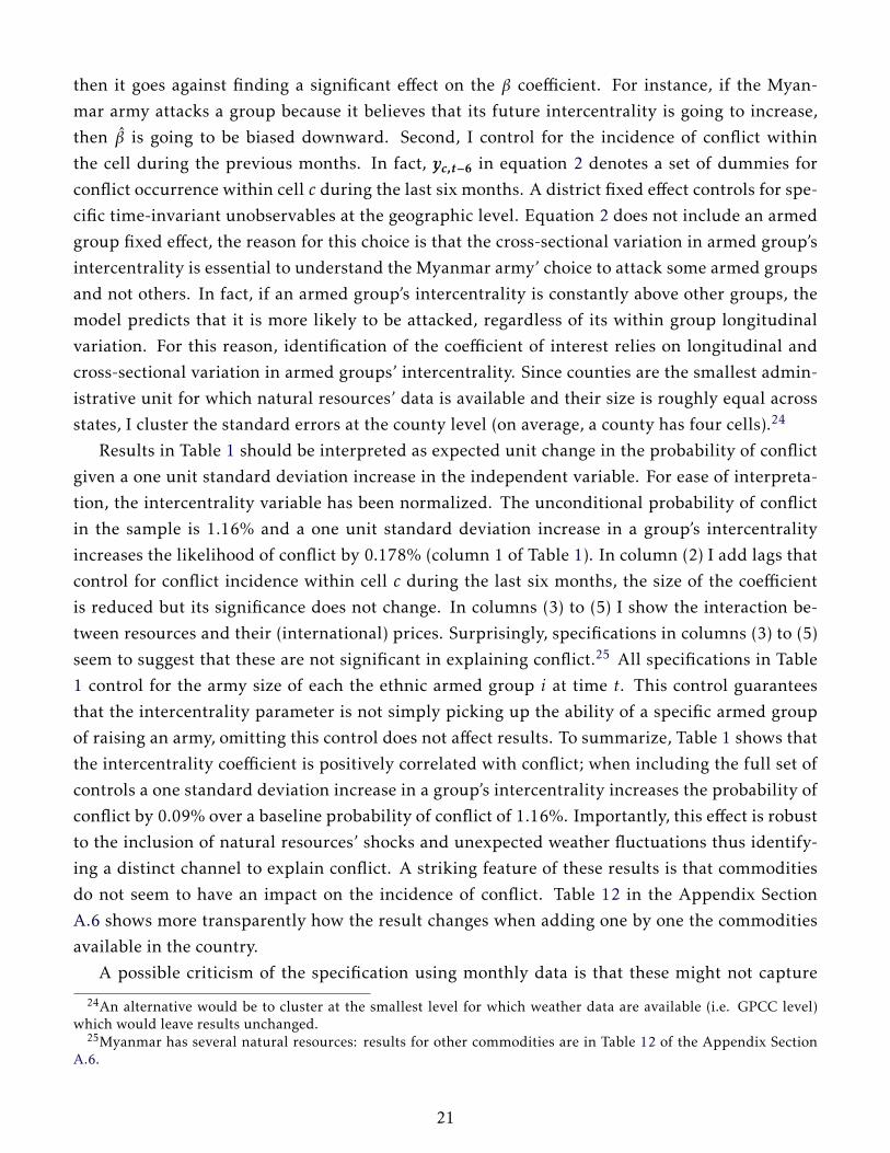
Results in Table 1 should be interpreted as expected unit change in the probability of conflict
given a one unit standard deviation increase in the independent variable. For ease of interpreta-
tion, the intercentrality variable has been normalized. The unconditional probability of conflict
in the sample is 1.16% and a one unit standard deviation increase in a group’s intercentrality
increases the likelihood of conflict by 0.178% (column 1 of Table 1). In column (2) I add lags that
control for conflict incidence within cell c during the last six months, the size of the coefficient
is reduced but its significance does not change. In columns (3) to (5) I show the interaction be-
tween resources and their (international) prices. Surprisingly, specifications in columns (3) to (5)
seem to suggest that these are not significant in explaining conflict.25 All specifications in Table
1 control for the army size of each the ethnic armed group i at time t. This control guarantees
that the intercentrality parameter is not simply picking up the ability of a specific armed group
of raising an army, omitting this control does not affect results. To summarize, Table 1 shows that
the intercentrality coefficient is positively correlated with conflict; when including the full set of
controls a one standard deviation increase in a group’s intercentrality increases the probability of
conflict by 0.09% over a baseline probability of conflict of 1.16%. Importantly, this effect is robust
to the inclusion of natural resources’ shocks and unexpected weather fluctuations thus identify-
ing a distinct channel to explain conflict. A striking feature of these results is that commodities
do not seem to have an impact on the incidence of conflict. Table 12 in the Appendix Section
A.6 shows more transparently how the result changes when adding one by one the commodities
available in the country.
A possible criticism of the specification using monthly data is that these might not capture
24An alternative would be to cluster at the smallest level for which weather data are available (i.e. GPCC level)which would leave results unchanged.
25Myanmar has several natural resources: results for other commodities are in Table 12 of the Appendix SectionA.6.
21
Table 1: Linear Probability Model: Monthly Data
Dependent Variable is Monthly Conflict Dummy
(1) (2) (3) (4) (5)
Intercentrality 0.178** 0.094** 0.094** 0.094** 0.098**(2.006) (2.504) (2.519) (2.523) (2.549)
Rain Season Drought 0.146*** 0.076*** 0.076*** 0.077*** 0.076***(2.894) (2.991) (3.008) (3.004) (2.991)
Army Size -0.010 -0.019 -0.021 -0.016 -0.021(-0.086) (-0.392) (-0.423) (-0.324) (-0.431)
Roads in KM 0.205*** 0.206*** 0.206*** 0.204*** 0.205***(3.757) (3.703) (3.676) (3.653) (3.655)
Lag Conflict 2.315*** 2.315*** 2.315*** 2.315***(14.670) (14.670) (14.670) (14.666)
TeakPr. × TeakForest 0.007 0.008(0.521) (0.543)
Gold Pr. ×Mine -0.030 -0.027(-1.034) (-0.936)
# Observations 195,641 195,641 195,641 195,641 195,641# Clusters 153 153 153 153 153Adj. R-Sq. 0.026 0.169 0.169 0.169 0.169Month F.E. × Year F.E. Yes Yes Yes Yes YesDistrict F.E. Yes Yes Yes Yes Yes
Coefficients from Linear Probability Model show the expected percent change in conflictprobability with a one standard deviation change in the indep. variable. The baseline prob-ability of conflict in a month is 1.16%. T-statistic in parentheses from S.E. clustered at thetownship level (153 clusters). Estimation period: monthly data from Jan 1989 to Dec. 2015.Controls include Fixed Effects for District, Month-Year, cell average slope, border dummy, in-teraction of international prices of commodities and dummies for their presence at the countylevel. Columns 2 to 5 include six dummies for lagged conflict within the cell in the previousmonths. * p<.1, ** p< .05, *** p< .01
the effect of a price increase on conflict. Indeed, several studies in the literature use yearly data
when studying the effect of exogenous price shocks on conflict ([Berman et al., 2015], [Dube &
Vargas, 2013]). To address this issue, I estimate equation 2 using yearly data where the baseline
probability of conflict is 6.4%. Results are in Table 2: a one standard deviation increase in group
i’s intercentrality is associated with an expected increase in the probability of conflict by 1.2
percentage points (occurring in any cell controlled by the group). When switching from monthly
to yearly data interactions between prices and resources are significant only for Teak. Yearly data
fail to capture the effect of a drought in the previous rain season, this is because the rain season
ends in August and consequences of droughts are likely to spill over on different calendar years
(I discuss this issue more in detail in subsection 5.2). Overall, Tables 1 and 2 show that a group’s
alliances and enmities have a sizable impact on the probability of conflict. The magnitude of
the intercentrality coefficient is greater than the effect of exogenous weather and commodities’
shocks.
22

Table 2: Linear Probability Model: Yearly Data
Dependent Variable: Yearly Conflict Dummy
(1) (2) (3) (4) (5)
Intercentrality 1.242*** 1.224*** 1.221*** 1.234*** 1.234***(2.903) (3.236) (3.228) (3.268) (3.239)
Rain Season Drought 0.259 0.246 0.235 0.249 0.231(1.216) (1.267) (1.231) (1.273) (1.205)
Army Size -0.136 -0.154 -0.130 -0.096 -0.055(-0.234) (-0.297) (-0.255) (-0.186) (-0.106)
Roads in KM 2.288*** 2.015*** 2.019*** 1.983*** 1.974***(4.104) (4.028) (4.001) (3.940) (3.903)
Lag Conflict 4.315 *** 4.310*** 4.310*** 4.294***(10.673) (10.653) (10.611) (10.581)
TeakPr. × TeakForest 0.471*** 0.507***(3.009) (3.283)
Gold Pr. ×Mine -0.181 -0.167(-0.808) (-0.742)
# Observations 16940 16940 16940 16940 16940# Clusters 153 153 153 153 153Adj. R-Sq. 0.084 0.120 0.120 0.121 0.121Year F.E. Yes Yes Yes Yes YesDistrict F.E. Yes Yes Yes Yes Yes
Coefficients from Linear Probability Model show the expected percent change in conflictprobability with a one standard deviation change in the indep. variable. The baseline prob-ability of conflict in a year is 6.39%. T-statistic in parentheses from S.E. clustered at thetownship level (153 clusters). Estimation period: yearly data from Jan 1989 to Dec. 2015.Controls include Fixed Effects for District and Year, cell average slope, border dummy, inter-action of international prices of commodities and dummies for their presence at the countylevel. Columns 2 to 5 include a dummy for lagged conflict within the cell in the previous year.* p<.1, ** p< .05, *** p< .01
Additional robustness tests are shown in the Appendix Section A.6. In Table 10, I show re-
sults of running the baseline specification of column (5) (in Tables 1 and 2) using armed groups
observed monthly (yearly in columns (2-3)) as unit of observations. That is, the dependent vari-
able becomes yi,t = 1 if group i is attacked in t and zero otherwise. Doing so confirms that a
group’s intercentrality is positively correlated with the likelihood of being attacked by the Tat-
madaw. Moreover, this specification clusters the Standard Errors at the rebel group level showing
robustness to alternative cluster definitions. In Table 11, I drop events coded as violence against
civilians in armed groups’ territories. Hence, the coefficient of interest in Table 11 is estimated
exclusively using conflict between the Tatmadaw and ethnic armed groups. Doing so increases
the precision with whom the coefficient of interest is estimated. In Table 12, I show the effect of
each commodity’s price increase on conflict. I first add them one by one, and then have them all
together when estimating equation 2. Additional robustness checks in which I analyze how the
precision of the estimates varies for different cluster definition in Section 6.1. The next section
23

shows that the coefficient of interest is robust to the inclusion of different methods to measure the
effect of commodities’ shocks on conflict.
5.1 Commodities and Conflict in Myanmar
Several seminal papers have shown the effect of natural resources on interstate and intra-state
conflict.26 In this study, I focus on a high spatial resolution data to measure the effect of com-
modities on conflict. Columns (3)-(5) in Tables 1 and 2 show that some commodities have an
impact on conflict. A criticism of this approach is that conflict need not be observed within the
cell in which the commodity whose value suddenly increased is present. That is, conflict might
spill over nearby cells, and the coding above is not capturing the true effect of shocks to commodi-
ties.27 To address this concern, I build a measure of resources at the ethnic homeland level for
each group. Namely, for each armed group I compute the variable Ethnic Homeland Resourcei =∑kMinek1(Ethnic Homelandi) where Minek is a dummy that equals one if commodity k is avail-
able in the groups’ ethnic homeland. I normalized prices of commodities so that I could have
a single price index capturing the effect of the overall market fluctuation at time t: pt =∑k pt,k,
(with pt,k being the price of commodity k in t). Therefore, the interaction term is computed as
the sum of interactions: P riceIndex × EthnicHomelandResources =∑k pk ×Minek. The equation
to estimate becomes the following:
yi,c,t = δ+ β intercentralityi,t +θt +ρyc,t−6 + γ Ethnic Homeland Resourcesi+
+ ψ Price Indext ×Ethnic Homeland Resourcesi + κGeog.Controlsc +
+ χRain Season Droughtc,t + districti + εi,c,t (3)
Table 3 shows results of this exercise when using monthly (column (1)) and yearly (column
(3)) data.28 Controlling for group specific shocks does not change the significance of the coeffi-
cient estimating the effect of intercentrality on conflict. Columns (1) and (3) show that shocks to
commodities are positively correlated with conflict, a one standard deviation increase in the inter-
action of prices and resources increases the probability of monthly (annual) conflict by 0.2 (2.4)
percentage points. Results in Table 3 also show that the total resources in a group’s homeland do
not mechanically cause a group to be central as the coefficient on the variable Ethnic HomelandResources is not significantly different from zero. Indeed, adding the variable measuring resources
at the ethnic homeland does not change the significance nor the magnitude of the intercentral-
ity coefficient in Table 3 when compared to Table 1 and 2. This result is important as it shows
that the positive correlation between intercentrality and conflict is not capturing a spurious cor-
26Among them [Caselli, Morelli & Rohner, 2015], [Dube & Vargas, 2013], [Berman et al., 2015], [Michalopoulos &Papaioannou, 2016].
27Note that this concern is mitigated by the coding of resources’ presence. Whenever a county has a resource, allcells within the county are coded to have that resource.
28The month-year fixed effect θt picks up the effect of P riceIndex which is omitted from equation 3.
24

relation with a group’s resources but identifying a channel that is salient for establishing which
armed group the Myanmar army should attack. In columns (2) and (4) of Table 3, I interact a
group’s intercentrality with the shock that the group receives to the value of its resources. Since
the intercentrality parameter has been normalized, it takes both positive and negative values.
Hence, commodities shocks are (exogenous) “shifters” that should matter more to groups with
higher intercentrality. Coefficients in columns (2) and (4) confirm this conjecture.
Table 3: Commodities’ Shocks to Intercentrality
Estimates from Linear Probability Model
Dependent Variable: Monthly Conflict Dummy Yearly Conflict Dummy(1) (2) (3) (4)
Intercentrality 0.125*** 0.149*** 1.249*** 1.206***(2.992) (3.298) (3.109) (2.757)
Intercentr.× Pr. Index × Ethnic Hom. Res. 0.199*** 1.002***(3.826) (2.573)
Price Index × Ethnic Homeland Resources 0.193** 2.443***(2.236) (4.649)
Ethnic Homeland Resources 0.090 0.098 0.971 1.181(1.032) (1.089) (1.129) (1.323)
# Observations 195,641 195,641 16,940 16,940# Clusters 153 153 153 153Adj. R-Sq. 0.139 0.139 0.124 0.122Month F.E. × Year F.E. Yes Yes No NoYear F.E. No No Yes YesDistrict F.E. Yes Yes Yes Yes
Coefficients from Linear Probability Model show the expected percent change in conflict probability with a one stan-dard deviation change in the indep. variable. The baseline probability of conflict in a year (month) is 6.39% (1.16%).T-statistic in parentheses from S.E. clustered at the township level (153 clusters). Estimation period: monthly datafrom Jan 1989 to Dec. 2015. in columns (1)-(2), Yearly data in (3)-(4). Controls in every regression include Fixed Effectsfor District, Indicator for below average rainfall during the previous rain season, cell average slope, border dummy.Columns (1) and (3) include six dummies for lagged conflict within the cell in the previous months. Columns (2) and(4) include a dummy for conflict within the cell in the previous year. * p<.1, ** p< .05, *** p< .01
5.2 Rainfall and Conflict in Myanmar
The goal of this section is to discuss how the variable measuring droughts during the rainy season
is constructed and to show that results are robust to alternative definitions of drought and sources
measuring rainfall in Myanmar.
I measure negative deviations from long-run cell averages with a dummy that equals one
whenever the total rainfall in the rain season is in the lowest quartile of the distribution of histori-
cal rainfall within each cell during the rain season. I use this information to create the Rain SeasonDrought variable which takes value one from the end of the rain season until the beginning of the
next rain season. I do this because rainfall shocks can have a delayed effect on conflict (something
25

emphasized by Burke et al. [2015] in their review).
Table 4 shows estimates from a linear probability model with monthly data and the full set of
controls in equation 2. What changes in this Table is the way the Drought variable is constructed.
Columns (1) and (3) look at abnormal deviations occurred throughout the full rain season span
using the two distinct sources (TRMM and GPCC) of rainfall data. Using the TRMM data, the
effect of a drought is positively correlated with conflict and significant at the 10% level, but this
effect vanishes with the GPCC data. In columns (2) and (4) I focus on the last two months of the
rain season: doing so shows that both sources capture a positive correlation between droughts
and conflict. Note that the effect of a drought during the rain season is below eighty percent of
the effect of a one standard deviation in a group’s intercentrality.
Table 4: LPM estimates: Rainfall and Conflict
Dependent Variable: Monthly Conflict Dummy
(1) (2) (3) (4) (5)
Intercentrality 0.095** 0.098** 0.095** 0.097** 0.095**(2.472) (2.504) (2.576) (2.547) (2.479)
Rain Season Drought (TRMM) 0.046*(1.655)
Rain Season Drought, last 2 months (TRMM) 0.076***(2.991)
Rain Season Drought (GPCC) -0.046(-0.747)
Rain Season Drought, last 2 months (GPCC) 0.067**(2.296)
Negative Deviation 0.076**(2.272)
Positive Deviation 0.065**(2.404)
# Observations 195,641 195,641 195,641 195,641 195,641# Clusters 153 153 153 153 153Adj. R-Sq. 0.167 0.169 0.169 0.169 0.170Month F.E. × Year F.E. Yes Yes Yes Yes YesDistrict F.E. Yes Yes Yes Yes Yes
Coefficients from Linear Probability Model show the expected percent change in conflict probability with a one stan-dard deviation change in the indep. variable. The baseline probability of conflict in a month is 1.16%. T-statistic inparentheses from S.E. clustered at the township level (153 clusters). Estimation period: monthly data from Jan 1989 toDec. 2015. Controls include Fixed Effects for District, Month-Year, cell average slope, border dummy, six dummies forlagged conflict within the cell in the previous months interaction of international prices of commodities and dummiesfor their presence at the county level. * p<.1, ** p< .05, *** p< .01
The last column studies the presence of non-linear responses to weather shocks as found in
previous studies in the literature (Hidalgo, Naidu, Nichter & Richardson [2010]). Simply, too
much rain can also damage harvests causing negative income shocks to local population or armies
relying on them for food and taxes. To show robustness of the intercentrality coefficient to non-
26

linear responses of weather shocks, I construct a dummy called Negative Rainfall Deviation (Pos-itive Rainfall Deviation) taking value one whenever the monthly deviation from average rainfall
is 98% below (above) the long run monthly average. The inclusion of these events does not af-
fect the intercentrality coefficient’s significance. In conclusion, regardless of the source used, the
coefficient of interest is not affected by deviation from average rainfall in the country.
6 Instrumental Variables Estimation
The evidence presented so far highlights a positive correlation between how connected a group
is and the probability of being attacked by the Myanmar army. These results are robust to the
inclusion of controls motivated by the literature studying civil wars. However, the above results
might still be affected by identification problems which I discuss below.
The intercentrality of a particular armed group can react to expected threats of conflict with
the Tatmadaw. That is, some groups form alliances with each other because they expect to be
attacked in the short term. While the literature on the civil war in Myanmar does not provide
direct evidence on this issue, the concern of reverse causality between conflict and Intercentrality
is legitimate. Moreover, this criticism can work in the opposite direction: groups can break al-
liances to avoid conflict with the Tatmadaw. Therefore, alliances and conflict can be, at the same
time, outcomes and explanatory variables of a simultaneous equation model. Failing to account
for the true equation that determines the interplay of alliances and conflict causes an omitted
variables bias in the estimates above. An additional concern is that the intercentrality variable is
capturing a spurious correlation with conflict caused by time-varying unobservables at the armed
group level. I address these concerns through an instrumental variables estimation.
The intercentrality parameter ci,t(Σt) is a non-linear function of the network structure de-
scribed by the matrix Σt. As the variable of interest is based on the (potentially) endogenous
network structure observed at time t, the very first step for an instrumental variable is to predict
a counterfactual network of alliances and enmities. The counterfactual network structure is then
used to compute the intercentrality parameter which is an instrument for the endogenous one
(used in previous regressions). Since the instrument is a non-linear function of the counterfac-
tual network, concerns on whether variables impacting the (counterfactual) network formation
are excludable from a regression on conflict are addressed by including them in the instrumental
variable estimation. To predict the network, I apply standard assumptions in the literature study-
ing how dyadic (i.e. inter-groups) relationships are formed and use these to estimate parameters
that drive cross-sectional and longitudinal variation in the (predicted) network structure.
I estimate a choice model of link formation to predict the pairwise relationships, i.e. the σi,j,t,
that are the entries of the adjacency matrix of alliances and enmities Σt. Namely, I estimate
parameters of the empirical link formation model of equation (4) by maximum likelihood as a
standard multinomial logit estimator. Ui,j,t(σ ) (where σ ∈ {−1,0,1}) is the dyad’s joint utility from
27

forming a positive (negative or neutral) link. This formulation assumes that utility is transferable
across directly linked agents and that the observed connection is the one that maximizes the two
groups’ utility.
Ui,j,t(σ ) = FEi +FEj + δLing.Disti,j + βGeog.Disti,j + γ pt +
+ κ CommonResourcesi,j + χ pt CommonResourcesi,j +ui,j,t. (4)
The observable and unobservable components that affect the choice are discussed below:
1. FEi ,FEj . The presence of groups’ fixed effects is based on models of network formation
that leave each group’s degree heterogeneity unrestricted.29 As shown by Graham [2015]
for a link formation rule similar to the one above, omitting the groups’ fixed effects from (4)
causes the estimates for β, δ, γ , χ, κ to be biased. A standard feature of networks is that
nodes vary in the general surplus they generate when forming a link. Therefore, including
fixed effects also takes into account that some groups are better than others at establishing
alliances (or enmities). For example, the RSO and NSCN-K only have one connection (i.e.
degree one) with other armed groups but the KNU, RCSS and KNPP always have degrees
that are above the average in the network.30
2. Linguistic Distancei,j , Geographic Distancei,j are pre-determined pairwise variables that
capture homophily stemming from observable characteristics, respectively, linguistic prox-
imity between armed groups and geographic distance of groups i and j’s ethnic home-
lands.31 The inclusion of linguistic distance is justified on the grounds of the literature
studying ethnicity and conflict. For instance, Spolaore & Wacziarg [2016] find that genet-
ically similar populations are more likely to engage in inter-state conflict. Other authors
Esteban et al. [2012] point out that ethnic polarization increases the risk of civil conflict.
The distance between ethnic homelands proxies for the likelihood that two groups interact
with each other. The rationale is that the further away two groups are from each other the
less they will benefit from a connection.
3. κ CommonResourcesi,j + γ pt + χ pt CommonResourcesi,j : these variables report the in-
teractions between the monthly international prices of commodities at time t and a series
of dummies (CommonResourcesi,j) for the resources shared between groups. To be more
specific, CommonResourcesi,j is a matrix that includes a dummy for every resource that is
shared by at least two different armed groups. The dummy equals one whenever groups
i and j share a particular resource and zero otherwise. Their inclusion is motivated by the
29See Graham [2014b] for an introduction to empirical models of network formation.30This feature is common among all type of networks observed in nature (friends in school, trading partners, etc.)
in which some nodes act as hubs while others have fewer connections.31Linguistic distance is a measure of how close two languages are given their shared nodes in the linguistic tree.
Desmet, Ortuño-Ortín & Wacziarg [2012] introduced this measure.
28

influential contribution of Caselli et al. [2015] who show that the presence of resources close
to the border between two countries makes conflict between them more likely. Even though
conflict between armed groups is rare in Myanmar, resources play an important role for
groups’ relationships. For example, South [2008] when commenting an agreement between
KIO, RRF and NDA-K in 2005 writes that: “The formal reconciliation of KIO, RRF and
NDA-K territorial disputes (...) seems to have been agreed primarily in order to facilitate
logging activities in the rich forests of Northeast Kachin State rather than due to any great
revival of fraternal spirit.” Other anecdotes stress how opium growing groups have to rely
on groups specializing in trading opium to sell and refine their opium harvests. I argue that
the exogenous variation in the price of shared commodities drives the armed groups’ incen-
tives to meet and discuss how to share them (or how to smuggle across the border without
the Tatmadaw). Importantly, shared resources differ from the Ethnic Homeland Resources of
Table 3, as these are only resources shared among ethnic groups and not representative of
the overall resources within a group’s ethnic homeland.32 Moreover, since the instrument is
a non-linear function of the predicted network, I will control transparently for the effect of
resources in the two-stage least squares estimation.
4. ui,j,t are idiosyncratic components assumed to be i.i.d across dyads, the distributional as-
sumption on them (type I extreme-value) ensures that we can write the conditional log-
likelihood and estimate parameters through a multinomial logit specification.
A limitation of this modeling choice is that it rules out interdependent link preferences. For
example, consider three armed groups i, j and k, the decision of i and j to form an alliance is
(assumed to be) independent from the potential alliance (or enmity) between i and k as well as j
and k.33
Estimating equation (4) poses the well-known incidental parameter problem Neyman & Scott
[1948]: parameters’ estimates are biased because of the estimation error generated by the fixed
effects. Unfortunately, there is no formal result in the econometric theory that quantifies the bias
deriving from estimating the above model.34 Since the number of observations, N (N−1)2 , grows
faster than the number of parameters to estimate,N , and the time series is very long (324 months),
I choose not to correct for the (formally unknown) bias deriving from estimating fixed effects in a
non-linear model.
32For instance, whenever a group has the “monopoly” over a certain resource this will not enter the CommonResource matrix.
33I am not the first that uses this assumption to predict alliances between groups: Lai & Reiter [2000] use it topredict alliances between nations from 1816 until 1992.
34Graham [2015] solves a similar problem for a simpler Joint Maximum Likelihood as in his empirical modelgroups are either connected or not. To see how this problem differs from Hahn & Newey [2004], note that for eacharmed group I observe N − 1 choices in every t. In fact, the number of fixed effects to estimate, N , is an order ofmagnitude smaller than the number of observations in the data as every period N (N−1)
2 observations constitute thesample size through which the F.E. is estimated.
29
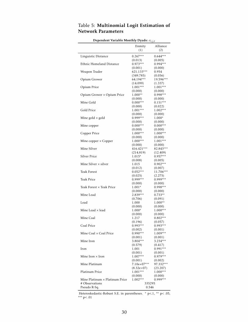
Table 5: Multinomial Logit Estimation ofNetwork Parameters
Dependent Variable Monthly Dyads: σi,j,t
Enmity Alliance(1) (2)
Linguistic Distance 0.267*** 0.644***(0.013) (0.005)
Ethnic Homeland Distance 0.973*** 0.994***(0.001) (0.000)
Weapon Trader 621.133*** 0.954(349.785) (0.056)
Opium Grower 64.194*** 19.596***(14.099) (1.337)
Opium Price 1.001*** 1.001***(0.000) (0.000)
Opium Grower × Opium Price 1.000** 0.998***(0.000) (0.000)
Mine Gold 0.000*** 0.151***(0.000) (0.022)
Gold Price 1.001*** 1.002***(0.000) (0.000)
Mine gold × gold 0.999*** 1.000*(0.000) (0.000)
Mine copper 0.000*** 0.000***(0.000) (0.000)
Copper Price 1.000*** 1.000***(0.000) (0.000)
Mine copper × Copper 1.000*** 1.001***(0.000) (0.000)
Mine Silver 416.421*** 82.843***(214.819) (12.409)
Silver Price 1.015* 0.957***(0.008) (0.005)
Mine Silver × silver 1.015 0.902***(0.012) (0.007)
Teak Forest 0.052*** 11.706***(0.025) (2.275)
Teak Price 0.999*** 0.999***(0.000) (0.000)
Teak Forest × Teak Price 1.001* 0.998***(0.000) (0.000)
Mine Lead 2.839*** 0.733**(0.706) (0.091)
Lead 1.000 1.000**(0.000) (0.000)
Mine Lead × lead 1.000* 1.000***(0.000) (0.000)
Mine Coal 1.217 0.802***(0.196) (0.057)
Coal Price 0.993*** 0.993***(0.002) (0.001)
Mine Coal × Coal Price 0.990*** 1.009***(0.001) (0.001)
Mine Iron 3.804*** 3.234***(0.579) (0.417)
Iron 1.001 0.991***(0.001) (0.001)
Mine Iron × Iron 1.007*** 0.979***(0.001) (0.002)
Mine Platinum 7.10e+07*** 97.332***(8.32e+07) (23.207)
Platinum Price 1.001*** 1.000***(0.000) (0.000)
Mine Platinum × Platinum Price 1.002*** 0.999***# Observations 335295Pseudo R-Sq. 0.546
Heteroskedastic-Robust S.E. in parentheses. * p<.1, ** p< .05,*** p< .01
30

Results from the multinomial logit estimation are in Table 5 in which Relative Risk Ratios are
expressed over the base outcome (neutrality). For example, the relative risk ratio of being ene-
mies over being neutral for a one-unit increase in Linguistic Distance between i and j is expected
to decrease by a factor of 0.267 (holding the other variables fixed). This result implies that as
Linguistic Distance increases between groups their likelihood of being enemies in the network
decreases. Note that the interaction between pt ×Common Resourcesi,j are significant and help
to explain what time variation generates alliances and enmities between groups. In Table 12 (Ap-
pendix Section A.6), I show that most of these variables do not seem to have a direct effect on the
probability of conflict.
Table 6: Instrumental Variable Estimation
Dependent Variable Monthly Conflict Dummy
OLS Red.Form 2SLS First Stage(1) (2) (3) (4)
Intercentrality 0.091** 0.103**(2.432) (1.961)
Instrum. Intercentrality 0.079** 0.768***(2.014) (13.410)
# Observations 195,641 195,641 195,641 195,641# Clusters 153 153 153 153Adj. R-Sq. 0.169 0.169 0.169 0.482F-test 179.8Partial R-sq. 0.30Year F.E. ×Month F.E. Yes Yes Yes YesDistrict F.E. Yes Yes Yes Yes
Coefficients from Linear Probability Model show the expected percent change in con-flict probability with a one standard deviation change in the indep. variable in columns(1)-(3), column (4) reports unstandardized regression coefficients. The baseline prob-ability of conflict in a month is 1.16%. T-statistic in parentheses from S.E. clustered atthe township level (153 clusters). Estimation period: monthly data from Jan 1989 toDec. 2015. Controls include KM of Roads within the cell, altitude, dummy for droughtduring the last two months of the rain season, international prices of commodities aswell as dummies for their presence at the county level. * p<.1, ** p< .05, *** p< .01.
Table 6 reports results from the instrumental variable estimation when the baseline equation
in column (6) of Table 1 is estimated through a 2SLS procedure. The coefficient on the IV is
slightly larger than the OLS one: a one standard deviation increase in a group’s intercentrality in-
creases the expected probability that the Tatmadaw attacks a cell controlled by the group by 0.11
percentage points (as opposed to 0.09 in the OLS). The first stage diagnostics for the IV are shown
in column (4): the correlation between the instrumented intercentrality and the “endogenous”one
is high and precisely estimated as shown by the Partial R-squared (0.30) and F-test (180.22). Re-
sults with yearly data as well as using armed groups as units of observations are in Table 14 and
15 in the Appendix section A.7. These alternative specification bolster the result obtained with
31

monthly data.35 An interpretation for why the IV coefficient is larger than the OLS one is that
the Tatmadaw attacks groups before they achieve their “full” network potential in terms of allies.
That is, armed groups are attacked when their influence on the network is rising but has not yet
reached the highest intercentrality that each group can potentially achieve. Note that this pat-
tern is consistent with a rational model explaining war as the outcome of shifting distribution of
power between groups ([Fearon, 1995], [Powell, 2012]) as well as with models of preventive wars
[Jackson & Morelli, 2011]. Once the Tatmadaw realizes that the “power” of one group is growing
rapidly (through alliances) war becomes the first-best choice to avoid the future shift in the power
distribution.
Table 7: IV Estimation without Fixed Effects to Predict the σi,j,t
Dependent Variable Monthly Conflict Dummy
OLS Red.Form 2SLS First Stage(1) (2) (3) (4)
Intercentrality 0.091** 0.736***(2.432) (4.889)
Instrum. Intercentrality 0.237*** 0.323***(4.529) (5.941)
# Observations 195,641 195,641 195,641 195,641# Clusters 153 153 153 153Adj. R-Sq. 0.169 0.169 0.169 0.482F-test 35.29Partial R-sq. 0.04Year F.E. ×Month F.E. Yes Yes Yes YesDistrict F.E. Yes Yes Yes Yes
Coefficients from Linear Probability Model show the expected percent change in con-flict probability with a one standard deviation change in the indep. variable in columns(1)-(2), column (3) reports unstandardized regression coefficients. The baseline proba-bility of conflict in a month is 1.16%. T-statistic in parentheses from S.E. clustered atthe township level (153 clusters). Estimation period: monthly data from Jan 1989 toDec. 2015. Controls include KM of Roads within the cell, altitude, dummy for droughtduring the last two months of the rain season, international prices of commodities aswell as dummies for their presence at the county level. * p<.1, ** p< .05, *** p< .01.
The instrumental variable results follow even excluding the fixed effects coefficients from the
predictions of σi,j,t after estimating (4). That is, I use the armed groups’ Fixed Effects to esti-
mate equation (4) so that the remaining parameters (δ ,β ,γ ,κ ,χ ) are correctly estimated but I
omit their parameters’ estimates when predicting σi,j,t. Doing so guarantees that the unobserved
group-specific heterogeneity is exclusively used to correctly estimate the remaining parameters
and not to predict the network structure.36 Results from this exercise are shown in Table 7 (results
for yearly data are in Table 16 in Appendix Section A.7). Even though the predicted intercentral-
35Estimates’ precision in both monthly and yearly data is increased if events coded as violence against civilians areexcluded from the sample (results available upon request).
36I thank Quoc-Anh Do, Horacio Larreguy and Nico Voigtländer for discussions and suggestions on this issue.
32
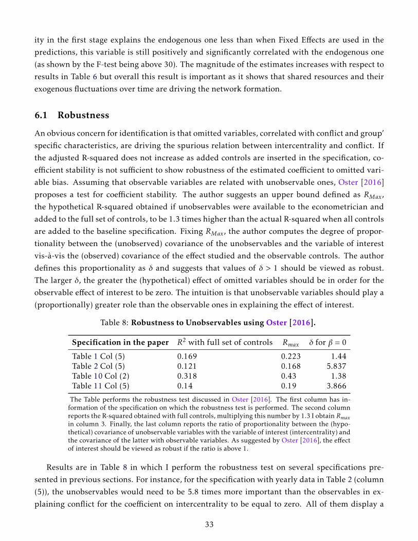
ity in the first stage explains the endogenous one less than when Fixed Effects are used in the
predictions, this variable is still positively and significantly correlated with the endogenous one
(as shown by the F-test being above 30). The magnitude of the estimates increases with respect to
results in Table 6 but overall this result is important as it shows that shared resources and their
exogenous fluctuations over time are driving the network formation.
6.1 Robustness
An obvious concern for identification is that omitted variables, correlated with conflict and group’
specific characteristics, are driving the spurious relation between intercentrality and conflict. If
the adjusted R-squared does not increase as added controls are inserted in the specification, co-
efficient stability is not sufficient to show robustness of the estimated coefficient to omitted vari-
able bias. Assuming that observable variables are related with unobservable ones, Oster [2016]
proposes a test for coefficient stability. The author suggests an upper bound defined as RMax,
the hypothetical R-squared obtained if unobservables were available to the econometrician and
added to the full set of controls, to be 1.3 times higher than the actual R-squared when all controls
are added to the baseline specification. Fixing RMax, the author computes the degree of propor-
tionality between the (unobserved) covariance of the unobservables and the variable of interest
vis-à-vis the (observed) covariance of the effect studied and the observable controls. The author
defines this proportionality as δ and suggests that values of δ > 1 should be viewed as robust.
The larger δ, the greater the (hypothetical) effect of omitted variables should be in order for the
observable effect of interest to be zero. The intuition is that unobservable variables should play a
(proportionally) greater role than the observable ones in explaining the effect of interest.
Table 8: Robustness to Unobservables using Oster [2016].
Specification in the paper R2 with full set of controls Rmax δ for β = 0
Table 1 Col (5) 0.169 0.223 1.44Table 2 Col (5) 0.121 0.168 5.837Table 10 Col (2) 0.318 0.43 1.38Table 11 Col (5) 0.14 0.19 3.866
The Table performs the robustness test discussed in Oster [2016]. The first column has in-formation of the specification on which the robustness test is performed. The second columnreports the R-squared obtained with full controls, multiplying this number by 1.3 I obtain Rmaxin column 3. Finally, the last column reports the ratio of proportionality between the (hypo-thetical) covariance of unobservable variables with the variable of interest (intercentrality) andthe covariance of the latter with observable variables. As suggested by Oster [2016], the effectof interest should be viewed as robust if the ratio is above 1.
Results are in Table 8 in which I perform the robustness test on several specifications pre-
sented in previous sections. For instance, for the specification with yearly data in Table 2 (column
(5)), the unobservables would need to be 5.8 times more important than the observables in ex-
plaining conflict for the coefficient on intercentrality to be equal to zero. All of them display a
33
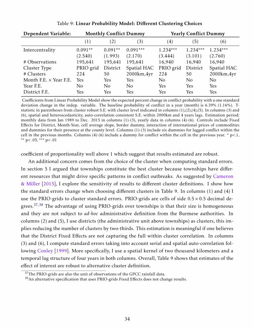
Table 9: Linear Probability Model: Different Clustering Choices
Dependent Variable: Monthly Conflict Dummy Yearly Conflict Dummy
(1) (2) (3) (4) (5) (6)
Intercentrality 0.091** 0.091** 0.091*** 1.234*** 1.234*** 1.234***(2.540) (1.993) (2.170) (3.444) (3.101) (2.760)
# Observations 195,641 195,641 195,641 16,940 16,940 16,940Cluster Type PRIO grid District Spatial HAC PRIO grid District Spatial HAC# Clusters 224 50 2000km,4yr 224 50 2000km,4yrMonth F.E. × Year F.E. Yes Yes Yes No No NoYear F.E. No No No Yes Yes YesDistrict F.E. Yes Yes Yes Yes Yes Yes
Coefficients from Linear Probability Model show the expected percent change in conflict probability with a one standarddeviation change in the indep. variable. The baseline probability of conflict in a year (month) is 6.39% (1.16%). T-statistic in parentheses from cluster robust S.E. with cluster level indicated in columns (1),(2),(4),(5). In columns (3) and(6), spatial and heteroscedasticity, auto-correlation consistent S.E. within 2000km and 4 years lags. Estimation period:monthly data from Jan 1989 to Dec. 2015 in columns (1)-(3), yearly data in columns (4)-(6). Controls include FixedEffects for District, Month-Year, cell average slope, border dummy, interaction of international prices of commoditiesand dummies for their presence at the county level. Columns (1)-(3) include six dummies for lagged conflict within thecell in the previous months. Columns (4)-(6) include a dummy for conflict within the cell in the previous year. * p<.1,** p< .05, *** p< .01
coefficient of proportionality well above 1 which suggest that results estimated are robust.
An additional concern comes from the choice of the cluster when computing standard errors.
In section 5 I argued that townships constitute the best cluster because townships have differ-
ent resources that might drive specific patterns in conflict outbreaks. As suggested by Cameron
& Miller [2015], I explore the sensitivity of results to different cluster definitions. I show how
the standard errors change when choosing different clusters in Table 9. In columns (1) and (4) I
use the PRIO-grids to cluster standard errors. PRIO-grids are cells of side 0.5 × 0.5 decimal de-
grees.37,38 The advantage of using PRIO-grids over townships is that their size is homogeneous
and they are not subject to ad-hoc administrative definition from the Burmese authorities. In
columns (2) and (5), I use districts (the administrative unit above townships) as clusters, this im-
plies reducing the number of clusters by two-thirds. This estimation is meaningful if one believes
that the District Fixed Effects are not capturing the full within cluster correlation. In columns
(3) and (6), I compute standard errors taking into account serial and spatial auto-correlation fol-
lowing Conley [1999]. More specifically, I use a spatial kernel of two thousand kilometers and a
temporal lag structure of four years in both columns. Overall, Table 9 shows that estimates of the
effect of interest are robust to alternative cluster definition.37The PRIO-grids are also the unit of observations of the GPCC rainfall data.38An alternative specification that uses PRIO-grids Fixed Effects does not change results.
34
7 Conclusion
In this paper I study the determinants of conflict in Myanmar; in doing so, I contribute to the civil
war and state formation literature. The main contribution to the civil war literature is to uncover
a new mechanism that explains conflict outbreaks over time and space. The empirical literature
studying civil wars analyzes their occurrence at the geographical level but often disregards actors
because of the lack of data. In this study, I investigate the role of armed groups’ alliances and
enmities in shaping the Myanmar army’s incentives to attack them. In particular, I show that
alliances and enmities between armed groups generate variation in their fighting ability. Because
of the complex web of inter-armed group’s relationship, attacking a particular group weakens its
allies (and makes its enemies stronger). I formalize this idea using a simple model that is appli-
cable to several contexts not necessarily related to conflict. For instance, the model can explain
governments’ choices to attack different drug cartels or terrorist groups selectively. On a purely
intuitive level, the model explains why Bashar al-Assad tolerated the “Islamic State”’s control of
vast portions of Syria for so long and why the Islamic State might be able to survive even after it
will lose most of its territories during the current offensive by the U.S. and Russia. As soon as the
Islamic State will lose its influence in the region other armed groups will become the key enemies
to fight from the perspective of the Syrian government.
I collected a new dataset on armed groups characteristics and their alliances for the period
1989-2015. Therefore, I obtain predictions from the model on which groups are more likely to
be targeted as a function of their network structure I test predictions using geo-referenced and
dyadic information for conflict events and actors in the last twenty-seven years finding strong ev-
idence that the models’ predictions explain the choices of the Myanmar army. These findings are
robust to the inclusion of rainfall and commodity price shocks that affect the territory of armed
groups unexpectedly. One of the main concerns when identifying the effect of alliances and en-
mities between armed groups on conflict is that of reverse causality. If past (or the expectation
of) conflicts affects network formation the relation of interest cannot be correctly identified. To
address this issue, I instrument the network structure using an econometric model of pairwise
link formation. The econometric model is itself of interest because it sheds light on the role eth-
nicity and resources during civil wars. I find that the more similar the language spoken by ethnic
groups, the more likely they are to be non-neutral to each other. This implies that similar groups
are not necessarily more likely to join forces against the Myanmar army. The IV results confirm
the findings of the OLS ones: alliances and enmities between armed groups help to predict which
groups are going to be attacked by the Myanmar army.
The empirical evidence in the paper is consistent with theoretical findings pointing at war
as the outcome of bargaining failures Fearon [1995], Powell [2006]. Interpreting a group’s inter-
centrality as a proxy for its bargaining power helps to explain why the Myanmar army cannot
commit to peaceful deals with armed groups whose influence in the network is growing through
new alliances. As the Myanmar army expects them to become stronger in the future, attacking
35

influential groups is the optimal choice. Models of war as the outcome of bargaining failures are
hard to test empirically because measuring the (ex-ante) probability that one side prevails on the
battlefield is hard. Even though the intercentrality measure does not have a probabilistic inter-
pretation, this work shows that its variation explains the Myanmar army’s choice of monopolizing
violence.
This paper is also of interest to scholars analyzing peaceful versus violent power consolida-
tion in the process of state formation. Recent contributions on this topic displays mixed evidence.
Acemoglu, Robinson & Santos [2013] analyze the case of Colombia and show that the central
government prefers to come to terms with a rebel group (the AUC) so as to receive electoral sup-
ports in the areas where the rebel group’s influence is greater. Another popular view is that civil
conflict is the outcome of state formation (Tilly [1985]). In his recent theoretical contribution,
Powell [2013] argues that both peaceful and violent power consolidation are optimal choices of a
dynamic stochastic game in which the central government and a rebel group vie for control of the
state. The author shows that the central government’s choice to peacefully buying off the rebel
group rather than fighting it depends on the individual characteristics of the rebel group such as
the presence of resources in its homeland and its military strength. To shed light on how the pro-
cess of state consolidation developed, I collected data on Myanmar’s ceasefire agreements in the
last thirty years. In the immediate future, I plan to study the Myanmar’s army choices of peaceful
and violent power consolidation during the last three decades. Finally, it will be important to
explore how the variation in the use of force in Myanmar affected the current state perception
and institutions in the ethnic armed groups’ territories.
36
References
Acemoglu, D., Garcia-Jimeno, C., & Robinson, J. A. (2015). State capacity and economic develop-
ment: A network approach. American Economic Review, 105(8), 2364–2409.
Acemoglu, D. & Robinson, J. (2012). Why nations fail: the origins of power, prosperity, and poverty.
Crown Business.
Acemoglu, D., Robinson, J. A., & Santos, R. J. (2013). The monopoly of violence: Evidence from
colombia. Journal of the European Economic Association, 11(s1), 5–44.
Aragón, F. M. & Rud, J. P. (2013). Natural resources and local communities: evidence from a
peruvian gold mine. American Economic Journal: Economic Policy, 5(2), 1–25.
Arellano, M. & Bond, S. (1991). Some tests of specification for panel data: Monte carlo evidence
and an application to employment equations. The Review of Economic Studies, 58(2), 277–297.
Ballester, C., Calvó-Armengol, A., & Zenou, Y. (2006). Who’s who in networks. wanted: the key
player. Econometrica, 74(5), 1403–1417.
Bazzi, S. & Blattman, C. (2014). Economic shocks and conflict: Evidence from commodity prices.
American Economic Journal: Macroeconomics, 6(4), 1–38.
Berman, N. & Couttenier, M. (2013). External shocks, internal shots: the geography of civil con-
flicts. Review of Economics and Statistics, (0).
Berman, N., Couttenier, M., Rohner, D., & Thoenig, M. (2015). This mine is mine! how minerals
fuel conflicts in africa.
Besley, T. & Persson, T. (2009). Repression or civil war? The American Economic Review, 99(2),
292–297.
Besley, T. & Persson, T. (2011). The logic of political violence. The Quarterly Journal of Economics,126(3), 1411–1445.
Besley, T. J. & Persson, T. (2008). The incidence of civil war: Theory and evidence. Technical
report, National Bureau of Economic Research.
Blattman, C. & Miguel, E. (2010). Civil war. Journal of Economic Literature, 3–57.
Bonacich, P. (1987). Power and centrality: A family of measures’. American Journal of Sociology,
92(5), 1170–1182.
Brückner, M. & Ciccone, A. (2010). International commodity prices, growth and the outbreak of
civil war in sub-saharan africa*. The Economic Journal, 120(544), 519–534.
Burke, M., Hsiang, S. M., & Miguel, E. (2015). Climate and conflict. Annual Review of Economics,7(1), 577–617.
Callahan, M. P. (2004). Making enemies: War and state building in Burma. NUS Press.
Cameron, A. C. & Miller, D. L. (2015). A practitioner’s guide to cluster-robust inference. Journalof Human Resources, 50(2), 317–372.
Campante, F. R. & Do, Q.-A. (2014). Isolated capital cities, accountability, and corruption: Evi-
dence from us states. American Economic Review, 104(8), 2456–81.
37

Carter, D. B., Shaver, A. C., & Wright, A. L. (2015). Places to hide: Terrain, ethnicity, and civil
war.
Caselli, F., Morelli, M., & Rohner, D. (2015). The geography of interstate resource wars. TheQuarterly Journal of Economics, 130(1), 267–315.
Chandrasekhar, A. & Lewis, R. (2011). Econometrics of sampled networks. Unpublishedmanuscript, MIT.[422].
Collier, P. & Hoeffler, A. (2004). Greed and grievance in civil war. Oxford economic papers, 56(4),
563–595.
Collier, P., Hoeffler, A., & Rohner, D. (2009). Beyond greed and grievance: feasibility and civil
war. oxford Economic papers, 61(1), 1–27.
Conley, T. G. (1999). Gmm estimation with cross sectional dependence. Journal of Econometrics,92(1), 1–45.
Conley, T. G. & Taber, C. R. (2011). Inference with âĂIJdifference in differencesâĂİ with a small
number of policy changes. The Review of Economics and Statistics, 93(1), 113–125.
Croicu, M. & Sundberg, R. (2015). Ucdp georeferenced event dataset codebook version 4.0. Journalof Peace Research, 50(4), 523–532.
Dal Bó, E. & Dal Bó, P. (2011). Workers, warriors, and criminals: social conflict in general equi-
librium. Journal of the European Economic Association, 9(4), 646–677.
Dell, M. (2012). Path dependence in development: Evidence from the mexican revolution. Har-vard University, mimeograph.
Desmet, K., Ortuño-Ortín, I., & Wacziarg, R. (2012). The political economy of linguistic cleavages.
Journal of Development Economics, 97(2), 322–338.
Desmet, K., Ortuño-Ortín, I., & Wacziarg, R. (2016). Linguistic cleavages and economic develop-
ment. In The Palgrave Handbook of Economics and Language (pp. 425–446). Springer.
Dube, O. & Vargas, J. F. (2013). Commodity price shocks and civil conflict: Evidence from colom-
bia. The Review of Economic Studies, 80(4), 1384–1421.
Esteban, J., Mayoral, L., & Ray, D. (2012). Ethnicity and conflict: An empirical study. The AmericanEconomic Review, 102(4), 1310–1342.
Esteban, J. & Ray, D. (2008). On the salience of ethnic conflict. The American Economic Review,
98(5), 2185–2202.
Fearon, J. (2008). Economic development, insurgency, and civil war. Institutions and EconomicPerformance, 292, 328.
Fearon, J. D. (1995). Rationalist explanations for war. International Organization, 49(03), 379–414.
Fearon, J. D. (2006). Ethnic mobilization and ethnic violence. In D. A. Wittman & B. R. Weingast
(Eds.), The Oxford Handbook of Political Economy. Oxford University Press.
Fearon, J. D. & Laitin, D. D. (2003). Ethnicity, insurgency, and civil war. American political sciencereview, 97(01), 75–90.
38
Fetzer, T. (2014). Can workfare programs moderate violence? evidence from india. Technical
report, Suntory and Toyota International Centres for Economics and Related Disciplines, LSE.
Fiala, N. & Skaperdas, S. (2011). Economic perspectives on civil wars. The Handbook on thePolitical Economy of War.
Garfinkel, M. R. & Skaperdas, S. (2007). Economics of conflict: An overview. Handbook of DefenseEconomics, 2, 649–709.
Gates, S. (2002). Recruitment and allegiance the microfoundations of rebellion. Journal of ConflictResolution, 46(1), 111–130.
Ghobarah, H. A., Huth, P., & Russett, B. (2003). Civil wars kill and maim peopleâĂŤlong after the
shooting stops. American Political Science Review, 97(02), 189–202.
Gordon, R. G. & Grimes, B. F. (2005). Ethnologue: Languages of the world, volume 15. Sil interna-
tional Dallas, TX.
Graham, B. S. (2014a). An empirical model of network formation: Detecting homophily when
agents are heterogenous. NBER Working Paper Series, 20341.
Graham, B. S. (2014b). Methods of identification in social networks. Technical report, National
Bureau of Economic Research.
Graham, B. S. (2015). An econometric model of link formation with degree heterogeneity. Tech-
nical report, National Bureau of Economic Research.
Hahn, J. & Newey, W. (2004). Jackknife and analytical bias reduction for nonlinear panel models.
Econometrica, 72(4), 1295–1319.
Harari, M. & La Ferrara, E. (2015). Conflict, climate and cells: A disaggregated analysis.
Hegre, H. & Sambanis, N. (2006). Sensitivity analysis of empirical results on civil war onset.
Journal of Conflict Resolution, 50(4), 508–535.
Hidalgo, F. D., Naidu, S., Nichter, S., & Richardson, N. (2010). Economic determinants of land
invasions. The Review of Economics and Statistics, 92(3), 505–523.
Hsiang, S. M. (2010). Temperatures and cyclones strongly associated with economic production
in the caribbean and central america. Proceedings of the National Academy of Sciences, 107(35),
15367–15372.
Jackson, M. O. et al. (2008). Social and economic networks, volume 3. Princeton university press
Princeton.
Jackson, M. O. & Morelli, M. (2011). The reasons for wars: an updated survey. The Handbook onthe Political Economy of War.
Jolliffe, K. (2014). Ethnic conflict and social services in myanmarâĂŹs contested regions. The AsiaFoundation.
Jolliffe, K. (2015). Ethnic armed conflict and territorial administration in myanmar. The AsiaFoundation.
Keenan, P. (2013). By Force of Arms: Armed Ethnic Groups in Burma. Vij Books India Pvt Ltd.
39

König, M., Rohner, D., Thoenig, M., & Zilibotti, F. (2016). Networks in conflict: Theory and
evidence from the great war of africa.
Lai, B. & Reiter, D. (2000). Democracy, political similarity, and international alliances, 1816-1992.
Journal of Conflict Resolution, 44(2), 203–227.
Lintner, B. (1990). The rise and fall of the Communist Party of Burma (CPB). Number 6. SEAP
Publications.
Lintner, B. (1999). Burma in revolt: Opium and insurgency since 1948. Silkworm books.
Mian, A., Abid, Q., & Khwaja, A. I. (2011). Bank credit and business networks. Technical report.
Michalopoulos, S. & Papaioannou, E. (2016). The long-run effects of the scramble for africa.
American Economic Review, 106(7), 1802–48.
Miguel, E., Satyanath, S., & Sergenti, E. (2004). Economic shocks and civil conflict: An instru-
mental variables approach. Journal of Political Economy, 112(4), 725–753.
Montalvo, J. G. & Reynal-Querol, M. (2010). Ethnic polarization and the duration of civil wars.
Economics of Governance, 11(2), 123–143.
Morelli, M. & Rohner, D. (2015). Resource concentration and civil wars. Journal of DevelopmentEconomics, 117, 32–47.
Neyman, J. & Scott, E. L. (1948). Consistent estimates based on partially consistent observations.
Econometrica: Journal of the Econometric Society, 1–32.
Oo, Z. & Min, W. (2007). Assessing Burma’s ceasefire accords, volume 39. Institute of Southeast
Asian Studies.
Oster, E. (2016). Unobservable selection and coefficient stability: Theory and evidence. Journal ofBusiness & Economic Statistics, Forthcoming.
Persson, T., Tabellini, G., et al. (2002). Political Economics: Explaining Economic Policy, volume 1.
The MIT Press.
Powell, R. (2006). War as a commitment problem. International Organization, 60(01), 169–203.
Powell, R. (2012). Persistent fighting and shifting power. American Journal of Political Science,
56(3), 620–637.
Powell, R. (2013). Monopolizing violence and consolidating power. The Quarterly Journal ofEconomics, 128(2), 807–859.
Romilly, T. G. & Gebremichael, M. (2011). Evaluation of satellite rainfall estimates over ethiopian
river basins. Hydrology and Earth System Sciences, 15(5), 1505–1514.
Ross, M. L. (2015). What have we learned about the resource curse? Annual Review of PoliticalScience, 18(1), 239–259.
Sambanis, N. (2004). What is civil war?: Conceptual and empirical complexities of an operational
definition. Journal of Conflict Resolution, 48(6), 814–858.
Sánchez de la Sierra, R. (2016). On the origin of states: Stationary bandits and taxation in eastern
congo. Technical report.
40
Sarsons, H. (2015). Rainfall and conflict: A cautionary tale. Journal of Development Economics,115, 62–72.
Schneider, U., Becker, A., Finger, P., Meyer-Christoffer, A., Rudolf, B., & Ziese, M. (2011). Gpcc
full data reanalysis version 6.0 at 0.5: monthly land-surface precipitation from rain-gauges
built on gts-based and historic data.
Scott, J. C. (2009). The art of not being governed: An anarchist history of upland Southeast Asia. Yale
University Press.
Skaperdas, S. (1996). Contest success functions. Economic theory, 7(2), 283–290.
Smith, M. (1999). Burma. Insurgency and the Politics of Ethnicity. Bangkok, White Lotus.
South, A. (2008). Ethnic politics in Burma: states of conflict. Routledge.
Spolaore, E. & Wacziarg, R. (2016). War and relatedness. Review of Economics and Statistics, 98(5).
Sundberg, R. & Melander, E. (2013). Introducing the ucdp georeferenced event dataset. Journalof Peace Research, 50(4), 523–532.
Theisen, O. M., Holtermann, H., & Buhaug, H. (2011). Climate wars?: Assessing the claim that
drought breeds conflict. International Security, 36(3), 79–106.
Tilly, C. (1985). War making and state making as organized crime. Violence: A reader.
UNODC, I. (2010). World drug report.
Vanden Eynde, O. (2016). Targets of violence: Evidence from india’s naxalite conflict. Job marketpaper, LSE.
Walter, B. F. (2009). Bargaining failures and civil war. Annual Review of Political Science, 12,
243–261.
Yawnghwe, C. T. (2010). The Shan of Burma: Memoirs of a Shan Exile, volume 16. Institute of
Southeast Asian Studies.
41
A Appendix
A.1 Model Appendix
I define the objects that characterize the equilibrium of the game in section 3. Throughout this
section lowercase bold letters are used to denote vectors and uppercase bold letters denote matri-
ces.
Consider the network g with adjacency matrix G, let M(g,λ/β) = [In − (λ/β)G]−1 =+∞∑k=0
(λ/β)kGk,
the parameter λ/β is a decay factor (that needs to be smaller than the inverse of the largest eigen-
vector of the adjacency matrix). The powers of the adjacency matrix keep track of the indirect
connections in the network. mij =+∞∑k=0
(λ/β)kgkij counts the number of paths in the network g that
start at i and end at j scaled by λ/β
Definition 1. Bonacich Centrality Consider the network g with adjacency matrix G and a positivescalar λ/β s.t. M(g,λ/β) = [In − (λ/β)G]−1 is well defined and nonnegative.The vector of Bonacich centralities in g is b(g,λ/β) = [In − (λ/β)G]−1 × 1
Let the Bonacich Network centrality of node i be:
bi(g,λ/β) =mii(g,λ/β) +n∑j,imij(g,λ/β) This is the sum of all paths starting from i.
Let Σ be the n× n matrix of cross effects, [Ballester et al., 2006] show that the above game can
be rewritten as follows:
Σ = −βIn −γU +λG
Let σ = Min{σij |i , j} and σ = Max{σij |i , j}, γ= -Min{σ,0} ≥ 0, with β = −ρ − γ > 0 and λ =
γ+σ > 0. β measures the concavity of payoffs with respect to player i’s xi . Net Self-Substitutability
−γU is uniform across agents and captures global substituabilities. λ denotes the strength of
local interactions and captures Local Complementarity. These transformations guarantee that
gij = (σij + γ)/λ the entries of G are such that 0 ≤ gij ≤ 1, i.e. the matrix G is well defined and
nonnegative. With µ1(G) I define the largest eigenvalue of the matrix G
Theorem 2. (This is Theorem 1 in [Ballester et al., 2006]). Let the matrix of Bonacich centralitiesvectors [βIn −λG]−1 be well defined and nonnegative ⇔ β ≥ λµ1(G). Then the game Σ has a uniqueN.E. which is interior and is given by the vector x?(Σ)
42
x?(Σ) =[βIn −λG]−1 ×α
β +γn∑ib(g,λ/β)
(5)
x?i (Σ)n∑ix?i (Σ)
=bi(g,λ/β)n∑ib(g,λ/β)
(6)
In particular each player’s fighting potential is proportional to its centrality in the network so that
more central groups have higher fighting potential in equilibrium.
Proof of Theorem 2 : The proof is in the Appendix of [Ballester et al., 2006] (Proof of Theorem
1).
Definition 2. Consider the network g with adjacency matrix G and a positive scalar λ/β s.t. M(g,λ/β) =
[In − (λ/β)G]−1 is well defined and nonnegative. The intercentrality of player i of parameter λ/β in g is
ci(g,λ/β) =bi(g,λ/β)2
mii(g,λ/β)
The Bonacich centrality of player i counts the number of paths in g that stem from i. The inter-
centrality parameter weighs the Bonacich centrality of armed group i by self loops. The Lemma
below is useful to prove Theorem 1:
Lemma 1: let M(g,λ/β) = [In − (λ/β)G]−1 be well defined and nonnegative. Then mij(g,λ/β) ×mik(g,λ/β) =mii(g,λ/β)×
[mjk(g,λ/β)−mjk(g−i,λ/β)
]for all k , i , j.
Proof of Theorem 1 : (The proof is in the Appendix of [Ballester et al., 2006] (Proof of Theorem
3)).
A.2 Network Data Appendix (Partially Incomplete)
Enmities do not necessarily imply that two groups are fighting each other at time t, most of the
sources cited above describe groups as hostile even when there is no conflict between them during
the period 1989-2015. For example, the KNLP and KNPP have been divided on ideology since
the former joined the CPB alliance in the seventies. Similarly, allied groups do not necessarily
fight side by side on the battlefield as they can be geographically far away from each other.39
As explained in section 2, armed groups relationships are based on mutual economic interests
rather than purely military ones. Therefore, two groups are considered allied not only if they
fight together but also if any of the sources above records that the groups could freely move
39I take this feature into account when I parametrize the model.
43
within each other’ s territory. In other words, allies provide “safe harbors” as widely documented
by historical evidence. For example, [Oo & Min, 2007] and [Smith, 1999] report that when the
Tatmadaw targeted the RCSS in the mid-nineties, they had a hard time finding them because
the rebels were hiding within one if its ally’s (the SSPP) territory. Similarly, in 1999 the RCSS
reconquered an outpost on the Thai border by attacking the Tatmadaw through another of its
ally’s (the KNPP) territory. Once an alliance is coded at time t it stays unchanged until a source
documents otherwise, that is, σi,j,t = σi,j,(t−1) unless there is a source documenting that alliances
have changed between t and t − 1.
A.3 Rainfall Data Appendix
The GPCC database is assembled using gauge-based precipitation from stations within Myan-
mar. A potential concern that derives from using this source is that conflict might hinder rainfall
measurement when it occurs in areas that are close to measuring stations. This problem is likely
to be salient as several areas of Myanmar have been theaters of conflict since the fifties limiting
the presence of measuring stations. To investigate deeper this concern, I obtained locations for
rainfall stations that have more than ten years of data from the the Global Precipitation Climatol-
ogy Centre (GPCC). Indeed, vast areas under control of ethnic armed groups do not have rainfall
measuring stations. While this lack of data is partially addressed by rainfall stations in neigh-
boring countries, there still are vast regions without records such as Central Shan and Kachin
States. For this reason, I collect a second source of rainfall data: the Tropical Rainfall Measur-
ing Mission (TRMM) from NASA. This source covers the period from 1998 onward, is based on
satellite images and has a finer resolution than the GPCC (0.25◦ × 0.25◦ decimal degrees). Even
though satellite measurements are not affected by conflict activity this source is not exempted
from limitations.40 This paper focuses on the period 1989-2015, hence, I use both sources as a
proxy for rainfall as none of them covers the entire time frame of analysis. In fact, the TRMM
source is always used for the last three years and the GPCC are the only source that covers the
period 1989-1998. In the empirical analysis I show that results do not change according to the
source chosen.41
A.4 Conflict Data Appendix (Partially Incomplete)
Armed groups fighting each other independently from the central government, this feature is not
common in Myanmar. In fact, the GED database reports 53 events (less than 3% of the total)
in which two armed groups are fighting each other. Overall, three pairs of armed groups fight
each other during the period of interest. However, Oo & Min [2007], Keenan [2013], Lintner
[1999], Smith [1999], South [2008], all concur that the Tatmadaw is the mastermind behind every
40The main drawbacks are discussed by [Romilly & Gebremichael, 2011]41In most of Myanmar the rain season starts in June and peaks in August. Additional details on how rainfall data
are used are in section 5.2.
44

clash between armed groups. This claim finds additional evidence in the ACLED data, where
there are no clashes between armed groups in which the Tatmadaw is not allied with one of the
fighting groups. Therefore, I code clashes between armed groups as if they occurred between the
Tatmadaw and the group against which the Tatmadaw and its ally fought.
Figure 7: Cells within the Myanmar Grid
A.5 Commodities Appendix (Partially Incomplete)
International Prices of Commodities come from the World Bank Global Economic Monitor (GEM)Commodities database. Whenever prices for a particular commodity were not listed in this source,
I used data from the United States Geological Survey Minerals Information webpage. The data
45

collection effort faced the major challenge that some of the resources available in Myanmar are
not extracted elsewhere (i.e. secular teak) or dominate the market price (i.e. jadeite). As local
prices are clearly affected by conflict I use alternative sources as “instruments”. For instance, I
use the price of Malaysian Logs from the World Bank (GEM) database to approximate the price of
teak. For precious stones such as rubies, sapphires and diamond, I used data collected by various
websites reporting gemstones’ prices.42
Instrumenting for the price of opium poses several challenges. First, Myanmar is among the
top producers worldwide [UNODC, 2010]. Second, Myanmar serves different markets than the
leading producer (i.e. Afghanistan), this can be seen by the fact that shocks to Afghanistan’s
output have apparently no impact on Myanmar’s prices (need to add graph in appendix). In
summary, Afghanistan supplies its output to the European market while Myanmar serves the
Asian and (to a minor extent) the US market. Since Colombian opium latex serves the U.S. market,
I used these opium prices to instrument for Myanmar price. All commodities’ prices were deflated
using the U.S. CPI and expressed in 2010 US dollars.
Figure 8: Endogenous Price of Teak vs. Intl. Price of Sawnwood
500
1000
1500
2000
2500
US
$ p
er c
ubic
met
er
1985m1 1990m1 1995m1 2000m1 2005m1 2010m1 2015m1Month and Year
Endogenous Teak Price Sawnwood Int. Price
Source: ITTO reports for Endogenous Teak Price and World Bank for Sawnwood Intl. Price.
A.6 Additional Robustness Checks
42Additional details on how these issues were tackled are in the Appendix section A.5.
46
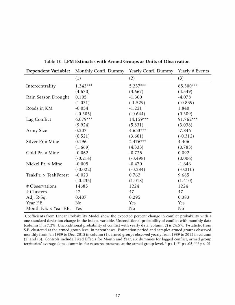
Table 10: LPM Estimates with Armed Groups as Units of Observation
Dependent Variable: Monthly Confl. Dummy Yearly Confl. Dummy Yearly # Events
(1) (2) (3)
Intercentrality 1.343*** 5.237*** 65.300***(4.670) (3.667) (4.549)
Rain Season Drought 0.105 -1.300 -4.078(1.031) (-1.529) (-0.839)
Roads in KM -0.054 -1.221 1.840(-0.305) (-0.644) (0.309)
Lag Conflict 6.079*** 14.159*** 91.762***(9.924) (5.831) (3.038)
Army Size 0.207 4.653*** -7.846(0.521) (3.601) (-0.312)
Silver Pr.×Mine 0.196 2.476*** 4.406(1.669) (4.333) (0.783)
Gold Pr. ×Mine -0.062 -0.725 0.092(-0.214) (-0.498) (0.006)
Nickel Pr. ×Mine -0.005 -0.470 -1.646(-0.022) (-0.284) (-0.310)
TeakPr. × TeakForest -0.023 0.762 9.685(-0.235) (1.018) (1.410)
# Observations 14685 1224 1224# Clusters 47 47 47Adj. R-Sq. 0.407 0.295 0.383Year F.E. No Yes YesMonth F.E. × Year F.E. Yes No No
Coefficients from Linear Probability Model show the expected percent change in conflict probability with aone standard deviation change in the indep. variable. Unconditional probability of conflict with monthly data(column 1) is 7.2%. Unconditional probability of conflict with yearly data (column 2) is 24.5%. T-statistic fromS.E. clustered at the armed group level in parentheses. Estimation period and sample: armed groups observedmonthly from Jan 1989 to Dec. 2015 in column (1), armed groups observed yearly from 1989 to 2015 in column(2) and (3). Controls include Fixed Effects for Month and Year, six dummies for lagged conflict, armed groupterritories’ average slope, dummies for resource presence at the armed group level. * p<.1, ** p< .05, *** p< .01
47
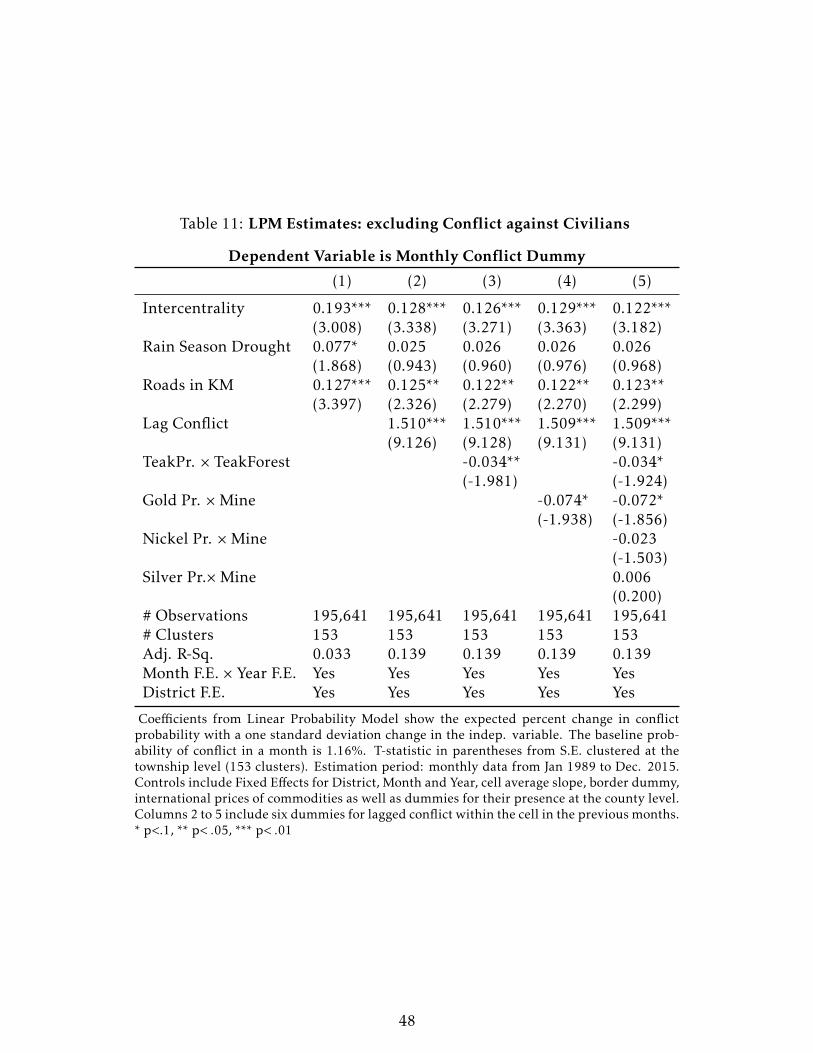
Table 11: LPM Estimates: excluding Conflict against Civilians
Dependent Variable is Monthly Conflict Dummy
(1) (2) (3) (4) (5)
Intercentrality 0.193*** 0.128*** 0.126*** 0.129*** 0.122***(3.008) (3.338) (3.271) (3.363) (3.182)
Rain Season Drought 0.077* 0.025 0.026 0.026 0.026(1.868) (0.943) (0.960) (0.976) (0.968)
Roads in KM 0.127*** 0.125** 0.122** 0.122** 0.123**(3.397) (2.326) (2.279) (2.270) (2.299)
Lag Conflict 1.510*** 1.510*** 1.509*** 1.509***(9.126) (9.128) (9.131) (9.131)
TeakPr. × TeakForest -0.034** -0.034*(-1.981) (-1.924)
Gold Pr. ×Mine -0.074* -0.072*(-1.938) (-1.856)
Nickel Pr. ×Mine -0.023(-1.503)
Silver Pr.×Mine 0.006(0.200)
# Observations 195,641 195,641 195,641 195,641 195,641# Clusters 153 153 153 153 153Adj. R-Sq. 0.033 0.139 0.139 0.139 0.139Month F.E. × Year F.E. Yes Yes Yes Yes YesDistrict F.E. Yes Yes Yes Yes Yes
Coefficients from Linear Probability Model show the expected percent change in conflictprobability with a one standard deviation change in the indep. variable. The baseline prob-ability of conflict in a month is 1.16%. T-statistic in parentheses from S.E. clustered at thetownship level (153 clusters). Estimation period: monthly data from Jan 1989 to Dec. 2015.Controls include Fixed Effects for District, Month and Year, cell average slope, border dummy,international prices of commodities as well as dummies for their presence at the county level.Columns 2 to 5 include six dummies for lagged conflict within the cell in the previous months.* p<.1, ** p< .05, *** p< .01
48

Tabl
e12
:LPM
Est
imat
es:V
ario
us
Com
mod
itie
s
Dep
end
ent
Var
iab
leis
Mon
thly
Con
flic
tD
um
my
(1)
(2)
(3)
(4)
(5)
(6)
(7)
Inte
rcen
tral
ity
0.09
6**
0.08
9**
0.09
1**
0.10
1***
0.08
8**
0.09
4**
0.09
8**
(2.5
59)
(2.3
52)
(2.4
62)
(2.6
84)
(2.3
48)
(2.4
91)
(2.5
49)
Nic
kelP
r.×
Min
e-0
.025
-0.0
40**
(-1.
590)
(-2.
551)
Silv
erP
r.×
Min
e0.
028
0.01
5(1
.314
)(0
.967
)C
opp
erP
r.×
Min
e0.
030
0.02
4(1
.350
)(1
.231
)Ir
onP
r.×
Min
e0.
052*
0.05
7*(1
.771
)(1
.933
)L
ead
Pr.×
Min
e0.
022
-0.0
01(1
.222
)(-
0.07
7)P
lati
num
Pr.×
Min
e0.
040
0.11
3***
(1.3
64)
(3.3
92)
#O
bser
vati
ons
195,
641
195,
641
195,
641
195,
641
195,
641
195,
641
195,
641
#C
lust
ers
153
153
153
153
153
153
153
Ad
j.R-
Sq.
0.16
90.
169
0.16
90.
169
0.16
90.
169
0.16
9M
onth
F.E
.×Ye
arF.
E.
Yes
Yes
Yes
Yes
Yes
Yes
Yes
Dis
tric
tF.
E.
Yes
Yes
Yes
Yes
Yes
Yes
Yes
Coe
ffici
ents
from
Lin
ear
Pro
babi
lity
Mod
elsh
owth
eex
pec
ted
per
cent
chan
gein
confl
ict
pro
babi
lity
wit
ha
one
stan
dar
dd
evia
tion
chan
gein
the
ind
ep.
vari
able
.T
heba
seli
nep
roba
bili
tyof
confl
ict
ina
mon
this
1.16
%.
T-st
atis
tic
inp
aren
thes
esfr
omS.
E.
clu
ster
edat
the
tow
nshi
ple
vel
(153
clu
ster
s).
Est
imat
ion
per
iod
:m
onth
lyd
ata
from
Jan
1989
toD
ec.
2015
.C
ontr
ols
incl
ud
eFi
xed
Effe
cts
for
Dis
tric
t,M
onth
-Yea
r,ce
llav
erag
esl
ope,
bord
erdu
mm
y,si
xdu
mm
ies
for
lagg
edco
nflic
tw
ithi
nth
ece
llin
the
pre
viou
sm
onth
s,in
tera
ctio
nsof
inte
rnat
iona
lp
rice
sof
com
mod
itie
san
ddu
mm
ies
for
thei
rp
rese
nce
atth
eco
unt
yle
vel.
*p<
.1,*
*p<.0
5,**
*p<.0
1
49
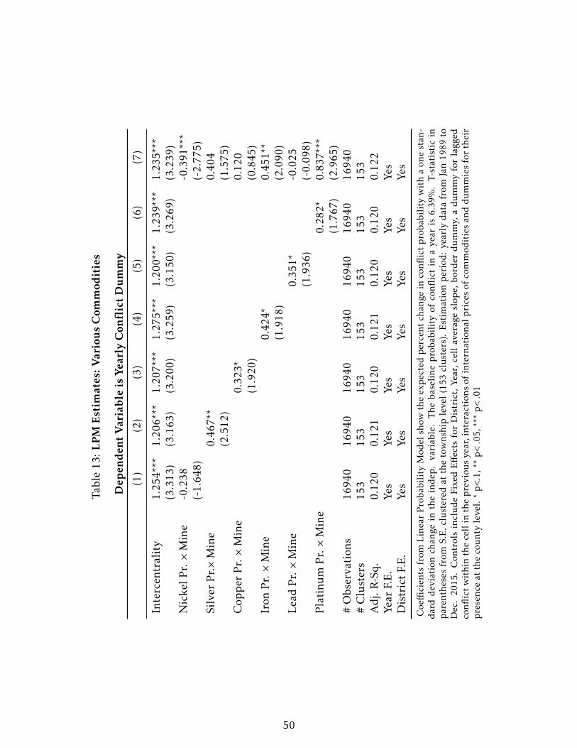
Tabl
e13
:LPM
Est
imat
es:V
ario
us
Com
mod
itie
s
Dep
end
ent
Var
iab
leis
Year
lyC
onfl
ict
Du
mm
y
(1)
(2)
(3)
(4)
(5)
(6)
(7)
Inte
rcen
tral
ity
1.25
4***
1.20
6***
1.20
7***
1.27
5***
1.20
0***
1.23
9***
1.23
5***
(3.3
13)
(3.1
63)
(3.2
00)
(3.2
59)
(3.1
50)
(3.2
69)
(3.2
39)
Nic
kelP
r.×
Min
e-0
.238
-0.3
91**
*(-
1.64
8)(-
2.77
5)Si
lver
Pr.×
Min
e0.
467*
*0.
404
(2.5
12)
(1.5
75)
Cop
per
Pr.×
Min
e0.
323*
0.12
0(1
.920
)(0
.845
)Ir
onP
r.×
Min
e0.
424*
0.45
1**
(1.9
18)
(2.0
90)
Lea
dP
r.×
Min
e0.
351*
-0.0
25(1
.936
)(-
0.09
8)P
lati
num
Pr.×
Min
e0.
282*
0.83
7***
(1.7
67)
(2.9
65)
#O
bser
vati
ons
1694
016
940
1694
016
940
1694
016
940
1694
0#
Clu
ster
s15
315
315
315
315
315
315
3A
dj.
R-Sq
.0.
120
0.12
10.
120
0.12
10.
120
0.12
00.
122
Year
F.E
.Ye
sYe
sYe
sYe
sYe
sYe
sYe
sD
istr
ict
F.E
.Ye
sYe
sYe
sYe
sYe
sYe
sYe
s
Coe
ffici
ents
from
Lin
ear
Pro
babi
lity
Mod
elsh
owth
eex
pec
ted
per
cent
chan
gein
confl
ict
pro
babi
lity
wit
ha
one
stan
-d
ard
dev
iati
onch
ange
inth
ein
dep
.va
riab
le.
The
base
line
pro
babi
lity
ofco
nflic
tin
aye
aris
6.39
%.
T-st
atis
tic
inp
aren
thes
esfr
omS.
E.c
lust
ered
atth
eto
wns
hip
leve
l(1
53cl
ust
ers)
.E
stim
atio
np
erio
d:
year
lyd
ata
from
Jan
1989
toD
ec.
2015
.C
ontr
ols
incl
ud
eFi
xed
Effe
cts
for
Dis
tric
t,Ye
ar,
cell
aver
age
slop
e,bo
rder
dum
my,
adu
mm
yfo
rla
gged
confl
ict
wit
hin
the
cell
inth
ep
revi
ous
year
,int
erac
tion
sof
inte
rnat
iona
lpri
ces
ofco
mm
odit
ies
and
dum
mie
sfo
rth
eir
pre
senc
eat
the
cou
nty
leve
l.*
p<
.1,*
*p<.0
5,**
*p<.0
1
50

A.7 Instrumental Variable: Additional Results
Table 14: Instrumental Variable Estimation: Yearly Data
Dependent Variable Yearly Conflict Dummy
OLS Red.Form 2SLS First Stage(1) (2) (3) (4)
Intercentrality 1.235*** 1.364***(3.239) (3.068)
Instrum. Intercentrality 1.195*** 0.876***(3.154) (13.745)
Adj. R-Sq. 0.121 0.120 0.121 0.532F-test 188.931Partial R-Sq. 0.35# Observations 16940 16940 16940 16940# Clusters 153 153 153 153Year F.E. Yes Yes Yes YesDistrict F.E. Yes Yes Yes Yes
Coefficients from Linear Probability Model show the expected percent change in con-flict probability with a one standard deviation change in the indep. variable. Thebaseline probability of conflict in a year is 6.39%. T-statistic in parentheses from S.E.clustered at the township level (153 clusters). Estimation period: yearly data from Jan1989 to Dec. 2015. Controls include KM of Roads within the cell, altitude, dummyfor drought during the last two months of the rain season, international prices of com-modities as well as dummies for their presence at the county level. * p<.1, ** p< .05, ***p< .01
51
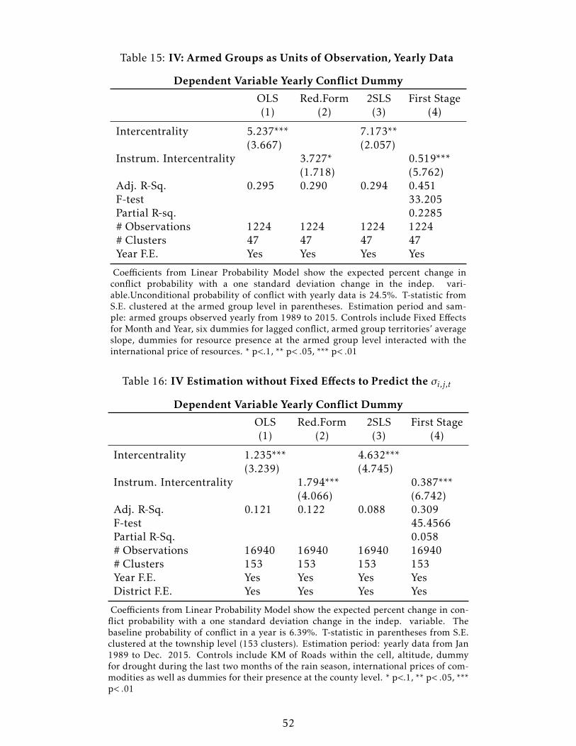
Table 15: IV: Armed Groups as Units of Observation, Yearly Data
Dependent Variable Yearly Conflict Dummy
OLS Red.Form 2SLS First Stage(1) (2) (3) (4)
Intercentrality 5.237*** 7.173**(3.667) (2.057)
Instrum. Intercentrality 3.727* 0.519***(1.718) (5.762)
Adj. R-Sq. 0.295 0.290 0.294 0.451F-test 33.205Partial R-sq. 0.2285# Observations 1224 1224 1224 1224# Clusters 47 47 47 47Year F.E. Yes Yes Yes Yes
Coefficients from Linear Probability Model show the expected percent change inconflict probability with a one standard deviation change in the indep. vari-able.Unconditional probability of conflict with yearly data is 24.5%. T-statistic fromS.E. clustered at the armed group level in parentheses. Estimation period and sam-ple: armed groups observed yearly from 1989 to 2015. Controls include Fixed Effectsfor Month and Year, six dummies for lagged conflict, armed group territories’ averageslope, dummies for resource presence at the armed group level interacted with theinternational price of resources. * p<.1, ** p< .05, *** p< .01
Table 16: IV Estimation without Fixed Effects to Predict the σi,j,t
Dependent Variable Yearly Conflict Dummy
OLS Red.Form 2SLS First Stage(1) (2) (3) (4)
Intercentrality 1.235*** 4.632***(3.239) (4.745)
Instrum. Intercentrality 1.794*** 0.387***(4.066) (6.742)
Adj. R-Sq. 0.121 0.122 0.088 0.309F-test 45.4566Partial R-Sq. 0.058# Observations 16940 16940 16940 16940# Clusters 153 153 153 153Year F.E. Yes Yes Yes YesDistrict F.E. Yes Yes Yes Yes
Coefficients from Linear Probability Model show the expected percent change in con-flict probability with a one standard deviation change in the indep. variable. Thebaseline probability of conflict in a year is 6.39%. T-statistic in parentheses from S.E.clustered at the township level (153 clusters). Estimation period: yearly data from Jan1989 to Dec. 2015. Controls include KM of Roads within the cell, altitude, dummyfor drought during the last two months of the rain season, international prices of com-modities as well as dummies for their presence at the county level. * p<.1, ** p< .05, ***p< .01
52