ISSN 1403-2473 (Print) ISSN 1403-2465 (Online)

Working Paper in Economics No. 807

Charity, Status, and Optimal Taxation: Welfarist and Non-Welfarist Approaches

Thomas Aronsson, Olof Johansson-Stenman, Ronald Wendner

Department of Economics, June 2021

1

Charity, Status, and Optimal Taxation: Welfarist

and Non-Welfarist Approaches1

Thomas Aronsson a

Olof Johansson-Stenman b

Ronald Wendner c

a Department of Economics, Umeå School of Business, Economics and Statistics, Umeå

University, Sweden

b Department of Economics, School of Business, Economics and Law, University of

Gothenburg, Sweden

c Department of Economics, University of Graz, Austria

June 2021

Abstract

This paper analyzes optimal taxation of charitable giving to a public good in a Mirrleesian

framework with social comparisons. Leisure separability together with zero transaction costs

of giving imply that charitable giving should be subsidized to such an extent that

governmental contributions are completely crowded out, regardless of whether the

government acknowledges warm glows of giving. Stronger concerns for relative charitable

giving and larger transaction costs support lower marginal subsidies, whereas relative

consumption concerns work in the other direction. A dual screening approach, where

charitable giving constitutes an indicator of wealth, is also presents. Numerical simulations

supplement the theoretical results.

Keywords: Conspicuous consumption, conspicuous charitable giving, optimal taxation,

public good provision, warm glow, multiple screening.

JEL Classification: D03, D62, H21, H23

1 The authors would like to thank Tommy Andersson, Nathalie Bolh, Dawei Fang, David Granlund, Randi

Hjalmarsson, Etienne Lehmann, Mikael Lindahl, Volker Meier, Katarina Nordblom, Tomas Sjögren, and Harald

Uhlig for very helpful comments and suggestions. The paper has been presented at seminars at the University of

Arizona, the Free University, Berlin, the University of Gothenburg, Linnaeus University, University of

Osnabrück, Umeå University, and the University of Vermont, as well as at the 111th Annual Conference of the

National Tax Association in New Orleans 2018, the 2019 Meeting of the of the European Public Choice Society

in Jerusalem, and the 75th Annual Congress of the International Institute of Public Finance 2019 in Glasgow.

The authors would like to thank the participants for valuable discussions. Research grants from The Marianne

and Marcus Wallenberg Foundation (MMW 2015.0037) are gratefully acknowledged.

2

What is the optimal tax treatment of charitable giving? Individuals and organizations donate

substantial amounts to charities, not least in the United States where charitable giving

amounted to about $450 billion, or more than 2% of GDP, in 2019 (Giving USA, 2020). The

bulk of these donations can be described as voluntary contributions to public goods or

community services, e.g., religious and environmental organizations and research, education,

and public-society benefit charities (Giving USA, 2020). Thus, the importance of the above

question is a given. The purpose of the present paper is to answer the question by integrating

the tax treatment of charitable giving in a Mirrleesian model of optimal redistributive taxation.

That the answer is non-trivial is indicated by the fact that tax policies related to charitable

giving vary largely both between countries and within countries over time (Fack and Landais,

2012).

To our knowledge, the present study is the first to integrate voluntary contributions to

a public good, to which there is also potential public provision, into a continuous-type

Mirrleesian framework. In doing so, we also distinguish between a conventional welfarist

government that respects all aspects of consumer preferences and forms the social objective

thereupon, and a non-welfarist government that does not attach any social value to the warm

glow of giving. Each such government collects revenue and redistributes through a nonlinear

tax based on both gross income and charitable giving, implying that the set of available policy

instruments reflects information limitations rather than a priori restrictions on the tax

instruments. This is crucial and allows us to derive sharper and more easily interpretable

policy rules than would otherwise be possible. For example, if the utility functions are weakly

leisure separable (a common assumption in the optimal taxation literature), and in the absence

of any transaction costs of charitable giving (as in previous literature; see below), a welfarist

government would subsidize charitable contributions to such an extent that they completely

crowd out governmental provision of the public good. The intuition is based on logic similar

to the Atkinson and Stiglitz (1976) theorem: the marginal subsidies on charitable giving are in

this case based on a first-best policy rule guided solely by concerns for economic efficiency.

Such a policy favors charitable giving over public provision, since the former comes with the

additional benefit of warm glow to the givers.

Even more strikingly, we show that this complete crowding-out result continues to

hold also when the government is non-welfarist and does not attach any social value to the

warm glow of giving. The logic here is that subsidizing charitable giving for high-income

earners constitutes a cost-efficient means of redistribution. Furthermore, and regardless of

whether the government values the warm glow of giving, the complete crowding out result

3

remains if charitable giving and private consumption are driven by concerns for social status.

We present sufficient conditions for complete crowding out in the general case where the

utility functions are not necessarily leisure separable.

After a brief review of earlier research on the optimal tax treatment of voluntary

contributions to public goods in Section I, Section II presents our Mirrleesian (1971) model

using a modified version of Diamond’s (1998) and Saez’s (2001) ABC formulation, extended

with private and public contributions to a public good. An important novelty is that we allow

for transaction costs of charitable giving, such that a fraction of the contribution is lost in the

process. Such costs play a critical role by reducing the marginal subsidies to charitable giving,

and (if the costs are not too small) imply that the government should also contribute directly

to the public good in accordance with a modified Samuelson rule. Under leisure separability,

a welfarist government implements a flat rate subsidy on charitable giving, whereas a non-

welfarist government implements income-varying marginal subsidies.

Section III generalizes the model further to encompass conspicuous charitable giving

and conspicuous consumption, respectively, such that people derive well-being from giving

more to charity and consuming more than referent others, and vice versa.2,3 The model then

contains three simultaneous externalities: i) A contribution to the public good by an individual

increases the size of the public good and thus induces a corresponding benefit for all

individuals. ii) The same contribution also decreases others’ relative contribution, and

correspondingly decreases their utility. iii) Increased consumption by an individual reduces

the relative consumption of all others, and therefore decreases their utility. The strength of the

concerns for relative charitable giving typically works in the direction of supporting lower

marginal subsidies on charitable giving, whereas the strength of the concerns for relative

consumption works in the other direction. An interesting exception arises if zero bunching in

charitable giving is sufficiently prevalent, in which case an increase in the positional gifts

externality may actually motivate a higher marginal subsidy (or a lower marginal tax) on

2 Several studies suggest that charitable giving is a means of signaling status or prestige (e.g., Glazer and Konrad,

1996; Harbaugh, 1998).

3 A large literature suggests that people derive well-being from their relative consumption or income. See, e.g.,

Johansson-Stenman et al. (2002), Solnick and Hemenway (2005), and Carlsson et al. (2007) for evidence based

on questionnaire-experimental research, and Easterlin (2001), Blanchflower and Oswald (2004), Ferrer-i-

Carbonell (2005), and Clark and Senik (2010) for evidence based on happiness research. For theoretical work on

tax and expenditure policy in the presence of relative income or consumption concerns, see, e.g., Boskin and

Sheshinski (1978), Oswald (1983), Dupor and Liu (2003), Ljungqvist and Uhlig (2000), Aronsson and

Johansson-Stenman (2008, 2010), Wendner and Goulder (2008), and Eckerstorfer and Wendner (2013).

4

charitable giving. For governmental contributions to the public good and the marginal tax

treatment of charitable giving, respectively, leisure separability simplifies the optimal policy

rules dramatically, again based on logic similar to the Atkinson and Stiglitz (1976) theorem.

In the general case where leisure separability no longer necessarily applies, we demonstrate

how the redistributive components of these policy rules can be written directly in terms of the

optimal marginal income tax. This way of writing the policy rules is novel and further

emphasizes the roles of governmental provision to the public good and the marginal

subsidy/tax on charity as supplemental instruments for income redistribution.

Section IV presents yet another generalization in the form of a dual screening model

where individuals now differ in two dimensions: ability (gross wage), as before, and wealth,

where wealth is also unobservable to the government and independent of the labor supplied.

Assuming that charitable giving is a normal good, we use it as a second screening device in

order to redistribute from individuals with higher ability and higher wealth. We express the

optimal policy rules using a two-dimensional ABC formulation, where the positional

externalities caused by concerns for relative consumption and relative charitable giving enter

the policy rules in a way similar to the simpler model in Section III. However, since the logic

behind the Atkinson-Stiglitz theorem is not applicable to the screening mechanism in the

wealth dimension, leisure separability will no longer imply the same drastic simplifications of

the policy rules.

Section V supplements the theoretical results with extensive numerical simulations

based on specific functional forms for the utility functions and the ability distribution. Section

VI concludes the paper, whereas proofs are presented in the Appendix.

I. A Brief Literature Review on Optimal Taxation and Charitable Giving

A number of studies have examined the policy implications of charitable giving in models of

optimal (albeit not Mirrleesian) taxation, where the donations to charity are described in terms

of voluntary contributions to a public good (e.g., Feldstein, 1980; Warr, 1982; Saez, 2004;

Diamond, 2006; Blumkin and Sadka, 2007).4 In a model with optimal linear taxation, Saez

(2004) shows that the optimal subsidy on voluntary contributions can be expressed as a sum

of three elements: the positive externality that each contributor imposes on other people (as in

4 There is also a much smaller literature modeling charitable giving as direct redistribution from richer to poorer

groups; see Atkinson (1976), Kaplow (1995), and Aronsson, Johansson-Stenman, and Wendner (2019). Whereas

the former two studies focus on the tax treatment of such gifts in a first-best environment, the latter examines

optimal redistributive income taxation in a two-type model where the high-ability type can give an income

transfer to the low-ability type.

5

Warr, 1982), the price sensitivity of the contribution good, and the extent to which direct

public contributions crowd out private contributions. Diamond (2006) uses a model of

optimal nonlinear taxation developed by Diamond (1980), where the jobs available differ

among skill types and the hours of work at a given job are fixed, to derive a second-best

argument for marginal subsidies to charitable giving at the top of the income distribution. He

shows that voluntary contributions by high earners relax the incentive compatibility constraint

and hence motivate a marginal subsidy. In our Mirrleesian framework, the corresponding

mechanisms can go in either direction (depending on whether the marginal valuation of

charitable giving increases or decreases with the time spent on leisure) and would vanish

under leisure separability.

Diamond (2006) also argues against using warm-glow preferences as a basis for social

cost benefit analysis since the warm glow is likely to be context dependent. Furthermore, by

recognizing warm glow as a source of benefit, there may also be reasons to devote resources

to produce the contexts in which warm glow arises, which is not necessarily the best use of

resources. Further arguments against including such benefits are related to the social pressure

to contribute (e.g., DellaVigna et al., 2012). Yet, see Kaplow (1998) and Kaplow and Shavell

(2001) for arguments suggesting that benefits arising from the warm glow of giving should

indeed be accounted for. We therefore follow Diamond (2006) and present results reflecting

both when the government values and when it does not value the warm glow of giving.5

Blumkin and Sadka (2007) examine a status motive for charitable giving as well as tax

policy implications thereof. They consider a model where charitable donations signal status,

while neglecting the warm-glow motive addressed by Saez and Diamond in their respective

studies. By examining the welfare effect of introducing a small tax on charitable giving when

the income tax is optimal, they find that the optimal tax on charitable giving is non-negative;

it is positive if status concerns lead to overprovision of the public good compared with the

Samuelson condition and zero otherwise. In the present paper, their finding can be seen as a

special case.

5 One could argue, e.g., based on Harsanyi (1982), that the government should not value relative consumption

effects either; see Aronsson and Johansson-Stenman (2018) for implications in terms of optimal income taxation

in a two-type model. The major qualitative results continue to hold for this extended version of non-welfarism,

and are available from the authors upon request.

6

II. A Mirrleesian Model with Charitable Giving and Public Goods

Consider an economy with linear production and competitive markets, implying that marginal

productivity, w, reflects an ability-specific, fixed wage rate per unit of labor, which we refer

to as ability in what follows. Ability is distributed continuously, and the population is fixed

and normalized to one, i.e., 0

( ) 1f w dw

. The size of the public good, G, depends on the

sum of individual contributions, g, and the amount provided directly by the government, GovG .

Contrary to earlier studies on the optimal tax treatment of charitable contributions to

public goods (see Section I), we introduce a transaction cost attached to charitable giving. We

formalize this cost in a simple way by assuming a potential discrepancy between the donation

and its contribution to the public good, such that the overall size of the public good is given as

follows:

0

(1 ) ( )Gov

wG G g f w dw

, (1)

where 1 thus reflects the transaction cost. Since there may be transaction costs also for

governmental provision of public goods, it is natural to interpret as a measure of additional

transaction costs associated with charitable giving. In this perspective, one cannot rule out

that 0 . Yet, for simplicity, in the subsequent analysis we focus on the case where 0

(where interpretations thus change accordingly when 0 ). One may also interpret more

broadly as reflecting a less optimal distribution of public goods from society’s point of view.

Individuals are endowed with one unit of time and supply 0 1l units of labor.

Their utility depends on consumption, c , labor, l (and hence leisure, 1-l), and the overall level

of the public good, G. In addition, it depends on their own charitable contribution to the

public good, g , implying a corresponding warm glow (Andreoni, 1989):6

( , , , ; )w w w wu u c l g G w . (2)

We assume that ( )u is twice continuously differentiable, increasing in c , g , and G ,

decreasing in l , and strictly concave.7 We also assume that charitable giving is a normal good.

Following, e.g., Saez (2004) and Blumkin and Sadka (2007), individuals are assumed to be

6 This should not be interpreted to mean that people solely care about how much they contribute and not about

the public good to which they contribute. Thus, if we were to extend the model to include several public goods,

which is quite straightforward, the warm glow per dollar contributed may differ among charities.

7 Alternatively, one may assume that people derive utility from their net contribution to the public good,

(1 )g . Since is exogenous to the individual, we can still think of equation (2) as a reduced form. All

qualitative insights would hold also with this alternative formulation.

7

atomistic agents by treating the level of the public good, G, as exogenous.8 In Section III, we

make the analogous assumption that individuals treat externalities as exogenous. The final

argument in the utility function reflects that we allow for continuous preference

heterogeneity. The preferences may be very different for, say, individuals at the 75th

percentile of the income distribution compared with those at the 25th percentile, but the

preference differences are small for small differences in ability and vanish completely without

any ability differences. For later use, the following definition will prove useful:

Definition. The utility function is denoted leisure separable if it can be written

( ( , , ; ), ; )w w w wu V k c g G w l w .

Leisure separability thus implies that the marginal rates of substitution between c , G, and g

are independent of labor (and hence leisure) for all individuals. Note that this assumption is

weaker than additive separability, which is often assumed (see e.g., Tuomala, 2016). The

individual budget constraint implies that the sum of private consumption and charitable giving

equals gross income, y wl , minus the taxes paid:

( , )w w w w wy T y g c g , (3)

where ( , )T y g is a general, nonlinear tax function through which the tax payment depends on

both gross income and charitable giving. Each individual chooses consumption, work hours,

and charitable giving to maximize utility given by (2) subject to their respective budget

constraint (3). In addition to (3), an interior solution satisfies the individual first-order

conditions for labor supply and charitable giving:

( )

( ) ( )

, ( )1

ww wl

l c yw

c

uMRS w T

u ;

( )

( ) ( )

, ( )1

w

gw w

g c gw

c

uMRS T

u . (4)

Single subscripts attached to the utility function or tax function reflect partial derivatives

(unless being w), where yT denotes the marginal income tax and

gT the marginal tax or

subsidy (if negative) on charitable giving; ( )w refers to ability type.

The social welfare function is a generalized utilitarian welfare function as follows:

0( ) ( )wW u f w dw

, (5)

8 This is in contrast to Bergstrom, Blume, and Varian (1986), where individuals treat G as endogenous. In their

study, an individual’s contribution is not negligible to G.

8

where is (weakly) concave. We will consider two versions of social welfare: a conventional

welfarist objective where the government takes individual utility at face value (as in [5]) and a

non-welfarist version where the government does not value utility changes caused by the

warm glow of giving. Whether the government is welfarist or not, it faces the same resource

constraint and incentive compatibility constraints. The resource constraint means that the

aggregate production equals the sum of aggregate private consumption and charitable giving

plus the governmental contributions to the public good,

0 0( ) ( ) ( ) Gov

w w wwl f w dw c g f w dw G

. (6)

We assume that the government observes income and charitable giving at the individual level,

whereas ability is private information. The incentive compatibility constraints serve to prevent

individuals of any type w from mimicking the ability type just below them in terms of

observable income and charitable giving,

( )/ /w

w w ldu dw l u w . (7)

Our tax instruments and informational assumptions imply that the government can implement

any desired combination of labor supply, consumption, and charitable giving for each type

subject to the resource and incentive compatibility constraints. Therefore, we follow much

earlier work in formulating the social decision problem as a direct decision problem

throughout the paper. In doing so, we treat utility, wu , as a state variable, while wl , wg , and

GovG are control variables. Consumption, wc , is defined by the inverse of the function ( )u in

equation (2) such that ( , , , ; )w w w wc h l g G u w , the properties of which are ( ) ( )

,

w w

l l ch MRS ,

( ) ( )

,

w w

g g ch MRS , ( ) ( ) ( ) ( )

, /w w w w

G G c G ch MRS u u , and ( ) ( )1/w w

u ch u , where a subscript attached

to the function ( )h denotes a partial derivative. The policy rules for marginal income taxation

and the marginal subsidization/taxation of charitable giving can then be derived by combining

the private and social first-order conditions; thus, following convention in the optimal

taxation literature, we implicitly assume that underlying convexity assumptions are fulfilled to

ensure that the second-order conditions for a unique social optimum hold.

A. Welfarist Government

The welfarist government maximizes the social welfare function (5) subject to (6), (7), and

the non-negativity constraint 0GovG . 9 The non-negativity constraint on governmental

9 We choose not to include non-negativity constraints on charitable giving here. If individuals do not engage in

social comparisons with respect to charitable giving, such non-negativity constraints do not affect the policy rule

9

contributions plays an important role for the marginal tax treatment of charitable giving. Let

, ,( / )( / )lc

l l c l cMRS l l MRS represent the elasticity of ,l cMRS with respect to l and let

( )'( ) /w

w w cu u denote the welfare weight attached to type w, where is the Lagrange

multiplier on the resource constraint. Following Diamond’s (1998) ABC formulation, we can

then define10

( )1 ,lc

w l wA (8a)

( )( )

( )1 exp exp ,

1 ( )

ms smgclc m

w w m

w w w

MRSMRS dy f sB dg ds

c m c F w

(8b)

1 ( )

( )w

F wC

wf w

. (8c)

Equations (8a)–(8c) are the building blocks of the policy rule for marginal income taxation

and will be interpreted below. To simplify the presentation, let , ,( / )( / )Gc

l G c G cMRS l l MRS

and , ,( / )( / )gc

l g c g cMRS l l MRS represent the elasticities of ,G cMRS and

,g cMRS with respect

to labor, and let 0S denote society’s net marginal cost of public good provision in the absence

of any direct contribution to the public good by the government (to be formalized below). We

can now summarize the optimal policy rules for marginal income taxation, governmental

provision of the public good, and the marginal tax treatment of charitable giving (where (w)

as subscript or superscript reflects dependency on w). In order to simplify presentation and the

corresponding interpretations, we start with the special case of leisure separability and then

present the results for the general non-separable case.11

underlying the optimal tax treatment of charitable giving. We introduce non-negativity constraints in Section III,

where individuals derive well-being from their relative charitable giving.

10 Under leisure separability, we can express A in the same way as Saez (2001) so 1 (1 ) /lc u c

lA ,

where u and

c are the uncompensated and compensated elasticity, respectively, of l with respect to the

marginal wage rate derived under a linearized budget constraint. Under quasi-linearity, as in Diamond (1998),

(8b) simplifies to (1 ) ( ) / (1 ( ))w ww

B f s F w ds

.

11 The marginal income tax rates in (i) apply for those supplying labor (as in e.g. Saez 2001), and the marginal

subsidies/taxes on charitable giving in (ii) and (iii) apply for those contributing to charity. In the numerical

simulations, we address zero-bunching both in terms of work hours and charitable giving, and also illustrate the

income ranges where people contribute to charity and where they do not.

10

Proposition 1a. For a welfarist government, and if the utility functions are leisure separable,

(i)–(iv) hold:

(i)

( )

( )1

w

y

w w ww

y

TA B C

T

.

(ii) If 0GovG , then ( )

,0

( ) 1w

G cMRS f w dw

and ( ) 1w

gT .

(iii) If 0GovG , then ( ) 01 (1 )w

gT S .

(iv) If 0 , then 0GovG .

The ABC rule for marginal income taxation in (i) and the policy rule for public good

provision in (ii), where the marginal rate of transformation between public and private goods

is equal to one, take the same general forms as in the absence of any charitable giving,

although B is modified with an additional income effect in the g-dimension. The variable A is

interpretable as an efficiency mechanism based on behavioral responses, B reflects the desire

for redistribution, and C reflects the thickness of the upper tail of the ability distribution.

Based on logic similar to the Atkinson-Stiglitz (1976) theorem, the policy rule for public good

provision reduces to the standard Samuelson condition under leisure separability, as in the

seminal contributions by Christiansen (1981) and Boadway and Keen (1993), both of which

are based on models without private contributions to the public good.

The policy rules for gT in results (ii) and (iii) of the proposition refer to the marginal

tax treatment of charitable giving, i.e., the main interest of the present paper. Consider first

the special case without any transaction costs ( 0 ), which is the case examined in all

existing literature dealing with tax policy implications of charitable giving. Then, if 0GovG ,

(ii) would imply 1gT , i.e., a 100% marginal subsidy to charitable giving. Obviously, such

a policy mix cannot be optimal, since utility increases monotonically in charitable giving.

Instead, this special case implies 0GovG according to (iv). (Note that the condition in [iv],

0 , is sufficient but not necessary for 0GovG .) Thus, it is optimal for the government not

to contribute at all to the public good! The intuition is that charitable giving provides an

additional welfare benefit due to the warm glow of giving that does not follow from

governmental provision. The policy rule for the marginal subsidy to charitable giving is then

correspondingly modified and given in (iii), where

0 ( )

,0

0

1 ( ) 0Gov

w

G cG

S MRS f w dw

measures the discrepancy between society’s marginal cost and marginal benefit of

governmental provision evaluated at 0GovG . In technical terms, 0S is the Lagrange

11

multiplier of the non-negativity constraint for GovG over the Lagrange multiplier of the

resource constraint.12 Thus, the government reduces the marginal subsidy in order to try to

avoid that voluntary contributions lead to overprovision of the public good relative to the

Samuelson condition, and it does so by choosing ( ) 01w

gT S for all w when 0 .

It is interesting to compare this policy rule with a corresponding result by Saez (2004),

who derives optimal linear income and charitable giving taxation. Such a comparison is

complicated by the fact that the linearity restriction (in addition to the other constraints)

typically requires additional simplifying assumptions to obtain policy rules comparable with

those derived under nonlinear taxation. When Saez makes a number of additional

assumptions,13 he finds that the tax rate on charitable giving is equal to -1, i.e., a 100%

subsidy; thus, there is no additional 0S term, as in our case. Yet, we can resolve this puzzle

by noting that Saez does not explicitly assume utility to be monotonically increasing (as we

do), but only non-decreasing, in charitable giving. Therefore, it is possible to interpret the

extreme 100% subsidy as resulting from a situation where the marginal utility of charitable

giving equals zero beyond a certain level of giving. This opens up for the possibility that the

voluntary contributions are small enough to imply that direct governmental provision would

still be optimal.14 Consequently, the non-negativity constraint for governmental provision

does not bind in this case, and a 100% subsidy rate would be perfectly logical. The same

result would follow in our model. Moreover, if utility would be monotonically increasing in

charitable giving in the model by Saez, the policy rule 01 S would result there as well.15

12 See the Appendix for details.

13Specifically: i) there are no income effects on earnings, ii) the aggregate gross income is independent of both

the public good and the subsidy on charitable giving, iii) the compensated supply of contributions does not

depend on the income tax, and iv) the aggregate voluntary contribution is reduced by exactly one unit for each

additional unit of governmental provision. The results in the present paper, in contrast, hold regardless of

whether these assumptions are fulfilled or not.

14 However, when individuals are indifferent about whether or not to contribute more to the public good (despite

a 100% subsidy), the individual optimization problem does not have a unique solution. For the latter we would

also need an additional assumption that all individuals prefer not to contribute more in this situation.

15 The first-order condition for governmental provision of the public good is given by equation (5) in Saez

(2004), which assumes that this contribution is positive. By adding the assumption that utility is monotonically

increasing (instead of non-decreasing) in charitable giving, and explicitly recognizing the non-negativity

constraint on governmental contributions, it is straightforward to use Saez’s model to show that the subsidy to

charitable giving becomes 01 S , where 0S is given by the Lagrange multiplier of the non-negativity constraint

over the Lagrange multiplier of the resource constraint.

12

Proposition 1a also implies that if 0 and sufficiently large, the governmental

contribution to the public good is positive and the marginal subsidy attached to charitable

giving is based on the policy rule in (ii). It is also immediately obvious from (ii) and (iii) that

leisure separability implies that the marginal subsidy on charitable giving is the same for all

contributors. Thus, contrary to the marginal income tax rate that typically varies with the

gross income, the optimal marginal subsidy on charitable giving is in this case independent of

gross income (and also of the individual’s contribution).

Finally, and again by analogy to the Atkinson-Stiglitz (1976) theorem, leisure

separability means that the policy rule for gT takes the same form as in a first-best setting

without informational asymmetries. In other words, the marginal tax treatment of charitable

giving is guided by economic efficiency, while redistribution is dealt with through the income

tax.

If the utility functions are not leisure separable, the policy rules for GovG and gT in

Proposition 1a no longer apply. Proposition 1b presents the results for the general case, which

also includes non-separable preferences:

Proposition 1b. For a welfarist government, (i)–(iv) hold:

(i)

( )

( )1

w

y

w w ww

y

TA B C

T

.

(ii) If 0GovG , then

( )

( )( ) ( )

, ( ) , ( )0 0( )

1 ( ) 1 ( ) 11 1

Gc w

l w yw Gc w

G c l w w w G c lc w

l w y

TMRS B C f w dw MRS f w dw

T

,

( )

( )( ) ( ) ( )

( ) , , ( )

( )

1 11 1

gc w

l w yw gc w w

g l w g c w w g c lc w

l w y

TT MRS B C MRS

T

.

(iii) If 0GovG , then

( )

( )( ) 0 ( ) 0 ( )

( ) , , ( )

( )

1 (1 ) 1 (1 )1 1

gc w

l w yw gc w w

g l w g c w w g c lc w

l w y

TT S MRS B C S MRS

T

.

(iv) If 0 and ( ) 0gc

l w for some w for which 0wg , then 0GovG .

The policy rule for the marginal income tax remains the same as under leisure separability

(although the values of the ABC-factors will of course vary with respect to underlying

assumptions). However, the policy rules for GovG and gT in (ii) and (iii) differ from their

counterparts in Proposition 1a through terms proportional to the behavioral elasticities Gc

l

and gc

l , respectively. These additional components arise because the public good and the

marginal subsidy/tax on charitable giving now supplement the income tax as instruments for

13

income redistribution, which explains the interaction between the behavioral elasticities and

the product BC. To further emphasize how GovG and gT interact with the marginal income tax

policy, in the expression after the second equality we present a second variant of each such

policy rule where the behavioral elasticity is proportional to / (1 )y yT T . Thus, the absolute

value of this redistributive component increases with the marginal income tax rate, ceteris

paribus. Another implication of relaxing the separability assumption is that the marginal

subsidy/tax on charitable giving typically varies with the before-tax income (which it did not

under leisure separability).

The last term on the right-hand side of (both versions of) the policy rule for gT in (ii)

reflects the government’s incentive to relax the incentive compatibility constraints by

exploiting how individuals’ marginal valuation of charitable giving varies with leisure time

for a given disposable income (which was ruled out under leisure separability). If 0gc

l ,

charitable giving becomes more valuable relative to consumption when leisure increases

(labor decreases). Due to the conventional tax wedge, people have incentives to consume too

much (untaxed) leisure, meaning that the government has an incentive to subsidize charitable

giving at a lower marginal rate, and vice versa if 0gc

l .

The policy rule for gT in (iii), where 0GovG at the second-best optimum, extends in

the same general way (compared with the leisure-separable case in Proposition 1a). The factor

reflecting the discrepancy between society’s marginal cost and marginal benefit of public

good provision, 0S , will correspondingly be modified due to non-separability (and can be

written in terms of either the BC product or the marginal income tax) as follows:

( )

( )0 ( ) ( )

, ( ) , ( )0 00 ( )

0

1 1 ( ) 1 1 ( ) 01 1Gov

Gov

Gc w

l w yw Gc w

G c l w w w G c lc wG l w y

G

TS MRS B C f w dw MRS f w dw

T

.

Result (iv) in Proposition 1b focuses on the case where 0 and generalizes (iv) in

Proposition 1a (where ( ) 0gc

l w for all w due to leisure separability). In the absence of any

transaction costs, a sufficient condition for 0GovG is that ( ) 0gc

l w for some w for which

0wg ; hence, ( ) 0gc

l w need not hold for all w. The intuition is that if individuals for whom

( ) 0gc

l w can be made to contribute one more unit of the public good, there will be an

additional positive social net benefit compared with a one unit provision by the government. 16

16 Result (iv) gives a sufficient (not necessary) condition here as well. Note that increased charitable giving by

type w leads to a relaxation (tightening) of the incentive compatibility constraint for this type if ( )

0 ( 0)gc

l w .

14

We can also see that the relaxation of the separability assumption leads to a similar

modification of the policy rule for governmental provision in (ii), where the additional term

depends on how the marginal willingness to pay for the public good varies with leisure time.

While this general insight is well known, see, e.g., Christiansen (1981) and Boadway and

Keen (1993), we are not aware of any previous formulation of the policy rule for public good

provision expressed in terms of either the BC factor or the optimal marginal income tax.

Taken together, the redistributive elements of the policy rules for GovG and gT , which

reflect their usefulness as instruments for relaxation of the incentive compatibility constraints,

can be written in terms of estimable elasticities ( Gc

l , gc

l , and lc

l ) and the marginal income

tax rates. In particular, note that the higher the marginal income tax rates, the greater the

influence of these elements in the policy rules, ceteris paribus. This is intuitive: the higher the

marginal income tax rates, the more costly the redistributive income tax policy, and the

greater the need to use GovG and gT as supplemental instruments for redistribution.

B. Non-Welfarist Government

The non-welfarist government would like individuals to behave as if they do not derive well-

being from the warm glow of giving. Consequently, the government imposes a “laundered”

utility function on each individual of any ability w,

( , , , ; ) ( , , ; )n

w w w w w wu u c l g G w c l G w , (9)

where the non-welfarist government treats charitable giving as exogenous and attaches no

social value to changes in warm glow; yet, in equilibrium we have w wg g , meaning that (2)

and (9) take the same value. Therefore, the social welfare function in equation (5) is now

replaced with

0( ) ( )n n

wW u f w dw

. (10)

Compared with the welfarist model examined above, the optimal control problem is modified

in the sense that (10) replaces (5), and (9) appears as an additional Lagrange constraint. Thus,

Thus, it would actually suffice to assume that there are contributing individuals for whom ( )

gc

l w is either non-

negative or sufficiently small in absolute value, such that the welfare effect through the incentive compatibility

constraint, if negative, is not large enough to outweigh the positive welfare effect through the warm glow of

giving. Corresponding remarks can be made on subsequent results concerning zero public provision, i.e., result

(iii) of Proposition 2b and result (iv) of Proposition 3b.

15

n

wu is treated as an additional state variable here (see also the Appendix). The remaining

constraints are the same as in the welfarist model, since the true utility functions still drive

individual behavior.

The policy rules for marginal income taxation and governmental public good

provision are the same as in the welfarist case, but the marginal tax treatment of charitable

giving now changes. We will again for presentational reasons start with the leisure-separable

case. Let ( ) ( / )( / )c w w w w wc c represent the (negative of the) elasticity of the welfare

weight with respect to consumption,17 and let ( ) ( )

( ) , ,( / )( / )gc w w

c w g c w w g cMRS c c MRS denote the

elasticity of the marginal willingness to pay for warm glow with respect to consumption. We

can then present the following results:

Proposition 2a. For a non-welfarist government, and if the utility functions are leisure

separable, (i)–(iv) hold:

(i) If 0GovG , then ( ) ( )

,1w w

g w g cT MRS .

(ii) If 0GovG , then ( ) 0 ( )

,1 (1 )w w

g w g cT S MRS .

(iii) For 0wg , ( )w

gT satisfies ( ) 0( 0)w

g wT y iff ( ) ( )( ) gc

c w c w

.

(iv) If 0 , then 0GovG .

The policy rules presented in (i) and (ii) of Proposition 2a differ from their counterparts in the

welfarist case, Proposition 1a, due to the appearance of the last term on the right-hand side

(i.e., the component proportional to w ). This component appears because individuals value

the warm glow of giving while the government does not, meaning that the government will

adjust the incentive structure accordingly. The welfare weight w reflects that redistribution is

costly, and that it is socially preferable for this reason that high-income individuals rather than

low-income individuals contribute to charity.

This additional component in the policy rule also explains (iii) in the proposition,

since leisure separability (where 0gc

l ) implies that all marginal tax components are

constant except this final term. Thus, contrary to the corresponding policy rule under

welfarism, the marginal subsidy on charitable giving typically varies with gross income here:

the marginal subsidy increases in the gross income (and thus in the disposable income and

ability) if( ) ( )

gc

c w c w

, and vice versa. Consider the special case with a utilitarian social

17 For example, in the utilitarian case,

( )c w

would reflect the curvature of the cardinal utility function, as

measured by the coefficient of relative risk aversion.

16

welfare function where ( )c w

reflects the curvature of the cardinal utility function, as

measured by the coefficient of relative risk aversion (or the elasticity of the marginal utility of

consumption). Let us also assume that utility varies logarithmically with consumption,

corresponding to a constant coefficient of relative risk aversion equal to one. Then the optimal

marginal subsidy increases with income if ( ) 1gc

c w (and vice versa), i.e., if the marginal

willingness to pay for warm glow increases more than proportionally with private

consumption; this case is illustrated numerically in Figure 1, Section V.

That result (iv), which implies complete crowing out of governmental provision under

zero transaction costs and leisure separability, holds also in the non-welfarist case may seem

surprising at first thought, since the non-welfarist government attaches no social value to

warm glow. In addition, leisure separability eliminates all welfare effects of charitable giving

related to the incentive compatibility constraints (as it also did in the welfarist case). However,

there are distributional reasons for the non-welfarist government to prefer charitable giving to

public contributions. In this case, there is a social net cost if low-income people ( 1w )

contribute and a social net benefit if high-income people ( 1w ) do. By combining the

marginal tax/subsidy rule for charitable giving with the private first-order condition, it is easy

to see that only individuals for whom 1w will contribute at the optimum and thus generate

welfare gains in terms of a lower social cost of redistribution, while there are no

corresponding benefits from governmental provision. Proposition 2b presents the results for

the general utility function (2), which does not assume leisure separability:

Proposition 2b. For a non-welfarist government, (i)–(iii) hold:

(i) If 0GovG , then ( ) ( ) ( )

, ( ) ,

( )

( )( ) ( )

, , ( )

( )

1

11 1

w w gc w

g w g c l w g c w w

gc w

l w yw w

w g c g c lc w

l w y

T MRS MRS B C

TMRS MRS

T

.

(ii) If 0GovG , then

( ) 0 ( ) ( )

, ( ) ,

( )

( )0 ( ) ( )

, , ( )

( )

1 (1 )

1 (1 )1 1

w w gc w

g w g c l w g c w w

gc w

l w yw w

w g c g c lc w

l w y

T S MRS MRS B C

TS MRS MRS

T

(iii) If 0 and ( ) 0gc

l w for some w for which 0wg , then 0GovG .

We observe from results (i) and (ii) that the modifications due to non-separable utility take the

same form as under welfarism. Thus, also under non-welfarism, if 0 ( 0)gc

l , such that

17

charitable giving becomes more (less) valuable relative to consumption when leisure

increases, ceteris paribus, the government has an incentive to subsidize charitable giving at a

lower (higher) marginal rate. By analogy to the marginal tax treatment of charitable giving

under welfarism, we can write the new redistributive component of the policy rule for gT in

terms of either the BC factors or the marginal income tax rates.

The condition for when zero governmental provision of the public good is optimal,

given in result (iii), generalizes to the same condition as in Proposition 1b. The intuition

follows by combining the reasoning behind Propositions 1b and 2a. Essentially, if individuals

for whom ( ) 0gc

l w can be made to contribute one more unit of the public good, there will be

an additional social net benefit compared with governmental provision. This is because the

social cost of redistribution through charitable giving is lower than through a corresponding,

and tax funded, increase in GovG .

III. Incorporating Preferences for Relative Giving and Relative Consumption

In Section II, we made the conventional assumption that utility depends only on the

individual’s own consumption and charitable giving (in addition to leisure time and the public

good). We will now assume that individuals also derive well-being from their relative

consumption and relative charitable giving. This means that individuals impose positional

externalities on one another. Following the bulk of earlier research on optimal taxation and

relative consumption, we start with the most common comparison form, the mean-value

comparison, which in our case means that individuals compare their own consumption with

the average consumption and their own charitable giving with the average charitable giving.

At the end of this section, we discuss some alternative comparison forms and the implications

thereof.

A. The model

Extending the utility function to accommodate relative consumption and relative charitable

giving, equation (2) is now replaced with

( , , , , , ; ) ( , , , , , ; )w w w w w w w w wu v c l g c g G w u c l g c g G w , (11)

where w wc c c denotes the relative consumption and w wg g g the relative

charitable giving of an individual of type w, while c denotes the average consumption and g

the average charitable giving in the economy as a whole, i.e.,

0( )wc c f w dw

and 0

( )wg g f w dw

. (12)

18

The function ( )v in (11) is increasing in c , g , and G , non-decreasing in c and g ,

decreasing in l , and strictly concave, while the function ( )u is now interpretable as a reduced

form, which will be used in some of the calculations presented below. We summarize the

relationships between ( )v and ( )u as follows: c c cu v v , l lu v , g g gu v v , G Gu v ,

c cu v , and g gu v , where subscripts denote partial derivatives.18 As above, we assume

that charitable giving is a normal good. Each individual behaves as an atomistic agent and

treats G , c , and g as exogenous. The individual first-order conditions in (4) continue to

hold, where the MRS expressions are defined in terms of the function ( )u . Leisure

separability is correspondingly defined such that the utility function can be written

( ( , , , , ; ), ; )w w w w w wu V k c g c c g g G w l w . (13)

Let us now introduce measures of the importance of relative consumption and relative

charitable giving. Following Johansson-Stenman et al. (2002), the degree of consumption

positionality, / ( ) [0,1)c c cv v v , reflects the share of the marginal utility of

consumption arising from an increase in c . Similarly, the degree of charitable positionality,

/ ( ) [0,1)g g gv v v , is the share of the marginal utility of charitable giving that arises

from an increase in g . In general, these measures vary across individuals and the

corresponding average degrees of positionality are given by

0( )w f w dw

and 0

( )w f w dw

.

We can interpret each such average degree as the sum of all individuals’ marginal willingness

to pay to avoid the corresponding externality. 19

In addition to the average degrees of positionality, the relationship between each

degree of positionality and the labor supply is important for tax policy and public good

provision. This is because the government can exploit these relationships in order to relax the

incentive compatibility constraints. Let ( / ) / ( / )l l l denote the elasticity of the

18 Using the language of Dupor and Liu (2003), the properties 0

c cu v

and 0

g gu v

can be referred

to as “jealousy.” 19 Quasi-experimental research estimates to be in the 0.2–0.6 range (see, e.g., Johansson-Stenman et al.,

2002; Clark and Senik, 2010; Carlsson et al., 2007; and the overview by Wendner and Goulder, 2008). We are

not aware of any empirical estimate of . However, clearly visible goods are characterized by higher degrees of

positionality than less visible goods (e.g., Alpizar et al., 2005; Carlsson et al., 2007). Harbaugh (1998) argues

that the prestige motive in charitable giving is likely to be empirically important in the sense that “a substantial

portion of donations can be attributed to it” (p. 281).

19

degree of consumption positionality with respect to labor supply, and let

( / ) / ( / )l l l denote the corresponding labor supply elasticity of the degree of

charitable positionality. We can then define the following indicators of how the concerns for

relative consumption and relative charitable giving affect the incentive compatibility

constraints, which will be part of the policy rules presented below:

( )0

( )d

l w w w wB C f w dw

(14a)

( )

( ) ,0

( )d w

l w g c w w wMRS B C f w dw

. (14b)

Note the type-specific BC component in (14a) and (14b), connecting the redistributive aspects

of positional externalities to the ABC rule for optimal taxation. The variables A and C are

defined as in (8a) and (8c), whereas the definition of B changes slightly as the positional

consumption externality affects the cost of redistribution,

( )( )1 ( )

exp exp1 1 ( )

ms smdgclc m

w w m

w w w

MRSMRS dy f sB dg ds

c m c F w

. (15)

The welfarist government maximizes social welfare function (5), where wu is now given by

(11), subject to resource and incentive compatibility constraints analogous to equations (6)

and (7), the externality constraints (12), and the non-negativity constraint 0GovG on direct

public contribution. We also impose non-negativity constraints on charitable giving, 0wg

for all w. Although these constraints played no role for tax policy in Section II (and were

consequently omitted), they are important here. The reason is that concerns for relative

charitable giving among the non-contributors will influence the marginal tax treatment of

charitable giving. For later use, let w denote the Lagrange multiplier attached to the non-

negativity constraint for g on type w.

The non-welfarist government solves a similar decision problem, albeit with two

important modifications. First, the non-welfarist government does not respect the individual

preferences for charitable giving, neither in absolute nor in relative terms, and therefore

imposes a laundered utility function on each individual, which is given as follows for any type

w:

( , , , , , ; ) ( , , , ; )n

w w w w w w w wu v c l g c g G w c l c G w . (16)

During optimization, the non-welfarist government thus treats the absolute and relative

charitable giving as exogenous. Yet, in equilibrium we have w wg g and

w wg g , meaning

20

that equations (11) and (16) take the same value. Second, under non-welfarism, n

wu replaces

wu for all w in the social welfare function.

The social decision problems faced by the welfarist and non-welfarist governments are

solved in the same way as in Section II with the modification that c and g are now added to

the set of control variables (which also includes wl , wg , and G ). Thus, individual

consumption is now defined by the inverse of the ( )u function in (11) instead of in (2), such

that ( , , , , , ; )w w w wc h l g G c g u w , where the properties with respect to wl , wg , G , and wu are

analogous to those described in Section 3, while the properties with respect to c and g are

summarized by ( ) ( ) ( )/w w w

c c c wh u u and ( ) ( ) ( ) ( )

,/w w w w

g g c w g ch u u MRS .

B. The optimal policy rules under social comparisons

Since the policy rules used by the welfarist and non-welfarist governments are similar in

many ways, it is convenient to present them in the same propositions. To facilitate the

presentation and interpretations, we start with the special case where the utility functions are

leisure separable, as we also did in Section II. Let N be an indicator variable, such that 0N

under welfarism and 1N under non-welfarism, and let 0non denote the decrease in the

positional gifts externality caused by bunching at zero charitable giving (to be made more

precise below). Consider Proposition 3a.

Proposition 3a. Under social comparisons, and if the utility functions are leisure separable,

(i)–(iv) hold for welfarist and non-welfarist governments:

(i)

( )

( )1 1

w

y

w w ww

y

TA B C

T

.

(ii) If 0GovG , then

( )

,

0

( ) 11

w

G cMRSf w dw

( ) ( )

,

11 (1 ) ( )

1

w w non

g w g cT N MRS

.

(iii) If 0GovG , then

( ) ( ) 0

,

11 (1 ) (1 )

1

w w non

g w g cT N MRS S

.

(iv) If 0 , then 0GovG .

(v) For a non-welfarist government, ( )w

gT satisfies ( ) ( )0w

g wT y iff ( ) ( )( ) gc

c w c w

.

Results (i) and (ii) show how the positional consumption externality modifies the policy rules

for marginal income taxation and public good provision. As such, they generalize the policy

21

rules presented by Aronsson and Johansson-Stenman (2008) for a two-type model without

charitable giving. In a first-best setting where individual productivity is observable, which is

equivalent to the special case of our model where the incentive compatibility constraints do

not bind, the policy rule in (i) reduces to ( )w

yT , which is a conventional Pigouvian tax

reflecting the marginal willingness to pay to avoid the positional consumption externality. In a

second-best world with information asymmetries, this Pigouvian element is combined with

the ABC component. Therefore, the positional consumption externality leads to an additional,

additive term in the policy rule reflecting the corrective motive for marginal income taxation.

Correspondingly, the public good formula is modified to reflect that the private and social

marginal willingness to pay measures for public goods differ under positional consumption

externalities. More specifically, the private marginal willingness to pay, ,G cMRS ,

underestimates the social marginal willingness to pay if 0 .

Turning to the marginal taxation/subsidization of charitable giving, some of the main

results presented in Section II (such as [iv] of Proposition 1a and [iii] and [iv] of Proposition

2a) carry over in a natural way to Proposition 3a. In particular, the complete crowding out of

governmental public good provision under leisure separability and zero transaction costs

holds here as well, regardless of type of government. Whether or not the government directly

contributes to the public good plays the same role for the marginal tax/subsidy treatment of

charitable giving as it did in Section II. The variable 0S , which adjusts the policy rule for gT

when 0GovG , is now slightly modified to reflect the positional consumption externality, i.e.,

( )

,0

0 0

1 ( ) 01

Gov

w

G c

G

MRSS f w dw

.

There are three important differences between the policy rules for gT presented here and the

simpler policy rules in Propositions 1a and 2a. First, the transaction cost, , is now

multiplied by the factor (1 ) / (1 ) , reflecting the ratio of the degrees of non-positionality

between private consumption and charitable giving. (1 ) / (1 ) is then interpretable in

terms of a corresponding social transaction cost. Second, if the optimal resource allocation

implies bunching in that some individuals should not contribute to charity (which is typically

the case), the positional externality attributable to charitable giving will be smaller than

otherwise. The intuition is that a small decrease in g cannot be accompanied by decreased

charitable giving among non-contributors (this adjustment is only feasible for the

22

contributors), meaning that the average degree of charitable positionality, , overestimates

the corresponding welfare benefit. The variable

0

0( / )

wnon

w w dw

reflects society’s valuation of this discrepancy, where 0w denotes the type with the highest

productivity that does not contribute to the public good. This adjustment also implies that an

increase in may actually result in a higher marginal subsidy to charitable giving. This

occurs for a sufficiently small combined with a sufficiently large fraction of non-

contributors, resulting in a high non , as shown in one of the numerical simulations in Section

V. Third, in the non-welfarist case, the second term on the right hand side of the policy rules

for gT , i.e.,

( ) ( ) ( )

( )

, ( ) ( ) ( )(1 ) (1 ) (1 )

w w w

g g gw

w g c w ww w w

c c c

u v vMRS

u v v

,

now reflects the warm glow to the individuals of both absolute and relative charitable giving.

Thus, both aspects of the warm glow of giving contribute to decrease the marginal subsidy (or

increase the marginal tax) on charitable giving. Note also that the factor 1 serves to take

into account that decreased charitable giving comes at the cost of an increase in the positional

consumption externality. The latter motivates a smaller increase in gT in order to correct for

the behavioral failure than in the absence of any consumer preference for relative

consumption, ceteris paribus.

Finally, results (ii), (iii), and (v) show that the welfarist government continues to

subsidize charitable giving at a flat rate under leisure separability, and that the same pattern as

before regarding income-dependency of the marginal subsidy continues to hold under non-

welfarism, also in the presence of relative concerns.

While the policy rules in Proposition 3a assume that the utility functions take the

leisure separable form in (16), Proposition 3b presents the corresponding results for the

general utility functions in (11):

Proposition 3b. Under social comparisons, (i)–(iv) hold for welfarist and non-welfarist

governments:

(i)

( )

( )1 1

w dy

w w ww

y

TA B C

T

.

(ii) If 0GovG , then

23

( )

,

0

1( ) 1

1

dw Gc

G c l w wMRS B C f w dw

, and

( ) ( )

( ) ,

1 11

1 1 1

d nonw gc w

g w l w w w g cd dT N B C MRS

.

(iii) If 0GovG , then

0

( ) ( )

( ) ,

1 1 (1 )1

1 1 1

d nonw gc w

g w l w w w g cd d

ST N B C MRS

.

(iv) If 0 ,non d , and 1d , and if

( ) 0gc

l w for some w for which 0wg , then

0GovG .

Note first that the elasticities Gc

l and gc

l in the policy rules for GovG and gT are interpretable

in the same way as in the simpler model in Section II.20 The only difference is that the product

BC is no longer directly proportional to the marginal income tax wedge (see below). Note also

that the conditions for when it is optimal to have zero governmental provision of the public

good, presented in result (iv), are similar to those in Propositions 1b and 2b, and the intuition

is also essentially the same. The additional conditions non d and 1d imposed here

ensure that the welfare cost of increased charitable giving through a potential tightening of the

incentive compatiability constraints never dominates the warm glow benefit. In an economy

with a relatively large fraction of non-contributors (which is typically the case according to

our numerical simulations), these two conditions are not very restrictive. Thus, also under

non-separability, in the presence of relative comparisons, and regardless of whether the

government is welfarist or non-welfarist, zero transaction costs together with rather mild

additional assumptions21 ensure that it is optimal for the government not to directly contribute

to the public good, but to rely on private voluntary contributions.

20 The variable 0

S in the expression for g

T in result (iii) is now based on the policy rule for public good

provision in (ii) of Proposition 3b and given as follows:

0

( ) ( )

0 0

11 ( ) 0

1Gov

dGc Gc

w l w w w

G

S MRS B C f w dw

.

21 As we show in the Appendix, the even less restrictive assumption that there exists some w such that

( )

( ) ,

1 10

1 1 1

non dgc w

l w w w g cd dB C MRS

in equilibrium is sufficient in the welfarist case. In the non-welfarist case, sufficiency follows from

( ) ( )

, ( ) ,

1 1 11 0

1 1 1 1

non dw gc w

g c w l w w w g cd d dMRS B C MRS

for some w.

24

Result (i) differs from its counterpart in Proposition 3a through the variable d , which

is present because correction for the positional consumption externality will now have a role

in redistribution; cf. (14a). If 0l

, individuals with more leisure time suffer more from the

positional consumption externality than individuals who spend less time on leisure, ceteris

paribus. This means from (14) that 0d , such that the government can relax the incentive

compatibility constraints by a policy-induced increase in c . This motivates a lower marginal

income tax. Through similar mechanisms, 0l

also motivates a smaller governmental

contribution to the public good and a lower marginal subsidy (or higher marginal tax) on

charitable giving than otherwise. Policy implications opposite to those just described arise if

0l

.

The variable d , see (14b), in the policy rule for

gT can be interpreted in a similar

way. If 0l

, individuals with more leisure time suffer more than individuals with less

leisure time from the positional gifts externality, ceteris paribus, implying that 0d .

Therefore, the government can relax the incentive compatibility constraints through a policy-

induced increase in g , which motivates a higher marginal subsidy (or lower marginal tax) on

charitable giving than otherwise, and vice versa if 0d .

The usefulness of c and g as means of relaxing the incentive compatibility

constraints, and consequently the importance of d and d for the marginal tax treatment of

charitable giving, depends on how positional people are, how the degrees of positionality vary

with the labor supply, and on the product BC. This product is now interpretable in terms of

the non-corrective component of the marginal income tax, which follows directly from (i), i.e.,

( )

( ) ( )

1

1 1 1

w dy

w w lc w w

l y

TB C

T

.

The BC component is proportional to the difference between the marginal income tax wedge

and the marginal social value of the positional consumption externality. As such, the product

BC is still interpretable in terms of a tax distortion (as in the model without relative concerns

examined in Section II), since the corrective tax component is subtracted away. Thus, the

more distortive the income tax, the more important the other channels of redistribution will be.

C. Briefly on alternative measures of reference consumption and reference giving

The mean-value comparison form examined above is the standard assumption in research on

optimal taxation and relative consumption. We have examined the policy implications of two

25

alternative comparison forms, both of which result in non-atmospheric externalities.22 One is

the within-type comparison, where each individual compares their own consumption and

charitable giving with those of individuals of the same ability type. Choosing it can be

justified based on the idea that individuals may in particular compare their own behavior with

that of similar others (e.g., Runciman, 1966). Equations (12) can then be replaced with the

following type-specific externality constraints:

w wc c and w wg g . (17)

Let ( )

d

w l w w w wB C and ( )

d

w l w w w wB C be type-specific indicators of how the degrees of

consumption positionality and charitable positionality vary with labor supply (or leisure time),

ceteris paribus. These variables will now replace d and d in Proposition 3b, which are

defined in equations (14a) and (14b). As above, N is an indicator such that 1N under non-

welfarism and 0N under welfarism. Irrespective of whether the government is welfarist or

non-welfarist, the policy rules for marginal income taxation and governmental provision in

Proposition 3b change to read

( )

( )1 1

w dy w w

w w ww

y w

TA B C

T

, (18a)

( )

,

0

1( ) 1

1

dw Gcw

G c l w w

w

MRS B C f w dw

, if 0GovG . (18b)

Similarly, the marginal tax treatment of charitable giving obeys the following policy rules for

0GovG and 0GovG , respectively, at the social optimum:

( ) ( )

( ) ,

1 11

1 1 1

dw gc ww w w

g w l w w w g cd d

w w w

T N B C MRS

, (18c)

0

( ) ( )

( ) ,

1 1 (1 )1

1 1 1

dw gc ww w w

g w l w w w g cd d

w w w

ST N B C MRS

, (18d)

where 0S is now related to the generalized Samuelson condition in (18b), i.e.,

0 ( )

,

0 0

11 ( )

1Gov

dw Gcw

G c l w w

w G

S MRS B C f w dw

.

Therefore, the policy rules derived under within-type comparisons are very similar to those

presented in Proposition 3b, with the only exceptions being that the average degrees of

positionality are replaced with type-specific degrees and that zero-bunching in charitable

giving has no direct consequences for the policy rule underlying the marginal subsidy/tax on

22 The calculations are available from the authors upon request.

26

charitable giving. The reason is, in both cases, that the externalities generated by within-type

comparisons are type specific, such that the reference measures for consumption and

charitable giving differ between types. Thus, (18c) and (18d) imply type-specific marginal

taxation of charitable giving under welfarism regardless of whether the preferences are leisure

separable. All other interpretations are the same as in the previous subsection.

The other comparison form is a generalized mean-value comparison, implying that

c and g are replaced with general weighted averages, Rc and Rg , such that the externality

constraints become

0( )R

w wc c f w dw

and 0

( )R

w wg g m f w dw

, (19)

where w and wm reflect the relative weights of type w in the reference measures. Each such

relative weight sums to unity over the population as a whole,

0 0

( ) ( ) 1w wf w dw m f w dw

.

Thus, if the marginal contribution to the externality by each type is proportional to the number

of persons of this type, then 1w wm for all w. In general, however, w and wm will vary

among types. This comparison form encompasses the case where most individuals compare

upward, as suggested already by Veblen (1899), which in our case means that w and wm

increase in ability. Although the generalized mean-value comparison implies slightly more

complex policy rules than under mean-value comparisons, most qualitative conclusions and

interpretations presented above continue to hold here as well. Let

0

ˆ ( )w w f w dw

and 0

ˆ ( )w wm f w dw

denote “contribution-weighted averages” of the degrees of consumption positionality and

charitable positionality, respectively. The following policy rules for marginal income taxation

and governmental provision will now replace the policy rules in Proposition 3b (regardless of

whether the government is welfarist or non-welfarist):

ˆ1 1

dy

w w w w

y

TA B C

T

(20a)

( )

,

0

ˆ1( ) 1

ˆ1

dw Gc

G c l w wMRS B C f w dw

, if 0GovG . (20b)

There are two differences between these policy rules in (20) and those in Proposition 3b. First,

type w’s relative weight in the reference measure is now proportional to the externality

27

component in (20a), emphasizing that non-atmospheric externalities necessitate type-specific

corrections. Second, the variable ̂ appears because an increase or decrease in Rc feeds back

into the consumption behavior. In turn, this leads to additional effects on the externality,

which depend on how the associated changes in consumption interact with the relative

weights in the reference measure. In the special case examined in the previous subsection

where the externality is atmospheric, ̂ .

The marginal tax treatment of charitable giving obeys the following policy rule under

generalized mean-value comparisons if 0GovG at the social optimum (which now replaces

the policy rule in [ii] of Proposition 3b):

( )

, ( ) ,

ˆ11

ˆ1

ˆ1

ˆˆ1 (1 )

gc w

g w g c l w g c w wd

w

d non

wd

w

T N MRS MRS B C

m

. (20c)

Equation (20c) coincides with the policy rule for gT in (ii) of Proposition 3b in the special

case where the externalities are atmospheric, which means that 1w wm for all w, ̂ ,

and ̂ . In a way similar to within-type comparisons, albeit in contrast to mean-value

comparisons, (20c) implies that the marginal subsidy/tax on charitable giving varies among

types under welfarism even if the preferences are leisure separable. This is because the

positional externalities associated with generalized mean-value comparisons are non-

atmospheric. By analogy to the analyses above, if 0GovG at the social optimum, a term

proportional to 0S will be added to the right-hand side of equation (26c), where 0S now

reflects (20b) such that

0 ( )

,

0 0

ˆ11 ( )

ˆ1 Gov

dw Gc

G c l w w

G

S MRS B C f w dw

.

In summary, the policy implications of within-type comparisons and generalized mean-value

comparisons are reminiscent of those following from mean-value comparisons. The structure

of the policy rules is qualitatively very similar in all three cases. Therefore, the conclusion is

that the main policy implications of relative concerns presented in Propositions 3a and 3b

carry over to the other two comparison forms. The most important exception arises in the

special case where the preferences are leisure separable, where a welfarist government would

subsidize charitable giving at a flat rate under mean-value comparisons, while the marginal

subsidy rate varies among types under the other two comparison forms.

28

IV. A Dual Screening Approach to Optimal Taxation and Charitable Giving

So far, we have assumed that individuals differ in productivity, measured by the before-tax

wage rate, and that the preferences may vary between types but are identical for individuals of

the same productivity. Drawing on Cremer et al. (2001), we will here present a model in

which individuals differ in two dimensions: the before-tax wage rate (w), as above, and

exogenous wealth (b), where wealth is also unobservable to the government and independent

of labor supplied. The preferences may correspondingly differ in both dimensions. Since

charitable giving is assumed to be a normal good, we are able to use it as a second screening

device, in order to redistribute from individuals with higher ability and higher wealth. Ability

and wealth then follow a joint distribution with density ( , )f w b . The analytical approach is

largely based on Renes and Zoutman (2017) and Lehmann et al. (2020).23

The utility function facing any individual of type (w,b) can then be written as

, , , , , , , , ,( , , , , , ; , ) ( , , , , , ; , )w b w b w b w b w b w b w b w b w bu v c l g c g G w b u c l g c g G w b , (21)

where , ,w b w bc c c and

, ,w b w bg g g . Equation (21) has the same properties as equation

(11). In addition, we assume that leisure is a normal good and that the marginal willingness to

pay for the public good increases in income. The special case of leisure separability discussed

below is the same as before. It means that (21) simplifies to

, , , , , ,( ( , , , , ; , ), ; , )w b w b w b w b w b w bu V k c g c c g g G w b l w b .

As in most of Section III, we assume that the relative concerns are driven by mean-value

comparisons, where the average consumption and average charitable giving can now be

written as

,0 0

( , )w bc c f w b dwdb

and ,0 0

( , )w bg g f w b dwdb

, (22)

respectively. The individual budget constraint is now

, , , , ,( , )w b w b w b w b w bwl T wl g b c g , (23)

where a wealth term, b , is added to net labor income. Note that since wealth is unobserved by

the government, so is consumption for a given net income. Yet, the individual first-order

conditions for labor and charitable giving are still given by (4).

The welfarist government still maximizes a generalized utilitarian social welfare

function

,0 0

( ) ( , )w bW u f w b dwdb

, (24)

23 For important earlier contributions to the literature on optimal taxation under multiple screening, see Mirrlees

(1986), Kleven et al. (2009), and Golosov et al. (2014).

29

subject to a resource constraint

, , ,0 0 0 0

( , ) ( ) ( , ) Gov

w b w b w bwl f w b dwdb c g f w b dwdb G

, (25)

and, now a two-dimensional, incentive compatibility constraint

( , )

, ,

w b

w b w b ldu l u

dw w , and

, ( , )w b w b

c

duu

db . (26)

Thus, the government maximizes social welfare function (24), where ,w bu is given by (21),

subject to resource constraint (25), incentive compatibility constraints (26), externality

constraints (22), and non-negativity constraints 0GovG and , 0w bg for all w and b.

In the non-welfarist case we add the “laundered” utility function that the government

attaches to each type, which takes the same form as equation (16), i.e.,

, , , , , , , ,( , , , , , ; , ) ( , , , ; , )n

w b w b w b w b w b w b w b w bu v c l g c g G w b c l c G w b . (27)

By analogy to Section III, , ,w b w bg g and

, ,w b w bg g in equilibrium, meaning that

equations (21) and (27) take the same value. During optimization, the non-welfarist

government treats the absolute and relative charitable giving as exogenous. Also, ,

n

w bu

replaces ,w bu in the social welfare function such that equation (24) is now replaced with

,0 0

( ) ( , )n n

w bW u f w b dwdb

. (28)

In addition, equation (27) is added to the set of constraints and ,

n

w bu is treated as an additional

state variable for all w and b under non-welfarism. As pointed out in earlier research, e.g.,

Lehmann et al. (2020), it is typically not possible to fully identify the optimal policy rules in

multi-screening problems algebraically. Yet, in our case, we can solve the two-dimensional

differential equation for the multipliers of the incentive compatibility constraint in the form

such that, for each type, the Lagrange multiplier associated with the incentive compatibility

constraint in the w dimension is proportional to what we can interpret as a weight-factor in the

w dimension, ,

w

w b . Simultaneously, the Lagrange multiplier associated with the incentive

compatibility constraint in the b dimension is proportional to the residual of the weight factor

in the w dimension, ,1 w

w b . While this solution is clearly not unique (but depends on the

weight factors), it provides considerable structure to the optimal policy rules.24

24 Knowledge about these weights can in principle be gained through symmetry properties of the tax function. In

particular, since both the marginal income tax and the marginal subsidy on charitable giving are functions of

both gross income and charitable giving, we have ( , ) ( , )w b w b

yg gyT T for each type (given interior solutions).

30

This approach allows us to define ABC factors associated with screening in the w

dimension identical to the ones in Section III, with the only difference being that each

variable is a function of both w and b (instead of just w). Let us denote these factors ,

w

w bA ,

,

w

w bB , and ,

w

w bC , respectively. We can correspondingly define for the screening problem in the

unobserved wealth dimension:25

,

, ( , )

( , )

( , ) ,

, , ( , )

,

,

1 ( , )exp ,

1 1 ( , )

1 ( , ),

( , )

b l c

w b c w b

m bsDc w b lc m bb

w b w b s b

cw w

b

w b

A

u u l f s bB dm ds

u m F w b

F w bC

cf w b

where ,

, ,( / )( / )l c

c l c l cMRS c c MRS . Finally, we define two-dimensional analogues of d

and d in Section III, showing how the degrees of positionality vary both with respect to

labor (as before) and consumption:

, , , ( , ) , , , ( , ) ,

0 0

(1 ) ( , )D w w w w b b

w b w b w b l w b w b w b w b c w b w bB C B C f w b dwdb

, (29a)

( , )

, , , ( , ) , , , ( , ) , ,

0 0

(1 ) ( , )D w w w w b b w b

w b w b w b l w b w b w b w b c w b w b g cB C B C MRS f w b dwdb

, (29b)

where we have introduced ( / )( / )c c c and ( / )( / )c c c .The main results are

presented in Proposition 4.

Proposition 4. Under welfarism and dual screening, the following results hold:

(i)

( , )

, , , , , , , ,( , )(1 )

1 1

w b Dy w w w w w b b b

w b w b w b w b w b w b w b w bw b

y

TA B C A B C

T

.

(ii) If 0GovG , then

( , ) , ,

, , , ( , ) , , , ( , )

0 0

1(1 ) ( , ) 1

1

Dw b w w w G c w b b G c

G c w b w b w b l w b w b w b w b c w bMRS B C B C f w b dwdb

.

(iii) If 0GovG , then

25 Jacobs and Boadway (2014) use a similar formulation as a function of the ratio of marginal utilities of

consumption in a (single-screening) problem of optimal linear consumption taxation under nonlinear income

taxation. The expression for ,

b

w bB can alternatively be written as

( , )( , )( , ),,

, , , ,( , )

1 ( , )exp 2 exp exp

1 1 ( ,

w mw mt t tw mDg cl cb cc

w b w b w m w mw m

cb b b b

MRSMRSu f w tB dm dl dg dt

u c c F w b

.

31

( , ) , ,

, , ( , ) , , ( , )

1 11 (1 )

1 1 1

D nonw b w w w g c w w w g c

g w b w b w b l w b w b w b w b c w bD DT B C B C

.

(iv) If 0GovG , then

( , ) , ,

, , ( , ) , , ( , )

0

11 (1 )

1

1 (1 )

1 1

w b w w w g c w w w g c

g w b w b w b l w b w b w b w b c w bD

D non

D

T B C B C

S

.

Under non-welfarism, (i) and (ii) continue to hold, whereas (iii) and (iv) are replaced with

(v)

( , ) , , ( , )

, , ( , ) , , , ( , ) , ,

11 (1 )

1

1

1 1

w b w w w g c w b b g c w b

g w b w b w b l w b w b w b w b c w b w b g cD

D non

D

T B C B C MRS

,

(vi) ( , ) , , ( , )

, , ( , ) , , , ( , ) , ,

0

11 (1 )

1

1 (1 )

1 1

w b w w w g c w b b g c w b

g w b w b w b l w b w b w b w b c w b w b g cD

D non

D

T B C B C MRS

S

.

Starting with the marginal income tax rates, we note that the , , , ,

w w w w

w b w b w b w bA B C component

carries over from the single screening case with the same interpretation, although we have a

weight factor here, and the marginal income tax will vary with both income and charitable

giving. The second component, , , , ,(1 )w b b b

w b w b w b w bA B C , is novel and contributes to decrease the

marginal income tax, ceteris paribus, since , 0l c

c due to the assumption that leisure is a

normal good. Here too, the A term reflects labor-related efficiency concerns, whereas the B

term reflects the desire for redistribution and the C term the fatness of the upper tail of the

wealth distribution. The intuition is that a lower marginal income tax rate leads to higher

consumption, which makes mimicking in the b dimension less attractive.

The other policy rules are extended in a similar way due to screening in the b

dimension. In particular, note that the properties of the utility function imply , 0G c

c and

, 0g c

c . Taken together, this means that terms proportional to , ,

b b

w b w bB C that are not due to

concerns regarding relative consumption and relative charitable giving consistently work to i)

decrease the marginal income taxes, ii) decrease the governmental provision of the public

good, and iii) increase the marginal subsidy (or decrease the marginal tax) attached to

charitable giving, ceteris paribus. The intuition is that higher income (due to lower marginal

income taxation) increases the individuals’ marginal willingness to pay for voluntary

32

contributions. To relax the incentive compatibility constraints, the governmental contributions

to the public good are, therefore, partly replaced with charitable giving.

The final term in each policy rule reflects the positional externalities. It is striking that

the structure of these effects is very similar to that under the one-dimensional heterogeneity.

Yet, note that D also reflects a relationship between the degree of consumption positionality

and private consumption, measured with the labor supply held constant. If 0c

, individuals

with a higher level of consumption will suffer more from the positional consumption

externality than those with a lower level of consumption, ceteris paribus. In the policy rules

described above, this works to reduce D . To keep individuals with a higher level of wealth

from mimicking those with a lower wealth level, the government decreases the marginal

income tax rate (which leads to an increase in c ), decreases the provision of the public good,

and decreases the marginal subsidy on charitable giving, and vice versa if 0c

. Similarly, if

0c

, individuals with a high consumption level will suffer more from the positional gifts

externality than individuals with a lower level of consumption, ceteris paribus. This effect

works to decrease D in the policy rules in Proposition 4. The government can then relax the

incentive compatibility constraint through a decrease in the marginal tax (or increase in the

marginal subsidy) attached to charitable giving, which contributes to increase g . The

opposite policy incentive emerges if 0c

.

Finally, although , , 0G c g c

l l l l

under leisure separability, c

and c

are

typically different from zero, meaning that D and D do not vanish from the policy rules

under such separability. Moreover, since , 0G c

c and , 0g c

c , the corresponding terms in the

policy rules will not vanish either. This implies that public good provision and the marginal

tax treatment of charitable giving are not based on first-best policy rules under welfarism and

leisure separability, as they were in the simpler model in Section III. This is interpretable as

an implication of a broader result pointed out in earlier work, namely that the Atkinson-

Stiglitz theorem does not apply in general under multiple heterogeneity (e.g., Cremer et al.,

2001; Saez, 2002).

V. Numerical Illustration

In this section, we supplement the theoretical analyses with numerical simulations. In doing

so, we are able to go beyond the policy rules and illustrate how the levels of marginal and

average taxation, as well as the overall redistribution policy, vary with key parameters and

33

across policy objectives. We base our simulation on simple functional forms where the

parameters are chosen in order to approximately mimic the U.S. economy with respect to

mean gross income and the corresponding Gini coefficient. Moreover, we choose a

functional, and corresponding parameter values, of the ability distribution for the thickness of

the upper tail of the resulting income distribution to be fairly realistic; this is in particular

important for the shape of the marginal income tax rates at high income levels. Within this

framework, our main purpose is to examine how the optimal tax and expenditure policy varies

with key parameters and to illustrate theoretical results.

We assume that the utility function takes the following logarithmic form for all types:

ln (1 ) ( ) ln(1 ) ln (1 ) ( ) ln ( )

ln( ) ln(1 ) ln( ) ln ( )

w w w w w w

w w w

u c c c l g g g G

c c l g g G

, (30)

where and denote constant degrees of consumption positionality and charitable

positionality, respectively, which are the same for everybody. The logarithmic functional

form is mathematically convenient, and variants of this utility function have been used in

other numerical work on optimal taxation (e.g., Saez, 2001; Kanbur and Tuomala, 2013;

Aronsson and Johansson-Stenman, 2018). In the numerical reference scenario, we set 1 ,

0.065 , 0.2 , 0.02 , 0.4 , 0.2 , and 0.25 . We also present sensitivity

analyses with respect to the key parameters , , and , while the other parameters are

held constant. The social welfare function is assumed to be utilitarian, i.e., '( ) 1 for all w.

Before-tax wage rates (w) are distributed according to the Champernowne distribution

with density function 1 2( ) ( ) / ( )f w z w z w , where is the shape parameter and z the

scale parameter. 26 Our parameter choices are based on Tuomala (2016): 3.3 and

exp( 1)z , implying a productivity Gini coefficient of about 0.3.

We begin by illustrating the optimal tax policy and contributions to the public good in

an economy where the consumers are not concerned with their relative consumption and

relative charitable giving in Figure 1. This scenario corresponds to the model examined in

Section II and means that 0 in equation (30). The following Figures 2–4 present the

optimal tax policy and contributions to the public good in economies where the individuals

are concerned with their relative consumption and relative charitable giving such that 0

and 0 . These simulations correspond to the models examined in Section III.

26 Tuomala (2016) argues that the Champernowne distribution gives results more in accordance with empirical

evidence in the upper tail of the distribution, compared with the lognormal distribution.

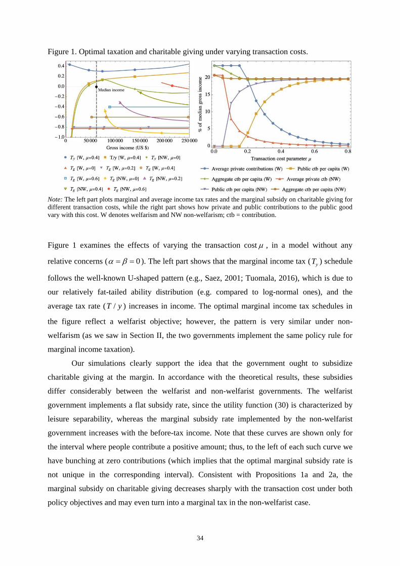
34

Figure 1. Optimal taxation and charitable giving under varying transaction costs.

Note: The left part plots marginal and average income tax rates and the marginal subsidy on charitable giving for

different transaction costs, while the right part shows how private and public contributions to the public good

vary with this cost. W denotes welfarism and NW non-welfarism; ctb = contribution.

Figure 1 examines the effects of varying the transaction cost , in a model without any

relative concerns ( 0 ). The left part shows that the marginal income tax (yT ) schedule

follows the well-known U-shaped pattern (e.g., Saez, 2001; Tuomala, 2016), which is due to

our relatively fat-tailed ability distribution (e.g. compared to log-normal ones), and the

average tax rate ( /T y ) increases in income. The optimal marginal income tax schedules in

the figure reflect a welfarist objective; however, the pattern is very similar under non-

welfarism (as we saw in Section II, the two governments implement the same policy rule for

marginal income taxation).

Our simulations clearly support the idea that the government ought to subsidize

charitable giving at the margin. In accordance with the theoretical results, these subsidies

differ considerably between the welfarist and non-welfarist governments. The welfarist

government implements a flat subsidy rate, since the utility function (30) is characterized by

leisure separability, whereas the marginal subsidy rate implemented by the non-welfarist

government increases with the before-tax income. Note that these curves are shown only for

the interval where people contribute a positive amount; thus, to the left of each such curve we

have bunching at zero contributions (which implies that the optimal marginal subsidy rate is

not unique in the corresponding interval). Consistent with Propositions 1a and 2a, the

marginal subsidy on charitable giving decreases sharply with the transaction cost under both

policy objectives and may even turn into a marginal tax in the non-welfarist case.

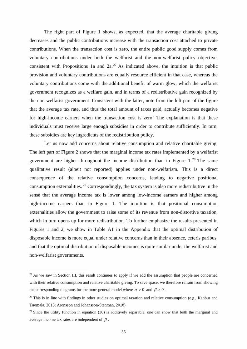
35

The right part of Figure 1 shows, as expected, that the average charitable giving

decreases and the public contributions increase with the transaction cost attached to private

contributions. When the transaction cost is zero, the entire public good supply comes from

voluntary contributions under both the welfarist and the non-welfarist policy objective,

consistent with Propositions 1a and 2a.27 As indicated above, the intuition is that public

provision and voluntary contributions are equally resource efficient in that case, whereas the

voluntary contributions come with the additional benefit of warm glow, which the welfarist

government recognizes as a welfare gain, and in terms of a redistributive gain recognized by

the non-welfarist government. Consistent with the latter, note from the left part of the figure

that the average tax rate, and thus the total amount of taxes paid, actually becomes negative

for high-income earners when the transaction cost is zero! The explanation is that these

individuals must receive large enough subsidies in order to contribute sufficiently. In turn,

these subsidies are key ingredients of the redistribution policy.

Let us now add concerns about relative consumption and relative charitable giving.

The left part of Figure 2 shows that the marginal income tax rates implemented by a welfarist

government are higher throughout the income distribution than in Figure 1.28 The same

qualitative result (albeit not reported) applies under non-welfarism. This is a direct

consequence of the relative consumption concerns, leading to negative positional

consumption externalities. 29 Correspondingly, the tax system is also more redistributive in the

sense that the average income tax is lower among low-income earners and higher among

high-income earners than in Figure 1. The intuition is that positional consumption

externalities allow the government to raise some of its revenue from non-distortive taxation,

which in turn opens up for more redistribution. To further emphasize the results presented in

Figures 1 and 2, we show in Table A1 in the Appendix that the optimal distribution of

disposable income is more equal under relative concerns than in their absence, ceteris paribus,

and that the optimal distribution of disposable incomes is quite similar under the welfarist and

non-welfarist governments.

27 As we saw in Section III, this result continues to apply if we add the assumption that people are concerned

with their relative consumption and relative charitable giving. To save space, we therefore refrain from showing

the corresponding diagrams for the more general model where 0 and 0 .

28 This is in line with findings in other studies on optimal taxation and relative consumption (e.g., Kanbur and

Tuomala, 2013; Aronsson and Johansson-Stenman, 2018).

29 Since the utility function in equation (30) is additively separable, one can show that both the marginal and

average income tax rates are independent of .

36

Figure 2. Tax policy, charitable giving, and variation in .

Note: The left part plots marginal and average income tax rate and the marginal subsidy on charitable giving,

while the right part shows how the private and public contributions to the public good vary with the degree of

charitable positionality, . W denotes welfarism and NW non-welfarism; ctb = contribution.

As expected from Proposition 3a, the left part of Figure 2 also shows that the marginal tax

treatment of charitable giving differs substantially between the two policy objectives. The

marginal subsidy is again constant among givers under welfarism and increases with the

before-tax income under non-welfarism, although the levels of the marginal subsidies differ

from those in Figure 1. The marginal subsidy on charitable giving decreases with the degree

of gifts positionality, , under welfarism. In the non-welfarist case, the marginal subsidy is

much less sensitive to (and even increases with) . This is because very few individuals

contribute to charity under non-welfarism in our model. As explained in Section III, this

means that non becomes large, which reduces the social cost of the positional gifts

externality. The right part of Figure 2 shows, correspondingly, that the average charitable

giving decreases with , and that the governmental contribution increases with , under

welfarism. These relationships are absent under a non-welfarist objective.

Figure 3 shows how the marginal tax treatment of charitable giving as well as the

private and public contributions to the public good vary with the degree of consumption

positionality, , when all other parameters reflect the numerical reference scenario. The left

part illustrates how the optimal marginal subsidy schedule for charitable giving varies with

.30 In accordance with the policy rules for gT presented in Proposition 3a, we can see that a

30 Again for simplicity, we only present one curve each for the marginal and average income tax rates

(corresponding to the numerical reference scenario where 0.2 and 0.25 ), although these rates will now

vary considerably with , as shown by comparing Figures 1 and 2.

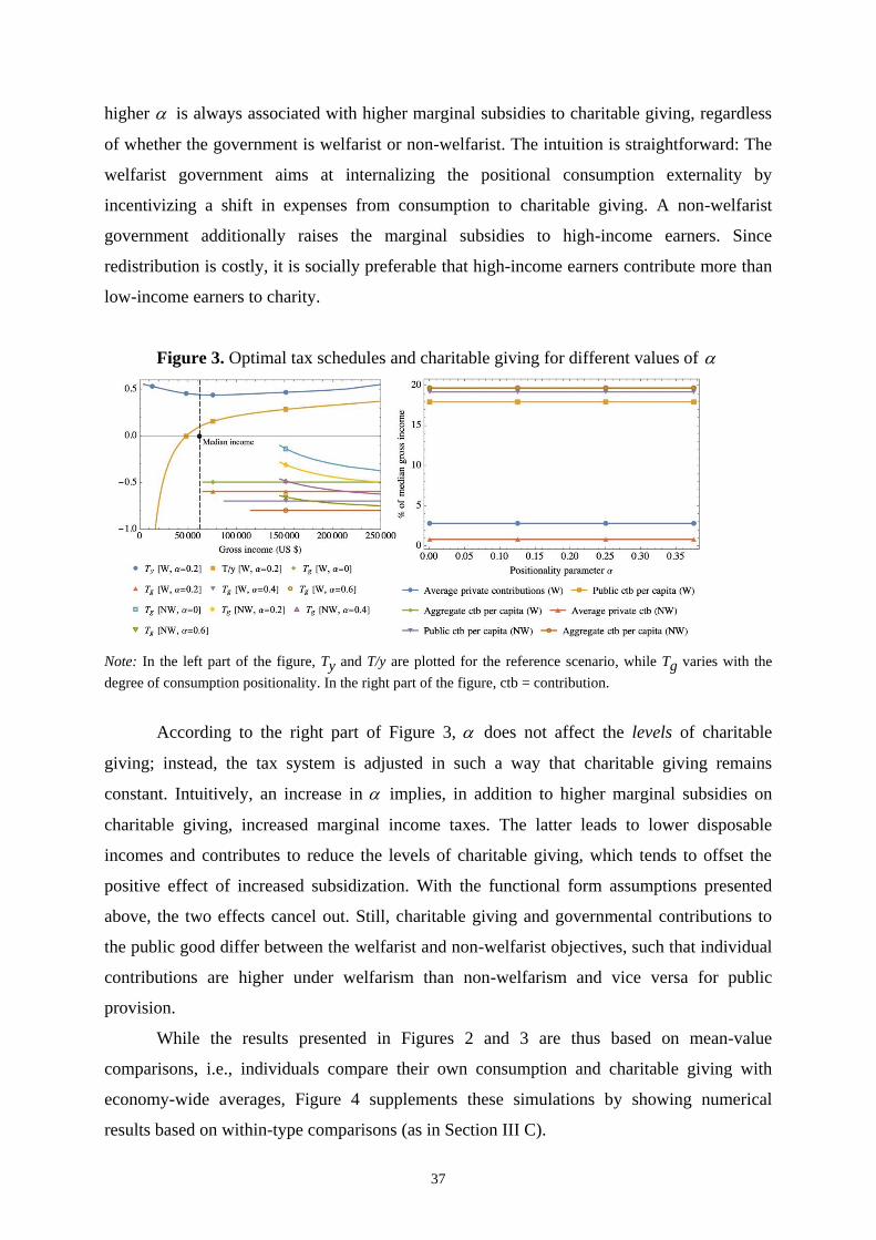
37

higher is always associated with higher marginal subsidies to charitable giving, regardless

of whether the government is welfarist or non-welfarist. The intuition is straightforward: The

welfarist government aims at internalizing the positional consumption externality by

incentivizing a shift in expenses from consumption to charitable giving. A non-welfarist

government additionally raises the marginal subsidies to high-income earners. Since

redistribution is costly, it is socially preferable that high-income earners contribute more than

low-income earners to charity.

Figure 3. Optimal tax schedules and charitable giving for different values of

Note: In the left part of the figure, Ty and T/y are plotted for the reference scenario, while Tg varies with the

degree of consumption positionality. In the right part of the figure, ctb = contribution.

According to the right part of Figure 3, does not affect the levels of charitable

giving; instead, the tax system is adjusted in such a way that charitable giving remains

constant. Intuitively, an increase in implies, in addition to higher marginal subsidies on

charitable giving, increased marginal income taxes. The latter leads to lower disposable

incomes and contributes to reduce the levels of charitable giving, which tends to offset the

positive effect of increased subsidization. With the functional form assumptions presented

above, the two effects cancel out. Still, charitable giving and governmental contributions to

the public good differ between the welfarist and non-welfarist objectives, such that individual

contributions are higher under welfarism than non-welfarism and vice versa for public

provision.

While the results presented in Figures 2 and 3 are thus based on mean-value

comparisons, i.e., individuals compare their own consumption and charitable giving with

economy-wide averages, Figure 4 supplements these simulations by showing numerical

results based on within-type comparisons (as in Section III C).

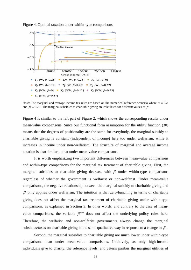
38

Figure 4. Optimal taxation under within-type comparisons

Note: The marginal and average income tax rates are based on the numerical reference scenario where 0.2

and 0.25 . The marginal subsidies to charitable giving are calculated for different values of .

Figure 4 is similar to the left part of Figure 2, which shows the corresponding results under

mean-value comparisons. Since our functional form assumption for the utility function (30)

means that the degrees of positionality are the same for everybody, the marginal subsidy to

charitable giving is constant (independent of income) here too under welfarism, while it

increases in income under non-welfarism. The structure of marginal and average income

taxation is also similar to that under mean-value comparisons.

It is worth emphasizing two important differences between mean-value comparisons

and within-type comparisons for the marginal tax treatment of charitable giving. First, the

marginal subsidies to charitable giving decrease with under within-type comparisons

regardless of whether the government is welfarist or non-welfarist. Under mean-value

comparisons, the negative relationship between the marginal subsidy to charitable giving and

only applies under welfarism. The intuition is that zero-bunching in terms of charitable

giving does not affect the marginal tax treatment of charitable giving under within-type

comparisons, as explained in Section 3. In other words, and contrary to the case of mean-

value comparisons, the variable non does not affect the underlying policy rules here.

Therefore, the welfarist and non-welfarist governments always change the marginal

subsidies/taxes on charitable giving in the same qualitative way in response to a change in .

Second, the marginal subsidies to charitable giving are much lower under within-type

comparisons than under mean-value comparisons. Intuitively, as only high-income

individuals give to charity, the reference levels, and ceteris paribus the marginal utilities of

39

giving, are higher under within-type than mean-value comparisons. Consequently, to reach a

given level of the public good, we need less subsidization under within-type comparisons.

VI. Conclusion

Let us return to the question posed initially: What is the optimal tax treatment of charitable

giving? While the answer is, naturally, complex, we would like to emphasize eight key results.

1) For a welfarist government, zero transaction costs and leisure separability, regardless of

relative concerns, together imply that charitable giving should be subsidized to an extent that

completely crowds out governmental contribution to the public good. 2) The same result

holds for a non-welfarist government that does not value the warm glow of giving. 3) The

optimal marginal subsidy to charitable giving decreases strongly with the size of the

transaction costs. 4) When these costs are sufficiently high, the marginal subsidy decreases

with the degree of charitable positionality, and the marginal subsidy is much lower for a non-

welfarist than for a welfarist government. 5) A welfarist government would implement a flat

rate marginal subsidy on charitable giving under leisure separability, regardless of whether

individuals are concerned with their relative consumption and relative charitable giving.

Conditions are presented for when the marginal subsidy increases or decreases with income

for a non-welfarist government. 6) Zero bunching in terms of charitable giving implies higher

marginal subsidies for the contributors, ceteris paribus. 7) In the general case where the utility

functions are non-separable, we also show how public good provision and the marginal

subsidies/taxes on charitable giving supplement the income tax for purposes of redistribution,

and how the redistributive roles of these two instruments depend on the income tax wedge. 8)

Stronger concerns for relative charitable giving tend to support lower marginal subsidies,

whereas concerns for relative consumption work in the other direction. These, and several

other, qualitative insights continue to hold in our dual screening setting.

Appendix

Proof of Propositions 3 (Propositions 1 and 2 follow as special cases)

We start by proving Proposition 3b for the welfarist case. In the optimal control problems, we

treat utility, wu , as a state variable, while wl , wg , GovG , c , and g are control variables.

Consumption, wc , is defined by the inverse of the function ( )u in (17), i.e.,

( , , , , , ; )w w w wc h l g G c g u w . The Lagrangean becomes

40

0 0

0

0 0 0

( ) ( ) ( , , , , , ; ) ( )

( ( , , , , , ; ), , , ))

( , , , , , ; ) ( ) ( )

Gov

w w w w w w

l w w w w w ww w w

Gov

w w w w w w

L u f w dw wl h l g G g c u w g f w dw G

u h l g G g c u w l g G lu dw

w

c h l g G g c u w f w dw g g f w dw g dw G

. (A1)

To avoid clutter, we suppress the type indicator w except in integral expressions. By using

,/l l c l ch u u MRS and ,/G G c G ch u u MRS , the social first-order conditions for l

and GovG , respectively, if 0GovG , can be written as

,

, ,1 0( )

c l c lc

l c l l c

u MRSw MRS MRS

f w w

(A2)

( )

,( ) ( )

,

0 0

11 ( ) 1

w

G cw w Gc

G c w c l

MRSMRS f w dw u dw

w

. (A3)

We can derive an expression for / from the social first-order condition for c . By using

,/c c c c ch u u MRS , the social first-order condition for c can be written as follows:

( )

,( ) ( ) ( )

, ,

0 0 0

1( ) 1 ( ) 0

w

c cw w www c c c c c

MRS lu dw MRS f w dw MRS f w dw

l w

. (A4)

Since ,c cMRS ,

0( )w f w dw

, and , / /c cMRS l l , (A4) implies

( )

0

1 1

1 1 1

w d

wl dwl w

. (A5)

Substitute (A5) into (A2) and (A3) and use the private first-order condition ,l c yw MRS wT .

Finally, use ( ) / ( )w

w w c wB C u wf w and rearrange to obtain (i) and the first part of (ii) in

Proposition 3b.

By using ,/g g c g ch u u MRS and

, ,/g g c g c g ch u u MRS MRS , the social

first-order conditions for g and g , respectively, can be written as follows if 0GovG :

,

, 1( ) ( )

g ccg c

MRSu lMRS

f w l w f w

(A6)

,( ) ( )

, ,

0 0

11 ( )

w

g cw w ww ww c g c w w g c

MRS lu MRS dw MRS f w dw

l l w

. (A7)

Substituting (A6) into (A7) gives

41

( )

0 0

1 1 1 1

1 1 1 1

d nonw w w

w g w w

lu dw dw

l w

. (A8)

Substitute (A8) into (A6) and use the private first-order condition , 1g c gMRS T . Finally,

write the first term on the right-hand side of (A6) in elasticity form and

use ( ) / ( )w

w w c wB C u wf w . This gives the policy rule for gT in Proposition 3b. If 0GovG ,

the derivation procedure is the same, except that (A3) does not hold and 0(1 )S will be

added to the right-hand side of (A6), where 0S is given by

( )

,0

0 0

1 ( )1

Gov

w

G c

G

MRSS f w dw

.

Proposition 3a follows as the special case where the utility functions are leisure separable,

which implies ( ) ( ) 0Gc gc d d

l w l w for all w. The corresponding policy rules in

Proposition 1 follow as special cases where 0w w for all w, in which 0 .

In order to show (iv) of Proposition 3b in the welfarist case, note that under zero

transaction costs the social first-order conditions for wg and GovG can be written as

0( ) ( )

, ( ) ,

1 1 1: 0

1 1 1 1 1

non dw gc w

w g c l w w w g cd d d

Sg MRS B C MRS w

( ) 0

,

0

1: ( ) 1 0

1

dGov w Gc

G c l w wG MRS B C f w dw S

,

where strict equality holds for individuals who contribute to the public good ( 0wg ). Also,

recall that 0 0S if 0GovG and 0 0S if 0GovG . Assume now that we have an interior

solution in the sense that both the government and some individuals contribute. This means

that 0 0S . However, the social first-order conditions for wg are not satisfied in this case.

Instead, if d non , 1d , and

( ) 0gc

l w , we obtain

( ) ( )

, ( ) ,

1 10

1 1 1

non dw gc w

g c l w w w g cd dMRS B C MRS

,

since all three terms on the left-hand side are positive. Thus, the only way of satisfying the

social first-order conditions simultaneously is to choose 0GovG , so 0 0S . It is also

obvious that we do not need all three terms to be positive for this result to hold; it suffices that

their sum is positive.

Result (iv) of Proposition 3a, i.e., under leisure separability, follows as the special case

where ( ) ( ) 0Gc gc d d

l w l w for all w. Again the corresponding results in Proposition 1

42

follow as special cases where 0w w for all w, in which 0 .

We will next prove Proposition 3b for the non-welfarist case, where the Lagrangean

can be written as follows:

0 0

0

0 0

0

( ) ( ) ( , , , , , ; ) ( )

( ( , , , , , ; ), , , ))

( , , , , , ; ) ( ) ( )

( ( ,

n Gov

w w w w w w

l w w w w w ww w w

w w w w

w w w w

L u f w dw wl h l g G g c u w g f w dw G

u h l g G g c u w l g G lu dw

w

c h l g G g c u w f w dw g g f w dw

g dw h l g

0

, , , , ; ), , , ; ) n Gov

w w w wG g c u w l c G w u dw G

. (A9)

There are two state variables here, u and nu , whereas the control variables are the same as

above. Note that 0c l lh , 0c G Gh , and 0c c ch , which means that the social

first-order conditions for l , GovG , and c coincide with equations (A2), (A3), and (A4),

respectively. If 0GovG , the social first-order conditions for g and g , i.e., analogues of

equations (A6) and (A7), can now be written as

,

, ,

'( )1

( ) ( )

g cc cg c g c

MRSu ulMRS MRS

f w l w f w

(A10)

,( ) ( )

, ,

0 0

( ) ( )

,

0

11 ( )

1'( ) ( )

w

g cw w ww ww c g c w w g c

w w

w c w g c

MRS lu MRS dw MRS f w dw

l l w

u f w MRS dw

. (A11)

Combining them gives equation (A8) above. Finally, substituting (A8) into (A10) and using

the private first-order condition for charitable giving, we can derive the non-welfarist policy

rule for gT in Proposition 3b. Again, the derivation is analogous if 0GovG at the social

optimum. Proposition 3a follows as the special case where the utility functions are leisure

separable. The corresponding policy rules in Proposition 2 follow as special cases where

0w w for all w, in which 0 .

To show (iv) in the non-welfarist case, note that zero transaction cost implies that the

social first-order conditions for wg and GovG can be written as

0( ) ( )

, ( ) ,

1 1 1 1: 1 0

1 1 1 1 1 1

non dw gc w

w g c w l w w w g cd d d d

Sg MRS B C MRS w

,

43

( ) 0

,

0

1: ( ) 1 0

1

dGov w Gc

G c l w wG MRS B C f w dw S

,

Based on the same reasoning as in the welfarist case, if non d and 1d , we must have

0GovG (such that 0 0S ) for these conditions to hold simultaneously. The corresponding

policy rules in Proposition 2a follow as special cases where 0w w for all w, in which

0 .

Proof of Proposition 4

To shorten the notation, let ( , )w b represent type in two-dimensional space, and let

( ) ( , )f f w b denote the corresponding density function such that

0 0

( ) ( , ) 1f d f w b db dw

.

In a way similar to the proof of Propositions 3 above, we treat utility, u , as a state variable,

while l , g , GovG , c , and g are control variables. Consumption, c , is defined by the

inverse of the function ( )u in equation (27), i.e., ( , , , , , ; )c h l g G c g u .

With a welfarist government, the Lagrangean can be written as follows:

( )( )

( ) ( )

( , , , , , ; ) ( )

( )

( , , , , , ; ) ( )

( )

Gov

w b w blc

Gov

L u f d

w l h l g c g G u g f d G

l uu u d

w

c h l g G c g u f d

g g f d g d G

. (A12)

Under non-welfarism, equation (33) is added to the set of constraints, and nu will be used as

an additional state variable. Therefore, the Lagrangean is given by

( )( )

( ) ( )

( , , , , , ; ) ( )

( )

( , , , , , ; ) ( ) ( )

( ( , , , , , ; ), , , ; )

n

Gov

w b w blc

n

L u f d

w l h l g c g G u g f d G

l uu u d

w

c h l g G c g u f d g g f d

h l g G c g u l c G u d g d

GovG

. (A13)

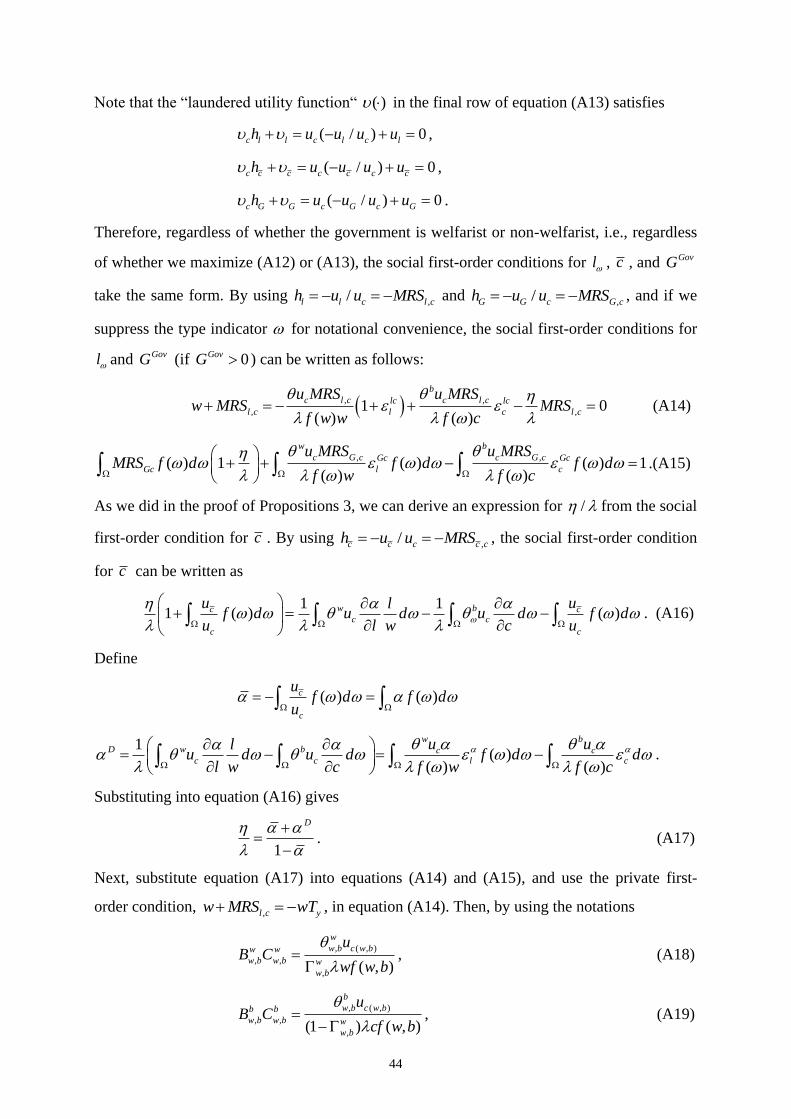
44

Note that the “laundered utility function“ ( ) in the final row of equation (A13) satisfies

( / ) 0c l l c l c lh u u u u ,

( / ) 0c c c c c c ch u u u u ,

( / ) 0c G G c G c Gh u u u u .

Therefore, regardless of whether the government is welfarist or non-welfarist, i.e., regardless

of whether we maximize (A12) or (A13), the social first-order conditions for l , c , and GovG

take the same form. By using ,/l l c l ch u u MRS and

,/G G c G ch u u MRS , and if we

suppress the type indicator for notational convenience, the social first-order conditions for

l and GovG (if 0GovG ) can be written as follows:

, ,

, ,1 0( ) ( )

b

c l c c l clc lc

l c l c l c

u MRS u MRSw MRS MRS

f w w f c

(A14)

, ,( ) 1 ( ) ( ) 1

( ) ( )

w b

c G c c G cGc Gc

Gc l c

u MRS u MRSMRS f d f d f d

f w f c

.(A15)

As we did in the proof of Propositions 3, we can derive an expression for / from the social

first-order condition for c . By using ,/c c c c ch u u MRS , the social first-order condition

for c can be written as

1 1

1 ( ) ( )w bc cc c

c c

u ulf d u d u d f d

u l w c u

. (A16)

Define

( ) ( )c

c

uf d f d

u

1( )

( ) ( )

w bD w b c c

c c l c

u ulu d u d f d d

l w c f w f c

.

Substituting into equation (A16) gives

1

D

. (A17)

Next, substitute equation (A17) into equations (A14) and (A15), and use the private first-

order condition, ,l c yw MRS wT , in equation (A14). Then, by using the notations

, ( , )

, ,

, ( , )

w

w b c w bw w

w b w b w

w b

uB C

wf w b

, (A18)

, ( , )

, ,

,(1 ) ( , )

b

w b c w bb b

w b w b w

w b

uB C

cf w b

, (A19)

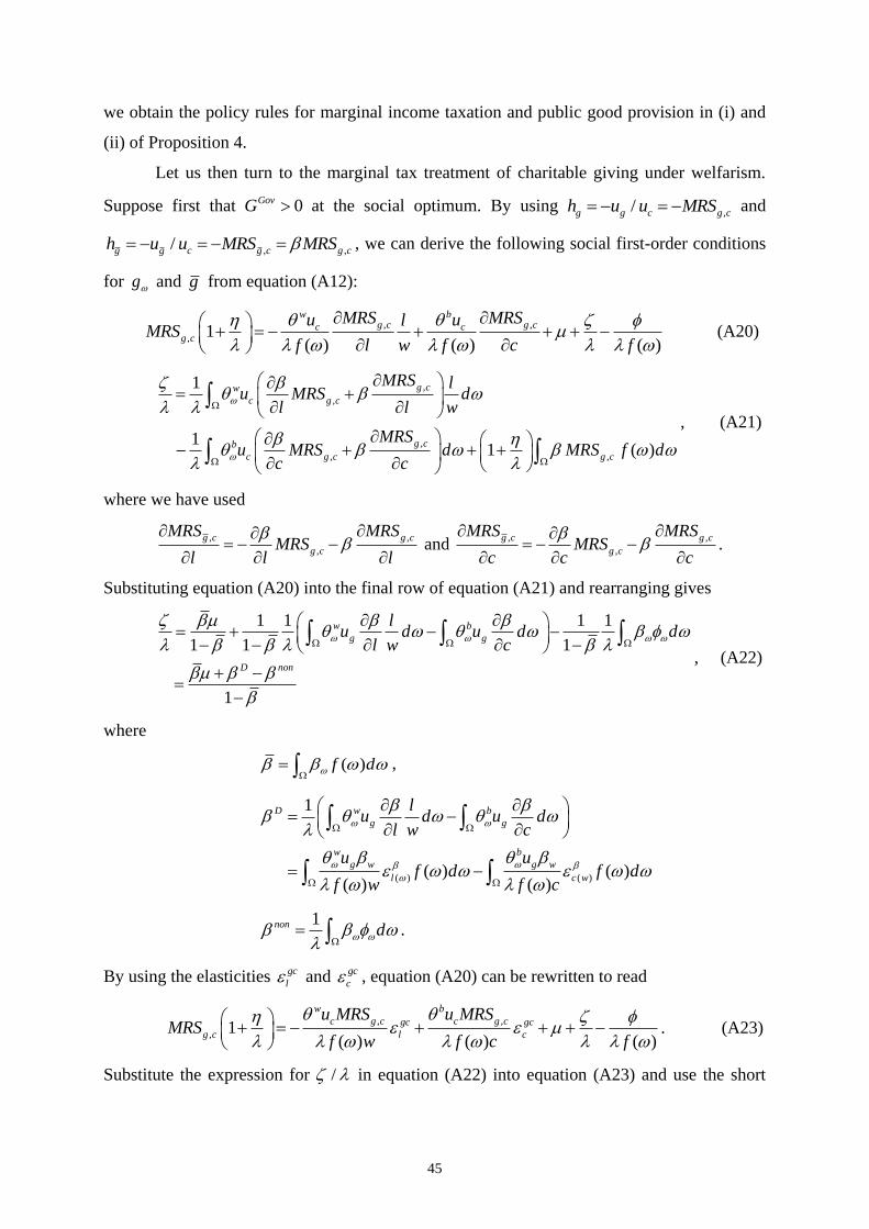
45

we obtain the policy rules for marginal income taxation and public good provision in (i) and

(ii) of Proposition 4.

Let us then turn to the marginal tax treatment of charitable giving under welfarism.

Suppose first that 0GovG at the social optimum. By using ,/g g c g ch u u MRS and

, ,/g g c g c g ch u u MRS MRS , we can derive the following social first-order conditions

for g and g from equation (A12):

, ,

, 1( ) ( ) ( )

w bg c g cc c

g c

MRS MRSu ulMRS

f l w f c f

(A20)

,

,

,

, ,

1

11 ( )

g cw

c g c

g cb

c g c g c

MRS lu MRS d

l l w

MRSu MRS d MRS f d

c c

, (A21)

where we have used

, ,

,

g c g c

g c

MRS MRSMRS

l l l

and

, ,

,

g c g c

g c

MRS MRSMRS

c c c

.

Substituting equation (A20) into the final row of equation (A21) and rearranging gives

1 1 1 1

1 1 1

1

w b

g g

D non

lu d u d d

l w c

, (A22)

where

( )f d

,

( ) ( )

1

( ) ( )( ) ( )

D w b

g g

w b

g w g w

l c w

lu d u d

l w c

u uf d f d

f w f c

1non d

.

By using the elasticities gc

l and gc

c , equation (A20) can be rewritten to read

, ,

, 1( ) ( ) ( )

w b

c g c c g cgc gc

g c l c

u MRS u MRSMRS

f w f c f

. (A23)

Substitute the expression for / in equation (A22) into equation (A23) and use the short

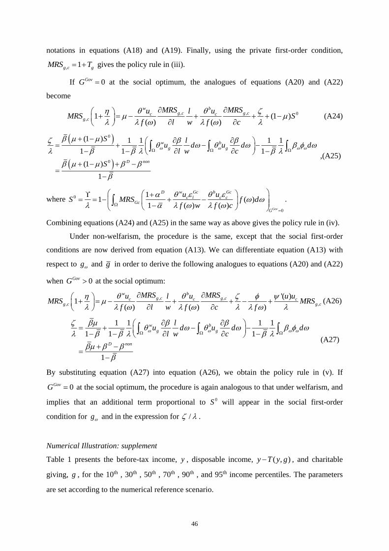
46

notations in equations (A18) and (A19). Finally, using the private first-order condition,

, 1g c gMRS T gives the policy rule in (iii).

If 0GovG at the social optimum, the analogues of equations (A20) and (A22)

become

, , 0

, 1 (1 )( ) ( )

w bg c g cc c

g c

MRS MRSu ulMRS S

f l w f c

(A24)

0

0

(1 ) 1 1 1 1

1 1 1

(1 )

1

w b

g g

D non

S lu d u d d

l w c

S

,(A25)

where 0

0

11 ( )

1 ( ) ( )Gov

w Gc b GcD

c l c cGc

G

u uS MRS f d

f w f c

.

Combining equations (A24) and (A25) in the same way as above gives the policy rule in (iv).

Under non-welfarism, the procedure is the same, except that the social first-order

conditions are now derived from equation (A13). We can differentiate equation (A13) with

respect to g and g in order to derive the following analogues to equations (A20) and (A22)

when 0GovG at the social optimum:

, ,

, ,

'( )1

( ) ( ) )

w bg c g cc c c

g c g c

MRS MRSu u u ulMRS MRS

f l w f c f

(A26)

1 1 1 1

1 1 1

1

w b

g g

D non

lu d u d d

l w c

(A27)

By substituting equation (A27) into equation (A26), we obtain the policy rule in (v). If

0GovG at the social optimum, the procedure is again analogous to that under welfarism, and

implies that an additional term proportional to 0S will appear in the social first-order

condition for g and in the expression for / .

Numerical Illustration: supplement

Table 1 presents the before-tax income, y , disposable income, ( , )y T y g , and charitable

giving, g , for the 10th , 30th , 50th , 70th , 90th , and 95th income percentiles. The parameters

are set according to the numerical reference scenario.

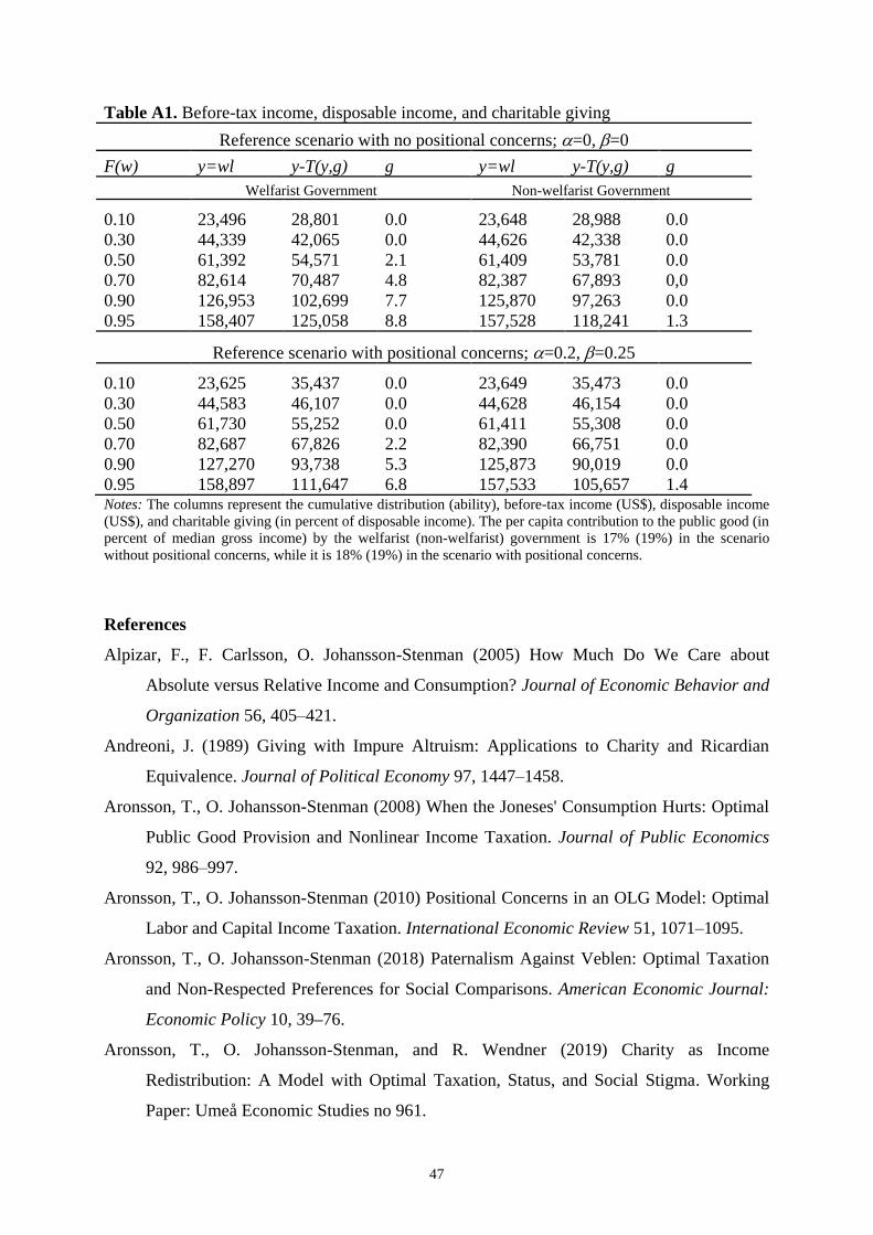
47

Table A1. Before-tax income, disposable income, and charitable giving

Reference scenario with no positional concerns; =0, =0

F(w) y=wl y-T(y,g) g y=wl y-T(y,g) g

Welfarist Government Non-welfarist Government

0.10 23,496 28,801 0.0 23,648 28,988 0.0

0.30 44,339 42,065 0.0 44,626 42,338 0.0

0.50 61,392 54,571 2.1 61,409 53,781 0.0

0.70 82,614 70,487 4.8 82,387 67,893 0,0

0.90 126,953 102,699 7.7 125,870 97,263 0.0

0.95 158,407 125,058 8.8 157,528 118,241 1.3

Reference scenario with positional concerns; =0.2, =0.25

0.10 23,625 35,437 0.0 23,649 35,473 0.0

0.30 44,583 46,107 0.0 44,628 46,154 0.0

0.50 61,730 55,252 0.0 61,411 55,308 0.0

0.70 82,687 67,826 2.2 82,390 66,751 0.0

0.90 127,270 93,738 5.3 125,873 90,019 0.0

0.95 158,897 111,647 6.8 157,533 105,657 1.4 Notes: The columns represent the cumulative distribution (ability), before-tax income (US$), disposable income

(US$), and charitable giving (in percent of disposable income). The per capita contribution to the public good (in

percent of median gross income) by the welfarist (non-welfarist) government is 17% (19%) in the scenario

without positional concerns, while it is 18% (19%) in the scenario with positional concerns.

References

Alpizar, F., F. Carlsson, O. Johansson-Stenman (2005) How Much Do We Care about

Absolute versus Relative Income and Consumption? Journal of Economic Behavior and

Organization 56, 405–421.

Andreoni, J. (1989) Giving with Impure Altruism: Applications to Charity and Ricardian

Equivalence. Journal of Political Economy 97, 1447–1458.

Aronsson, T., O. Johansson-Stenman (2008) When the Joneses' Consumption Hurts: Optimal

Public Good Provision and Nonlinear Income Taxation. Journal of Public Economics

92, 986–997.

Aronsson, T., O. Johansson-Stenman (2010) Positional Concerns in an OLG Model: Optimal

Labor and Capital Income Taxation. International Economic Review 51, 1071–1095.

Aronsson, T., O. Johansson-Stenman (2018) Paternalism Against Veblen: Optimal Taxation

and Non-Respected Preferences for Social Comparisons. American Economic Journal:

Economic Policy 10, 39–76.

Aronsson, T., O. Johansson-Stenman, and R. Wendner (2019) Charity as Income

Redistribution: A Model with Optimal Taxation, Status, and Social Stigma. Working

Paper: Umeå Economic Studies no 961.

48

Atkinson, A.B. (1976) The Income Tax Treatment of Charitable Contributions. In: Grieson,

R. (Ed.), Public and Urban Economics: Essays in the Honor of William S. Vickrey. D.C.

Heath, New York.

Atkinson, A. B., J. E. Stiglitz (1976) The Design of Tax Structure: Direct versus Indirect

Taxation. Journal of Public Economics 6, 55–75.

Blanchflower, D.G., A.J. Oswald (2004) Well-Being Over Time in Britain and the USA.

Journal of Public Economics 88, 1359–1386.

Bergstrom, T., L. Blume, H. Varian (1986) On the Private Provision of Public Goods. Journal

of Public Economics 29, 25–49.

Blumkin, T., E. Sadka (2007) A case for taxing charitable donations. Journal of Public

Economics 91, 1555–1564.

Boadway, R., M. Keen (1993) Public Goods, Self-Selection and Optimal Income Taxation.

International Economic Review 34, 463–478.

Boskin, M.J., E. Sheshinski (1978) Individual Welfare Depends Upon Relative Income.

Quarterly Journal of Economics 92, 589–601.

Carlsson, F., O. Johansson-Stenman, P. Martinsson (2007) Do You Enjoy Having More Than

Others? Survey Evidence of Positional Goods. Economica 74, 586–598.

Christiansen, V. (1981) Evaluation of Public Projects under Optimal Taxation. Review of

Economic Studies 48, 447–457.

Clark, A., C. Senik (2010) Who Compares to Whom? The Anatomy of Income Comparisons

in Europe. Economic Journal 120, 573–594.

Cremer, H., P. Pestieau, J-C. Rochet (2001) Direct Versus Indirect Taxation: The Design of

the Tax Structure Revisited. International Economic Review 42, 781–800.

DellaVigna, S., J. List, U. Malmendier (2012) Testing for Altruism and Social Pressure in

Charitable Giving. Quarterly Journal of Economics 127, 1–56.

Diamond, P. (1980) Income Taxation with Fixed Hours of Work. Journal of Public

Economics 13, 101–110.

Diamond, P. (1998) Optimal Income Taxation: An Example with a U-Shaped Pattern of

Optimal Marginal Tax Rates. American Economic Review 88, 83–95.

Diamond, P. (2006) Optimal Tax Treatment of Private Contributions for Public Goods with

and Without Warm-Glow Preferences. Journal of Public Economics 90, 897–919.

Dupor, B., W.F. Liu (2003) Jealousy and Overconsumption. American Economic Review 93,

423–428.

49

Easterlin, R.A. (2001) Income and Happiness: Towards a Unified Theory. Economic Journal

111, 465–484.

Eckerstorfer, P., R. Wendner (2013) Asymmetric and Non-Atmospheric Consumption

Externalities, and Efficient Consumption Taxation. Journal of Public Economics 106,

42–56.

Fack, G., C. Laindais, eds., (2012) Charitable Giving and Tax Policy: A Historical and

Comparative Perspective. Conference Volume, CEPR/CEPREMAP Conference on

Altruism and Charitable Giving held in May 2012, Paris School of Economics.

Feldstein, M. (1980) A Contribution to the Theory of Tax Expenditures: The Case of

Charitable Giving. In: Aaron, H. J., and M. J. Boskin (Eds.), The Economics of

Taxation, Essays in Honor of Joseph Peckman, 99–122. Brookings Institution,

Washington, D.C.

Ferrer-i-Carbonell, A. (2005) Income and Well-being: An Empirical Analysis of the

Comparison Income Effect. Journal Public Economics 89, 997–1019.

Giving USA (2020), The Annual Report on Philanthropy for the Year 2019, a publication of

Giving USA Foundation, 2020, Indiana University Lilly Family School of Philanthropy.

Glazer, A., K. Konrad (1996) A Signaling Explanation for Charity. American Economic

Review 86, 1019–1028.

Golosov, M., A. Tsyvinski, N. Werquin (2014) Dynamic Tax Reforms. NBER Working

Papers 20 780.

Harbaugh, W. (1998) The Prestige Motive for Making Charitable Transfers. American

Economic Review 88, 277–282.

Harsanyi, J. (1982) Morality and the Theory of Rational Behavior. In Utilitarianism and

Beyond, edited by Sen, A. and Williams, B. Cambridge: Cambridge University Press.

Jacobs, B., R. Boadway (2014) Optimal Linear Commodity Taxation under Optimal Non-

linear Income Taxation. Journal of Public Economics 117, 201–210.

Johansson-Stenman, O., F. Carlsson, D. Daruvala (2002) Measuring Future Grandparents'

Preferences for Equality and Relative Standing. Economic Journal 112, 362–383.

Kanbur, R., M. Tuomala (2013) Relativity, Inequality and Optimal Nonlinear Income

Taxation. International Economic Review 54, 1199–1217.

Kaplow, L. (1995) A note on subsidizing gifts. Journal of Public Economics 58, 469–477.

Kaplow, L. (1998) Tax Policy and Gifts. American Economic Review, Papers and

Proceedings 88, 283–288.

50

Kaplow, L., S. Shavell (2001) Any Non-welfarist Method of Policy Assessment Violates the

Pareto Principle. Journal of Political Economy 109, 281–286.

Kleven, H. J., C. T. Kreiner, E. Saez (2009) The Optimal Income Taxation of Couples.

Econometrica 77, 537–560.

Lehmann, E., S. Renes, K. Spiritus, F. Zoutman (2020) Optimal Taxation with Multiple

Incomes and Types. Mimeo.

Ljungqvist, L., H. Uhlig (2000) Tax Policy and Aggregate Demand Management Under

Catching Up with the Joneses. American Economic Review 90, 356–366.

Mirrlees, J. (1971) An Exploration in the Theory of Optimal Income Taxation. Review of

Economic Studies 38, 175–208.

Mirrlees, J. (1986) The Theory of Optimal Taxation. In K. J. Arrow and M.D. Intriligator,

eds., Handbook of Mathematical Economics, Vol. 3, Elsevier, chapter 24, 1197–1249.

Oswald, A. (1983) Altruism, Jealousy and the Theory of Optimal Non-Linear Taxation.

Journal of Public Economics 20, 77–87.

Renes, R., F. Zoutman (2017) As Easy as ABC? Multidimensional Screening in Public

Finance. CESifo Working Paper No. 6301.

Runciman, W.G. (1966) Relative Deprivation and Social Justice. London: Routledge and

Kegan Paul.

Saez, E. (2001) Using Elasticities to Derive Optimal Income Tax Rates. Review of Economic

Studies 68, 205–229.

Saez, E. (2002) The Desirability of Commodity Taxation under Non-Linear Income Taxation

and Heterogeneous Tastes. Journal of Public Economics 83, 217–230.

Saez, E., (2004) The Optimal Treatment of Tax Expenditures. Journal of Public Economics

88, 2657–2684.

Solnick, S., D. Hemenway (2005) Are Positional Concerns Stronger in Some Domains than in

Others? American Economic Review, Papers and Proceedings 45, 147–151.

Tuomala, M. (2016) Optimal Redistributive Taxation. Oxford: Oxford University Press.

Veblen, T. (1899) The Theory of the Leisure Class: An Economic Study in the Evolution of

Institutions. New York: Macmillan.

Warr, P. (1982). Pareto Optimal Redistribution and Private Charity. Journal of Public

Economics 19, 131–138.

Wendner, R., L.H. Goulder (2008) Status Effects, Public Goods Provision, and the Excess

Burden. Journal of Public Economics 92, 1968–1985.