CHARGED HADRON PRODUCTION IN E+ E- ANNIHILATION AT S**(1…

SLAC-R-713

CHARGED HADRON PRODUCTION IN E+ E- ANNIHILATION AT S**(1/2) = 29-GEV*

Zachary Wolf

Stanford Linear Accelerator Center Stanford University Stanford, CA 94309

SLAC-Report-713 September 1987

Prepared for the Department of Energy under contract number DE-AC03-76SF00515

Printed in the United States of America. Available from the National Technical Information Service, U.S. Department of Commerce, 5285 Port Royal Road, Springfield, VA 22161.

* Ph.D. thesis, Lawrence Berkeley Laboratory, Berkeley, CA 94720

LBL-23738

Charged Hadron Production In e+e- Annihilation At fi = 29 GeV

BY Zachary Wolf Ph.D. Thesis

September 2, 1987

Lawrence Berkeley Laboratory University of California

Berkeley, CA 94720

Abstract

Data from the Time Projection Chamber at the SLAC storage ring PEP have been used to study the inclusive production of charged hadrons. Particles were identified by simultaneous dE/dz and momentum measurements. Cross sections and particle fractions for T* , k*, and p(p) are given as a function of several variables. Predictions of various hadronization models are compared to the data. A comparison is made with other fragmentation processes.

This work is supported by the United States Department of Energy under Contract DE-AC03-76SF00098.

i

Acknowledgements

I would like to thank my advisor, Werner Hofmann, for the many things he has taught me and for the useful advice he has given me in doing my analysis. I would also like to thank Werner, Gerson Goldhaber, and Samuel Markowitz for their comments as members of my thesis committee. Of course, this thesis would not be possible without the efforts of many people in the collaboration who played various roles in building the detector and making it work, and who offered me many helping hands. Their efforts are much appreciated, especially those of Hiro Yamamoto, Gerry Lynch, Philippe Eberhard, and Ron Ross. The friendship of fellow graduate students Rob Avery, Glen Cowan, Kevin Derby, Jack Eastman, Lisa Mathis, Bill Moses, Forest Rouse, Marjorie Shapiro, Nobu Toge, Rem Van Tyen, and especially Dae Sung Hwang and Tim Edberg, made for a pleasant environment. I greatly appreciated Tim’s efforts in setting up the graduate student meetings which were most informative and enjoyable. And above all, I would like to thank my wife Lesley and my parents for being very supportive (tolerant ?) while I finished.

.. 11

Contents

Acknowledgements i

1 Introduction 1

2 The Reaction e+e- + Hadrons 2 2.1 Observation Of Jets . . . . . . . . . . . . . . . . . . . . . . . . . . . 2 2.2 Quantum Chromodynamics . . . . . . . . . . . . . . . . . . . . . . . 7 2.3 Fragmentation Models . . . . . . . . . . . . . . . . . . . . . . . . . . 11

2.3.1 Independent Jet Fragmentation . . . . . . . . . . . . . . . . . 11 2.3.2 The Color String Model . . . . . . . . . . . . . . . . . . . . . 15 2.3.3 Parton Shower-Cluster Models . . . . . . . . . . . . . . . . . 23

3 The TPC Detector 28 3.1 Overview . . . . . . . . . . . . . . . . . . . . . . . . . . . . . . . . . 28 3.2 The Time Projection Chamber . . . . . . . . . . . . . . . . . . . . . 34

3.2.1 Description Of The TPC . . . . . . . . . . . . . . . . . . . . 34 3.2.2 TPC Calibration And Corrections . . . . . . . . . . . . . . . 35 3.2.3 Position Measurement In The TPC . . . . . . . . . . . . . . . 39 3.2.4 Momentum Measurement In The TPC . . . . . . . . . . . . . 41

3.3 Trigger . . . . . . . . . . . . . . . . . . . . . . . . . . . . . . . . . . . 44

4 Event Reconstruction. Selection. And Simulation 46 4.1 Event Reconstruction . . . . . . . . . . . . . . . . . . . . . . . . . . 46 4.2 Multihadron Event Selection . . . . . . . . . . . . . . . . . . . . . . 48 4.3 Event Simulation . . . . . . . . . . . . . . . . . . . . . . . . . . . . . 51

5 Particle Identification By dE/dx 53 5.1 Theory And Measurement Of Ionization Energy Loss In The TPC . 53 5.2 Particle Identification Algorithms . . . . . . . . . . . . . . . . . . . . 65

6 Measurement Of Inclusive Cross Sections 67 6.1 Definition Of Variables And Choice Of Event Axis . . . . . . . . . . 67 6.2 Unfolding Technique To Measure Cross Sections . . . . . . . . . . . 69

6.2.1 Particle Identification . . . . . . . . . . . . . . . . . . . . . . 69 6.2.2 Unfolding . . . . . . . . . . . . . . . . . . . . . . . . . . . . . 70 6.2.3 Error Analysis . . . . . . . . . . . . . . . . . . . . . . . . . . 80

.

... 111

6.3 Comparison Of Results To Previous Work . . . . . . . . . . . . . . . 81

7 Results 91 7.1 Values Of Cross Sections And Particle Fractions . . . . . . . . . . . 91 7.2 Comparison With Hadronization Models . . . . . . . . . . . . . . . . 102 7.3 Comparison With Other Fragmentation Processes . . . . . . . . . . 115

8 Summary And Conclusions 118

1

Chapter 1

Introduction

The nature of the strong interactions has been a concern since the 1930’s when people tried to understand the forces that held nuclei together. Today it is believed that the problem is solved in principle: strong interactions are described by the theory of quantum chromodynamics or QCD. Explicit solutions to many problems, however, can not be given using QCD because of mathematical complexities. Of particular interest is the fragmentation of quarks into jets of hadrons under the influence of color confinement forces, because it is one of the fundamental phenomena of high energy physics. Unfortunately, current mathematical techniques are not powerful enough to solve the QCD equations governing quark fragmentation. In the absence of explicit solutions, fragmentation models have been developed, and insight into QCD is obtained by the agreement of certain models with experimental data. The reaction e+e- --+ hadrons provides a very clean environment to study quark fragmentation and to establish a rich data base against which fragmentation models as well as particle production in other reactions can be compared. This thesis provides a coherent set of inclusive charged pion, kaon, and proton cross sections and the associated particle fractions in commonly used variables such as rapidity, Feynman 5, transverse momentum, etc. These results should be of interest to model builders and others working in all aspects of fragmentation physics. Predictions of various hadronization models of current interest are compared to the data. Comparisons are also made between fragmentation in e+e- annihilation and fragmentation in other processes.

The thesis starts with a review of e+e- annihilation in Chapter 2. Different fragmentation models of current interest are also discussed. In Chapter 3 the Time Projection Chamber (TPC) detector used for collecting the data is discussed. Chap- ter 4 contains an explanation of our event reconstruction, selection, and simulation. In Chapter 5 both the theory of ionization energy loss and the algorithm we use to identify particles knowing their momentum and dE/dx are discussed. Chapter 6 describes in detail the method I used to measure the inclusive cross sections and particle fractions. The results are presented in Chapter 7, along with the comparisons to hadronization models and to fragmentation in other processes.

2

Chapter 2

The Reaction e+e- -+ Hadrons

In this chapter the reaction e+e- + hadrons is reviewed. Section 2.1 is an overview of e+e- physics with emphasis of the jet structure of annihilation events. The reaction e+e- + y* + qij or qqg is discussed as an explanation of the jet structure. Then QCD, the theory describing the dynamics of quarks and gluons, is reviewed in section 2.2. The reason why QCD calculations of fragmentation can not be made is discussed. Because of our inability to do exact calculations, we are forced to rely on fragmentation models. In section 2.3 the more popular fragmentation models are discussed. The predictions of several fragmentation models are compared to the data in Chapter 7.

2.1 Observation Of Jets When a positron and electron annihilate at high energy, many particles can be produced. Figures 2.1 and 2.2 show the projections of two typical annihilation events detected with the Time Projection Chamber (TPC) particle detector located in the PEP e+e- storage ring at the Stanford Linear Accelerator Center (SLAC). The main point, and most striking feature, of Figures 2.1 and 2.2 is the way the particles leave the interaction region collimated in cones approximately a steradian in size'. Fig. 2.1 contains two such cones and Fig. 2.2 contains three. The multiplicity of charged particles produced in a typical event is in the neighborhood of 10 to 15. (Only charged particles can be seen in the tracking volume of the TPC.) Almost all the particles produced are hadrons, particles that take part in strong interactions. This is especially interesting because the electron and positron in the initial state are leptons, particles that do not themselves take part in strong interactions. The events shown in Figs. 2.1 and 2.2 are called multihadron events and the collimated groups of particles in such events are called jets. The electron and positron can interact in other ways, but for this analysis, we are exclusively interested in multihadron events .

'Events from the 1982/84 data set using a low magnetic field of 3.89 kG were used for these figures so the jet structure would be more clearly visible. The 1985/86 data set used for this thesis was taken with a magnetic field strength of 13.25 kG.

3

EXP= 1 1 , RUN= 390, EVENT= 871. P I X I D = 1 TRG= ' 1740' 0 PNL=' 20000200' X ANL=' 20000' X

4

1 EXP= 11, RUN= 24, EVENT= 2570. P I X I D = TRG=' 1740'0 PNL='20000200'X ANL=' 20000 K

1

4

Figure 2.2: Typical 3-jet event in the TPC.

e+

5

9

- e

Y

Figure 2.3: Feynman diagram for e+e- --f 44, leading to a 2-jet event.

Jets were first observed in 1975 by Hanson et al. (the Mark I1 group) at the SPEAR storage ring at SLAC [l]. Counter-circulating bunches of 3.7 GeV positrons and electrons made to collide in the SPEAR ring produced the jets. The total center of mass energy of 7.4 GeV is small by today’s standards, In 1977 the PEP storage ring was completed, boosting the available center of mass energy at SLAC to 29 GeV.

Some aspects of multihadron events can be interpreted in terms of Feynman diagrams. The Feynman diagrams corresponding to Figures 2.1 and 2.2 are shown in Figures 2.3 and 2.4, respectively. The figures show the electron and positron (e- and e+) annihilating into a virtual photon (y*) which then decays into a quark- antiquark pair (99) in Fig. 2.3; and a quark, antiquark, and gluon in Fig. 2.4. The q and 4 in Fig. 2.3 fragment after they are produced, that is, they produce two jets of particles as in Fig. 2.1. Similarly, the q, tj, and g of Fig. 2.4 produce three jets as in Fig. 2.2. The particles in the jets move in the general direction of the initial quark, antiquark, or gluon. Free quarks and gluons have never been observed [2]. In e+e- annihilation more quarks and antiquarks are produced which combine in quark-antiquark states, three quark states, or three antiquark states, to produce the particles observed. The reason why free quarks are not observed is a property called confinement, which will be discussed when the theory of QCD is reviewed. Understanding the process in which the initial partons (quarks, antiquarks, gluons) produce the final observed particles, the parton’s fragmentation, is the motivation for this thesis.

An overall e+e- annihilation event is pictured in Fig. 2.5. The amplitude for the interaction, A, is given by [3]

e’ A N - j p J p ,

S

where e is the electron charge, and 1/s comes from the photon propagator (s is the square of the energy in the center of mass frame). The current j , = Cy,u describing the e+e- + y* interaction comes from QED. u and v are Dirac spinors and the yp are the Dirac matrices. The physics of the reaction y* + hadrons is

6

+

Figure 2.4: Feynman diagrams for e+e- -+ qqg, leading to a 3-jet event.

e+

- e

Hadrons

Figure 2.5: Diagram representing an overall e+e- annihilation event.

7

contained in JU. This illustrates how the reaction e+e- + hadrons separates into a well understood piece, e+e- + y*, and the piece under study, y* + hadrons. It is this clean separation that makes the e+e- initial state so attractive.

The process y* -+ hadrons is described in principle by the theory of quantum chromodynamics (QCD). The words “in principle” are used because of the mathematical difficulties of doing QCD calculations. In the following section we will see that the coupling constant of QCD changes with the energy scale of the process involved. At high energies the coupling constant is small and one can use perturbation theory to do QCD calculations. It is in this regime that one can draw the Feynman diagrams of Fig. 2.3 and 2.4. In fact, one could draw more diagrams for four jets, etc. This is as far as one can go with perturbation theory, however. The fragmentation of the quarks is a low energy process characterized by a large coupling constant, as we will see. Perturbation theory is not valid and nobody knows how to solve the full equations of QCD. For lack of better methods, one makes models of hadronization and gains an understanding of QCD by assuming its solutions resemble closely the fragmentation mechanism in the most successful model.

2.2 Quantum Chromodynamics Originally, the term “strong interactions’’ referred to the forces among baryons and mesons. However, these forces are very complicated, and in fact are not fundamental interactions. With the advent of the quark picture, the interactions among hadrons were viewed as the byproduct of more fundamental forces between quarks. Today, the theory of strong interactions focuses on the interactions between quarks. The currently favored candidate theory is quantum chromodynamics, or QCD. No experiment to date has ruled out QCD. In fact, where QCD calculations can be performed, the agreement between theory and experiment is good.

QCD evolved from many ideas [4]. Its origins are in the concept of quarks, ar- rived at independently by Gell-Mann [5] and Zweig [6] in 1963. They were able to understand the spectrum of mesons and baryons as bound states of quark-antiquark pairs (99) and three quarks (qqq), respectively. Three “flavors” (u,d,s) of spin-; quarks were needed to describe the particles known at that time. The meson and baryon spectra were understood in terms of the symmetry group S U ( 3 ) j , where the “f” denotes flavor symmetry. By “symmetry group” we mean that under rotations in SU(3) flavor space (ie. mixing the u, d, and s quarks to produce different particles) the properties of the resulting particles are unchanged. The SU(3)j symmetry gave a natural way to group the known particles according to the irreducible repre- sentations of SU(3) . In this way the 0- was predicted in advance of its discovery, a triumph of the quark idea. If SU(3) j were a true symmetry, all particles in a multiplet (ie. in an irreducible representation) would have the same mass. This was seen to be violated, but was explained. SU(3) j is an approximate symmetry, and additional terms in the Hamiltonian, not respecting S U ( 3 ) j , easily account for the mass splittings in terms of perturbation theory.

The next major advance toward QCD came in the years between 1964 and 1966

8

Y

0 x

Y

Figure 2.6: Triangle diagram for the decay ?yo -+ yy.

when it was realized that the u, d, and s quarks carried an internal quantum number. There was a problem in understanding why qtj and qqq states had low masses, but q, qq, . . . states did not [7,8,9]. This problem was understood by introducing the new quantum number “color” which took on three values, eg. red, blue, green. Each flavor quark came in three colors, so instead of a single u quark, for instance, one had to consider ur, Ub, and ug. It was postulated that color singlet states were lighter than non-singlets, explaining how the non-singlet q, qq, . . . states could be too heavy to be observed at that time. At this stage, the reason why non-singlets were heavier was not understood.

More convincing arguments in favor of the color quantum number followed. The best known argument in favor of color is the spin-statistics problem in the non- relativistic quark model if color is not introduced. The A++ with spin 3/2 consists of three spin up u quarks in a symmetric spatial wavefunction. The total wavefunction for the spin 1/2 quarks has to be antisymmetric to obey Fermi-Dirac statistics. The antisymmetric color singlet wavefunction provides the most convincing way to make the overall wavefunction antisymmetric.

Experimental arguments for the color quantum number also followed. The decay n’ + yy is given to lowest order by the famous triangle diagram shown in Fig. 2.6. The decay rate can be calculated using the theoretical technique of Par- tially Conserved Axial Currents (PCAC) and is found to be proportional to the number of colors squared [lo] since each color of a given flavor quark in the loop contributes equally. By comparing the experimentally observed decay rate to the rate theoretically predicted, one finds the number of colors is [ll]

N, = 3.06 f 0.10,

in perfect agreement with the theoretically anticipated value of N, = 3. Similarly in the reaction e+e- -+ hadrons, the reaction rate relative to e+e- + p+p- is, to lowest order, [ll]

R = = N , C e ; . a(e+e- --$ hadrons)

a(e+e- + p + p - ) Q

9

It depends on the quark charges and the number of colors. The quark charges are known from the quark model, so by comparing to the data, the number of colors N, can be determined. The MAC collaboration at SLAC has measured R = 3.96f0.09 [12]. At 29 GeV, the formula above gives N,C, e: = 3(11/9) N 3.67 (q=u, d, c, s, b) for N, = 3. The discrepancy between the lowest order formula and the MAC result is easily accounted for by higher order QCD effects. This is very strong evidence that N , = 3, and not 2, 4, etc.

The final major advance leading to QCD was the parton model introduced by Feynman [ 131. The parton model explained electron-hadron and neutrino-hadron cross sections very well by saying that hadrons contained pointlike constituents, which were soon identified as quarks. The electron-hadron interaction, for instance, was then computed as a sum of electron-quark interactions. Although the parton model could describe the data very well, it was intuitive and not an adequate theory.

In 1973 a true theory of the strong interactions, QCD, finally emerged. Gross and Wilczek [14], and Politzer [15] found that non-Abelian gauge theories possess the property of asymptotic freedom. In an asymptotically free field theory, the coupling constant is small for short distances between particles and becomes large for greater distances. Asymptotic freedom explains why in deep inelastic scattering the short distance structure of the target can be resolved: the interactions between the constituents in this regime are weak. The success of the quark parton model in which the constituents are treated as free is thus explained. On the other hand, the coupling becomes large at greater distances explaining the reason free quarks are not observed (confinement). It was also shown that only non-Abelian gauge theories are asymptotically free, so the quark-parton model’s success was a strong argument for the relevance of non-Abelian gauge theories. t’Hooft [16] showed that non-Abelian gauge theories are renormalizable and at this point QCD was born. The color degree of freedom of the quarks was gauged in a well-defined Lagrangian field theory [17,18,19].

The Lagrangian for QCD can be found by mimicking the procedure for quantum electrodynamics (QED). However, instead of the local U( 1) phase transformations of QED, QCD has local SU(3) , phase transformations, where the “c” stands for color. Consider a three component quark spinor Q, where the components are the three color states of the given flavor quark. We assume an exact SU(3), symmetry, meaning that the laws of physics are invariant under the local non-Abelian phase transformation

Q’ = e i a . T ~ ,

where the eight a;(z ) (i = 1,2, . . . ,8) parameterize the general SU(3), matrix and are functions of space and time, and the T, are the Gell-Mann matrices divided by 2, T, = X;/2. The standard quark Lagrangian L = $( j? - m)Q, invariant under global SU( 3) transformations, is made invariant under local SU( 3)c transformations by introducing the eight gluon fields Ar(z) (i = 1,. . . ,8) and replacing b by [ll], where

p = j ? - i g T , $4;.

The summation convention, where repeated indices are summed over, is assumed

10

throughout. The Lagrangian for the gluons is Lg = -aFr“fl,, , where

l?’” = 8”’; - 8”’; + g f;jkATAfC,

The f;jk are the structure constants of SU(3) , , ie. Lagrangian is thus given by [ll]

[T;,Tj] = ifijkT’k. The QCD

1 4

L = --Fycp” + S(2 p - m)*.

This Lagrangian has very interesting properties. In addition to the coupling of gluons to quarks (analogous to QED), there are couplings among the gluons themselves, something not present in QED. These couplings are responsible for the asymptotic freedom and confinement mentioned earlier. Also, the strength of all interactions between quarks and gluons and between gluons is given by one universal coupling g.

Asymptotic freedom is the result of the coupling “constant” g depending on the momenta of the particles involved in an interaction. The running of the coupling constant, that is, its dependence on momentum, is a common phenomenon in relativistic quantum mechanics and is described using renormalization techniques. The coupling constant of QCD is given by [ll]

127r (33 - 2 N f ) In( Q2/A2)

- g2 a , = - - 47r

where Q2 = -q2 is the momentum scale involved in the interaction, N j is the number of quark flavors (at present the observed N f = 5: u, d, s, c, b), and A is the only free parameter in QCD, which has to be fixed by experiment. The reason a free parameter is introduced is to supply a momentum cutoff needed to keep the coupling finite. The physical significance of A is that it is the value of Q2 at which a, becomes large and perturbation theory breaks down. The formula applies for Q2 > A2. Since strong interactions are important on a size scale of -1 Fermi (a typical hadron size) which corresponds to a Q2 - (200 MeV)2, we know A II 200 MeV. Note that at large Q2, cu,(Q2) is small, and at small Q2 1 A2, a, (Q2) is large: asymptotic freedom. Note that if N f > 16 the situation is different. Then the formula applies for Q2 < A2 and the coupling gets larger for smaller Q2, a situation analogous to QED. Since asymptotic freedom is a very nice explanation of the success of the parton model, one is inclined to believe N f < 16.

The role of the gluon-gluon coupling in producing asymptotic freedom can be understood in a simple intuitive way [20]. A quark with given color charge emits virtual gluons which also carry color charge. The quark also polarizes the vacuum as in QED. Thus there are two competing effects. The bare charge polarizing the vacuum produces a color field which decreases with increasing distance, analogous to an electric charge in a polarizable medium. On the other hand, the charged virtual gluons effectively carry the charge away from the bare quark. At large distances the total charge is seen, but in the region near the bare quark, the resultant charge is diminished by the charge outside the region. These effects compete with each other

.

11

c

and only a detailed calculation can show that the charge “anti-shielding” due to the charge of the virtual gluons is the larger effect leading to asymptotic freedom.

Associated with the running coupling constant is the problem that at Q2 N A2 the coupling constant becomes large and perturbation theory can not be used. This tremendously increases the mathematical complexity of problems in this Q2 regime. One can only solve equations in QCD to study e+e- --$ hadrons when the momentum scale Q2 >> A2. This corresponds to the initial part of the interaction, eg. In the confinement region, where Q2 N A2, the equations can not be solved at present.

y* -+ qq and y* 3 qqg.

2.3 Fragment at ion Models The first widely accepted fragmentation model was the Feynman-Field model of independent fragmentation. Today, this model is known to have theoretical problems and it does not agree with experimental data in sensitive tests. However, it provides a good starting point for learning about fragmentation models, and is discussed first below. The second type of fragmentation model discussed is the color string model. In particular, the Lund color string model has been very successful and is widely used. Finally, the most recent models using parton showers and clusters are discussed. They sum all orders of perturbation theory keeping only leading terms; so these models, in a sense, make more use of QCD than the others.

The independent fragmentation and string fragmentation models require an initial parton configuration as input. The probability for a given initial configuration is obtained by doing a fixed order (in as) perturbative QCD calculation. This determines the probability for the initial flavor of the quarks, number and relative angles of gluons, and momenta of all quarks and gluons. The cluster fragmentation model gives probabilities to produce showers of quarks and gluons from the initial virtual photon, so it does not need to be supplied with initial state partons.

2.3.1 Independent Jet Fragmentation Independent jet fragmentation was introduced for e+e- --+ qS events in 1978 by Field and Feynman [21]. Despite some shortcomings, their model has had consid- erable sucess in describing experimental data, and has been an aid in designing experiments. It was extended by Hoyer [22] in 1979 and Ali [23] in 1980 to include qqg events, and by Meyer [24] in 1982 to include baryon production. The basic Feynman-Field model, as it is called, is described here and the extensions are described briefly at the end.

The principle of the model is outlined in Fig. 2.7 which is from Field and Feyn- man’s paper. A jet is made by a primary quark “a” pulling an antiquark “b” from the vacuum to form a meson, leaving the quark “b” to continue the cascade: a+b+mesonl, b-x+mesonz, etc. This process continues until there is no energy left. The mesons produced in the cascade are termed primary mesons. The primary mesons can then decay to produce the observed mesons in the final state.

.. .

12

dd CC

0 0 .

"HIERARCHY" OF FINAL MESONS

SOME "PR I MARY" V I V MESONS DECAY

3 2 I = RANK

02 I G I NAL QUARK OF FLAVOR "a" I

Figure 2.7: Illustration of meson production in the Feynman-Field model. Ref. [21].

13

The model depends on one basic function f(q) and three additional parameters. The reason there is so little input is because of a very fundamental assumption: the longitudinal distributions scale with quark momenta. This assumption implies that longitudinal particle distributions only depend on the ratio of hadron momenta to quark momenta and are valid for all parts of the cascade. The three required parameters are the degree to which SU(3) is broken in pulling quark pairs from the vacuum, the probability of a given spin for a primary meson, and the mean transverse momentum of the primary mesons. These input quantities will be discussed in turn.

The longitudinal fragmentation is completely controlled by one unknown function f(q):

f(q)dq = the probability that the first (rank 1) primary meson (aG) leaves momentum fraction q in dq to the remaining cascade.

This same function can be used for the entire cascade because of the scaling assumption. Field and Feynman chose a form [21]

f(7) = 1 - a + 3aq2.

They determined the value of the parameter a = 0.88 by comparisons to experimental data. From this function, one can determine the single-particle distribution function F(z ) :

F ( z ) d z = the probability of finding any primary meson (independent of rank) with fraction z in dz of the initial quark momentum.

F ( z ) satisfies the integral equation

which arises because the primary meson with momentum fraction z in dz can either be first in rank with probability f( 1 - z)dz, or can come from the remaining cascade with probability f(q)dq to have the cascade, times the probability to find the meson in the scaled down cascade F ( z / q ) d z / q , summed over q. dz then cancels on both sides. The function F ( z ) can be found from the integral equation by various mathematical methods, which we do not discuss here in detail. One fact that emerges relatively easily, however, is that at small z , F ( z ) d z - d z / z [Zl]. Defining the rapidity y = In z-lnmt (the “transverse mass” mt = /=, wherept is the transverse momentum), we find the rapidity distribution is flat (F(y)dy = F(z)dz = constedy). Looking ahead to chapter 7, one can verify the “rapidity plateau” in the data.

The next step in the formulation is to take account of the different flavors of quarks pulled from the vacuum. One assumes uC pairs are produced with probability y, dd pairs with equal probability 7, and ss pairs with probability ys. It is assumed

14

that no heavier quarks are produced, so yd = 1 - 27. Field and Feynman chose ya = y / 2 , so y = 0.4. Then u:d:s:c:b=l:l:$:O:O. The suppression of quark pair production with quark mass is justified in string models. This will be discussed in section 2.3.2.

At this point, the model has an interesting consequence. In e+e- annihilation a leading k+ particle is more likely to come from a leading u quark than a leading S quark. The leading k+ production probability is proportional to the charge squared of the leading quark, times the probability to pull the right pair quark from the vacuum. So the probability for a k+ being produced by a leading u quark - ( 2 / 3 ) 2 x (0 .2) = 8/90, while the probability for production by a leading S quark - (1/3)2 x (0.4) = 4/90. So a fast kaon is not a signature for e+e- + sS.

In the model one has to put in the spins of the qS primary mesons by hand. This is done by assigning probabilities crps that the meson will be Jp= O’, a,, that the meson will be Jp = 1-, at that the meson will be Jp = 2+, .... It is assumed that these probabilities do not depend on the quark flavor. Field and Feynman chose Q p s = CY,, = 0.5; at, ... = 0, although they note that if the quark spins combined randomly a,, = 3aPs. Only recently have these values been determined experimentally. HRS made a fit to the data and found a mass dependence

Q P S 1 Mu - = -(-)a, ~u 3 Mps

where Q = 0.55 f 0.12 [25]. JADE also made a measurement which gave similar results [26].

The final step in the standard Feynman-Field model is to give the primary mesons transverse momentum. Although Field and Feynman admit there are other possibilities, they did this by going back to the quark pairs produced in the vacuum giving each quark a transverse momentum p7 and the antiquark -6 to conserve momentum. The 6 are distributed according to a Gaussian distribution

where crpt was taken to be 350 MeV. The transverse momentum of a primary meson is then the vector sum of the transverse momenta of the quark and antiquark in it.

At this stage the primary mesons are generated and their momenta are known. From the quark content and spins, one can assign a particle type. Then, from particle data tables one can decay any unstable mesons to get the final observed particles.

In summary, the steps to generate a monte car10 event starting from an initial quark are:

1. Generate a value of q according to f(q).

2. Generate a pair uu, dd, or ss with probability y, y, or (1 - 2y), respectively.

3. Generate the spin-parity of the primary meson.

15

These steps are then repeated starting with a quark of lower energy each time. In the end, the transverse momenta are assigned and the unstable particles are decayed. For finite energy jets, instead of using the momentum fraction as independent variable, one uses the E + p , fraction to include mass effects.

As mentioned previously, this basic model has been extended by several authors. Hoyer [22] allowed single gluon bremsstrahlung permitting 3-jet events. This made it necessary to add several parameters. The strong coupling constant was needed to control the rate of 3-jet events. The gluon fragmentation function had to be defined, and the transverse momentum parameter a, for gluon jets had to be included. Ali [23] extended this to second order, allowing e+e- + qq, qqg, qqgg, and qqqq events. He fragmented the gluons in a 2-step process g -+ qq + hadrons. Meyer [24] included baryon production by allowing for leading diquarks or diquark pairs produced in the vacuum.

Independent fragmentation models agree with most data amazingly well considering the small number of adjustable parameters and the ad hoc way in which many effects are included. However, they have some very undesirable properties. Perhaps the most notable is that the models are not Lorentz invariant. For example, consider the change in multiplicity going from a frame in which the initial quark is moving, to one in which it is at rest. The string model, discussed next, overcomes many of the conceptual problems of independent fragmentation models.

2.3.2 The Color String Model The color string model of particle production was first formulated by Artru and Mennessier in 1974 [27]. They considered the relativistic, classical motion of quarks at the ends of “rubber strings” in (1+1) dimensions to simulate hadrons, and then let the strings collide and break into a number of pieces to simulate hadron interactions. Although several other authors made contributions to the color string model, it was the Lund group in 1979 who brought it to fruitation [28]. They introduced the model in a computationally attractive form, readily usable by phenomenologists. Perhaps their main achievement, however, was to introduce the idea of treating a gluon jet as a kink in the string. The basics of string models are discussed below with emphasis on the Lund model.

The basic element in the color string model is a quark and antiquark with a color field confined to a thin tube (a string) in between. The color field does not spread out like an electric field because of the non-Abelian nature of QCD. As far as string dynamics are concerned, there is a fundamental assumption that the color field produces a constant force on the quark at each end of the string. We review the motion of the quarks assuming they are massless since this simplifies the kinematics. The transverse motion of the quarks is unimportant at this point, so the discussion is in one space and one time dimension.

Since the quarks itre assumed massless, they always move at the speed of light; and since a constant force acts on them, they obey the equation of motion [28]

dP g2 - = f--. d t 4T

16

L/2 -Pa

Figure 2.8: The motion of a massless quark and antiquark in the overall center of mass system. The hatched area shows the region where the color field is non-vanishing. Ref. [28].

The constant force is written as g2/47r since that was its form in the Schwinger model of QED in (l+l)-dimensions [29], a work that provided many ideas for the string model. In this equation the first parameter of string models is introduced, the string tension g2/47r. In the Lund model its approximate value is g2/47r N 1 GeV/Fm 21 16 tons/m [30].

It is important to realize for the relativistic invariance of the model, that the constant force is Lorentz invariant. In a frame that moves with velocity V with respect to the original frame

dp' = r v ( d p - V d E ) = y v ( 1 f V ) d p ,

where ~v = l / d m . This follows since d x = f d t and d E = f d p for the quarks. The + sign is for the quark moving to the right, and the - sign for the quark moving to the left. Thus, in the moving frame

dP1 - dP -- - dtl d t '

so the constant force is Lorentz invariant. The motion in the c.m.s. is pictured in Fig. 2.8 from reference [28]. The quark

and antiquark move apart on the light cone until they give all their energy to the string field and loose all their momentum. Then, they turn around and again move on the light cone. They first gain kinetic energy until they cross, and then they

17

X

Figure 2.9: Diagram representing a moving meson, constructed by boosting the basic “yo-yo” motion of the c.m.s. Ref. [28].

repeat the process. If M is the total c.m.s. energy, it is easy to see that when all the energy is in the stretched string

g2 M = -L, 47r

or 47r

where L is the maximum length of the string. The period for a full cycle of the oscillation is 2 L since the quarks travel at the speed of light and both quarks need to travel the full distance from + L / 2 to - L / 2 and back for a full oscillation. This is the basic “yo-yo mode” of oscillation and corresponds to a meson at rest.

A moving meson is constructed by boosting the basic yo-yo. This is illustrated in Fig. 2.9, again from reference [28]. It is interesting that the color string carries no momentum in 1+1 dimensions since there is no Poynting vector [28] . Thus, all the meson’s momentum is carried by the quarks. There is no problem with momentum conservation at the turning points where a quark momentum is zero, since in a frame where the meson is moving, the turning points are not simultaneous, as when the meson was at rest.

Particle production is easily accommodated in the string model. In the color field of the basic yo-yo, quark-antiquark pairs can be liberated from the vacuum to form new string ends, thus breaking the yo-yo in two. This process can then be continued, forming many yo-yo’s. The yo-yo’s can be interpreted as primary particles in a production process. The unstable primary particles then decay, and

L = -M, g2

1.

18

X

Figure 2.10: Meson formation from the breaking string. Ref. [28].

together with the stable primary particles, give the observed particles. This is the basic picture of particle production by a quark-antiquark pair formed in e+e- annihilation. Energy and momentum are conserved in this process if the liberated massless quark and antiquark are produced at the same space-time point with zero momentum. They then move away from each other on the light cone, gaining momentum according to the constant force assumption.

Since particle production is our primary concern, let us consider it in more detail. Consider a break of the string at (z1,tl) and another break at (z2, t2) as shown in Fig. 2.10. Between the breaks a meson is produced. Because of the constant force law, the energy and momentum of the meson are determined from the space-time separation of the break points, as is easily demonstrated. Suppose t2 > t1. Then antiquark ql starts at tl with zero momentum, and gains momentum according to d p / d t = g2/47r until time t2 when q 2 is produced with zero momentum. The q1q2 meson momentum is the sum of the ql and 4 2 momentum, which is

P(qlq,) = K(t2 - t l ) + 0 = K(t2 - h).

We have defined K = g2/47r to simplify the notation in the following. Now we find the meson’s energy. At any time

Jqq,q,, = Ipq,l + IPqJ + 4 4 9

19

where Izl is the separation between ql and q2. Applying this formula at t 2 gives

E(q,q,) = 4 x 2 - 2 1 ) .

Thus, the space-time separation of the quark-antiquark pair production points determines the energy and momentum of the produced meson. To make a meson of mass m, if 2 1 and tl are given, 2 2 and t 2 have to be chosen so that E2 - p 2 = m2, or

[K(Q - z1)I2 - [ ~ ( t z - t 1 ) l 2 = m 2 .

If one adds transverse dimensions to this model, m is merely replaced by the transverse mass mt (mt = d a ) in this equation. It should be noted that the creation points ( 2 1 , t l ) and ( 5 2 , t 2 ) are space-like separated. This means that string models are acausal. The fact that hadrons end up on the mass shell is permitted quantum mechanically by arguing that breakup configurations which give unphysi- cal masses can not be projected onto a physical state [30].

For heavy mesons, quark masses must be taken into consideration. The yo-yo picture is still valid, but instead of moving on the light cones, the quarks move on the hyperbolae

where p is the quark mass and ( z 1 , t l ) is a point on the quark trajectory. (The light cones remain asymptotes to the hyperbolae, however.) Quark masses do not change the jet structure of an event, only the internal motions of the quarks in a hadron. Quark masses do play a very large role, however, in determining which flavors of quarks are produced in the vacuum. Heavy quark pair production is suppressed, as will be discussed.

Particle production in the Lund model is expressed in an iterative framework governed by a scaling function f(z), as in the Feynman-Field model.

(z - z 1 ) 2 - (t - t 1 ) 2 = p 2 / ‘ c 2 ,

f(z) = probability to find a hadron containing the original quark qo with ( E + p ) fraction z .

By ( E + p ) fraction z , we mean z = (E+P), , ,~~, / (E+P)~”,~~. z is Lorentz invariant. It is simplest to visualize particle production by first going to a frame where endpoint quark qo is moving slowly. In this frame the string will break first near 90, producing a meson containing qo. (By looking at Fig. 2.10, it is easy to imagine that the low momentum particles, those with t2 N t l , are produced first in time (lower in the figure).) f(z) gives the probability that the string will break by producing qlql in the vacuum, and meson qoql will have E + p fraction z. One now goes to a frame where q1 is moving slowly and uses f(z) again to get the z fraction of the next meson, and so on. Returning to the original frame, the z values don’t change since they are Lorentz invariant. The probability of finding any primary meson with E + p fraction z is given by D ( z )

D ( z ) = f(2) + / / dz’dz”b(z - z’z”)f(l - Z’ )D(Z”) .

20

The first term, f(z), is the probability that the original quark qo is contained in the meson. The second term is the probability f(1 - z')dz' that the meson containing qo has E + p fraction z', leaving 1 - z' to the remaining jet; times the probability D(z")G(z - z'z")dz'' that the remaining jet produces a meson with E + p fraction z. This equation is identical to the corresponding equation in the Feynman-Field model.

Introducing the scaling function adds the parameters in the function and the functional form to the list of knobs to turn in the model. However, in string models the functional form of f(z) is severly constrained. If one demands that the hadron distribution be the same whether one starts with qo or Qo and does the iterative string breaking using f(z), then f(z) must have the form [31]

N is a normalization constant, a and b are parameters. In principle a can depend on the quark flavors making up the hadron, but phenomenologically this does not seem to be necessary [30]. Thus, only two parameters, a and b, have been added. Typical values obtained by fitting experimental data are a N 0.96 and b N 0.60 GeV-2. Note that the transverse mass of the meson enters this equation. This is important in the sense that it forces a connection between heavy meson z distributions (neglect p t ) and light meson pt distributions.

The identity of a meson depends on its quark content and angular momentum. The method of determining particle identity in the Lund model is very similar to the method of the Feynman-Field model. Probabilities are assigned for each flavor quark-antiquark pair to be produced in the vacuum to break the string. A random number generator then selects the flavor. The ratio of vector to pseudoscalar mesons is put in as a free parameter, as in the Feynman-Field model, and a random number generator selects the spin. From the quark content and spin, the meson's identity is determined. The vector to pseudoscalar ratio r used in the Lund model is r = 0.75 if the meson contains a c or b quark, and r = 0.50 otherwise. (Of course, these are the default values. They can be changed by the user.) In principle, tensor meson production in the Lund model is easily implemented since the quarks are given transverse momentum, however, this is not done.

The values of the probabilities to produce the different flavors of quark-antiquark pairs from the vacuum can be motivated by a tunneling mechanism [32]. Consider Fig. 2.11. EO is the energy of an initial quark and antiquark, qoq0, separated by a distance d,

EO = 2 m ~ + K d .

If qlQ1 (the same color as qoijo) is produced in the vacuum at zero separation with transverse momentum p t , the energy increases to Eo + 2mtq,. If ql and tjl move apart, however, the energy is decreased by the color field energy density times the separation. If their separation is 5, the total energy is

E = Eo + 2mtq, - KX.

21

E + 2 m 0 4

E 0

X

Figure 2.11: The energy of a virtual quark-antiquark pair in a color field decreases with separation, allowing the quark and antiquark to tunnel free and break the string.

22

This shows that a potential is generated which is linear in the separation. Non- relativistic quantum mechanical tunneling arguments can be used to find the probability that qlq1 overcome the initial 2mtql energy barrier and become liberated to move apart and break the string. The probability is proportional to [30]

From this expression, one sees that heavy quark production is suppressed. In fact, the production ratios are [30]

Charm and heavier quarks are almost never produced. If we neglect them, the probability to produce a uii or dd pair is 3/7, and the probability to produce a sS pair is 1/7. The ratio of s to u quarks is left as a free parameter in the Lund model so it can be tuned, but a typical value is 1/3.

The Lund model uses the expression from the tunneling mechanism to generate p t . It generates a 5 for the quark and -5 for the antiquark of a pair from a Gaussian distribution in pt

,-P:l.:

and a uniform distribution in azimuth. uq is left as an adjustable parameter in the model. A typical value of uq is uq N 350 MeV. (Note that up differs from the standard deviation by &.) The p’t of the meson is the vector sum of the p’t of the quarks in it, as in the Feynman-Field model.

Baryon production is easily accommodated in the string picture. If the virtual pair qla, discussed above, don’t have the same color as qo@,, the color field between q1 and does not vanish. In this field another pair q2& can be produced with color appropriate to produce zero color field between q2 and tj2. qoqtq2 can then move off to form a baryon. Another method to form baryons is to produce diquark- antidiquark pairs in the string instead of quark-antiquark pairs. In the Lund model a parameter (qq)/q is introduced to give the probability of diquark production. A typical value is (qq)/q= 0.09.

The treatment of hard gluons in the Lund model is very nice in the sense that no additional arbitrary behavior is involved. In the massless relativistic string formalism, it is possible to have a single point on the string carry a finite amount of energy and momentum [33]. Such a point produces a kink in the string, and the point represents a gluon in the Lund model. Thus, a 3-jet event which has a quark, an antiquark, and a gluon in the initial state, starts as shown in Fig. 2.12. The string pieces on either side of the gluon break first, giving a hadron containing the kink [30]. The two remaining string pieces fragment like ordinary quark-antiquark systems. This has the interesting and experimentally observed effect of producing more particles between the quark and gluon and the antiquark and gluon than between the quark and antiquark [34]. The observation of this “string effect” was a triumph of the Lund model.

23

t

Figure 2.12: A 3-jet event in the Lund model begins as a kink in the color string.

To summarize, the steps for producing an event containing mesons in the Lund Monte Carlo, starting with an initial quark qo and antiquark 9, (no gluons for simplicity) are:

1. Start at the qo end of the string, for instance, and break the string with qlq, with flavor chosen according to prescribed probabilities.

2. Generate a 6' for ql and -6t for ql.

3. Choose the spin of the meson q,qo according to the vector to pseudoscalar ratio parameter.

4. With the quark content and spin determined, the mass can be assigned.

5. From the mass and p t of the meson, form rnt. Then choose z from f(z) to get the longitudinal momentum.

6. Repeat the same steps, only starting now with q1.

2.3.3 Parton Shower-Cluster Models Parton showers leading to clusters are the most recent type of fragmentation model. They are appealing theoretically, have very few free parameters, and agree with experimental data quite well. Parton showers originated in 1981 with the calculation of QCD leading infra-red and collinear singularities to all orders ([35,36] review the calculations). These calculations are the basis of the Monte Carlo programs which describe the evolution of the showers. Hadronization is accomplished through

.. .

24

Figure 2.13: Parton shower following e+e- -+ qs. Ref. [40].

“preconfinement”. Preconfinement is the tendency of the partons in the shower to form color singlet clusters with limited extension in both coordinate and momentum space [37,38,39]. These clusters then decay to form the observed hadrons. The decays are done by treating the clusters as superpositions of resonances with phase- space-dominated decay schemes to known resonances. This met hod introduces no free parameters or fragmentation functions to describe the transition from clusters to hadrons.

The parton shower is illustrated for e+e- annihilation in Fig. 2.13 which is from reference [40]. In this process the initial y”, far off mass-shell, evolves into a cascade of partons nearer to mass-shell. The probability that a gluon is emitted is given by the “leading log approximation” which means that the highest order divergences are kept to all orders. This method is good for moderately soft processes (s >> Q2 >> A2), but not as good as fixed order perturbation theory for hard processes (Q2 s).

Interference effects can not be neglected when doing parton shower calculations [41,42]. The effect of the interference is to force successive opening angles in the branching process to be uniformly decreasing. The interference arises because of the

25

inability of long wavelength (soft) gluons to resolve the individual color charges of partons within the cascade [40]. A consequence of the interference is that the parton rapidity distribution in e+e- annihilation has a dip instead of a plateau in the central region. Another interesting consequence of the soft gluon interference is that the “string effect” of the Lund model is reproduced. That is, in 3-jet events there are more particles between the quark and hard gluon and the antiquark and hard gluon than between the quark and antiquark. At present, the leading parton shower- cluster Monte Carlos are the Webber Monte Carlo [43,40] and the Gottschalk Monte Carlo [44]. They include interference effects and can reproduce the string effect and the dip in the rapidity distribution in the central region. An early version of the Gottschalk Monte Carlo did not have soft gluon interference and could not reproduce the string effect.

In principle, the parton shower is controlled by only two parameters: the QCD scale A which enters the coupling constant, and the gluon mass cut-off QO which terminates the shower and allows hadronization to set in.

Cluster formation begins as the shower ends. This is depicted in Fig. 2.14 from reference [40]. The ovals represent the clusters and the double lines represent the way color is recorded so the clusters are always color singlets. In the Webber model, for example, each cluster consists of a quark and an antiquark. A cluster q,q, decays by introducing a pair a&, where a3 is either a quark of flavor u, d, or s chosen at random, or one of the six corresponding diquarks. The decay products are then (qlitg) and (q2a3) if a3 is a quark, or (q,a3) and ( q 2 & ) if a3 is a diquark. This gives cluster decays leading to both mesons and baryons. The type of particles produced in the decay are chosen from a list of resonances with appropriate flavor, weighted by the spin degeneracy. The available phase space for the decay is tested against a random number. If the test is failed, another a3 is tried. Thus the branching ratios are determined entirely by the density of states (spin degeneracy times phase space). Also the decays are isotropic, no spin correlations are included.

Notice that unlike the Feynman-Field and Lund models, strange quark suppression comes entirely from the reduction of phase space. Similarly, the transverse momentum spectrum comes from the average energy release in cluster decay and subsequent decay of produced resonances.

If a cluster is too massive in the Webber model, it is anisotropically fissioned before decay. This introduces a new parameter M f : clusters with invariant mass above M f are fissioned, those below are not. The fission is done by a string mechanism.

The free parameters in the Webber model are then the QCD scale A, the gluon mass cut-off Qo, and the fission threshold M f . Typical values are [40]

A = 0.25 GeV Qo = 0.6 GeV M j = 4 GeV.

In addition, the constituent quark masses are needed. The light quark masses are fixed to be

mu = md = -Qo = 0.3 GeV, 1 2

28

Chapter 3

The TPC Detector

3.1 Overview The PEP-4/PEP-9 TPC detector is located at Interaction Region (IR) 2 of the PEP e+e- storage ring at SLAC. A cross section of the TPC detector is shown in Fig. 3.1. The interaction region is surrounded by a cylindrical drift chamber (IDC) used mainly for triggering, followed (in the radial direction) by the Time Projection Chamber (TPC) as the main tracking device, a solenoidal magnet coil, an outer drift chamber (ODC), the electromagnetic barrel calorimeter (HEX), muon absorber steel serving as a flux return, and a muon detection system. Forward calorimeters, muon systems, and small angle detectors complete the detector system. In this chapter, we will concentrate on the TPC as the primary detector component used in this analysis, and give only grief descriptions of the other components.

The material in front of the TPC is distributed as shown in Table 3.1 [45,46]. The beam pipe is made of aluminum with an inner radius of 8.5 cm and thickness of 0.203 cm. The beam pipe is cooled by six water filled aluminum tubes with an outside diameter of 0.635 cm and a wall thickness of 0.127 cm. These tubes add 4.5% of a radiation length to 7.1% of the particles. Surrounding the beam pipe is the aluminum pressure wall of the TPC and IDC. Its inner radius is 10.95 cm and its thickness is 0.635 cm, which is 7.1% of a radiation length.

The inner drift chamber [47] extends from roughly 13 cm to 19 cm in radius and is 1.2 m long covering 95% of 47r. It consists of 4 axial layers of proportional chambers filled with 8.5 atm. of argon-methane gas (80%-20%). Each layer contains 60 sense wires uniformly distributed for a total of 240 sense wires, and is rotated 3" or half a cell size with respect to the previous layer. At present the inner drift chamber is only used for triggering.

Outside the inner drift chamber is the Time Projection Chamber (TPC) 1481, the detector used for this analysis. The TPC extends from 20 cm to 100 cm in radius and is 2 m long. It is filled with argon-methane gas (80%-20%) at 8.5 atm. Fig. 3.2 shows the field configurations in the TPC. The axial magnetic field bends particle trajectories while the parallel, axial electric field sweeps the resulting ionization electrons to the endcaps. The ionization is measured at the endcaps giving position and d E / d x information. From the track curvature in the magnetic field and the

c

29

30

Before 1984

Component Beam Pipe

Cooling Tubes Pressure Wall

Gas Gap Inner Drift Chamber

Insulator + Field Cage TPC Volume

Field Cage + Insulator Gas Gap Magnet

Outer Drift Chamber

After 1984 Inner

Radius

8.50 8.70 10.95 11.59 13.18 20.00 22.25 97.05 100.50 102.00 119.00

(cm) 2.3 2.6 9.7 9.8 12.1 19.6 24.5 34.6 34.7 166.6 173.1

2.3 0.3 7.1 0.1 2.6 3.2 4.9 10.1 0.1 87.4 6.5

Radiation Length

2.3 0.3 7.1 0.1 2.3 7.5 4.9 10.1 0.1 131.9 6.5

(m

Table 3.1: Distribution of material in the TPC.

High Voltage M e m b r a n h

Cumulative Rad. Length

2.3 2.6 9.7 9.8 12.4 15.6 20.5 30.6 30.7 118.1 124.6

(W

& + % Electron Drift %

Figure 3.2: Schematic diagram of the Time Projection Chamber showing the axial electric and magnetic field configurations.

31

d E / d s , particle identification is possible. The TPC is described in greater detail in section 3.2.

The axial drift field in the TPC is maintained by an inner and an outer field cage. A high voltage insulator separates the IDC and TPC. In 1984 the original mylar-polyurethane insulator was replaced by an insulator made of polyethylene on a carbon fiber support cylinder. This reduced the amount of material of the insulator plus field cage from 7.5% to 3.2% of a radiation length. The cumulative amount of material in front of the TPC was 19.6% of a radiation length before 1984 and is 15.6% of a radiation length now.

The coil that produces the magnetic field for the TPC volume is at an inner radius of 102.1 cm, directly outside the insulator for the large radius field cage. Prior to 1984 a conventional coil was used which produced a magnetic field of 3.89 kG. The combination of heat shields, cooling tubes and coil added 1.32 radiation lengths before the electromagnetic calorimeter. In 1984 the conventional coil was replaced by a superconducting coil which produced a magnetic field of 13.25 kG and added only 0.87 radiation length before the electromagnetic calorimeter.

Directly outside the magnet coil is the outer drift chamber [47]. It has three axial layers of proportional wires and extends from a radius of 1.19 m to 1.24 m and is 3 m long covering 77% of 47r. The gas used is 1 atm. of argon-methane (80%-20%). The outer drift chamber is used for triggering and for information about photons that convert in the coil.

The hexagonal electromagnetic calorimeter [49] outside the outer drift chamber is a 40 layer gas, lead-laminate sampling calorimeter operated in a limited Geiger mode. It consists of 6 trapezoidal modules, each 10.4 radiation lengths deep. The length of 4.2 m gives a solid angle coverage of 75% of 47r. Before 1984, the gas used was argon-ethyl bromide (96%-4%) at 1 atm. Unfortunately, a chemical reaction between the ethyl bromide and aluminum crippled two of the six modules. In 1984 the modules were restored and the gas changed to argon(92.3%)-methylal(5.5%)- nitrous oxide(2.2%) at a pressure of 1 atm. No subsequent problems developed. Sense wires are strung axially in the 6 mm gas gaps with 5 mm wire spacing. The lead-laminates in each layer have aluminum cathode strips at f60" with respect to the wires providing a stereo view of the showers. The measured energy resolution is ~ E / E = 17%/* (E in GeV) for E below 1 GeV. The energy resolution is degraded at high energies because of the limited thickness (10.4 r. 1. ) of the calorimeter. For Bhabhas U E / E = 14% at 14.5 GeV is obtained.

Behind the endplanes of the TPC and in front of the magnet pole-tips are the pole-tip calorimeters [50]. Each pole-tip calorimeter is an electromagnetic calorimeter consisting of 51 layers of lead-laminate and gas with sense wires operating in the proportional mode. The direction of the wires in three consecutive layers are rotated by 60" so as to provide three 60" stereo views of a shower. The gas is 8.5 atm. of argon-methane (80%-20%). Each calorimeter is 13.5 radiation lengths deep and together they cover 18% of 47r. The resolution is O E / E = ll%/a below 10 GeV and 6% for Bhabhas at 14.5 Gev.

Outside the electromagnetic calorimetry is the muon detector system [51]. The central muon detector consists of three layers of drift chambers, followed by a fourth

32

12

10

8

6

4

2

0 0.1 0.2 0.3 0 . 4 0 . 5 0.6 0.7 0.8 0 .0 1

cos e

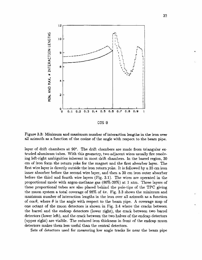
Figure 3.3: Minimum and maximum number of interaction lengths in the iron over all azimuth as a function of the cosine of the angle with respect to the beam pipe.

layer of drift chambers at 90". The drift chambers are made from triangular ex- truded aluminum tubes. With this geometry, two adjacent wires usually fire resolv- ing left-right ambiguities inherent in most drift chambers. In the barrel region, 30 cm of iron form the return yoke for the magnet and the first absorber layer. The first wire layer is directly outside the iron return yoke. It is followed by a 35 cm iron inner absorber before the second wire layer, and then a 30 cm iron outer absorber before the third and fourth wire layers (Fig. 3.1). The wires are operated in the proportional mode with argon-methane gas (80%-20%) at 1 atm. Three layers of these proportional tubes are also placed behind the pole-tips of the TPC giving the muon system a total coverage of 98% of 4n. Fig. 3.3 shows the minimum and maximum number of interaction lengths in the iron over all azimuth as a function of COS^, where 8 is the angle with respect to the beam pipe. A coverage map of one octant of the muon detectors is shown in Fig. 3.4 where the cracks between the barrel and the endcap detectors (lower right), the crack between two barrel detectors (lower left), and the crack between the two halves of the endcap detectors (upper right) are visible. The reduced iron thickness in front of the endcap muon detectors makes them less useful than the central detectors.

Sets of detectors used for measuring low angle tracks lie near the beam pipe

33

cos e

Figure 3.4: Coverage map of one octant of the muon detector system as a function of azimuth angle and cosine of the angle with respect to the beam pipe. The cracks between two barrel segments (lower left), the barrel and endcap segments (lower right), and the two halves of the endcap detectors (upper right) are visible.

34

on either side of the TPC [52]. Each of the two detector sets contains five drift chambers for tracking, an NaI low angle shower detector, a lead-scintillator large angle shower detector, a two plane scintillating hodoscope for time of flight, a muon detector, and a Cherenkov detector. The five drift chambers have position resolution around 300 pm, angular acceptance from 22 mrad to 180 mrad, and provide a momentum measurement with resolution ( U ~ / P ) ~ = (0.025)2 + (0 .008~)~ . The NaI detector contains 60 crystals each 22 inches long and hexagonal in cross-section (6 inches apex to apex) with an energy resolution of u*/E z 0.9% at 14.5 GeV (best performance without radiation damage). The lead-scintillator shower detector has angular acceptance from 100 mrad to 180 mrad, spatial resolution N 1 cm, and energy resolution U E / E = 0.15/0. The time of flight scintillating hodoscope has a resolution of 0.3 ns. The muon detector consists of 1 m of iron and three drift chamber modules and has a spatial resolution of 220 pm. The Cherenkov detector with angular coverage from 22 mrad to 180 mrad is a 1 atm C02 radiator 70 cm long. Its efficiency for electrons is greater than 90% overall and greater than 95% over 80% of its angular coverage. Typical trigger thresholds for the electron tagging system are E > 2 GeV in the NaI (double tag trigger) and E > 4 GeV in the NaI in coincidence with an extra charged or neutral particle (single tag trigger).

3.2 The Time Projection Chamber The primary detector used for this analysis was the Time Projection Chamber. In this section the device itself is first discussed, then the calibration and performance.

3.2.1 Description Of The TPC The Time Projection Chamber (TPC) is a gas filled cylindrical detector which provides 3-D images of tracks from charged particles and ionization energy loss ( d E / d x ) information [48]. The ionization along a track is drifted in an axial electric field to the end planes which are equipped with a large array of proportional wires and position pads. The wire signals provide d E / d x , and radial and axial position information, while the pads provide azimuthal and axial position information. The axial or “z” position is determined from the drift time of the electrons in the electric field. A solenoidal magnetic field bends the tracks so the particle momentum is determined from the position measurements which give the curvature. The simultaneous d E / d x and momentum measurements provide particle identification.

Fig. 3.2 shows the field configurations in the TPC. The axial magnetic field is produced by the solenoidal coil. The axial electric field is produced by the central membrane at a negative voltage and the field cage, a series of equipotential rings at the inner and outer radii of the TPC. Prior to 1984 the electric field strength was 75 kV/m resulting in an ionization drift speed of 5 cm/ps. In the 1984 changes the electric field was lowered to 50 kV/m giving an ionization drift speed of 3.3 c m / p . (Halfway through the data taking the field was raised to 55 kV/m.) Decreasing the drift velocity improved the z position resolution as discussed below.

35

The MWPC detector planes are divided into 6 sectors, each with 183 sense wires spaced at 0.4 cm and operated in the proportional mode. The amplitude of the signal on a sense wire provides ionization ( d E / d s ) information, and the timing of the pulse determines the depth of the track in the TPC. Thus the wires give r, z, and amplitude information. Fig. 3.5 shows the wire configuration of a sector. The drift region and amplification region are separated by a shielding grid. Between the sense wires are wires for field shaping. In 1984 a gating grid was installed. This grid serves to reduce the space charge in the TPC drift volume due to positive ions created in the amplification regions. Only after a (loose) pretrigger condition is fulfilled, the grid is switched into the transparent mode (Fig. 3.5) and drift electrons can reach the sense wires [53]. By the time positive ions produced in the amplification region drift back to the grid wires, the grid is usually closed and the ions are discharged at the grid wires. The gating grid greatly reduces electrostatic distortions, improving the momentum resolution. Azimuthal information is obtained from induced signals on 15 rows of rectangular cathode pads 0.75 cm high and 0.70 cm wide with spacing of 0.05 cm between pads. The cathode pads are 0.4 cm behind the sense wires (Fig. 3.5). There are 1152 pads per sector. Fig. 3.6 shows the relative position of the strips of cathode pads in a sector. This geometry provides 2 or more 3-d points and 15 or more wire signals per track over 97% of 47r.

The signals on the sense wires and pads are amplified and shaped before being sampled by charge coupled devices (CCD’s) which provide pulse height measurements at 100 ns intervals [54]. The CCD’s hold a 45.5 ps history (445 CCD buckets). On readout, the CCD clock frequency is changed from 10 MHz to 20 kHz allowing time for the signals in the CCD to be digitized. Each digitized signal is compared to a threshold for that channel stored in a RAM, and is read out to a buffer memory only if it is above the threshold. The shaper amplifiers were designed so an ionization pulse typically has 5 to 7 samples above threshold (see Fig. 4.1), thus providing enough information for good time (z) and pulse height resolution.

3.2.2 TPC Calibration And Corrections Both tracking and dE/ds determination in the TPC require very precise charge measurements. To achieve the required accuracy for the ionization and spatial position measurements, each channel must provide charge information which is both accurate and stable to better than 1% [55,56]. Several corrections must be applied to the raw pulse-height data from the TPC so it accurately reflects the ionization produced in the TPC volume. The size of a pad or wire signal depends on temperature, pressure, and composition of the TPC gas, the absorption of drift electrons by electronegative impurities, the gas gain as determined by the local geometry of the sense wire and cathodes, and on the transmission and recovery characteristics of the preamp, CCD, and digitizer. In addition, the measurement of the z-coordinate via the drift time requires precise knowledge of the drift velocity as well as propagation delays in the readout system. Calibration constants related to gas composition or detector temperature are usually time dependent.

The TPC electronics calibration is performed in two stages. First, the pedestal

36

(Drift Region)

Shielding Grid o 0 0 0 0 0 0 0 0 0 0 0 0 0 0 0 0

(Amplification Region)

- o x o x o x o x o Field Wires

Sense Wires 2 c--------) 4 mm

Cathode

Voltages

Midplane Gating Grid

Shielding Grid Field Wires Sense Wires Cathode

-55 kV -910 v f 90 v

* o v o v 700 V 3400 V o v

(Opaque Mode) (Transparent Mode)

8 mm

4 mm

4 mm

Figure 3.5: Wire configuration of a sector. The sense wires are operated in the proportional mode, and together with the induced signals on the segmented cathode, provide z, y, z, and amplitude information.

37

Cathode Pads

f Alternating \ LField and S e n s e 1

Wires

Figure 3.6: Relative position of the 15 strips of cathode pads.

levels are determined by setting the digitizer thresholds to zero and reading out the CCD’s. A least squares straight line fit to the measurements gives the pedestal slope (due to leakage currents, the pedestal increases over a full CCD readout by typically 1-2% of a pulse height for a minimum ionizing track) and the rms noise. The second step in the calibration is to measure the shape of the amplifier’s gain curve. The shielding grid (see Fig. 3.5) is pulsed at different voltages with a precision pulser and the gain of the wires and pads is measured and parameterized by an 11 point spline fit.

After a pulse is amplified, the amplifier output undershoots by about 0.5% of the pulse height, lowering the pedestal value for the remainder of the CCD read-in time. This biases any second ionization pulse to a lower value by about 0.5%. This effect is corrected, removing an observed dependence of the measured pulse heights on the number of tracks per sector.

Gas gain corrections are done in several steps. An initial calibration determines fixed correction factors (such as for variations in wire diameter) for each wire. Then time varying correction factors for continuously measured quantities (such as for TPC gas temperature variations) are applied on an event by event basis. Finally, run to run corrections are made which account for longitudinal diffusion and electron capture, and all remaining effects.

The calibration is done using a map of the wire gain made before the sectors were in place and then finding in situ corrections to the map. The map of the wire gain was made using an 55Fe line source to determine the relative gain every 4 degrees in azimuth along the wires. These relative gains were shown to be constant as long as the sector was not changed mechanically. The observed fluctuations were on the order of 3% rms and were due to variations in the diameter of the wire and variations in the distance from the wire to the cathode [55]. In addition, the heat

38

from the wire preamps, in spite of water cooling, caused a 3% increase in the gain in the vicinity of the preamps.

Since the environment of the sectors is different in the detector from that in the test system, the gain maps alone can not be used as a calibration of the gain at the sense wires. In situ calibration is necessary. Each TPC sector is equipped with three 55Fe line sources which can be moved pneumatically from behind screens to irradiate the wires. The 55Fe emits monoenergetic 5.89 keV X-rays which ionize K shell electrons in the argon. 85% of the time an Auger electron is emitted in addition to the primary electron and both travel a distance on the order of microns before loosing their energy by d E / d x . The ionization is collected on a single wire providing the main calibration peak N 5.89 keV. The other 15% of the time a photon is emitted, resulting in satellite peaks. Corrections to the initial gain maps from this calibration are of order 1-2% [57]. In addition, this data is used to eliminate sector to sector and wire to wire gain variations which are on the order of 15%. The reproducibility of the endplane source measurements has been extremely good with changes less than 0.3% over periods of six months [55]. The calibration is performed once or twice a month.

Quantities like gas pressure, temperature, and sector voltage which affect the proportional amplification are continuously measured and are read out with each event. Corrections for any changes are made to the data. A 1% change in the sector voltage causes an 18% change in the gain, a 1% change in gas density causes a 9% change in the gain, a 1% change in the CH4 fraction causes a 10% change in the gain, and a 1 “C change in temperature makes a 3% change in the gain [55]. Changes in the proportional amplification affect d E / d x measurements.

Longitudinal diffusion and electron capture by electronegative contaminants in the gas biases the ionization measurements to lower values for longer drift distances. The effect is typically between 5% and 13% over one meter [57]. This effect is monitored on a run by run basis (i.e. typically once per hour) and is corrected for.

After these corrections, a global d E / d x normalization factor is determined from the data for each run by looking at tracks with momentum between 400 and 600 MeV/c. In this region pions are minimum ionizing and are well separated from kaons and electrons (see Fig. 5.5). The mean d E / d x value for these tracks (the mean of the truncated means) is corrected to be 12.1 keV/cm (because early theoretical work predicted this value) and other dE/da: measurements are then made relative to this value. d E / d x measurements are discussed further in section 5.1.

In addition to the run to run corrections to the ionization measurements, there are also corrections that have to be made on a track by track basis. For example, when determining d E / d s , the amount of ionization per unit track length is required, so the effects of dip angle must be included. The track length sampled by each wire increases with dip angle. Also, the amount of ionization per unit track length depends on the logarithm of the length of the track sample. The dip angle correction includes this “log(1ength)” effect. After these corrections are made, the d E / d s of minimum ionizing pions is plotted as a function of time, azimuth, and dip angle. Any remaining dependence on these variables is removed with ad hoc corrections which are typically less than 3% [58].

39

A final quantity that must be accurately known is the drift velocity since it affects the z position resolution. It is found by monitoring the arrival time of ionization from cosmic ray tracks that cross the TPC midplane. Further refinements are made during data taking by monitoring Bhabha events and the endpoint of the arrival time distribution in multihadron events. The variation in drift velocity over the entire 1985/86 running cycle was around 7%, and the drift velocity was determined to 0.03%.

3.2.3 Position Measurement In The TPC The 15 pad rows on each sector provide x-y position measurements for up to 15 points along a track. Signals are induced on a given pad from the five wires nearest the pad, and an avalanche on a given wire can induce signals on either two or three pads. The x position (along a pad row) is found by fitting the response of the pads to a Gaussian. For 40% of the measurements, three pads are above threshold and the width of the Gaussian can be determined by the fit. If only two pads itre above threshold, the average measured width is used as input to the Gaussian fit.

The y position (perpendicular to the pad row) is calculated as the average position of the five wires that contribute to the pad signals, weighted by their pulse heights and coupling to the pad. This method reduces the effects of ionization fluctuations.

The z position of a spatial point is given by the average of the z positions determined by the pad signals. On any individual pad, an arriving pulse is shaped and sampled by the CCD. In the analysis, the samples are used to reconstruct the pulse and the position of the peak determines the arrival time. The z position is given by the product of the arrival time and the drift velocity.

After the 15, or so, spatial points on a track have been measured, corrections are made for known electrostatic distortions. Positive ion distortions affect the position measurement at small radii (the first pad row). In the older data set their magnitude was on the order of 1 cm, however, with the addition of the gated grid, they were negligible in the newer data set. Local electrostatic distortions caused by charge buildup on the field cages affect both the first and last pad rows. Their size is on the order of 1-2 mm for both the old and new data sets. Distortions from large scale electric field irregularities in the volume of the TPC are on the order of 1 mm for both the old and new data sets.

Since pulse heights are used to find position, factors determining the position resolution me the electronics calibration, electronic noise, diffusion in the 1 m drift distance, and ionization fluctuations [59]. A further factor is an E x B effect near the sense wires. This affects the resolution through a transverse force due to the fact that the electric and magnetic fields are no longer parallel.

The x-y position resolution is plotted in Fig. 3.7. For the newer data set, many things, including the electronics calibration, contributed a floor of 85 pm to the error on x-y position measurements. Electronic noise contributed 62 pm with an rms variation of 25 pm depending on the position and orientation of the track with respect to the pad row. The floor and noise contributions can be added in quadra-

- t +

40

220

200

180

160

140

n 120 E 2 100

80

6 0

40

20

0

c

-0.4 0 0.4

Tan( a)

Figure 3.7: Position resolution crzy as a function of the tangent of the azimuth angle a.

41

ture resulting in a fixed error of 105 pm. The x-y position error from transverse diffusion is proportional to L3, P-3, and ( l + ( u ~ ) ~ ) - T , where L is the drift distance, P is the pressure, o is the electron cyclotron frequency, and T is the mean electron collision time. For a one meter drift the error averaged over azimuth is 64 pm with an rms variation of 8 pm. Ionization fluctuations contribute an error which varies strongly with azimuth, as does the error due to E' x B' effects. To illustrate this, consider a track whose projection on the endplane makes an angle a with respect to the normal to the wires. If a # 0, an ionization fluctuation on one of the five wires contributing to the two or three pad signals will bias the pad response to larger values near the fluctuation. This will shift the measured x position. Weighting the five wires with their pulse heights to determine the y position partially compensates for this. The error is proportional to tan(a). In addition, for a # 0, the x-y resolution is affected by the E' x B' force near the wires which broadens the ionization pulse along the wire. Ionization fluctuations and the I? x $ effect contribute to the resolution about 200 pm times the angular dependence. All effects are combined in Fig. 3.7 which shows the x-y position resolution as a function of tan(a) over a sector (-30" < cy < 30"). The non-symmetric shape is due to the 2 x B' effect.

For comparison, in the older data set the fixed position error was about 160 pm, the error from transverse diffusion was about 105 pm (for a 1 m drift), and the error from ionization fluctuations was about 250 pm. The I? x 5 effect was not important with the lower magnetic field strength. The 1984 electronics calibration improvement is largely responsible for the smaller fixed position error in the newer data set. The increased magnetic field strength is responsible for limiting transverse diffusion, giving a smaller error from this contribution.

The position resolution in z is determined by the uncertainty in the arrival time of an ionization pulse, the drift velocity, and the t o calibration. The main factors that contribute to the uncertainty in the arrival time of an ionization pulse are the CCD sampling rate, ionization fluctuations, electronic noise, and longitudinal diffusion. Under present conditions, the CCD sampling rate gives the largest contribution. Since the CCD sampling rate did not change in 1984, the uncertainty in the arrival time of a pulse did not change significantly. However, the decrease in drift velocity improved the z position resolution proportionally, from 340 pm to 200 pm (averaged over dip angles).

The measured z position resolution as a function of dip angle is shown in Fig. 3.8. The z position resolution depends strongly on the dip angle (angle with respect to the midplane) of a track since the ionization pulse broadens with dip angle, making it more susceptible to electronic noise.

3.2.4 Momentum Measurement In The TPC The momentum of a charged particle in the TPC is determined by first fitting an orbit to the measured spatial points, taking into account the energy loss along the track. The inner and outer drift chambers are not used in the fit. A vertex fit then constrains the orbits to go through a common origin, consistent with the beam position. Only those tracks are included in the vertex fit, which do not raise the

42

n

E =L Y

360 1 Z Resolution 320

280

240

200

160

120

80

4 0

0 -0.8 -0.4 0 0.4 0.8

Tan (A)

Figure 3.8: Position resolution crz as a function of the tangent of the dip angle A.

43

600

4 0 0

200

0 -0.06 0 .o 0.06

Delta Curvature

Figure 3.9: Distribution of curvature difference for cosmic rays as measured in two different sectors.

global x 2 of the fit by more than 30. For tracks included in the vertex fit, the result of this constrained fit is used in the analysis. Note that since the TPC measures true space-points, three points or two points and the common vertex are sufficient to measure the momentum of a particle.

The error on the momentum has two contributions: position measurement errors and multiple scattering. The drastic reduction of beam related electrostatic distortions for the second data sample resulted in much smaller position measurement errors on both the inner and outer pad rows, essentially adding two points to the track fit. In addition, the improved position resolution reduced the component of the momentum uncertainty due to measurement errors. Increasing the magnetic field in the TPC from 3.89 kG to 13.25 kG improved both the measurement and multiple scattering components of the momentum resolution by the ratio of the field strengths. The measured momentum resolution was ( ~ , / p ) ~ = (0.06)2 + ( 0 . 0 3 5 ~ ) ~ prior to 1984, and at present is ( ~ , / p ) ~ = (0.015)2 + ( 0 . 0 0 7 ~ ) ~ ( p in GeV/c) for the fit with the vertex constraint. Without the vertex constraint, the measurement error contribution to the momentum resolution increased from 0 . 0 3 5 ~ to 0 . 0 6 ~ in the first data set, and from 0 . 0 0 7 ~ to 0 . 0 1 1 ~ (p in GeV/c) in the second data set.

The measurement error component of the momentum resolution was determined by comparing the curvature of cosmic rays as measured in two opposite sectors. A constraint that the two halves of the track meet at a common vertex was imposed. The distribution of the curvature difference is shown in Fig. 3.9 for the new data. A Gaussian fit gives

- OP = 0.007 (GeV/c)-'. P2

This value was checked with Bhabha and p+p- events where the momenta of both

.. .

44

1000

800

600

400

200

0 ii

1

- 0.08 0 0.08

Curvature (in units GeV- ’ )

Figure 3.10: Curvature distribution for tracks in p+p- events.

particles is 14.5 GeV (broadened by bremsstrahlung). Fig. 3.10 shows the curvature distribution for particles in p+p- events. The peaks for positive and negative particles are separated and symmetrical around zero curvature. The width of the peaks correspond to a momentum resolution consistent with the cosmic ray result.

The quoted multiple scattering contribution to the momentum resolution is calculated using the formula in Gluckstern [60].

3.3 Trigger

The trigger system for the TPC detector uses information from the drift chambers, the TPC, and the calorimetry, and is designed to provide high efficiency not only for annihilation events, but also for low-multiplicity two-photon reactions.

The trigger for the TPC [61] is composed of two parts, a pretrigger and a second level trigger based on a limited pattern analysis. The PEP beam crossing time is 2.44 ps and the ionization drift time from the midplane to the endcap of the TPC

45

is about 30 ps with 3.3 cm/ps drift velocity. The pretrigger uses TPC tracks which go through the endcaps providing prompt signals and the prompt signals from the inner and outer drift chambers. Beam crossings of possible interest are selected within 2 ps, leaving about 500 ns for clearing the analog systems if no pretrigger is generated. If a pretrigger is generated, the second level trigger uses the TPC wire signals to search for continuous tracks which come from the beam crossing position. This takes about 35 ps, limited by the ionization drift time. In the event of a second level trigger, the TPC is read out, requiring about 100 ms. The pretrigger rate is about 1 kHz corresponding to a trigger decision dead time of about 3%. The trigger rate is 1-2 Hz, resulting in an electronics dead time of 10%-20%. The TPC can trigger on 2 or more charged particles over 85% of 47r. The trigger efficiency for multihadronic events is larger than 99%. The calorimeters are used to supply a neutral energy trigger if there is 2 GeV or more of neutral energy in the hexagonal calorimeter or 1 GeV or more of neutral energy in the pole tip calorimeter (with two clusters required), or energy in two or more calorimeter modules each with more than 0.7 GeV. A charged+neutral trigger is formed if there is one or more charged tracks in the TPC and neutral energy of 750 MeV or more.

46

Chapter 4

Event Reconstruction, Selection, And Simulation

This chapter describes the method used to reduce the data samples of 77 pb-' taken in the 1982/83 running year and 67 pb-' taken in the 1985/86 running year to data summary tapes. A further event selection was used for this analysis and it is also described. Finally, because of its importance in the analysis, the Monte Carlo used for event simulation is discussed.

4.1 Event Reconstruction The events which trigger the TPC are reconstructed in an iterative procedure. After the application of calibration constants to determine pulse heights and drift distance, a pattern recognition algorithm finds approximate orbits. The resulting knowledge about the direction of a track crossing a pad row is used to determine second-order, orbit dependent corrections. These corrected points are used in the final fits.

The first step in analysing an event is to find the spatial points in the TPC volume from the corrected sense wire and pad signals. Fig. 4.1 shows the signals on three neighboring pads as a function of CCD sample number. The signal from each channel is first examined as a function of CCD sample number, and contiguous samples are combined to give an arrival time and pulse height by fitting the three largest samples to a parabola. The arrival time is corrected for the relative timing of the CCD clock with respect to the beam crossing. The z position where the ionization originated is then calculated using the measured drift velocity. The pulse height is corrected using the electronics calibration. Spatial points are then roughly found by searching for contiguous pads with signals roughly at the same z . The 5

position along the pad row is given by the average of the pad positions weighted by the pulse heights, and the y position perpendicular to the pad row is set to the centerline of the pad row. The z position is the weighted average of the z positions of the individual pad signals. Track finding algorithms connect the rough spatial points to form a first order set of tracks in the event. This is done online.

47

3

2

1

9

0 20 40 60 80 100 120 140 160 CCD Bucket Number

*

Figure 4.1: CCD samples above threshold from three pads.

48

The track finding program for high multiplicity events makes histograms in sin X (A is the dip angle with respect to the midplane) of the spatial points for each sector. For each bin in the histogram, the program chooses test points starting at the outer radius and moving inward. For each test point, it goes through the other points in the bin and makes a histogram of the sagitta of the circle that goes through the origin. Peaks in the histograms are taken as track candidates. The points in the peaks are then fit to a helix. Any points causing large residuals are excluded. In the end, a clean up procedure combines pieces of the same track together and adds points that had not been found before. The procedure is around 98% efficient at finding tracks which traverse many pad rows, and around 50% efficient at finding short tracks which traverse only three pad rows.

At this stage, time-dependent correction factors are determined from the data and updated. The beam-beam interaction point is measured as the average of the fitted event vertices. The drift velocity is measured by monitoring the endpoint of the ionization arrival time distribution. Gas gain at the sense wires is monitored using the dE/da: of minimum ionizing pions. Also, electrostatic distortions are monitored using the residuals of points in the track fits. Those corrections are averaged over an event sample (typically a 1 hour run) and are then applied in a second-pass, offline analysis.

In the next stage of the analysis, wire signals are associated with all tracks previously found using pads. A wire signal is associated with a track if its z position is within 0.7 cm of the original fitted track (1 cm in the older data set because of the increased drift velocity). However, a wire is excluded if the track to be associated with it is ambiguous, or if the pulse height is uncertain for some reason (if there is a neighboring large pulse which could cause crosstalk, or if there is another wire hit close in time which would affect the electronics). 65% of the tracks have 80 or more wire signals associated with them. The wire signals are used to determine the particle’s d E / d x , as discussed in chapter 5.

The wire pulse heights and track information are used to refine the pad space points. The a: position along the pad row is determined by a Gaussian fit to the pad signals, and the wire signals are used to find the y position, perpendicular to the pad row. Tracks are then refit to the refined space points. These refined tracks are used in the final fit which constrains all tracks to come from the event vertex.

Fig. 4.2 shows a typical multihadron event in the TPC from the 1985/86 data set. The reconstructed tracks have been labeled. In the side view all points have been rotated about the beam axis to lie in a plane.

4.2 Multihadron Event Selection After the event reconstruction, a selection is made to separate multihadron events which are then put on data summary tapes (DST’s). The multihadron DST’s are the source of data for this analysis. The criteria for an event to be put on the multihadron DST’s are discussed below.

The tracks used to select multihadron events are “good tracks” which pass the

49

EXP= 1 4 , RUN= 7, EVENT= 872, P I X I D = 1 T R G = ' 1540'0 PNL= '20000200 'X ANL=' 20000'X

1

4

Figure 4.2: Typical multihadron event in the TPC from the 1985/86 data set.

50

following cuts. (1) The angle of the track with respect to the beam pipe must be larger than 30” to ensure that the track is in the fiducial volume of the TPC. (2) The error on the measured curvature of the track must be less than 0.3 GeV-’ or the curvature error has to be less than 30% of the curvature. This is to ensure a good momentum determination. (3) The measured momentum of the particle must be larger than 0.12 GeV to remove particles coming from nuclear interactions in the material in front of the TPC. (4) The extrapolated origin of the track must be within 6 cm in the x-y direction, and 10 cm in the z direction (along the beamline) of the nominal vertex. This is to eliminate tracks not associated with the event such as those from cosmic rays.

The “good tracks” defined above are used to select multihadron events. To be considered a multihadron event, an event must meet the following criteria. (1) The event must have at least five good tracks in the TPC which are determined to be non-electrons either by dE/da: or by a pair finder program which geometrically re- constructs conversion pairs. The restriction to non-electrons is to eliminate Bhabha events where the electron or positron showered in the material in front of the TPC. (2) The observed energy of charged particles, E&, has to exceed 7.25 GeV. This cut is used to eliminate 2-photon events. (3) The net momentum along the beam pipe of the charged particles must be less than 40% of E c h / C . This cut eliminates events with large initial state radiation and also reduces contamination from two- photon events. (4) The majority of the tracks in the event have to be good tracks in the sense defined above. ( 5 ) To reject T events two hemispheres along the jet axis are constructed. In at least one hemisphere the event must have more than three charged tracks, or the invariant mass of the charged particles in the hemisphere must be larger than 2 GeV. (6) The reconstructed vertex of the event must be within 2.0 cm in x-y and 3.5 cm in z of the nominal vertex.

With these standard multihadron event selection criteria, contamination is estimated to be 0.3 f 0.1% from TT events, 0.8 f 0.6% from two-photon events, and less than 0.1% from beam gas events and Bhabha scattering.

For this analysis, not all the “good tracks” on the multihadron DST’s were used. Only those that met the following additional criteria were accepted. (1) The error on the measured curvature of the track had to be less than 0.15 GeV-’ or the curvature error had to be less than 15% of the curvature. (2) The measured momentum of the particle had to be larger than 0.15 GeV. (3) The extrapolated origin of the track had to be within 3 cm in the x-y direction, and 5 cm in the z direction of the nominal vertex.

To be considered for this analysis, an event on the DST still had to have 5 or more good tracks as defined in the preceding paragraph. In addition, it was required that the polar angle of the event axis with respect to the beam pipe had to be larger than 45”. This was done to ensure that a large majority of the particles in each event were in the fiducial volume. For the older data set 21434 events survived these cuts, and 20270 events survived in the newer data set.

51

c

4.3 Event Simulation Monte Carlo event simulation is essential in understanding detector performance. The TPC group uses two Monte Carlo detector simulations, a full simulation which generates raw data for all detectors, and a simulation designed for speed, the Fast Monte Carlo, which generates space points and fits them producing DST output. For determining the acceptances and particle misidentification probabilities needed for this analysis, the Fast Monte Carlo was used because high statistics were needed.

The Fast Monte Carlo [57] uses a physics generator (Lund, Webber, . . . ) to produce input events. Initial state radiation is simulated using the program of Behrends and Kleiss [62]. The event vertex is chosen in accordance with the PEP beam size. Both charged and neutral particles are tracked through the detector and long lived particles are allowed to decay in the detector volume. Pad hits are generated for charged particles in the TPC and a fit to the points gives the particle’s momentum. A d E / d x value is calculated. The output is written in the standard DST format with an additional block containing information about the generated event.

The Fast Monte Carlo models the TPC as a series of discrete layers, each of uniform density. The beam pipe, pressure wall, inner drift chamber, and field cage each constitute a single layer, as does the full distance between pad rows in the TPC. Charged and neutral particles are tracked from layer to layer. The effects of energy loss, multiple scattering, bremsstrahlung, decay in flight, and nuclear interactions are included for charged particles. Neutral hadrons can interact in material and photons can convert to e+e- pairs. Pad hits are generated for charged particles at the appropriate layers by smearing the tracked position with a resolution function that includes the effects of diffusion, dip angle, electrostatic distortions, and the electronics. Inefficiencies due to missing electronic channels, sector boundaries, and track overlap are included.

Individual wire hits are not generated. Rather, a particle’s d E / d x is calculated using its average ,By in the TPC, and then smeared. The d E / d x resolution used for the smearing is the measured resolution depending on the number of wires and the dip angle (section 5.1). In determining the number wires, effects of sector boundaries, track overlap, and missing electronics channels are included, in addition to the TPC geometry.

Pattern recognition in the Fast Monte Carlo is done using a simple algorithm for speed. Measured pad space points within 3 cm of a track are associated with that track, and any track with 3 or more space points is assumed to be found. Ambiguous space points are assigned to only one track. A vertex constrained fit giving the particle momenta is performed in a manner equivalent to the real data analysis.

In the region within the cuts used for this analysis, the Fast Monte Carlo agrees with the experimental data very well, as illustrated in Fig. 4.3.

cn U C Q) >

W CL 0 L Q n

Z 5

v) Y C a, >

W

2

5 L Q) n

z

cn Y 0 I) L I- CL 0 L a, n

Z 5

60004

4000-

0 5 10 15 20 25 Number OF Hadrons

L

(dl 1500

1000

500

100000!.

80000

60000

U

-0.4 -0.2 0 0.2 0.4 CP I / XES-

(e)

I I . . I

0 0.05 0.1 0.15 0.2 AC WGeW

(F) L 14

cn U C Q >

W

0

n

z

L

L Q

5

v) 3 0 II L c 8

5 L a, n

z

v) Y 0 I) L c (r, 0 L Q) 9

Z 5

600

500

400

300

200

100

'0 5 10 15 20 25 30 CEchwqd trwk

Number OF dE/dX Samples

Figure 4.3: Comparison between the data (points) and the Fast Monte Carlo (histogram). (a) The number of charged hadrons. (b) The sum of the energies of good tracks. (c) The momentum balance (E p, / E) along the beam direction. (d) The number of d E / d x samples along a track. Negative numbers indicate pads were used in the d E / d x calculation rather than wires due to track overlap. (e) The curvature error AC for tracks with p > 1 GeV. ( f ) The relative curvature error AC/C for tracks with p < 1 GeV.

53

Chapter 5

Particle Identification By d ~ / d z

5.1 Theory And Measurement Of Ionization En= ergy Loss In The TPC

Effective particle identification by dE/dz requires the precise knowledge of the expected ionization energy loss as a function of particle mass and momentum. For the TPC analysis, the velocity dependence of the energy loss is taken from a rather detailed theoretical calculation, to which small empirical corrections are applied for best agreement with the data. The calculations were heavily based on the work of Lynch [63], Lapique and Piuz [64], Allison and Cobb [65], and Talman [66].

The cross section da/dE for an incident particle to loose energy E in a collision with an atom of a gas is approximated by [65]

da do d o dE dE dE Rutherford - = (-)resonance + (-)

where

da E dE'. ( E ) R u t h e r f o r d = -- P2r cy E 2 ' I T

ay(E) is the photoabsorption cross section for a photon of energy E , ,9 is the incident particle's velocity, Z is the atomic number of the atom, m is the electron mass, cy is the fine structure constant, and €1 and €2 are the real and imaginary parts, respectively, of the dielectric constant of the gas which can be expressed as a function of the photoabsorption cross section. For notational convenience, the gas is assumed monatomic, but the extension to mixtures is straightforward. A term representing Cherenkov radiation has been ignored since it is small in the TPC. The first term labeled ret~onance depends on o,(E) and is large at the ionization thresholds. The main feature of this term, however, is the strong ,8 dependence which allows relativistic particle identification. The Rutherford term represents the contribution from hard scattering off electrons. In the regions of E near the photoabsorption peaks, the Rutherford contribution to the cross section is smaller than

54

the resonance contribution. However, at large E where a,(E) is small, the Ruther- ford term is the larger since it depends on J:ay(E')dE'. This gives a 1/E2 tail to the cross section. The expression for da/dE shows that the Rutherford scattering term with 1 / p 2 velocity dependence will be of little use in distinguishing relativistic particles with p N 1. Thus, to determine velocity, resonant energy loss must dominate dE/dx, not hard Rutherford collisions. This is achieved in practice by sampling the energy loss in thin layers of the gas, so that in any layer the probability of a Rutherford scattering is small.

The average number of interactions resulting in energy loss E in dE per unit path length dx is given by

da dxdE dE

= n- dN

where n is the number density of atoms in the gas. This expression yields the average number of interactions per unit length

dN da - = In-dE. dx dE

The actual number of interactions per unit path length d N / d x is distributed according to a Poisson distribution with mean value dN/dx .

A Monte Carlo program was written [57] to calculate the distribution of observed energy loss per unit path length for an incident particle with fixed velocity. For argon and methane separately, the photoabsorption cross section a,(E) was expressed in terms of the oscillator strength f ( E ) by

and the oscillator strength was approximated by a sum over atomic levels

where w; is the probability that an electron is found in atomic level i. The form of f ; ( E ) was taken to be

F(f-)-'i, for E > E; f ; (E> = { 0, otherwise,

where s; and E; are constants for level i. The atomic levels and values of s; and E; used in the Monte Carlo are given in Table 5.1. Using this expression for f ( E ) , dN;/dx was approximated for each atomic level and a value of dN;/dx was chosen according to a Poisson distribution. An average energy transfer per interaction was taken to be E i j j (Table 5.1) in the resonance region, and in the Rutherford region was chosen according to a 1/E2 distribution. The total energy deposited in dx was then calculated by summing the energy deposited in resonance and Rutherford collisions for each level i for the argon and the methane. The resulting distribution is shown in Fig. 5.1 along with the measured distribution. Its most striking features

55

Table 5.1: Table o

t

Atom Ar Ar Ar Ar

CH4 CH4

0.444 0.133 0.311

- 0.8 0.2

3206. 2.75 248. 2.29

15.8 3.20 11.5 2.15 283. 2.52

5341.

27. 506.

energy levels and relevant data used in the dE, -2 calculations.

1000

800

600

400

200

0 ' 0 6 10 15 20 25 30 35 40

dE/dx (keV/cm)

Figure 5.1: Distribution of energy losses in 4 mm of the 8.5 atm. argon-methane (80% - 20%) TPC gas.

56

are its broad shape and long tail (Landau tail [67]). Because the distribution is so wide, mgny measurements are needed to measure its shape or to form an estimator. Fig. 5.1 shows the intrinsic width (excluding the tail) of the energy loss distribution is N 60% of the most probable d E / d x value.

To associate the incident particle's velocity with the measured dE/dx distribution, it is desirable for practical reasons to have a single number, an estimator, reflect the distribution. The most probable dE/dx is not a good estimator for limited statistics [65], and the same is true of the mean. The quantity used to overcome this problem is the mean of a fixed fraction r of the measurements with lowest energy loss (i.e. the truncated mean). The resolution of the truncated mean was found to be insensitive to values of r in the range 0.4 5 T 5 0.7 [68]. We chose r = 0.65. The truncated mean will be referred to as the dE/dx value when talking about the estimator.

The measurement of d E / d x in the TPC proceeds along lines previously discussed. Ionization arriving at a wire undergoes proportional amplification. The wire signal is then amplified, shaped, and sampled 5 to 7 times by a CCD. Upon analysis, the three largest CCD samples are fit to a parabola to determine the pulse height, which is then corrected as previously discussed. Up to 183 wire signals can be obtained along a track. These individual measurements are then used to calculate a truncated mean.

In some cases the amplitude of the pad signals provides a more accurate d E / d s determination than the wire signals. In cases of track overlap, few wires are associated with a track. Since the pad signals integrate over several wires, the statistical significance of a pad signal is greater than for a wire signal. The pad signals are used to determine the dE/dx value if Npads 2 0.4Nwjres. This happens 12.9% of the time.

An assumption, which is widely accepted, is that the ionization I produced by a moving charged particle is proportional to its energy loss E , I = E / W , where the proportionality constant 1/W is independent of E [65]. We have assumed this, often speaking of energy loss and ionization equivalently.

The expected velocity dependence of the truncated mean was calculated using the formalism discussed above [58]. It was assumed the truncated mean d E / d x has the same velocity dependence as the most probable value, which is fairly easy to calculate.

The calculation proceeds along the same lines used to derive the dE/dx distribution, except a closed form expression is obtained. Again, the calculation is illustrated for a monatomic gas for simplicity, but the extension to mixtures is straightforward. The most probable energy loss AEmP in a thickness Ax of gas is approximated by the sum of a resonance and a hard scattering contribution,

A E ~ ~ o n , n , e is given by the sum over energy levels of the most probable number of interactions from level i, times the average energy loss per interaction. The most probable number of interactions from level i is the mean ( A x d N j / d z ) minus 1/2, since the number of interactions follows a Poisson distribution. The values of the

57

average energy loss E: for level i were obtained from the oscillator strength using the expression

00

In E: = 1 ln(e)fi(e)dc.

The f ; ( E ) used in the calculation are those given previously. Combining terms,

The expression used for the most probable energy loss due to Rutherford scattering was that of Maccabee and Papworth [69]

where 2ae4 1 & = -n;Ax-. me2 P2

From these expressions, and taking into account the gas mixture of the TPC, the most probable energy loss as a function of Pr = P / d V shown in Fig. 5.2 was obtained.

This theoretical curve was then used m the basic functional form in a fit to experimental data. The average truncated mean dE/dx as a function of Pr was measured for low energy protons and pions from multihadron events, cosmic ray muons, conversion electrons, and wide angle Bhabha electrons since all of these particles are easily identifiable. The P-y value was extracted from the momentum. The fit was of the form

ln(PY)trunc. mean = A Wy)predicted +

(dE/dx)trunc. mean = C(dE/dx)predicted + and is depicted in Fig. 5.3. The values of A, B, C, and D giving the minimum x2 were

A = 0.986

B = -0.055

c = 0.999

D = 1.532.

The resulting x2 per degree of freedom was 1.50, indicating a very good parame- terization of the truncated mean dE/dx as a function of Pr. A plot of the average R =(trunc. mean/prediction) as a function of /?r for pions and cosmic ray muons is shown in Fig. 5.4. It indicates the fitted dE/dx vs. /?r curve is accurate to 0.2%.

The fitted dE/dx vs. Py curve can be easily converted to a dE/dx vs. momentum curve for a given particle type by scaling the abscissa with the particle mass. When this is done, the solid curves of Fig. 5.5 are generated. The figure also shows our

58

I : I :

I *.

I 1 I I \

..****...........................* ...

I *e.

....

5 \ \

X -0

UJ U

............. R8SOMnW i 20 - - - - - Rutherford

Total

Figure 5.2: Calculated most probable energy loss per unit path length as a function of q = pf.

59

X Q

Q '2;

E

o--- i protons

conversion electrons

\ pions \ Y

cosmic Bhabha ray muons electrons

Figure 5.3: Fitted truncated mean dE/da: as a function of ,By showing the various experimental measurements used in making the fit.

60

1.02

o cosmic ray muons 1.01

R 1.00

0.99

0.98 50 10 50 100

PY

Figure 5.4: Plot of average R =(trunc. mean/prediction) as a function of Pr indicating the fitted dE/ds vs. Pr curve is accurate to 0.2%.

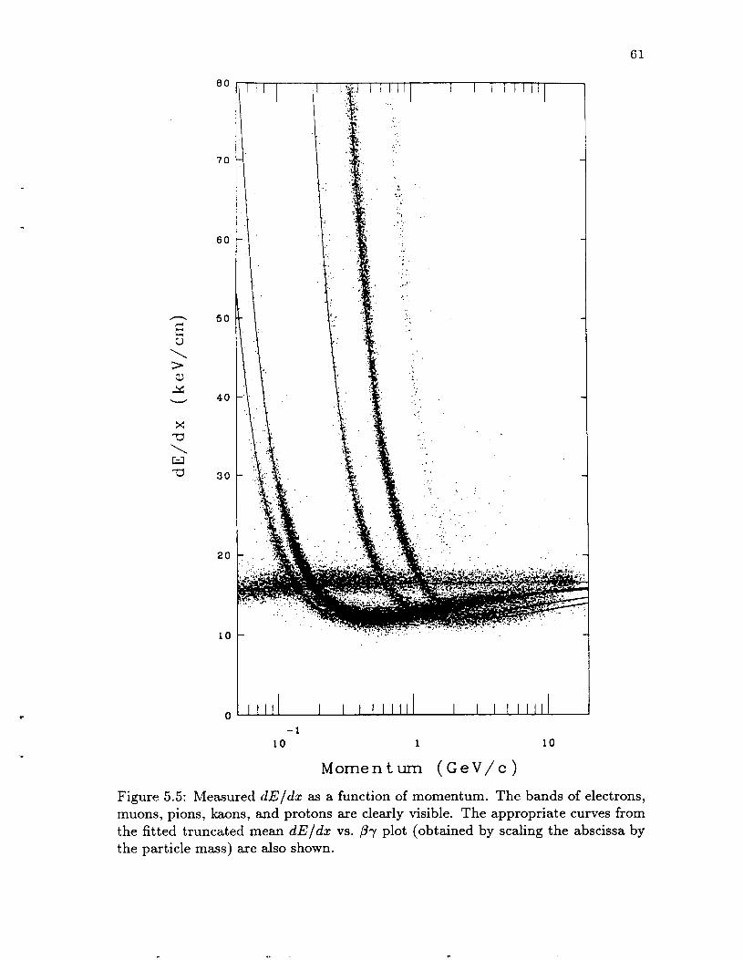
61

n

0 \ > c) x

E

W

X 3 \ w -u

80

70

60

5 0

40

30

20

10

0

Figure 5.5: Measured d E / d x as a function of momentum. The bands of electrons, muons, pions, kaons, and protons are clearly visible. The appropriate curves from the fitted truncated mean d E / d x vs. Py plot (obtained by scaling the abscissa by the particle mass) are also shown.

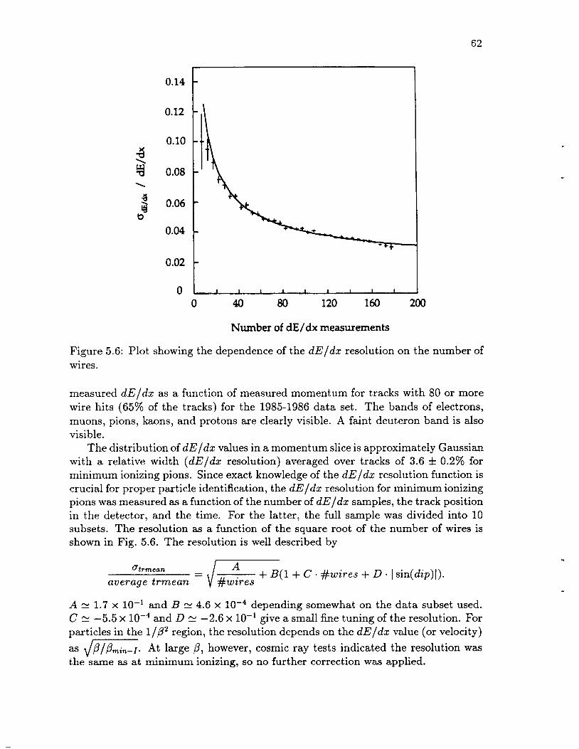
62

0.14 1 0.12

0.10

0.08

0.06

0.04

Figure 5.6: Plot showing the dependence of the d E / d x resolution on the number of wires.

measured dE/da: as a function of measured momentum for tracks with 80 or more wire hits (65% of the tracks) for the 1985-1986 data set. The bands of electrons, muons, pions, kaons, and protons are clearly visible. A faint deuteron band is also visible.

The distribution of dE/da: values in a momentum slice is approximately Gaussian with a relative width ( d E / d z resolution) averaged over tracks of 3.6 f 0.2% for minimum ionizing pions. Since exact knowledge of the d E / d x resolution function is crucial for proper particle identification, the dE/da: resolution for minimum ionizing pions was measured as a function of the number of dE/da: samples, the track position in the detector, and the time. For the latter, the full sample was divided into 10 subsets. The resolution as a function of the square root of the number of wires is shown in Fig. 5.6. The resolution is well described by

+ B( 1 + C #wires + D I sin(dip)l). ottmean

average trmean #wires

A N 1.7 x lo-' and B 21 4.6 x depending somewhat on the data subset used. C 11 -5.5 x and D N -2.6 x lo-' give a small fine tuning of the resolution. For particles in the 1/p2 region, the resolution depends on the d E / d x value (or velocity) as ,/=. At large ,B, however, cosmic ray tests indicated the resolution was the same as at minimum ionizing, so no further correction was applied.

63

3 10

lo2

10

1

Figure 5.7: Plot showing the distribution in S (as defined in the text) for minimum ionizing pions. The distribution is consistent with Gaussian of width 1 out to 3 S.D.

For minimum ionizing pions, the distribution in

trunc. mean - prediction predicted resolution

S =

is shown in Fig. 5.7 for tracks with at least 80 wires. The distribution is consistent with Gaussian of width 1 out to 3 S.D.

For tracks that use pads to determine the d E / d x , the resolution is considerably worse than for tracks that use wires. The resolution for tracks with at least 13 pads is 7.6%.

Overall, the average d E / d x resolution improved in 1984 because of better corrections. For Bhabhas it improved from 3.5% to 2.9%, and for tracks with 120 or more wire hits in jet events the d E / d x resolution improved from 4.0% to 3.4%.

Except in regions where the d E / d x curves cross, the energy loss measurement provides a separation between species of many S.D. at low momentum, and of 2- 3 S.D. in the high momentum region. A plot of relative d E / d x separation vs. momentum is shown in Fig. 5.8 (assuming a nominal resolution of 4%), from which the regions of good particle identification are evident.

64

I2

10

8

6

4

2

0 0.06 0.1 1 10 20

Momentum (GeV’c)

Figure 5.8: Plot showing the dE/da: separation in terms of the resolution as a function of momentum.

65

u) Y 0

I- #

E

0 . 7 0 . 8 0 . 0 I 1 . 1 1 . 2 1 . 3

(d E/dx)/( dE/dx),

Figure 5.9: At high momentum a sum of Gaussians can be fit to the dE/dx spectrum to determine the number of particles of each species present.

5.2 Particle Identification Algorithms In the 1/p2 region of the dE/dx vs. momentum plot, particle identification is easy since the dE/dx bands are widely separated (see Fig. 5.5). The measured momentum and dE/dx value uniquely determine the particle type. Cross sections and particle fractions as a function of momentum are easily found in this region by counting particles.

When the dE/dx bands overlap, one dimensional fits to the dE/dx spectrum determine the number of particles of each species in fixed momentum intervals. The dE/dz spectrum is expressed as a sum of Gaussians, one for each particle species. The area under each Gaussian gives the number of particles, from which cross sections and particle fractions are easily determined. This is illustrated in Fig. 5.9 for particles with momenta between 4.4 and 5.1 GeV/c. Such fits use the maximum amount of the information available, but the method is straightforward only for momentum distributions; it fails if particles are selected according to some other criteria such as rapidity or transverse momentum since the dE/dx spectrum

66

in a rapidity or pt interval is no longer a sum of Gaussians. When cross sections in rapidity or momentum transverse to an event axis are

desired, an unfolding technique provides an attractive alternative to one dimensional fits. For the distributions presented in this thesis, the same unfolding was used. Basically, some algorithm is used to identify particles; the raw rates are then corrected for misidentification using a “confusion matrix” derived from a Monte Carlo simulation. The procedure is discussed in detail in the following chapter.

67

Chapter 6

Measurement Of Inclusive Cross Sections

6.1 Definition Of Variables And Choice Of Event Axis

The cross sections presented in this thesis are

for pions, kaons, and protons (both + and - charges are combined). For each cross section the associated particle fractions are also given. E is the particle energy, p is its momentum, pll and pt are the components of momentum along and transverse to the event axis, respectively, and 4 = 29 GeV at the PEP ring.

The distributions involving rapidity (y) and transverse momentum ( p t ) require the definition of an event axis. The two most common choices are the sphericity axis and the thrust axis, and w e present distributions for both. The sphericity axis is determined by finding the direction of the unit vector n' that minimizes

3 p: sin' ei 2 C P ?

S(Z) = - 7

where the sums run over all charged particles. p ; is the magnitude of the momentum of particle i, and & is the angle between the direction of particle i and the vector n' that is being varied. The thrust axis is determined by finding the direction that maximizes

68

This expression is linear in the particle momenta, and therefore is more stable under fluctuations in fragmentation than sphericity.

As pointed out in [70], rapidity and pt distributions measured with respect to an event axis determined from the tracks themselves is, strictly speaking, not a truly inclusive measurement. Almost by definition, the choice of a jet axis will introduce some bias. Sphericity and thrust behave rather complementary in this regard, and their effect on inclusive distributions can be understood qualitatively as follows [71]. Consider the hypothetical case in which all tracks in an event lie in a plane. Suppose the direction of n' is close to extremizing S(Z) or T(n'), and consider the sensitivity of S(n') and T(n') to changes dB in the direction of n':

d S 2pf sin Bi COS 8,dB i

and d T - c( *)pi sin Bide,

i

where ( z t ) in d T accounts for the effect of the absolute value in 2'. From these relations several facts emerge regarding the final extrema of S and T :

1. Because of p: , the sphericity axis tends to align along fast tracks.

2. Sphericity tolerates low momentum tracks perpendicular to the axis.

3. Thrust avoids having particles perpendicular to the jet axis, even at the ex- pense of a minor misalignment of fast particles.

The influence of detector acceptance and momentum measurement errors on the direction of the sphericity and thrust axes was studied using a Monte Carlo [71]. The reconstructed axis using charged particles was compared to the "true" sphericity or thrust axis derived using all generated (charged + neutral) particles, the angle between them being 4 (always positive). It was found that the accuracies of the sphericity and thrust axes were identical and gave (4) N 9". However, if very poorly measured tracks were included, thrust was more reliable than sphericity as might be expected since it depends only linearly on the momentum. But for tracks measured with the typical TPC resolution, those used for this analysis, both methods were well within their range of stable operation.

Our Monte Carlo studies determined that the errors on the measured values of y and pt were due largely to errors in the determination of the jet axis. For the older data set, the resolution for measuring rapidity was uy 0.3 for y near zero and cy N 0.5 for large y. Of this, the contribution from momentum measurement error was uy fi! 0.1 for y near zero and uy N 0.2 at large y. Both sphericity and thrust gave similar results.

It was also determined in our Monte Carlo studies that the dip in du/dy at y = 0 is more pronounced using the thrust axis than the sphericity axis. This is borne out by the data presented here. The dip is easily understood from the previous discussion since thrust tends to remove particles perpendicular to the event axis (Y = 0).

.

69

X TI \ W U

Figure 6.1: The x2 assigned to an identity hypothesis is the “distance” in terms of the resolutions from the point (q,(dE/dx),,,eaa), q = pmeas/m,,ypot,,, to the d E / d x vs. q curve.

6.2 Unfolding Technique To Measure Cross Sec- t ions

The cross sections and particle fractions were determined in two steps. An algorithm was used to identify tracks in the TPC as electrons, pions, kaons, or protons. Then corrections derived from our fast detector simulation Monte Carlo were applied accounting for particle misidentification and detector acceptance. The process is described in detail below.

6.2.1 Particle Identification To identify particles, having measured the momentum and d E / d x in the TPC, different particle hypotheses (e,n,k,p) are tried and a x2 is determined for each hypothesis. The method for determining the x2 is illustrated in Fig. 6.1. The measured momentum divided by the hypothesized mass determines the abscissa

70

and the measured d E / d x determines the ordinate of a point in the plot. The x2 for the mass hypothesis is given by the distance of the point from the fitted d E / d x vs. Pr curve in terms of the d E / d x and momentum resolutions. The x: ( i = e, T, k,p) are converted to probabilities P; by incorporating guesses for particle fractions f ; ( p ) based on previous measurements. Our results are very insensitive to the values of f ; ( p ) used, since their effect on particle misidentification is corrected for, as discussed later. P; is defined as

P; = Nf;(p>e- M. N normalizes the sum of the P;. A particle is “identifiable” and considered of type j if the following criteria are met:

1. The number of d E / d x samples has to be larger than or equal to 40, and the d E / d x must not have been determined from the pad signals.

2. The ionization measured must not have saturated the electronics.

3. The x2 for hypothesis j has to be less than or equal to 10.

4. The probability of hypothesis j, P’, must be larger than or equal to 0.7.

Fig. 6.2 shows the distribution of the number of wires per track for tracks used in this analysis. 12.9% of the tracks use pads for d E / d x and 3.8% of the tracks that use wires have fewer than 40 wires, so 16.7% of the tracks are excluded by cut 1. This cut and cut 2 are needed to get an accurate d E / d x measurement. Cut 4 selects for the analysis only tracks with a high probability of being from a certain particle type. In the Monte Carlo, pions are identified correctly more than 95% of the time over the momentum range, while outside of crossover regions, kaons and protons are identified correctly more than 85% and 60% of the time, respectively, over the momentum range.

No attempt has been made to separate muons from pions. Since most muons come from pion decay, such a separation would rely heavily on the event generator Monte Carlo. Thus, our “pion” cross sections are actually pion+muon cross sections, including pions and a small number of muons from sources other than pion decay.

6.2.2 Unfolding The particles identified via the method just described are counted for each bin of the independent variable. This gives experimentally determined average numbers per event of electrons, pions, kaons, and protons M; ( i = e,T,k,p) for each bin. The M; are corrected for particle misidentification, detector acceptance, and initial state radiation by the matrix inversion technique we now describe.

There is some ambiguity regarding particle decays in defining the corrections. We correct to a “vertex” where particles with lifetimes shorter than lo-’ sec have decayed, leaving only the long lived particles y, v , e*, p*, 7r*, k*, kL, p, p, n, and n.

Let V, (i = e, 7r, k,p) be the actual average number of particles per event of type i produced at the e+e- interaction “vertex” with no initial state radiation and after

-

.

71

t

Wires Or Pads

Figure 6.2: Distribution of the number of wires per track for tracks used in this analysis. A negative number of wires indicates pads were used for dE/dx .

72

short lived particles have decayed. Particles and antiparticles have been lumped together, and T stands for pions+muons as discussed earlier. The V, are the desired quantities.

We define Ii (i = e, T , k,p) as the average number per event of particles of type i in the TPC which are “identifiable”, meaning the cuts of the previous subsection were passed. The I* and the V, are related by an expression I; = DijV,, or in matrix form

I = DV.

Dij is the probability that a particle of type j at the vertex produces an identifiable particle of type i in the TPC. Note that D is diagonal to a good approximation, and that Dii is essentially the probability that a particle of type i at the vertex makes it into the TPC and passes the cuts to be identified as something. (Small corrections and nondiagonal elements arise e.g. from nuclear interactions whose secondaries reach the TPC.)

Since the particle identification is imperfect, a particle of type j is labeled as type i with probability Cij. The average measured number per event M; of particles called i is Mi = CijIj, or in matrix form,

M = C I .

Note that the columns of C sum to 1. Combining equations gives

M = CDV,

and multiplying by the inverses of the matrices gives the desired result

V = D-’C-’M.

The C matrix describing particle misidentification depends on well-measured detector properties such as the separation in dE/da: between species and the dE/ds and momentum resolutions, and on the algorithm used for identification. Any dependence on the physics generator is very indirect (the angular width of jets, etc. influences track overlap in the TPC, and hence the average number of wire samples and the dE/dz resolution); in particular, the C matrix is independent of the particle composition created by the event generator. Changing the fractions f;(p) changes the Mi’s, and the C;j’s and Dij’s, but not the resulting X’s. This was in fact tested by using several sets of f;(p), among those a set of constant fractions fe = 0.05, fT = 0.75, fk = 0.15, and fp = 0.05 for all momenta. The resulting z distributions were computed and agreed with the distributions presented here within errors.

The D matrix is diagonal to a good approximation. Small nondiagonal elements are due e.g. to nuclear interactions in the beam pipe with a secondary in the TPC. Also, such effects as momentum smearing and initial state radiation, move tracks into different kinematical bins. Since all these corrections are small, instead of unfolding the data, we define an effective diagonal D matrix for a given bin as

73

follows:

# of particles of type i identified as something in the TPC

per generated event including initial state radiation # of generated particles of type i after decays

per event with no initial state radiation

D.. - t t - 7

,

D;j = 0 for i # j . D;i is the average number of particles of type i in the TPC in the given bin identified as something, divided by the average number of particles of type i in the given bin at a generator vertex with no initial state radiation. Thus the D matrix does the acceptance correction, the initial state radiation correction, and corrects for mismeasurement of the independent variable. A reliance on the physics generator is introduced since the particle fractions must be right to account for non-diagonal effects such as kaon decay before the TPC, although such effects are small. (If pions were separated from muons, the corresponding off diagonal term would be required since it would be large.) One possible large non-diagonal effect is pions, for instance, knocking protons from the beam pipe into the TPC. Only negative particles from the TPC were used in the analysis to avoid this problem, since the cross sections for such processes are not perfectly simulated.

When the generator is run without initial state radiation for determining D;i, the rapidity and pt bins a particle goes in are determined from the event axis calculated using only charged stable particles. So no correction is made to find the distributions using all particles (or some other scheme) to determine the event axis.

Figure 6.3 shows plots of the C and D matrix elements as a function of z = 2p/&. The d E / d x crossover regions are clearly visible in the plots of Cij as dips in Cii and peaks in Cij, i # j . The close p-n and p-k crossover regions leave nothing called a proton from z cx 0.12 to z N 0.22 making the C matrix singular in this region. Otherwise, the particle identification is very good. Since only negative particles from the TPC are used in the analysis, the maximum value of Di; in principle is 0.5. The electrons knocked out of the material in front of the TPC, however, make Del,e[ > 0.5 at low z. The effects of the crossover regions are visible in Dii since it includes a correction for the requirement that the particle be identified as something. Plots of the C and D matrix elements as a function of other variables are given in Figures 6.4 to 6.7. In these plots the pion mass was used compute the energy and rapidity, and the sphericity axis was used as the event axis.

A very important problem in the unfolding process is that the bin a particle goes in must not depend on the identity assigned to that particle, otherwise misidentification could move particles between bins. The bin a particle goes in should only depend on its measured momentum, even for variables like x which depend on mass. To see how this was done, consider the variable x = 2E/& which depends on the particle’s identification through the mass in the energy. First, the T , k, and p cross sections were determined for bins in x, (xT G 2 d p q ! & ) . The full analysis was then repeated for xk and xp. Only the pion cross sections were used from the

74

xT binning, only the kaon cross sections were used from the z k binning, etc. The xi values used in each case were the correct x values for the particles kept. Thus the bins did-not depend on the identity we assigned to the particle.

In areas where one particle species is absent, such as for x p < 2 r n p / f i , the dimensions of the C and D matrices are reduced correspondingly.

A place where the unfolding method fails is in the d E / d x crossover regions. For instance, all the kaons might be called pions in the .rr-k crossover leaving no particles called kaons. In this case a row of the C matrix has all zeros and it can not be inverted. A partial fix to this problem is to combine the species whose d E / d x bands are crossing, allowing the cross section for the remaining species to be found. Thus, the proton cross section was found in the .rr-k crossover region, etc.

.

J

TI (D

a

W

4 4

0

U a U (D

a 4 4

V

< Y U Q)

a 0

4 -4

IY

-0 0

a u

a

-4 4

Q) 4 n 2 % c, C 0 -0 Y

d 0 L a

z 2 2 2 Real PR Real EL R e a l PI Real KA

z 2 2 2 Real PR Real EL Real P I Real K A

Figure 6.3: Plots of C;j and D;; as a function of scaled momentum. The effect of the dE/dz crossover regions is apparent.

w -0 a

LI 0

-.I -.I

Y a m a LI 0

-.I 4

< Y -0 8

LI 0

4 4

CY a -0 8

0 0

4 4

8 4 n 2 5 e, C a -0 H

d 0 L a

0.8

0.6

0.4

0.2

1.0

0.8

0.6

0.4 m

0.2 0

0

0 0.1 0.2 0.3 0.4 0 0.1 0.2 0.3 0.4 0 0.1 0.2 0.3 0.4 0 0.1 0.2 0.3 0.4 0.5 X X X X

Real P I Real KA Real PR Real EL

t c

X X X X

Real EL Real P I Real KA R ~ O I PR

.

Figure 6.4: Plots of Cij and Dj; as a function of xT = 2ET/,/Z, where the pion mass was used to compute the energy.

77

Y Y Y Real PR

Y Real EL Real P I Real KA

e m

0 1 2 3 0 1 2 3 0 1 2 3 4 Y Y Y

. ' * * . * ' * . * * ' . * . *

Y Real KA Real PR Real EL ~ e a i PI

Figure 6.5: Plots of C;j and D;i as a function of yr, the rapidity computed using the pion mass and the sphericity axis.

78

1.0 0 .

0.8

0.6

0.4

0.2

0.0

1.0 ... e

0.8

0.6

0.4

0.2

0.0 1.0

0.8

0.6

0.4

0.2

0.0 1.0

0.8

0.6

0.4

0.2

0.0

.-. .

. . . . ' . * I . . * . ' a . * a

.

. 0 1 2 3 0 1 2 3 0 1 2 3 0 1 2 3 4

Pt P t P t Pt Real EL Real P I Real KA Real PR

0 .

0 1 2 3 0 1 2

P t P t P t Pt Real EL Real P I Real KA Real PR

.

Figure 6.6: Plots of C;j and D;i as a function of p , using the sphericity axis.

1.0 0.. ... . 0.8

0.8

.

0.2

0.0 ... 1-

0 1 2 3 4 P t P t P t P t

Real EL Real PI Real K A Real PR

0 1 2 3 0 1 2 3 0 1 2 3 4 P t P t P t P t

Real EL Real PI Real KA Real PR

Figure 6.7: Plots of C;j and D;j as a function of p t for 0 < lyTl < 1, using the sphericity axis as the event axis and the pion mass to compute the rapidity.

80

0.05

0.04

0.03

0.02

0.01

0.00 - 0 0.2 0.4 0.6 0.8 1

c1,

0.05 c 1

a 0 b

Figure 6.8: Systematic error oc,, as a function of Cij, and systematic error Q D ~ , as a function of D;;.

6.2.3 Error Analysis The error analysis becomes fairly laborious when using the matrix inversion technique. Each term in both the C and D matrices has an error associated with it, and these errors have to be propagated through the matrix inversion. This was done using standard techniques for small errors. Statistical errors enter in the measured number of particles and in the C and D matrix elements since they were computed with large, but limited statistics. Systematic errors enter in both the C and D matrix elements and these will be discussed further below. All errors were assumed to be uncorrelated except for the C matrix elements since the columns sum to 1. The resulting correlations were taken into account.

The systematic error on the C matrix elements is controlled by how well the detector simulator Monte Carlo mimics the experimental data in assigning dE/dz and momentum values to tracks so the misidentification probabilities are correct. The shape of the average truncated mean vs. ,Llr curve used in the Monte Carlo has the largest effect. To estimate the systematic error on the C matrix elements, the shape of this curve was varied within an uncertainty of 0.3% and the changes in the C;j were noted. For both C;j 21 0 and C;j N 1 there was very little change (5 0.005), and for intermediate Cij the largest change was - 0.04. The systematic error as a function of the value of Cij shown in Fig. 6.8 was used. In general, the final errors were found to be insensitive to the error on the intermediate Cij values because the errors on the D;; dominated.

There are three major contributions to the error on a D matrix element. D;; is the probability that a particle of type i goes through the beam pipe and is identified (correctly or incorrectly). The probability to go through the beam pipe depends on nuclear cross sections which are accurate in the detector simulator to 10%. This puts

81

.

approximately 1.6% error on the probability of a particle to interact in the beam pipe in the Monte Carlo. Once a particle is in the TPC it has to be found by pattern recognition programs. The track finding efficiency is N (97 f 2)%, determined by scanning events. Once the track is found it has to be identifiable, meaning that it has to pass cuts on the number of wires, can not be a conversion electron (determined by track reconstruction), and has to have a probability larger than 0.7 of being a particular particle type. In comparisons of the Monte Carlo to the data, the Monte Carlo reproduced the probability to pass these cuts to 2.1%. Adding these errors in quadrature gives a systematic error to the D;; of (uD,, /D;;) = 3.3%. Small values of Di; indicate larger losses and are generally accompanied by increased uncertainties. The resulting systematic error can be represented as UD,, = 0 . 0 3 3 a . Note that typically 0 5 D;; 5 0.5 since only negative particles are included in the analysis.

6.3 Comparison Of Results To Previous Work No experiment so far has measured the r,k,p cross sections as a function of all the variables explored here. However, measurements of .rr,k,p cross sections as a function of momentum exist from TPC using the older data set, from TASSO for the large x region based on TOF and Cherenkov techniques, and from several other detectors for the low x region using TOF only. Furthermore, rapidity distributions have been published assuming that all charged hadrons are pions. In this section we compare our data with these limited existing measurements. In all cases where pion, kaon, and proton cross sections appear in the same plot, the kaon cross section has been divided by 10 and the proton cross section by 100 so that the distributions are clearly separated. All points are placed in the centers of the bins. The choice of binsizes is discussed in the following chapter.

The TPC group previously published the invariant cross section (l/pa)(da/dz), where z = 2E/Js, and the particle fractions as a function of momentum for the 1982/84 data sample [72]. A technique of fitting the d E / d x distribution in fixed momentum intervals was used for the analysis. Fig. 6.9 shows comparisons of the old cross sections and the present ones. The newer 1985/86 data set with the improved momentum resolution allows much finer binning. Overall, the agreement is very good. Fig. 6.10 shows the particle fractions as a function of z = 2p/& for the old and new data sets. Again, the results are entirely consistent.

A comparison of our pion, kaon, and proton cross sections ( l /pa) (da/dz) to those of TASSO, HRS, and Mark I1 is shown in Fig. 6.11. All errors are statistical and systematic combined. The TASSO [73] (s /P)(da/dz) cross sections were converted to (l/pa)(da/dz) using s = (34 GeV)2, a(e+e- + p+p-) = 0.0868/s pb (s in GeV2), and the MAC [12] value of R = 3.96 (error neglected). The momentum bins were converted to r, k, and p s-bins, where x = 2E/&. In the low energy region, HRS [74] has published r,k,p cross sections and Mark I1 [75] has published k cross sections. Overall, the agreement is good.

Fig. 6.12 compares our particle fractions as a function of scaled momentum z = 2p/& to those of TASSO [73] and HRS [74]. TASSO’s kaon fraction is higher

82

at low z than ours and HRS’s. The TPC and TASSO 1731 T, k, and p momentum distributions ( l / a ) ( d a / d z ) ,

z = 2 p / f i , are shown in Fig. 6.13. The errors are statistical and systematic combined. The TASSO ( s ) ( d a / d p ) cross sections were converted to (l/a)(da/dz) in the manner indicated above for the energy distribution. The discrepancy in the low momentum kaon cross section is clearly visible, although the overall agreement is very good.

Other detectors have made measurements of inclusive charged hadron momentum distributions with no particle identification, but with very high precision. We compare with those measurements by adding our corrected numbers of T*, k*, and p(p) before we compute the cross sections. Fig. 6.14 compares our charged hadron cross section (l/a)(da/dz) as a function of z = 2 p / & to that of TASSO [76] and Mark I1 [77]. The TASSO errors are statistical only, with the systematic errors estimated to be of the same order. The Mark I1 errors are also statistical only. Their systematic error is estimated to be between 6% at low z and 10% at high z. The agreement is very good.

Our charged hadron rapidity distribution ( l / a ) ( d a / d ) y ( ) using the thrust axis is compared to that of TASSO [76] and Mark I1 [78] in Fig. 6.15. We used the yT bins and added the numbers of T*, k*, and p(p) before computing the cross section. Thus, all particles were considered pions when computing the rapidity in all three analyses. The TPC errors are statistical and systematic combined. The TASSO errors are statistical only. Their systematic errors are estimated to be of the same order as the statistical errors. The Mark I1 errors are statistical and systematic combined. The TASSO cross section extends to higher y, consistent with their higher energy of 34 GeV.

In Fig. 6.16 our charged hadron pt distribution is compared to TASSO [76] and Mark I1 [78] using the sphericity axis. At low pt the agreement is very good, but at higher pt the TASSO cross section is larger, consistent with their higher energy. The TPC and Mark I1 errors are statistical and systematic combined, and the TASSO errors are statistical only with the systematic errors estimated to be of the same order as the statistical errors, although the error bars in the plot are smaller than the symbols and are not visible.

.

83

8 TPC

0 TPC 1984

e T I

8 8 0

k/10

o * * .

p / l O O

+ + t t

Figure 6.9: Comparison of the ( l / p a ) ( d a / d s ) cross sections from the 1982/84 running period and the more recent 1985/86 running period. The kaon cross sections have been divided by 10 and the proton cross sections by 100 for separation.

84

C 0

4 0

LL a 2

1.0

0.4

0.2

0 TPC

0 TPC 1984

f

0.05 1

vpsa 4? 1 I 1 1 1 1 1 1

O*O8.L 0.05 0.1 z

0.5 1

Figure 6.10: Comparison of the charged hadron fractions as a function of I = 2 p / f i for the old and new data sets.

85

102 i TPC

0 TASSO

0 HRS

V MARK I1

0 TI

0

k/10

0

0 d

p1100

t 5

Figure 6.11: Comparison to TASSO and HRS of the (l / ,Ba)(da/dz) cross sections for pions, kaons, and protons. Also shown is the kaon cross section from Mark 11. The kaon cross section has been divided by 10 and the proton cross section by 100 for separation.

86

0.0 [L

0.15 ::g 1 I I 1 1 1 L

I I Z

Figure 6.12: Comparison to TASSO and HRS of the pion, kaon, and proton fractions as a function of scaled momentum z = 2p/&.

87

102

101

N

23 \ 100

23

10-1

10-2

10-3

Figure 6.13: Comparison to TASSO of the T , k, and p momentum distributions ( l / a ) ( d a / d z ) , z = 2p/&. The kaon cross section has been divided by 10 and the proton cross section by 100 for separation.

88

102

101 N D .. 0 D

0 - .. # I

100

10-1

0

8 TPC

0 TASSO

0 MARK I1

d

I , , 1 1 1 1 1 , , 1 , , , ,

0.1 0.2 0.3 0.4 0 z

PT*KA*PR

Figure 6.14: Comparison to TASSO and Mark I1 of the total charged hadron cross section ( l / a ) ( d a / d z ) as a function of scaled momentum t = 2p/,/Z.

5

89

3 3 -

2-

1 -

0 TPC

0 TASSO

0 MARK I1

B t o

0

0 + 0

0 0

0 0

0 0. 0

0 0 1 I

1 2 3

~

0 0' 0

Figure 6.15: Comparison to TASSO and Mark I1 of the total charged hadron cross section (l/a)(da/d(yl) as a function of rapidity using the thrust axis.

90

102

10'

0 8 TPC - @ 7

0 TASSO

0 MARK I 1 0

8 0

' 0

%O

O O r DO

I- %

0.5 1

P t PI.KA*PR

1.5 2

Figure 6.16: Comparison to TASSO and Mark I1 of the charged hadron cross section ( l / a ) ( d a / d p : ) as a function of pt using the sphericity axis.

91

Chapter 7

Results

7.1 Values Of Cross Sections And Particle F'rac- t ions

The results of the cross section and particle fraction measurements are presented below. In order to avoid an additional unfolding of the experimental resolution, the bin widths in the various variables were chosen such that at least 70% of the particles measured in a certain bin actually belonged in the bin as determined by the Monte Carlo'. Remaining small corrections are included in the acceptance correction factors. For the s and z distributions, the bin widths were dominated by the momentum resolution, whereas for the y, p t , and ypt distributions, the bin widths were determined largely by the error in the direction of the event axis.

Table 7.1 contains the measured s-distributions (1//?)( l / a ) (da /ds ) , where x = 2 d m / f i . The minimum kinematically allowed 5 values for pions, kaons, and protons are respectively 0.0096,0.0341, and 0.0647. With the p 2 0.15 GeV cut, the minimum measured s values for pions, kaons, and protons are respectively 0.0141, 0.0356, and 0.0655. The (l /p> in each bin was obtained from a fit to the data and was included to remove phase space effects. Table 7.2 contains the values used. Also shown in Table 7.1 are the measured particle fractions for each bin. The T-k, T-p, and k-p crossovers occur at x N 0.08, x z 0.13, and 2 N 0.17, respectively, accounting for the missing data points.

The results for the r-distributions ((r)/a)(da/dz), where z = 2p/&, are given in Table 7.3 along with the particle fractions. With the p 2 0.15 GeV cut, the minimum measured z value is 1.03 x lo-*. Kaons are missing for z < 0.02 and protons are missing for r < 0.03 because they are in the 1/p2 region of the dE/dz curve and producing enough ionization to saturate the electronics. The z range from 0.070 to 0.085 is the .Ir-k crossover region, from 0.12 to 0.15 is the T-P crossover region, and from 0.15 to 0.20 is the k-p crossover region. The ( z ) values were determined by a fit to the data. The values used are given in Table 7.4.

The measured rapidity distributions ( l / a ) ( d a / d l y l ) and particle fractions as a

'The 70% criteria applied to the sphericity axis for y and p t . The same bins were used for thrust as for sphericity, violating the criteria in some cases.

92

function of Iyl, where y = (1/2)1n((E + ~ I I ) / ( E - pll)), are given in Table 7.5. The sphericity axis computed from the charged particles was used as the event axis. The absolute value of the rapidity is used to improve statistics, since the distribution is symmetric about y = 0. Table 7.6 is the corresponding table for the thrust axis. The large dip at y = 0 is expected from the discussion of section 6.1.

Table 7.7 contains the cross sections ( l / a ) ( d a / d p ; ) and particle fractions as a function of p t using the sphericity axis. The denominator of the cross section was computed by taking the difference of the squares of the endpoints of each bin, giving the distribution in dp: even though the independent variable is pt . A combination of particle misidentification and few high-pt particles using the sphericity axis made the maximum pt values for which the cross section could be measured 3.0 GeV and 1.8 GeV, respectively, for kaons and protons. The corresponding table using the thrust axis is Table 7.8.

The values of the double differential cross sections (l/a)(da/dlyldp:) and particle fractions as a function of pt for different ranges of Iyl are given in Tables 7.9(a-d). The event axis is the sphericity axis. At low IyI the improved resolution allowed finer binning than at large Iy I. The binsizes were chosen so pt bins with 0 < IyI < 1 could be combined to give the cross section in the bins used for Iyl > 1. At high Iyl, much of the pt range is excluded as shown in Fig. 7.1, where the shaded regions are kinematically forbidden. The corresponding numbers using the thrust axis are given in Table 7.10(a-d).

The hadron multiplicities were determined from the unfolding technique by summing the corrected number of particles at the vertex in each bin V, (i = r,k,p) over all bins. The rapidity and pt distributions (with bins at large JyI and pt so the full kinematically allowed range was covered) were used, and they gave consistent results. We determined the x * , k*, and p(p) multiplicities to be 10.57 f 0.20, 1.43 f 0.06, and 0.53 f 0.07, respectively. Both statistical and systematic errors are combined.

c

93

. Table 7.1: Table of the measured cross sections (l/P)(l/a)(do/ds) and particle fractions for pions, kaons, and protons as a function of 2 = 2E/,/Z.

94

12-range 0.0150.020

0.020-0.025 0.025-0.030 0.030-0.035 0.035-0.040 0.040-0.045 0.045-0.050 [email protected] 0.055-0.060 0.060-0.065 0.065-0.070 0.070-0.075 0.075-0.080 0.080-0.085 0.085-0.090 0.090-0.095 0.095-0.100 0.100-0.105 0.105-0.110 0.11 0-0.120 0.12&0.130 0.130-0.140 0.140-0.150 0.150-0.160 0.160-0.170 0.170-0.180 0.180-0.200 0.200-0.220 0.220-0.240 0.240-0.260 0.260-0.290 0.290-0.320 0.320-0.350 0.350-0.400 0.400-0.450 0.450-0.500

Pion (i) 1.204 1.108 1.068 1.047 1.035 1.027 1.021 1.017 1.015 1.012 1.011 1.009 1.008 1.007 1.006 1.006 1.005 1.004 1.004 1.004 1.003 1.003 1.002 1.002 1.002 1.002 1.001 1.001 1.001 1.001 1.001 1 .ooo 1 .ooo 1 .ooo 1 .ooo 1.000

kaon Cji)

1.683 1.438 1.316 1.242 1.193 1.159 1.133 1.114 1.098 1 .OS6 1.076 1.067 1.060 1.054 1.047 1.039 1.034 1.029 1.025 1.022 1.020 1.017 1.013 1.011 1.009 1.008 1.006 1.005 1.004 1.003 1.003

1.827 1.6 16 1.488 1.401 1.338 1.290 1.253 1.211 1.170 1.140 1.118 1.101 1.087 1.076 1.064 1.051 1.042 1.035 1.029 1.023 1.019 1.015 1.012 1.009

Table 7.2: Table of the (l/@ values used in Table 7.1.

95

Table 7.3: Table of the measured cross sections (z)(l/a)(da/dz) and particle fractions for pions, kaons, and protons as a function of z = 2p/&.

.. ,

96

z-range 0.0 10-0.0 15 0.015-0.020 0.020-0.025 0.025-0.030 0.030-0.035 0.035-0.040 0.040-0.045

0.050-0.055

0.060-0.065 0.065-0.070 0.070-0.075

0.045-0.050

0.055-0.060

0.075-0.080 0.080-0.085 0.085-0.090 0.090-0.100 0.100-0.110 0.1 10-0.120 0.120-0.130 0.130-0.140 0.140-0.150 0.150-0.160 0.160-0.180 0.180-0.200 0.200-0.220 0.220-0.240 0.240-0.270 0.270-0.300 0.300-0.330 0.330-0.360 0.360-0.400 0.400-0.450 0.450-0.500

pion (2) 0 .O 13 0.018 0.022 0.027 0.032 0.037 0.042

0.052

0.062 0.067 0.072

0.047

0.057

0.077 0.082 0.087 0.095 0.105 0.115 0.125 0.135 0.145 0.155 0.170 0.190 0.2 10 0.230 0.254 0.284 0.314 0.344 0.379 0.423 0.474

kaon (z)

0.013 0.018 0.023 0.028 0.033 0.037 0.042 0.048 0.053 0.057 0.062 0.067 0.072 0.077 0.082 0.087 0.095 0.105 0.115 0.125 0.135 0.145 0.155 0.170 0.190 0.210 0.230 0.254 0.285 0.314 0.344 0.379 0.424 0.473

proton ( z )

0.013 0.018 0.023 0.028 0.033 0.038 0.042 0.048 0.053 0.057 0.062 0.068 0.072 0.077 0.082 0.088 0.095 0.105 0.115 0.125 0.135 0.145 0.155 0.170 0.190 0.210 0.230 0.254 0.285 0.314 0.345 0.379 0.424 0.474

Table 7.4: Table of (2) values used in Table 7.3.

97

Table 7.5: Table of the measured rapidity distributions ( l / o ) ( d a / d l y l ) and particle fractions for pions, kaons, and protons as a function of y = (1/2) ln((E+pll)/(E-pII)) using the sphericity axis.

Table 7.6: Same as Table 7.5 only using the thrust axis.

98

Table 7.7: Table of the pt-distributions (l/a)(da/dp:) and particle fractions for pions, kaons, and protons as a function of pt using the sphericity axis.

e+e- -+ I* + X e+e- -+ kf + X e+e- + p* + X e+e- -+ I* + X e+e- -+ kf + X e+e- + p* + X


99

c

2.4 - 3.2 11 - I (1.10 f 0.46) x I1 yl range 1. to 2. Sphericity Axis

e+e- - z* + X e+e- -.ti + X e+e- -, p* + X

I 1.6 - 2.4 1 - I (7.46 f 4.08)-x lo-' 71 - I (3.86 3 4.30) x IO-' 1 - U yl range 2. to 3. Sphericity Axis

e+e- - r* + X e+e- --. ti + X

Table 7.9: Table of the cross sections (l/a)(da/dlyldp:) and particle fractions for pions, kaons, and protons as a function of p t in the rapidity intervals 0 < Iyl < 1, 1 < IyI < 2, 2 < IyI < 3, and 3 < IyI < 4. The sphericity axis was used as the event axis.

100


101

I I I , I I 0 0 1.5 3 4.5

pt PIONS

5

4

3

2 >

0 1.5 3 4.5

pt KAONS

lL 0 .*> 1.5 3 4.5

pt PROTONS

Figure 7.1: The shaded itreas show the kinematically forbidden simultaneous IyI and pt values (upper right) and values excluded by the acceptance cuts (lower left) for pions, kaons, and protons.

102

7.2 Comparison With Hadronization Models The tabulated results of the previous section are plotted in figures 7.2-7.11. Each data point is placed at the center of the appropriate bin. These results should be of interest to hadronization model builders because of the number of different distributions for pions, kaons, and protons, the particle fractions, and the quality of the data. The figures show the predictions of three Monte Carlos, the Lund Monte Carlo V5.3 [79] (solid line), the Webber Monte Carlo V3 [43,40] (dashed line), and the Gottschalk Monte Carlo V2 [44] (dotted line). Closed form expressions for the hadron spectra also exist using the assumption of Local Parton-Hadron Duality [80]. Comparisons to these predictions are also presented.

The Lund Monte Carlo V5.3 generates an initial parton state from fixed 2nd order QCD. Color strings are formed between the initial state quarks and gluons. The strings break by the formation of quark-antiquark pairs with flavor chosen according to prescribed probabilities. Values of and -6 are generated for the pair quark and antiquark, respectively. A meson is formed from the endpoint quark (antiquark) and the pair antiquark (quark). The meson 6 is the vector sum of the constituent &’s, and the spin is chosen according to a vector to pseudoscalar ratio parameter. The quark content and spin identify the meson. The meson’s longitudinal momentum is obtained from the Lund symmetric fragmentation function [30]. The pair quark or antiquark not used in the meson forms the new string end and the process is repeated. Baryons are produced by generating diquaxk-antidiquark pairs in the string instead of quark-antiquark pairs. The Lund Monte Carlo was tuned using the older data set [81]. The non-default parameters we used were Q, = 0.183, a = 0.955 ( a is a parameter in the symmetric fragmentation function), and a, = 0.350 GeV (a, controls the pt distribution).

The Webber Monte Carlo V3 generates parton showers which lead to clusters, which in turn decay to form the observed particles. The parton showers are done in QCD using the leading infra-red and collinear singularities. They also include interference effects leading to an angular ordering of the emitted gluons and a dip in the rapidity plateau near y = 0. The partons of the shower form color singlet clusters of limited extension in both coordinate and momentum space (preconfinement). These clusters undergo phase-space-dominated decays to known resonances, which in turn decay to form the observed particles. We used the default values of the parameters when we ran the Monte Carlo.

The Gottschalk Monte Carlo “Caltec-11” breaks hadronization into three dis- tinct phases. The first phase is a parton shower including coherence effects as in the Webber Monte Carlo. In the second phase color strings connect the partons produced in the shower, and the strings then break according to a covariant model analogous to the Lund model. However, the string breaking is terminated when the string pieces (clusters) are within 1-2 GeV of particle production threshold. The third phase involves decaying these clusters using a phenomenological fit to low mass data. The parameters in the Gottschalk Monte Carlo were left at their default values.

The pion, kaon, and proton multiplicities for the Lund, Webber, and Gottschalk

103

Lund r* k* p*

10.4 1.47 0.67 Webber

Gottschalk

Table 7.11: The charged pion, kaon, and proton multiplicities in the Lund, Webber, and Gottschalk Monte Carlos. The statistical errors are small and are neglected.

10.6 1.41 0.51 10.3 1.34 0.71

Monte Carlos are summarized in Table 7.11. The statistical errors are small, and are neglected in the table.

Overall, the three Monte Carlos reproduce the data fairly well, although there are several discrepancies. For example, in all three Monte Carlos too many protons are produced at high momentum. Also, the Webber and Gottschalk Monte Carlos are not able to reproduce the pt distributions as well as the Lund Monte Carlo. Finally, the proton multiplicity in the Gottschalk Monte Carlo is somewhat higher than the measured value. It is not clear, at present, whether the Monte Carlos can be tuned to fit the data, or whether changes to the Monte Carlos need to be made.

An interesting difference in the three Monte Carlos is that Lund V5.3, which does not have coherent parton showers, does not have a dip in the rapidity plateau at y = 0 using the sphericity axis, whereas both the Webber V3 and Gottschalk V2 Monte Carlos do. The data tend to indicate a dip, although it is not statistically significant.

Recently, several authors have obtained closed form expressions for the hadron spectra [80]. They start by calculating the parton (quark and gluon) spectra in perturbative QCD using the modified leading log approximation. Then they assume a Local Parton-Hadron Duality, which means there is a direct correspondence between parton and hadron differential distributions (inclusive spectra, correlations, etc.).

An interesting consequence of this is that perturbative QCD predicts a “hump- backed” structure to the parton plateau due to interference effects [80]. Thus, if the Local Parton-Hadron Duality exists, the hadron spectra should have the same characteristics of rising at low momenta, peaking, and falling at high momenta. Fig. 7.12 compares the predictions to our momentum distribution for pions, kaons, and protons. Both the shape and position of the peaks seem to agree with the data. Furthermore, the shape is obtained from a universal function for all hadron species, which is an interesting prediction that seems to agree with the data. Confirmation of these ideas would add new information on the hadronization mechanism and allow model-independent predictions of observable quantities from QCD.

104

.-.-.-.e.. I.. :::hz ................

0.0

102

I 10-1

X 102 7 U \ 0 b c lo1 u o

b 2 : a 100 Y

lo'' 0 0.1 0.2 0.3 0.4 ( X

i

0.8 K

2 g 0.8 ........

LL

0.8 laO 1 0.6

0.3 Oa4 L ...... ..............

0.1

0.0 0 0.1 0.2 0.3 0.4 0.5

X

Figure 7.2: Plot of the measured cross sections (l/P)(l/a)(da/dz) and particle fractions for pions, kaons, and protons as a function of z = 2E/,/Z. Also shown are the predictions of the Lund (solid line), Webber (dashed line), and Gottschalk (dotted line) Monte Carlos.

105

"---I * v:.....

N

c, - 0 b L 'N a 10-1

o.l 0.2 0.3 0.4 0.5 2

1.0

0.8

2 0.6

a. 0.4

0.2

C

0 2 LL

u "F 0.6

,_.._..-..-.. ..."C' ::: k * f = l ...............

0.0 1 c

0.4

0 0.1 0.2 0.3 0.4 0.5 z

Figure 7.3: Plot of the measured cross sections ( ( z ) / a ) ( d a / d z ) and particle fractions for pions, kaons, and protons as a function of z = 2p/&. Also shown are the predictions of the Lund (solid line), Webber (dashed line), and Gottschalk (dotted line) Monte Carlos.

106

0.4 L

C

r 4 2 0.6 0 0

f 0.4 LL

0.2

L

LL 0.1

0.15

0 1 2 3 4 0.00

Figure 7.4: Plot of the measured cross sections (l/a)(da/dlyl) and particle fractions for pions, kaons, and protons as a function of rapidity using the sphericity axis. Also shown are the predictions of the Lund (solid line), Webber (dashed line), and Gottschalk (dotted line) Monte Carlos.

107

1.0 0.8 L - .Z y”s”( . .

c r 2 0.0 0 2 a 0.4

0.2 LL

C

. ... . . ...... . ... ... x ;s 0 . 2 2 Q. * -\.. 0.1

‘. ....,

O-O I I 0.15

Figure 7.5: Same as Fig. 7.4 only using the thrust axis.

108

0.8 l * O 7 0, o;i[ -- ....... .......

........

0.2

0.0 u 0.3

............. _ - - _ _ - - 0.1 o-2pL-

..e. .... .... ..... .... ..' ... _. . -

Figure 7.6: Plot of the measured cross sections (l/a)(da/dp:) and particle fractions for pions, kaons, and protons as a function of p , using the sphericity axis. Also shown are the predictions of the Lund (solid line), Webber (dashed line), and Gottschalk (dotted line) Monte Carlos.

109

t

-

-

2 3 4 0 1 Pt

C

r c 0 0 a r . La LL

2 w

c O w S C 0 0 a n L Y LL

C

e o o e L L

2: a o L L ~

0.0

0.6 ...... 0.4

.. ........ ....

0.2 I

0.4 E- L

4

P t

Figure 7.7: Same as Fig. 7.6 only using the thrust axis.

110

Figure 7.8: Plot of the measured cross sections (l/a)(do/dJyIdp:) for pions, kaons, and protons as a function of pt in the rapidity intervals indicated. The event axis was the sphericity axis. Also shown are the predictions of the Lund (solid line), Webber (dashed line), and Gottschalk (dotted line) Monte Carlos.

111

Figure 7.9: Plot of the particle fractions as a function of p t in the rapidity intervals indicated. The sphericity axis was used as the event axis. Also shown are the predictions of the Lund (solid line), Webber (dashed line), and Gottschalk (dotted line) Monte Carlos.

112

113

Figure 7.11: Same as Fig. 7.9 only using the thrust axis as the event axis.

114

1 I I I 1 I l l I

0.0 I- I I I I I L

0.5 - 0.4 - -

- - - -

0.3

0.2

0.1 -

O.8.01 0.05 0.1

- - -

1 I 1 I I I l l

0.5

Figure 7.12: Comparison of the cross section (z/a)(da/dz), z = 2p/,/Z, to the predictions of Azimov e t al. Ref. [80].

115

102

101

100

10-1

10-2

10-3

10-4

Figure 7.13: Comparison of the inclusive cross sections (l/a)(da/dlyldp:) as a function of p t in the central rapidity region for Ti, kf, p and p. The ISR data comes from reference [83].

7.3 Comparison With Other Fragmentation Pro- cesses

With the results of section 7.1, interesting comparisons can be made between hadron production in e+e- annihilation and in other processes. Consider, for instance, hadron production in soft proton-proton interactions. Both high energy e+e- annihilations and soft p-p collisions exhibit a jet structure of the final state hadrons. Once leading particle effects are removed, one would expect the properties of the jets to be similar if the underlying particle production mechanism is the same. This idea was tested by comparing cross sections and particle fractions from the TPC and the ISR [82]. The results are summarized below.

Fig. 7.13 shows the inclusive T* , k*, p, and p cross sections (l/a)(da/d(yldp:) at y -N 0 as a function of p , from the TPC and the ISR [83]. Leading particle effects were removed by considering only particles in the central rapidity region in both cases. For proton-proton interactions, this removed remnants of the original protons, and for e+e- annihilation, this removed the effect of producing strange, charm, and bottom initial states not present in soft p-p interactions. The ISR data has center of mass energy f i = 53 GeV giving an effective energy to the hadronic system, once leading particles are removed, similar to our energy of f i = 29 GeV. For the soft p-p collisions, the beam direction was chosen as the direction of the event axis, while for the e+e- annihilations, the sphericity axis was used. The normalizing cross

116

0 TPC K-/n- 0 TPC P/n- 0.6 0 ISR K'/w' 0 ISR P/n' t o ISR P/n- 0 ISR K-/n-

Pt Pt

Figure 7.14: Comparison of the k / r and p / r production ratios as a function of pt in the central rapidity region. The ISR data is from reference [83].

section (l/a) for the TPC data is the total hadronic cross section, while for the ISR data, the non-diffractive cross section was used since diffractive events contribute few particles at y = 0. The particles at the ISR were detected in a spectrometer placed at 90" with respect to the beam pipe, so they came in a narrow window at y = 0; whereas, the TPC data is averaged over 0 5 Iyl 5 1, ie. over the plateau region. Fig. 7.13 shows that for the pions and kaons, the pt dependence of the cross section in the central rapidity region is similar for e+e- annihilation and soft p-p collisions. At pt > 1 GeV/c, charm and bottom decay products start contributing to the e+e- cross section (according to the Lund Monte Carlo), accounting for the discrepancies in the pion and kaon cross sections in this region. For the ISR data, the positive and negative pion and kaon production rates agree within 20% in the central rapidity region, indicating little memory of the p-p initial state. In contrast, the p and p production rates differ, indicating a memory of the initial state. The j,j cross section should be used for the comparison, and it agrees fairly well with the e+e- cross section.

The similarities between particle production in soft p-p interactions and e+e- annihilation are further emphasized in Fig. 7.14 which shows the k / r and p / r production ratios. In both reactions the fraction of heavy particles rises significantly with pt , and the rate of increase is very similar.

A number of hadronization models predict this similarity between particle production in soft p-p interactions and e+e- annihilation, most notably the Lund model [84] and dual or multiple chain models [85]. In these models one or more gluons

117

exchanged between the protons leaves them in a color octet state. Two color triplet fluxtubes then join the protons. The fluxtubes (or strings, chains, etc.) break, cre- ating hadrons in the same manner as the fluxtubes between the partons in e+e- annihilation. Away from the ends, the particle composition and shape of the pt spectra would then be expected to be the same for the two processes.

118

Chapter 8

Summary And Conclusions

The Time Projection Chamber allows particle identification by simultaneous momentum and dE/dz measurements. The nominal momentum resolution of the TPC is ( ~ , / p ) ~ = (0.015)2 + ( 0 . 0 0 7 ~ ) ~ (p in GeV/c), and the nominal dE/dz resolution is 3.6%. Outside the crossover regions, pions, kaons, and protons are identified correctly more than 95%, 85%, and 60% of the time, respectively, for 0 5 p 5 7.5 GeV/c. The overall particle identification capabilities of the TPC are better than any other existing detector.

An unfolding technique was used to measure cross sections and particle fractions for pions, kaons, and protons as a function of several variables: Feynman-z, rapidity, transverse momentum, etc. Many of these were first measurements. The measured multiplicities for pions, kaons, and protons are 10.57 f 0.20, 1.43 f 0.06, and 0.53 f 0.07, respectively.

Overall, the Lund V5.3, Webber V3, and Gottschalk V2 Monte Carlo models reproduce the data fairly well, although there are some discrepancies. For example, too many protons are produced at high momentum in all three Monte Carlos, and the proton multiplicity in the Gottschalk Monte Carlo is somewhat high. It is not clear, at present, whether tuning the Monte Carlos can provide overall agreement with the data, or whether some more fundamental changes are needed. The Local Parton-Hadron Duality model of Azimov e t al. does surprisingly well at reproducing the pion, kaon, and proton momentum distributions, considering the small number of assumptions and parameters in the model.

Comparison of my measurements in the central rapidity region to corresponding measurements from the ISR showed similarities in the shape of the p,-distribution and similarities in the particle composition. Such agreement, is predicted by string models and is in agreement with the hypothesis of a universal mechanism of particle production.

Future inclusive measurements should provide sensitive tests of fragmentation models. With higher statistics, this analysis could be repeated on tagged jets, for example. Jets containing a D or D* could be used to study c fragmentation in much greater detail than has been done previously.

Quark hadronization is still far from understood, although progress is being made through the interpretation of various models. This thesis provided a test of

119

current models and a coherent data set with which to test future models. Continued progress in constructing models and testing them should eventually lead to a clear picture of the hadronization process.

120

Bibliography

[l] G. Hanson, et al., Phys. Rev. Lett. 35, 1609 (1975).

[2] L. Lyons, Phys. Rep. 129, 225 (1985).

[3] R. F. Schwitters and K. Strauch, Ann. Rev. Nucl. Part. Sci. 26, 89 (1976).

[4] F. Wilczek, Ann. Rev. Nucl. Part. Sci. 32, 177 (1982).

[5] M. Gell-Mann, Phys. Lett. 8, 214 (1964).

[6] G. Zweig, CERN Rep. Th 401:412, (1964) Unpublished.

[7] 0. W. Greenberg, Phys. Rev. Lett. 13, 598 (1964).

[8] Y. Nambu, In Preludes in Theoritical Physics, ed. A. DeShalit, Amsterdam: North-Holland, (1966).

[9] 0. W. Greenberg and D. Zwanzinger, Phys. Rev. 150, 1177 (1966).

[lo] S. L. Adler, Phys. Rev. 177, 2426 (1969).

[ll] E. Reya, Phys. Rep. 69, 195 (1981).

[12] E. Fernandez e t al., Phys. Rev. D31, 1537 (1985).

[13] R. P. Feynman, Phys. Rev. Lett. 23, 1415 (1969).

[14] D. J. Gross and F. Wilczek, Phys. Rev. Lett. 30, 1343 (1973).

[15] H. D. Politzer, Phys. Rev. Lett. 30, 1346 (1973).

[16] G. t'Hooft, Nucl. Phys. B33, 73 (1973).

[17] D. J. Gross and F. Wilczek, Phys. Rev. D8, 3633 (1973).

[18] H. F'ritzsch, M. Gell-Mann, and H. Leutweyler, Phys. Lett. 47B, 365 (1973).

[19] S. Weinberg, Phys. Rev. Lett. 31, 494 (1973).

[20] V. F. Weisskopf, Intuitive Approaches to Field Theories, In Lepton and Hudron Structure, Erice 1974, ed. A. Zichichi (Academic Press, New York, 1975).

121

[21] R. D. Field and R. P. Feynman, Nucl. Phys. B136, 1 (1978).

[22] P. Hoyer e t al., Nucl. Phys. B161, 349 (1979).

[23] A. Ali et al., Phys. Lett. 93B, 155 (1980).

[24] T. Meyer, 2. Phys. C12, 77 (1982).

[25] M. Derrick e t al., Phys. Rev. Lett. 54, 2568 (1985).

[26] W. Bartel e t al., Phys. Lett. 145B, 441 (1985).

[27] X. Artru and G. Mennessier, Nucl. Phys. B70, 93 (1974).

[28] B. Andersson, G. Gustafson, and C. Peterson, Z. Phys. C1, 105 (1979).

[29] J. Schwinger, Phys. Rev. 128, 2425 (1962).

[30] B. Andersson, G. Gustafson, G. Ingelman, and T. Sjostrand, Phys. Rep. 97, 31 (1983).

[31] B. Andersson, G. Gustafson, and B. Soderberg, Lund preprint LU TP 83-2.

[32] A. Casher, H. Neuberger, and S. Nussinov, Phys. Rev. D20, 179 (1979).

[33] X. Artru, Phys. Rep. 97, 147 (1983).

[34] W. Bartel et al., Phys. Lett. 101B, 129 (1981).

[35] A. Bassetto, M. Ciafaloni, and G. Marchesini, Phys. Rep. 100, 202 (1983).

[36] L. V. Gribov, E. M. Levin, and M. G. Ryskin, Phys. Rep. 100, 1 (1983).

[37] A. Bassetto, M. Ciafaloni, and G. Marchesini, Nucl. Phys. B163, 477 (1980).

[38] D. Amati e t al., Nucl. Phys. B173, 429 (1980).

[39] G. Marchesini, L. Trentadue, and G. Veneziano, Nucl. Phys. B181,335 (1981).

[40] B. R. Webber, Nucl. Phys. B238,492 (1984).

[41] A. H. Mueller, Nucl. Phys. B213, 85 (1983); B228, 357 (1983).

[42] A. H. Mueller, Phys. Lett. 104B, 161 (1981).

[43] G. Marchesini and B. R. Webber, Nucl. Phys. B238, 1 (1984).

[44] T. D. Gottschalk and D. A. Morris, Calt-68-1365 (1986).

[45] R. J. Madaras, TPC Internal Note TPC-LBL-82-89, Unpublished.

[46] G. Cowan, private communication.

122

[47] W. Gorn e t al., IEEE Trans. Nucl. Sci. 26, 68 (1979); and IEEE Trans. Nucl. Sci. 30, 153 (1983).

[48] H. Aihara e t al., IEEE Trans. Nucl. Sci. 30, 63,76,162 (1983); and Nucl. Instr. Meth. 223, 40 (1984).

[49] H. Aihara e t al., IEEE Trans. Nucl. Sci. 30, 117 (1983); and Nucl. Instr. Meth. 217, 259 (1983).

[50] C. Buchanan e t al., in Proceedings Of The Gas Calorimeter Workshop, Batavia, 1982, p. 284.

[51] J. Bakken e t al., IEEE Trans. Nucl. Sci. 30, 67 (1983).

[52] M. P. Cain e t al., Phys. Lett. 147B, 232 (1984).

[53] P. Nemethy and P. J. Oddone, Nucl. Instr. Meth. 212, 273 (1983).

[54] R. C. Jared, D. A. Landis, and F. S. Goulding, IEEE Trans. Nucl. Sci. 29, 57 (1982).

[55] H. Aihara e t al., IEEE Tmns. Nucl. Sci. 30, 63 (1983).

[56] G. R. Lynch and N. J. Hadley, in International Conference On Instrumentation For Colliding Beam Physics SLAC (1982).

[57] M. Shapiro, University of California Ph. D. Thesis, (Berkeley, 1984).

[58] G. Cowan, TPC Internal Note TPC-LBL-87-20, Unpublished.

[59] H. Aihara e t al., IEEE Trans. Nucl. Sci. 30, 76 (1983).

[60] R. L. Gluckstern, Nucl. Instr. Meth. 24, 381 (1963).

[61] M. Ronan e t al., IEEE Trans. Nucl. Sci. 29, 427 (1982).

[62] F. A. Berends and R. Kleiss, Nucl. Phys. B178, 141 (1981).

[63] G. Lynch, TPC Internal Note TPC-LBL-81-6, Unpublished.

[64] F. Lapique and F. Piuz, Nucl. Instr. Meth. 175, 297 (1980).

[65] W. W. M. Allison and J. H. Cobb, Ann. Rev. Nucl. Sci. 30, 253 (1980).

[66] R. Talman, Nucl. Instrum. Methods 159, 189 (1979).

[67] L. Landau, J. Phys. USSR 8, 201 (1944).

[68] G. Lynch, private communication.

[69] H. D. Macabee and D. G. Papworth, Phys. Lett. 30A, 241 (1969).

123

[70] Ya. I. Azimov et al., 2. Phys. C31, 213 (1986).

[71] W. Hofmann, TPC Internal Note TPC-LBL-83-3, Unpublished.

[72] H. Aihara et al., Phys. Rev. Lett. 52, 577 (1984).

[73] TASSO Collaboration, Inclusive Pion, Kaon, and Proton Production in e+e- Annihilations at 34 GeV CMS Energy, 1985 Int. Symp. on Lepton and Photon Interactions at High Energies, Kyoto, 1985.

[74] M. Derrick et al., Phys. Rev. D35, 2639 (1987).

[75] H. Schellman et al., Phys. Rev. D31, 3013 (1985).

[76] M. Althoff et al., Z. Phys. C22, 307 (1984).

[77] J. F. Patrick et id., Phys. Rev. Lett. 49, 1232 (1982).

[78] A. Petersen e t al., SLAC publication SLAC-PUB-4290, to be published.

[79] T. Sjostrand, Comput. Phys. Commun. 27, 243 (1982); 28, 229 (1983).

[80] Ya. I. Azimov, Yu. L. Dokshitzer, V. A. Khoze, and S. I. Troyan, 2. Phys. C31, 213 (1986); C27, 65 (1985).

[81] J. W. Gary, University of California Ph. D. Thesis, (Berkeley, 1985).

[82] H. Aihara e t al., Phys. Lett. 184B, 114 (1987).

[83] B. Alper et al., Nucl. Phys. B100, 237 (1975).

[84] B. Anderson, G. Gustafson, and C. Peterson, Phys. Lett. 69B, 221 (1977); B71, 337 (1977); H. U. Bengtsson and G. Ingelman, Comput. Phys. Commun. 34, 251 (1985).

[85] A. Capella, U. Sukhatme, and J. Tran Thanh Van, Z. Phys. C3, 329 (1980).

c

Documents

CHARGED HADRON PRODUCTION IN E+ E- ANNIHILATION AT S**(1…