Charge-constrained auxiliary-density-matrix methods for the Hartree–Fock exchangecontributionPatrick Merlot, Róbert Izsák, Alex Borgoo, Thomas Kjærgaard, Trygve Helgaker, and Simen Reine

Citation: The Journal of Chemical Physics 141, 094104 (2014); doi: 10.1063/1.4894267 View online: http://dx.doi.org/10.1063/1.4894267 View Table of Contents: http://scitation.aip.org/content/aip/journal/jcp/141/9?ver=pdfcov Published by the AIP Publishing Articles you may be interested in Linear-scaling calculation of Hartree-Fock exchange energy with non-orthogonal generalised Wannier functions J. Chem. Phys. 139, 214103 (2013); 10.1063/1.4832338 A nonempirical scaling correction approach for density functional methods involving substantial amount ofHartree–Fock exchange J. Chem. Phys. 138, 174105 (2013); 10.1063/1.4801922 Local covariant density functional constrained by the relativistic Hartree-Fock theory AIP Conf. Proc. 1491, 230 (2012); 10.1063/1.4764245 Efficient exact-exchange time-dependent density-functional theory methods and their relation to time-dependentHartree–Fock J. Chem. Phys. 134, 034120 (2011); 10.1063/1.3517312 A density matrix-based method for the linear-scaling calculation of dynamic second- and third-order properties atthe Hartree-Fock and Kohn-Sham density functional theory levels J. Chem. Phys. 127, 204103 (2007); 10.1063/1.2794033

This article is copyrighted as indicated in the article. Reuse of AIP content is subject to the terms at: http://scitation.aip.org/termsconditions. Downloaded to IP:

131.156.59.191 On: Thu, 04 Sep 2014 23:49:32

THE JOURNAL OF CHEMICAL PHYSICS 141, 094104 (2014)

Charge-constrained auxiliary-density-matrix methods for the Hartree–Fockexchange contribution

Patrick Merlot,1 Róbert Izsák,1,a) Alex Borgoo,1 Thomas Kjærgaard,2 Trygve Helgaker,1

and Simen Reine1,b)

1Centre for Theoretical and Computational Chemistry, Department of Chemistry, University of Oslo,P.O. Box 1033 Blindern, N-0315 Oslo, Norway2The qLEAP Center for Theoretical Chemistry, Department of Chemistry, Aarhus University,8000 Aarhus C, Denmark

(Received 5 June 2014; accepted 18 August 2014; published online 4 September 2014)

Three new variants of the auxiliary-density-matrix method (ADMM) of Guidon, Hutter, and Vande-Vondele [J. Chem. Theory Comput. 6, 2348 (2010)] are presented with the common feature thatthey have a simplified constraint compared with the full orthonormality requirement of the ear-lier ADMM1 method. All ADMM variants are tested for accuracy and performance in all-electronB3LYP calculations with several commonly used basis sets. The effect of the choice of the exchangefunctional for the ADMM exchange–correction term is also investigated. © 2014 AIP PublishingLLC. [http://dx.doi.org/10.1063/1.4894267]

I. INTRODUCTION

The Hartree–Fock (HF) exchange term plays an impor-tant role in quantum chemistry. On the one hand, manyof the available exchange–correction functionals of density-functional theory (DFT) contain some amount of HF ex-change, which is computationally much more expensive thanthe Coulomb term.1 On the other hand, the HF method it-self serves as a basis for most electron-correlation methods ofwave-function theory (WFT). Furthermore, some of the morecomplex terms arising in post-HF WFT can be efficientlytreated (after some reformulation) using algorithms developedfor HF exchange evaluation.2, 3 These facts indicate that theefficient evaluation of HF exchange is important for chemicalsystems of any size and at any desired level of accuracy withinthe framework of most methods available for practical use. Inthe present work, we propose an improved version of one ofthe methods available for efficient HF exchange evaluation—namely, the auxiliary-density-matrix method (ADMM) ofGuidon, Hutter, and VandeVondele.4 Before discussing thedetails of our scheme, some of the exchange algorithms pro-posed in the literature are reviewed in this section.

In early HF implementations, the Coulomb and ex-change terms were calculated simultaneously. The idea thatthe Coulomb and exchange terms are more efficiently com-puted separately5, 6 than together in HF goes back to Alm-löf’s early observation that different integral batches are se-lected for the two terms as a result of prescreening.7, 8 It isalso worth pointing out that in DFT, the separate treatmentof Coulomb and exchange contributions was from the begin-ning a natural strategy as shown by the early work of Slateron Xα theory.9 Häser and Ahlrichs observed that, although theexchange term is potentially linear scaling, overall scaling isquadratic since the integral prescreening10 itself is quadraticwith a small prefactor. For molecular systems, the sparsity

a)Electronic mail: roberiz@kjemi.uio.nob)Electronic mail: s.s.reine@kjemi.uio.no

of the density can be exploited, giving rise to linear-scalingmethods such as the order-N exchange method of Schwe-gler and Challacombe11 and the LinK algorithm of Ochsen-feld et al.12 For a recent review on linear-scaling methods, seeRef. 1.

A potentially powerful novel treatment of quantum-chemical problems is what is called “multiresolution quan-tum chemistry,” based on a multiresolution analysis in mul-tiwavelet bases as an alternative computational framework,using the multiresolution adaptive numerical scientific simu-lation (MADNESS) software environment.13, 14 The proposedtreatment of the HF exchange is discussed in a separatearticle.13

Due to the nature of the problem, it is clear that, if fur-ther approximations are introduced to obtain improved effi-ciency at a controlled amount of loss in accuracy, these shouldaim for the evaluation of integrals and/or the density. Amongthe most popular approximate integral-evaluation schemes isthe resolution-of-identity (RI) or density-fitting (DF) scheme,which goes back to the work of Whitten15, 16 and Baerends.17

Dunlap showed that fitting errors can be decreased by an or-der of magnitude if the fitting is carried out variationally inthe Coulomb metric,18, 19 which was later confirmed by Vah-tras et al.,20 in their study of various fitting metrics givingrise to an accurate DF scheme. Accurate approximate densi-ties can also be obtained from fitting the Coulomb potentialusing Hermite Gaussian functions as in the auxiliary densityfunctional theory (ADFT).21 It is also possible to obtain theequivalents of Dunlap’s fitting equations19 within the ADFTframework, allowing the fitting coefficients to enter into theself-consistent-field (SCF) procedure.22 While the RI/DF ap-proach has been successful for the Coulomb term, the RI ex-change scheme goes back to the work of several groups, in-cluding Früchtl et al.,23 Hamel et al.,24 and Weigend.25 Thisscheme was later made linear scaling through the use of localorbital domains in the work of Polly et al.26 Another linear-scaling exchange variant was proposed by Sodt et al.,27 who

0021-9606/2014/141(9)/094104/11/$30.00 © 2014 AIP Publishing LLC141, 094104-1

This article is copyrighted as indicated in the article. Reuse of AIP content is subject to the terms at: http://scitation.aip.org/termsconditions. Downloaded to IP:

131.156.59.191 On: Thu, 04 Sep 2014 23:49:32

094104-2 Merlot et al. J. Chem. Phys. 141, 094104 (2014)

applied their atomic RI scheme. In the work of Reine et al.,28

the use of a local metric was combined with the robust fittingtechnique of Dunlap29 and formulated in a variational manner,yielding an accurate and potentially linear-scaling DF model.Accurate linear-scaling DF can also be achieved through thehighly local pair-atomic RI30 and concentric-atomic DF31

methods. Note, however, that a potential problem with lo-cal DF methods is that the effective two-electron operator isnot manifestly positive definite, which may lead to electronattraction rather than repulsion and variational collapse.30 Yetanother way of achieving linear scaling is the application ofthe double asymptotic expansion of three centered integralswithin a fitting scheme.32 The resulting method is free fromvariational problems.

Another method with a long history is the Cholesky-decomposition technique, first applied to the two-electron re-pulsion problem by Beebe and Linderberg.33 In recent years,the Cholesky method has been revived and made into an ef-ficient computational model.34–37 In the Local K method,35

strict error control is achieved by rigorous estimates of the or-bital contributions to the exchange matrix, avoiding an ad hocpartitioning into local domains. The resulting method is up totwo orders of magnitudes faster than the standard CholeskySCF implementation.

The pseudospectral (PS) approach of Friesner38–40 orig-inates in fluid dynamics and involves a transformation fromquantities represented in physical space (function values) totheir spectral-space representation (their expansion in somechosen basis). The idea is that the evaluation of integrals ischeaper in physical space: subsequently, the result is trans-formed back into spectral space. A detailed review of themethod and its applications has been given by Martínezand Carter.41 The PS method itself may be regarded as ageneralization of the discrete-variable-representation (DVR)method42, 43 of Light and co-workers and is related to a num-ber of similar methods; see discussions in Refs. 41 and 44.Recently, the advantages of RI and PS methods were com-bined in the work of Yachmenev and Klopper.45

The chain-of-spheres (COS) approximation46, 47 was in-troduced for the efficient evaluation of the Hartree–Fock ex-change (hence the acronym COSX). COS is a seminumericalintegration technique, where integration over one set of elec-tron coordinates is carried out numerically. This can be donein an efficient manner at the cost of some loss in accuracy.The errors inherent to the numerical representation were laterpartially corrected for using the “overlap-fitting” procedure,47

which rescales basis-function values on a grid to yield theexact overlap matrix. The COS method is related to the PSmethod47 but does not require the specific grid structure of theformer. The relation of the COS method to (possibly robust)RI methods and the role of the complementary space in thetreatment of numerical errors have recently been discussed inRef. 48. An analogous semi-numerical method has been ap-plied to two-component procedures and double-hybrid func-tionals by Plessow and Weigend.49

A recent series of papers50–52 deals with the tensor-hypercontraction (THC) scheme, representing a fourth-ordertensor (electron-repulsion integrals) by five second-ordertensors, thereby reducing both formal scaling and storage

requirements.50 In the least-squares variant of THC (LS-THC) scheme,51 four of the second-order tensors are chosenin a physically motivated manner, whereas the fifth is con-strained to minimize the squared norm of the residual tensor.

All approximate methods discussed so far involve somealternative method of molecular-integral evaluation. TheADMM method works differently.4 Here, the exchange en-ergy is split into two parts. One part consists of the exact HFexchange evaluated in a small auxiliary atomic basis set (froman auxiliary density matrix); the second part is a correctionterm, evaluated as the difference between the GGA (general-ized gradient approximation) exchange in the full and auxil-iary basis sets. This GGA exchange difference is assumed tobe a good approximation to the corresponding exact exchangedifference. The auxiliary density matrix can be obtained inthe auxiliary basis in a number of ways, two of which arediscussed by Guidon et al.4 The least-squares-deviation func-tion between the orbitals obtained in the primary basis and inthe auxiliary basis is minimized with respect to the auxiliarymolecular orbital (MO) coefficients, with orthonormality con-straints imposed on the auxiliary MOs (ADMM1) or withoutsuch constraints imposed (ADMM2). In this paper, we ex-plore further variants of the ADMM scheme, with differentconstraints involving charges obtained with auxiliary MOs.

II. THEORY

A. The ADMM approximation

The expression for the ADMM exchange energy (K) isbased on the following trivial rearrangement of the total ex-change energy:

K(D) = k(d) + K(D) − k(d), (1)

where D is the density matrix in the primary atomic-orbital(AO) basis, while d is a density matrix obtained by projec-tion of D to some (smaller) auxiliary AO basis. We here useupper-case letters to denote quantities evaluated in the pri-mary basis, whereas lower-case letters refer to quantities inthe auxiliary basis. The ADMM exchange energy (K) is ob-tained by replacing the exact-exchange terms K(D) − k(d) inEq. (1) with GGA-type exchange functionals X(D) − x(d)

K(D) = k(d) + X(D) − x(d)

=∑αβγ δ

dαβ(αγ |βδ)dγ δ +∫R3

εx[ρ] dr −∫R3

εx[ρ] dr.

(2)

Here, εx is the energy density of the GGA exchange functionalused for the correction term, and the electron repulsion inte-grals (αγ |βδ) are given in Mulliken (11|22) notation. Hence-forth, we use indices μ, ν, . . . for the primary AOs and in-dices i, j, . . . for occupied MOs expanded in the primary AOs.For example, the density expanded in the primary basis ρ inEq. (2) is obtained as

ρ =occ∑i

φ2i , φi =

∑μ

Cμiχμ. (3)

This article is copyrighted as indicated in the article. Reuse of AIP content is subject to the terms at: http://scitation.aip.org/termsconditions. Downloaded to IP:

131.156.59.191 On: Thu, 04 Sep 2014 23:49:32

094104-3 Merlot et al. J. Chem. Phys. 141, 094104 (2014)

For auxiliary AOs and MOs, we use indices α, β, . . . i, j , . . .,respectively. The density expanded in the auxiliary basis ρ inEq. (2) then becomes

ρ =occ∑i

φ2i, φi =

∑α

cαiχα. (4)

Similar approximations using auxiliary densities for pureDFT exchange energy evaluation also exist.21

B. The ADMM2 approximation

In the ADMM2 approximation of Guidon et al.,4 the pro-jection is based on a least-squares fitting of the projectedMOs, obtained by minimizing

W2 =occ∑i

〈(i − i)2〉, (5)

where we have introduced the compact notation

〈(i − i)2〉 =∫

(φi(r) − φi(r))2 dr (6)

with respect to the projected MO coefficients cαi. Expansionof the expectation value gives

W2 =∑

i

(〈i2〉 − 2〈ii〉 + 〈i2〉) = Tr(CTSC−2cTQC + cTsc),

(7)

where c and C are matrices containing the MO coefficientsin the auxiliary and primary AO bases, respectively; S is theAO overlap matrix in the primary basis with elements Sμν

= 〈μν〉; s is the AO overlap matrix in the auxiliary basis withelements sαβ = 〈αβ〉; and Q is the mixed auxiliary–primaryAO overlap matrix with elements Qαμ = 〈αμ〉. Differentiat-ing Eq. (7) with respect to c and setting the result equal tozero, we obtain the following linear sets of equations:

c2 = s−1QC = TC, T ≡ s−1Q, (8)

where the subscript “2” indicates that the coefficients arethose of the ADMM2 model.

Having determined the expansion coefficients c2, the pro-jected density matrix d2 can be written in terms of the regularAO density matrix D as

d2 = TCCTTT = TDTT. (9)

We now obtain the following expression for the ADMM2 ex-change matrix Kμν = ∂K/∂Dμν :

K2 = X(D) + TT(k(d2) − x(d2))T, (10)

where

Xμν(D) =∫R3

vx[ρ](r)χμ(r)χν(r)dr, (11)

kαβ(d) =∑γ δ

(αγ |βδ)dγ δ, (12)

xαβ(d) =∫R3

vx[ρ](r)χα(r)χβ(r)dr, (13)

where vx[ρ](r) = δX/δρ(r) is the exchange potential.

C. The ADMM1 approximation

In the alternative ADMM1 formulation, the orthonormal-ity of the projected MOs is enforced by a standard Lagrangianformalism, introducing the Lagrange multipliers λij

W1 =occ∑i

〈(i − i)2〉 +occ∑ij

λij 〈ij − i j 〉. (14)

Proceeding in the same manner as for the ADMM2 La-grangian, we obtain the following coefficients of the auxiliaryMOs:

c1 = c2P−1/2, P = cT2 sc2. (15)

Hence, the ADMM1 MOs are simply the symmetricallyorthonormalized ADMM2 orbitals. This is what one expects,since Löwdin’s symmetric orthonormalization scheme53

was shown to yield orbitals closest to the original ones ina least square sense by Carlson and Keller,54 and later ina more transparent form by Mayer.55 From c1, we obtainthe orthonormality-constrained ADMM1 projected densitymatrix

d1 = TCP−1CTTT. (16)

Unlike the unconstrained ADMM2 density matrix in Eq. (9),the orthonormality-constrained auxiliary density d1 matrixcannot be expressed directly in terms of the regular AOdensity matrix D. In the ADMM1 formulation, therefore, theconstruction of a proper KS matrix Kμν = ∂K/∂Dμν is morecomplicated.

D. The ADMMQ approximation

In view of the difficulties associated with theorthonormality-constrained ADMM1 approximation, wepropose a simpler charge-constrained ADMM formulation,denoted ADMMQ. The ADMMQ formulation is based onthe following Lagrangian:

WQ =occ∑i

〈(i − i)2〉 + λ

(N

2−

occ∑i

〈i2〉)

, (17)

where the multiplier λ is to be adjusted so that the resultingauxiliary density matrix dQ satisfies the following condition:

2Tr (dQs) = N, dQ = cQcTQ, (18)

where N is the number of electrons. The factor 2 arises due tothe fact that the occupied orbitals are normalized to 1, and thedouble occupancy is not taken care of in our definition of thedensity. Note that the ADMMQ Lagrangian WQ in Eq. (17)is obtained from the ADMM1 Lagrangian W1 in Eq. (14) bysetting

λij = λδij , (19)

where δij is the Kronecker delta, meaning that we ignore theorthogonality conditions and replace the normalization condi-tions on the individual MOs by an overall normalization con-dition, setting the overall “charge” equal to N.

This article is copyrighted as indicated in the article. Reuse of AIP content is subject to the terms at: http://scitation.aip.org/termsconditions. Downloaded to IP:

131.156.59.191 On: Thu, 04 Sep 2014 23:49:32

094104-4 Merlot et al. J. Chem. Phys. 141, 094104 (2014)

Minimization of the Lagrangian in Eq. (17) leads to asimple rescaling of the transformation matrix in Eq. (8),

cQ = ξ 1/2s−1QC = ξ 1/2c2, ξ = (1 − λ)−2, (20)

and the following auxiliary density matrix:

dQ = ξd2 = TQDTTQ, TQ = ξ 1/2T. (21)

From the constraint 2Tr dQs = N , we obtain

ξ = N

N2

= Tr(DS)

Tr(d2s), (22)

where the scaling factor ξ is given here as the ratio of thenumber of particles N in D and N2 in d2. Comparing the sym-metry, normalization, and idempotency conditions of the aux-iliary density matrices in the ADMM1, ADMM2, and AD-MMQ schemes, we find

dT1 = d1, 2Tr (d1s) = N, d1sd1 = d1, (23)

dT2 = d2, 2Tr (d2s) �= N, d2sd2 �= d2, (24)

dTQ = dQ, 2Tr (dQs) = N, dQsdQ �= dQ. (25)

By dropping the idempotency condition and keeping the nor-malization condition, the ADMMQ density matrix has thecorrect charge (as in the ADMM1 scheme) and a well-definedKS exchange matrix (as in the ADMM2 schemes). It wouldbe possible to apply McWeeny purification to the ADMMQmatrix,56 but this would change the normalization of the ma-trix and also destroy the simple relationship between dQ andD in Eq. (21).

To enforce the constraints throughout the SCF pro-cedure and to simplify evaluation of energy derivatives,Eq. (2) can be modified into the following Lagrangian (whenreplacing the regular exchange energy in the total KS energyexpression):

KQ = X(D) + k(dQ) − x(dQ) + 2�[Tr(DS) − Tr(dQs)],

(26)

with the corresponding ADMMQ exchange matrix (obtainedas the derivative with respect to the primary density matrix D)

KQ = X(D) + TTQ(k(dQ) − x(dQ))TQ + �(S − TT

QsTQ).

(27)

Note that the charge-constraint term in Eq. (26) does not con-tribute to the energy itself since 2Tr(DS) = 2Tr(dQs) = N byconstruction. There is no factor 2 for the constraint in Eq. (27),since there is no need for double counting the orbitals inthe exchange matrix as opposed to the exchange energy inEq. (26). The Lagrange multiplier � is fixed by requiring thatthe derivative of Eq. (26) with respect to λ should vanish,yielding

� = 2

NTr((k(dQ) − x(dQ))dQ). (28)

E. The ADMMS and ADMMP approximations

The auxiliary ADMMQ density matrix dQ is related tothe auxiliary ADMM2 density matrix d2 by a simple scaling,dQ = ξd2, as in Eq. (21), where the scaling factor is the onedefined in Eq. (22). Such a scaling of d2 leads to the followingscaling of the exact exchange and functional exchange:

k(dQ) = ξ 2 k(d2), (29)

xLDA(dQ) = ξ 4/3 xLDA(d2). (30)

In non-LDA cases, the ξ dependence may be different al-though we may take the leading term to be the same. Theeffective scaling of various functionals has been investigatedin the literature.57, 58 As a result, the correction term dependsin a complicated manner on ξ and can be approximated by itsleading term approximation

k(dQ) − x(dQ) ≈ ξ 2k(d2) − ξ 4/3x(d2). (31)

In the ADMMQ method, the different scaling of the ex-act and DFT exchange functionals with respect to ξ meansthat the energy may be variationally lowered during the SCFoptimization by reducing N2 and increasing ξ , thus possiblyresulting in a large deviation of the converged total energyrelative to the ADMM2 energy.

In the ADMMS scheme, the different scaling of k and x isavoided by multiplying the x(dQ) term in Eq. (26) by a factorξ 2/3 and evaluating the functional using the scaled projecteddensity as in ADMMQ, yielding

KS = X(D) + k(dQ) − ξ 2/3 x(dQ) + 2�[Tr(DS) − Tr(dQs)].

(32)

In the ADMMP scheme, the scaling problem of k and x issolved by assuming that the LDA scaling in Eq. (30) holdsexplicitly for all functionals, thus we may factorize with re-spect to ξ , and use the functionals with the unscaled projecteddensity, yielding

KP = X(D) + ξ 2[k(d2) − x(d2)] + 2�[Tr(DS) − ξTr(d2s)].

(33)

Since both exact and functional exchange now dependquadratically on ξ , variational lowering and large errors areavoided.

In the ADMMP scheme, � is straightforwardly evaluatedas

� = 2ξ 2

N[k(d2) − x(d2)] (34)

and the ADMMP exchange matrix is defined as

KP = X(D) + ξ 2TT[k(d2) − x(d2)]T + �(S − ξTTsT).

(35)

In the ADMMS scheme, the � expression is somewhat morecomplicated

� = 2

N

[Tr

(k(dQ)dQ

) − ξ23(

13x(dQ) + Tr(x(dQ)dQ)

) ],

(36)

This article is copyrighted as indicated in the article. Reuse of AIP content is subject to the terms at: http://scitation.aip.org/termsconditions. Downloaded to IP:

131.156.59.191 On: Thu, 04 Sep 2014 23:49:32

094104-5 Merlot et al. J. Chem. Phys. 141, 094104 (2014)

TABLE I. Terms in the ADMM energy Lagrangian K = X(D) + �k + 2��N .

Terms ADMM1 ADMM2 ADMMQ ADMMS ADMMP

�k k(d1) − x(d1) k(d2) − x(d2) k(dQ) − x(dQ) k(dQ) − ξ2/3x(dQ) ξ2(k(d2) − x(d2))

�N . . . . . . Tr(DS) − Tr(dQs) Tr(DS) − Tr(dQs) Tr(DS) − Tr(dQs)

� × N2 . . . . . . Tr((k(dQ)−x(dQ))dQ) Tr(k(dQ)dQ) − ξ

23 × (

x(dQ)

3 + Tr(x(dQ)dQ)) ξ2(k(d2) − x(d2))

and finally, the exchange matrix is defined as

KS = X(D) + TTQ[k(dQ) − ξ

23 x(dQ)]TQ + �

(S − TT

QsTQ

).

(37)

The various methods are summarized in Table I.Before proceeding to Sec. III, let us first discuss the scal-

ing of the ADMM variants. Looking at the energy expres-sion in Eqs. (26), (32), and (33), they are composed of oneexact exchange term in the small basis and two GGA ex-change terms, all of which are clearly linear scaling by stan-dard technologies.11, 12 The additional two terms with tracesof densities and overlaps are naturally linear scaling due tothe locality of the basis functions. The evaluation of ξ and �

can easily be made linear scaling by similar arguments. Theonly term that might present a difficulty is T due to the pres-ence of the inverse of the small basis overlap matrix, s. Thiswould affect the transformation steps between small and largebasis quantities. However, inverse square roots of sparse ma-trices can be found in a linear scaling fashion,59 which mightbe exploited to obtain linear asymptotic linear scaling.

III. RESULTS

A. Computational details

All calculations have been carried out with a develop-ment version of LSDALTON,60 compiled with the Intel com-piler suite version 14.0.2 in combination with openMPI ver-sion 1.6.5. Several basis sets were used, including Pople’ssplit-valence 3-21G61 and 6-31G∗∗62 basis sets, Dunning’scorrelation-consistent cc-pVDZ and cc-pVTZ basis sets,63

and the Karlsruhe SVP64 and TZVPP65 basis sets. Density fit-ting with the def2-QZVPP66 basis was used for the Coulombcontribution in all cases presented in this paper. Since thesame density-fitting basis was used in all calculations, weneed only specify the primary and ADMM auxiliary basissets. Thus, the notation 6-31G∗∗/3-21G denotes the use of a6-31G∗∗ primary basis set and a 3-21G auxiliary basis set. Allcalculations were carried out using the B3LYP functional,67

thus including 20% exact exchange. Whereas the calculationsby Guidon et al.4 were performed with effective core poten-tials, the results presented here are for all-electron calcula-tions.

We consider two sets of molecules for benchmarking.The first benchmark set G3∗ consists of 319 closed shellmolecules used for the benchmark of the G3 method by Cur-tiss et al.,68 for which all atoms are supported within the basis-set combinations used (see below). The second benchmark setM19 is smaller, containing, in addition to 18 molecules previ-

ously used by Peach et al.69 in a study of excitation energies,benzene, with carbon–carbon and carbon–hydrogen bond dis-tances of 1.395 and 1.0996 Å, respectively.30

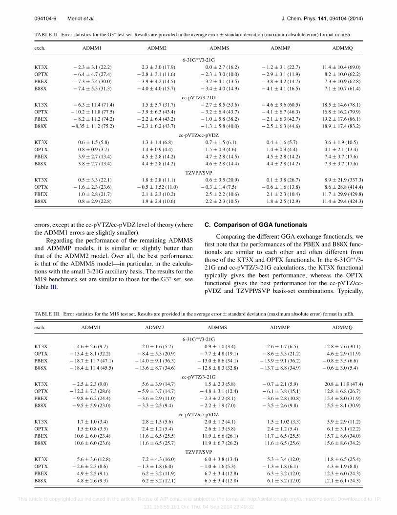
For all ADMM schemes considered here, we have per-formed calculations with four primary–auxiliary basis com-binations (6-31G∗∗/3-21G, cc-pVTZ/3-21G, cc-pVTZ/cc-pVDZ, and TZVPP/SVP) and four GGA exchange correc-tions (B88,70 PBE,71 OPTX,72 and the exchange part of theKT3 functional,73 denoted by B88X, PBEX, OPTX, andKT3X, respectively). The mean errors, maximum absolute er-rors, and standard deviations for the G3∗ and M19 test sets arecontained in Tables II and III, respectively.

In Sec. III B, we compare the various ADMM modelswith one another; in Sec. III C, the various GGA function-als are compared. Based on these results, some model func-tional pairs are singled out for further analysis in Sec. III E. InSec. III F, we address the question how well a basis set correc-tion calculated using GGA functionals approximates the exactexchange basis set correction using selected models and func-tionals. In Sec. III G, we compare the ADMM timings withthe corresponding LinK timings for the valinomycine and titinmolecules, containing 168 and 392 atoms, respectively.

B. Comparison of ADMM models

Comparing the ADMM statistics for the G3∗ benchmarkset in Table II, the first observation is that ADMMQ performsworse than the other ADMM schemes, with a largest max-imum error of 430 mEh and a typical error of 10 mEh. Asdiscussed in Sec. II E, ADMMQ gives an unbalanced treat-ment of the exact and GGA exchange due to the sensitivity ofthe SCF procedure to the charge constraint parameter as dis-cussed in Subsection II E. We note that ADMMQ performsreasonably well for some combinations of basis sets and GGAfunctionals—for example, at the 6-31G∗∗/3-21G level of the-ory. However, being considerably less robust than the otherADMM schemes, ADMMQ will not be considered furtherhere.

Regarding the relative performance of the remainingADMM models, we first note that ADMM1 performs poorlyin the small 3-21G auxiliary basis, with errors as large as 78mEh using 6-31G∗∗/3-21G with OPTX. On the other hand,ADMM1 performs significantly better at the cc-pVTZ/cc-pVDZ and TZVPP/SVP levels of theory—in fact, better thanall other ADMM models in some cases. Nevertheless, in viewof the large ADMM1 errors in the 3-21G auxiliary basis, werecommend ADMM2 over ADMM1. In fact, the ADMM2largest absolute errors are half as large as the ADMM1

This article is copyrighted as indicated in the article. Reuse of AIP content is subject to the terms at: http://scitation.aip.org/termsconditions. Downloaded to IP:

131.156.59.191 On: Thu, 04 Sep 2014 23:49:32

094104-6 Merlot et al. J. Chem. Phys. 141, 094104 (2014)

TABLE II. Error statistics for the G3∗ test set. Results are provided in the average error ± standard deviation (maximum absolute error) format in mEh.

exch. ADMM1 ADMM2 ADMMS ADMMP ADMMQ

6-31G∗∗/3-21GKT3X − 2.3 ± 3.1 (22.2) 2.3 ± 3.0 (17.9) 0.0 ± 2.7 (16.2) − 1.2 ± 3.1 (22.7) 11.4 ± 10.4 (69.0)OPTX − 6.4 ± 4.7 (27.4) − 2.8 ± 3.1 (11.6) − 2.3 ± 3.0 (10.0) − 2.9 ± 3.1 (11.9) 8.2 ± 10.0 (62.2)PBEX − 7.3 ± 5.4 (30.0) − 3.9 ± 4.2 (14.5) − 3.2 ± 4.1 (13.5) − 3.8 ± 4.2 (14.7) 7.3 ± 10.9 (62.8)B88X − 7.4 ± 5.3 (31.3) − 4.0 ± 4.0 (15.7) − 3.4 ± 4.0 (14.9) − 4.1 ± 4.1 (16.5) 7.1 ± 10.7 (61.4)

cc-pVTZ/3-21GKT3X − 6.3 ± 11.4 (71.4) 1.5 ± 5.7 (31.7) − 2.7 ± 8.5 (53.6) − 4.6 ± 9.6 (60.5) 18.5 ± 14.6 (78.1)OPTX − 10.2 ± 11.8 (77.5) − 3.9 ± 6.3 (43.4) − 3.2 ± 6.4 (43.7) − 4.1 ± 6.7 (46.3) 16.8 ± 16.2 (79.9)PBEX − 8.2 ± 11.2 (74.2) − 2.2 ± 6.4 (43.2) − 1.0 ± 5.8 (38.2) − 2.1 ± 6.3 (42.7) 19.2 ± 17.6 (86.1)B88X −8.35 ± 11.2 (75.2) − 2.3 ± 6.2 (43.7) − 1.3 ± 5.8 (40.0) − 2.5 ± 6.3 (44.6) 18.9 ± 17.4 (83.2)

cc-pVTZ/cc-pVDZKT3X 0.6 ± 1.5 (5.8) 1.3 ± 1.4 (6.8) 0.7 ± 1.5 (6.1) 0.4 ± 1.6 (5.7) 3.6 ± 1.9 (10.5)OPTX 0.8 ± 0.9 (3.7) 1.4 ± 0.9 (4.4) 1.5 ± 0.9 (4.6) 1.4 ± 0.9 (4.4) 4.1 ± 2.1 (13.4)PBEX 3.9 ± 2.7 (13.4) 4.5 ± 2.8 (14.2) 4.7 ± 2.8 (14.5) 4.5 ± 2.8 (14.2) 7.4 ± 3.7 (17.6)B88X 3.8 ± 2.7 (13.4) 4.4 ± 2.8 (14.2) 4.6 ± 2.8 (14.4) 4.4 ± 2.8 (14.2) 7.3 ± 3.7 (17.6)

TZVPP/SVPKT3X 0.5 ± 3.3 (22.1) 1.8 ± 2.8 (11.1) 0.6 ± 3.5 (20.9) 0.1 ± 3.8 (26.7) 8.9 ± 21.9 (337.3)OPTX − 1.6 ± 2.3 (23.6) − 0.5 ± 1.52 (11.0) − 0.3 ± 1.4 (7.5) − 0.6 ± 1.6 (13.8) 8.6 ± 28.8 (414.4)PBEX 1.0 ± 2.8 (21.7) 2.1 ± 2.3 (10.2) 2.5 ± 2.2 (10.6) 2.1 ± 2.3 (10.4) 11.7 ± 29.9 (429.8)B88X 0.8 ± 2.9 (22.8) 1.9 ± 2.4 (10.6) 2.2 ± 2.3 (10.5) 1.8 ± 2.5 (12.9) 11.4 ± 29.4 (424.3)

errors, except at the cc-pVTZ/cc-pVDZ level of theory (wherethe ADMM1 errors are slightly smaller).

Regarding the performance of the remaining ADMMSand ADMMP models, it is similar or slightly better thanthat of the ADMM2 model. Over all, the best performanceis that of the ADMMS model—in particular, in the calcula-tions with the small 3-21G auxiliary basis. The results for theM19 benchmark set are similar to those for the G3∗ set, seeTable III.

C. Comparison of GGA functionals

Comparing the different GGA exchange functionals, wefirst note that the performances of the PBEX and B88X func-tionals are similar to each other and often different fromthose of the KT3X and OPTX functionals. In the 6-31G∗∗/3-21G and cc-pVTZ/3-21G calculations, the KT3X functionaltypically gives the best performance, whereas the OPTXfunctional gives the best performance for the cc-pVTZ/cc-pVDZ and TZVPP/SVP basis-set combinations. Typically,

TABLE III. Error statistics for the M19 test set. Results are provided in the average error ± standard deviation (maximum absolute error) format in mEh.

exch. ADMM1 ADMM2 ADMMS ADMMP ADMMQ

6-31G∗∗/3-21GKT3X − 4.6 ± 2.6 (9.7) 2.0 ± 1.6 (5.7) − 0.9 ± 1.0 (3.4) − 2.6 ± 1.7 (6.5) 12.8 ± 7.6 (30.1)OPTX − 13.4 ± 8.1 (32.2) − 8.4 ± 5.3 (20.9) − 7.7 ± 4.8 (19.1) − 8.6 ± 5.3 (21.2) 4.6 ± 2.9 (11.9)PBEX − 18.7 ± 11.7 (47.1) − 14.0 ± 9.1 (36.3) − 13.0 ± 8.6 (34.1) − 13.9 ± 9.1 (36.2) − 0.8 ± 3.5 (6.6)B88X − 18.4 ± 11.4 (45.5) − 13.6 ± 8.7 (34.6) − 12.8 ± 8.3 (32.8) − 13.7 ± 8.8 (34.9) − 0.6 ± 3.0 (5.4)

cc-pVTZ/3-21GKT3X − 2.5 ± 2.3 (9.0) 5.6 ± 3.9 (14.7) 1.5 ± 2.3 (5.8) − 0.7 ± 2.1 (5.9) 20.8 ± 11.9 (47.4)OPTX − 12.2 ± 7.3 (28.6) − 5.9 ± 3.7 (14.7) − 4.8 ± 3.1 (12.4) − 6.1 ± 3.8 (15.1) 12.8 ± 6.8 (26.7)PBEX − 9.8 ± 6.2 (24.4) − 3.6 ± 2.9 (11.0) − 2.3 ± 2.2 (8.1) − 3.6 ± 2.8 (10.8) 15.4 ± 8.0 (31.9)B88X − 9.5 ± 5.9 (23.0) − 3.3 ± 2.5 (9.4) − 2.2 ± 1.9 (7.0) − 3.5 ± 2.6 (9.8) 15.5 ± 8.1 (30.9)

cc-pVTZ/cc-pVDZKT3X 1.7 ± 1.0 (3.4) 2.8 ± 1.5 (5.6) 2.0 ± 1.2 (4.1) 1.5 ± 1.02 (3.3) 5.9 ± 2.9 (11.2)OPTX 1.5 ± 0.8 (3.5) 2.4 ± 1.2 (5.4) 2.6 ± 1.3 (5.8) 2.4 ± 1.2 (5.4) 6.1 ± 3.1 (12.2)PBEX 10.6 ± 6.0 (23.4) 11.6 ± 6.5 (25.5) 11.9 ± 6.6 (26.1) 11.7 ± 6.5 (25.5) 15.7 ± 8.6 (34.0)B88X 10.6 ± 6.0 (23.6) 11.6 ± 6.5 (25.7) 11.9 ± 6.7 (26.2) 11.6 ± 6.5 (25.6) 15.6 ± 8.6 (34.2)

TZVPP/SVPKT3X 5.6 ± 3.6 (12.8) 7.2 ± 4.3 (16.0) 6.0 ± 3.8 (13.4) 5.3 ± 3.4 (12.0) 11.8 ± 6.5 (25.4)OPTX − 2.6 ± 2.3 (8.6) − 1.3 ± 1.8 (6.0) − 1.0 ± 1.6 (5.3) − 1.3 ± 1.8 (6.1) 4.3 ± 1.9 (8.8)PBEX 4.9 ± 2.5 (9.1) 6.2 ± 3.2 (11.9) 6.7 ± 3.4 (12.8) 6.3 ± 3.2 (12.0) 12.3 ± 6.0 (24.3)B88X 4.8 ± 2.6 (9.3) 6.2 ± 3.2 (12.1) 6.5 ± 3.4 (12.8) 6.1 ± 3.2 (12.0) 12.1 ± 6.1 (24.3)

This article is copyrighted as indicated in the article. Reuse of AIP content is subject to the terms at: http://scitation.aip.org/termsconditions. Downloaded to IP:

131.156.59.191 On: Thu, 04 Sep 2014 23:49:32

094104-7 Merlot et al. J. Chem. Phys. 141, 094104 (2014)

these functionals perform better than the PBEX functional,originally used for the ADMM1 and ADMM2 calcula-tions. For ADMMS (and ADMMP), the KT3X and OPTXfunctionals seem especially advantageous. This may be ex-plained by the fact that OPTX has been optimized to repro-duce the HF exchange energy accurately, while KT3X con-sists of the OPTX expression together with some additionalterms.

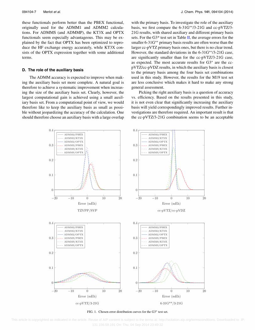
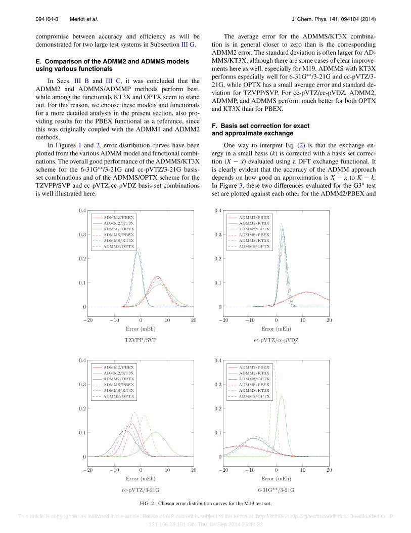
D. The role of the auxiliary basis

The ADMM accuracy is expected to improve when mak-ing the auxiliary basis set more complete. A natural goal istherefore to achieve a systematic improvement when increas-ing the size of the auxiliary basis set. Clearly, however, thelargest computational gain is achieved using a small auxil-iary basis set. From a computational point of view, we wouldtherefore like to keep the auxiliary basis as small as possi-ble without jeopardizing the accuracy of the calculation. Oneshould therefore choose an auxiliary basis with a large overlap

with the primary basis. To investigate the role of the auxiliarybasis, we first compare the 6-31G∗∗/3-21G and cc-pVTZ/3-21G results, with shared auxiliary and different primary basissets. For the G3* test set in Table II, the average errors for thesmaller 6-31G∗∗ primary basis results are often worse than thelarger cc-pVTZ primary basis ones, but there is no clear trend.However, the standard deviations in the 6-31G∗∗/3-21G case,are significantly smaller than for the cc-pVTZ/3-21G case,as expected. The most accurate results for G3∗ are the cc-pVTZ/cc-pVDZ results, in which the auxiliary basis is closestto the primary basis among the four basis set combinationsused in this study. However, the results for the M19 test setare less conclusive which makes it hard to make any stronggeneral assessment.

Picking the right auxiliary basis is a question of accuracyvs. efficiency. Based on the results presented in this study,it is not even clear that significantly increasing the auxiliarybasis will yield correspondingly improved results. Further in-vestigations are therefore required. An important result is thatthe cc-pVTZ/3-21G combination seems to be an acceptable

−20 −10 0 10 20

0

0.1

0.2

0.3

0.4

Error (mEh)

TZVPP/SVP

ADMM2/PBEX

ADMM2/KT3X

ADMM2/OPTX

ADMMS/PBEX

ADMMS/KT3X

ADMMS/OPTX

−20 −10 0 10 20

0

0.1

0.2

0.3

0.4

Error (mEh)

cc-pVTZ/cc-pVDZ

ADMM2/PBEX

ADMM2/KT3X

ADMM2/OPTX

ADMMS/PBEX

ADMMS/KT3X

ADMMS/OPTX

−20 −10 0 10 20

0

0.1

0.2

0.3

0.4

Error (mEh)

cc-pVTZ/3-21G

ADMM2/PBEX

ADMM2/KT3X

ADMM2/OPTX

ADMMS/PBEX

ADMMS/KT3X

ADMMS/OPTX

−20 −10 0 10 20

0

0.1

0.2

0.3

0.4

Error (mEh)

6-31G**/3-21G

ADMM2/PBEX

ADMM2/KT3X

ADMM2/OPTX

ADMMS/PBEX

ADMMS/KT3X

ADMMS/OPTX

FIG. 1. Chosen error distribution curves for the G3∗ test set.

This article is copyrighted as indicated in the article. Reuse of AIP content is subject to the terms at: http://scitation.aip.org/termsconditions. Downloaded to IP:

131.156.59.191 On: Thu, 04 Sep 2014 23:49:32

094104-8 Merlot et al. J. Chem. Phys. 141, 094104 (2014)

compromise between accuracy and efficiency as will bedemonstrated for two large test systems in Subsection III G.

E. Comparison of the ADMM2 and ADMMS modelsusing various functionals

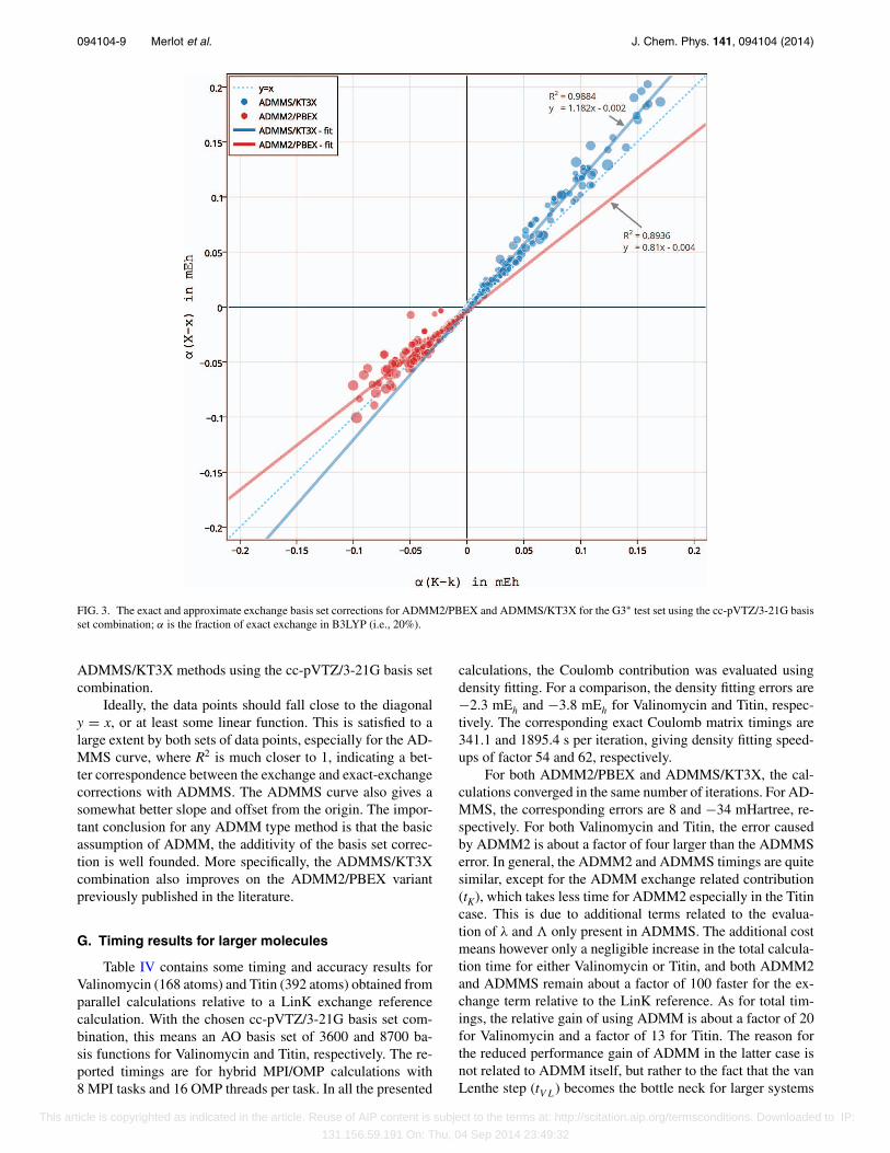
In Secs. III B and III C, it was concluded that theADMM2 and ADMMS/ADMMP methods perform best,while among the functionals KT3X and OPTX seem to standout. For this reason, we choose these models and functionalsfor a more detailed analysis in the present section, also pro-viding results for the PBEX functional as a reference, sincethis was originally coupled with the ADMM1 and ADMM2methods.

In Figures 1 and 2, error distribution curves have beenplotted from the various ADMM model and functional combi-nations. The overall good performance of the ADMMS/KT3Xscheme for the 6-31G∗∗/3-21G and cc-pVTZ/3-21G basis-set combinations and of the ADMMS/OPTX scheme for theTZVPP/SVP and cc-pVTZ-cc-pVDZ basis-set combinationsis well illustrated here.

The average error for the ADMMS/KT3X combina-tion is in general closer to zero than is the correspondingADMM2 error. The standard deviation is often larger for AD-MMS/KT3X, although there are some cases of clear improve-ments here as well, especially for M19. ADMMS with KT3Xperforms especially well for 6-31G∗∗/3-21G and cc-pVTZ/3-21G, while OPTX has a small average error and standard de-viation for TZVPP/SVP. For cc-pVTZ/cc-pVDZ, ADMM2,ADMMP, and ADMMS perform much better for both OPTXand KT3X than for PBEX.

F. Basis set correction for exactand approximate exchange

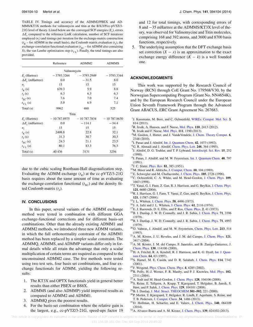
One way to interpret Eq. (2) is that the exchange en-ergy in a small basis (k) is corrected with a basis set correc-tion (X − x) evaluated using a DFT exchange functional. Itis clearly evident that the accuracy of the ADMM approachdepends on how good an approximation is X − x to K − k.In Figure 3, these two differences evaluated for the G3∗ testset are plotted against each other for the ADMM2/PBEX and

−20 −10 0 10 20

0

0.1

0.2

0.3

0.4

Error (mEh)

TZVPP/SVP

ADMM2/PBEX

ADMM2/KT3X

ADMM2/OPTX

ADMMS/PBEX

ADMMS/KT3X

ADMMS/OPTX

−20 −10 0 10 20

0

0.1

0.2

0.3

0.4

Error (mEh)

cc-pVTZ/cc-pVDZ

ADMM2/PBEX

ADMM2/KT3X

ADMM2/OPTX

ADMMS/PBEX

ADMMS/KT3X

ADMMS/OPTX

−20 −10 0 10 20

0

0.1

0.2

0.3

0.4

Error (mEh)

cc-pVTZ/3-21G

ADMM2/PBEX

ADMM2/KT3X

ADMM2/OPTX

ADMMS/PBEX

ADMMS/KT3X

ADMMS/OPTX

−20 −10 0 10 20

0

0.1

0.2

0.3

0.4

Error (mEh)

6-31G**/3-21G

ADMM2/PBEX

ADMM2/KT3X

ADMM2/OPTX

ADMMS/PBEX

ADMMS/KT3X

ADMMS/OPTX

FIG. 2. Chosen error distribution curves for the M19 test set.

This article is copyrighted as indicated in the article. Reuse of AIP content is subject to the terms at: http://scitation.aip.org/termsconditions. Downloaded to IP:

131.156.59.191 On: Thu, 04 Sep 2014 23:49:32

094104-9 Merlot et al. J. Chem. Phys. 141, 094104 (2014)

FIG. 3. The exact and approximate exchange basis set corrections for ADMM2/PBEX and ADMMS/KT3X for the G3∗ test set using the cc-pVTZ/3-21G basisset combination; α is the fraction of exact exchange in B3LYP (i.e., 20%).

ADMMS/KT3X methods using the cc-pVTZ/3-21G basis setcombination.

Ideally, the data points should fall close to the diagonaly = x, or at least some linear function. This is satisfied to alarge extent by both sets of data points, especially for the AD-MMS curve, where R2 is much closer to 1, indicating a bet-ter correspondence between the exchange and exact-exchangecorrections with ADMMS. The ADMMS curve also gives asomewhat better slope and offset from the origin. The impor-tant conclusion for any ADMM type method is that the basicassumption of ADMM, the additivity of the basis set correc-tion is well founded. More specifically, the ADMMS/KT3Xcombination also improves on the ADMM2/PBEX variantpreviously published in the literature.

G. Timing results for larger molecules

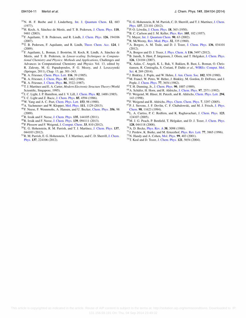
Table IV contains some timing and accuracy results forValinomycin (168 atoms) and Titin (392 atoms) obtained fromparallel calculations relative to a LinK exchange referencecalculation. With the chosen cc-pVTZ/3-21G basis set com-bination, this means an AO basis set of 3600 and 8700 ba-sis functions for Valinomycin and Titin, respectively. The re-ported timings are for hybrid MPI/OMP calculations with8 MPI tasks and 16 OMP threads per task. In all the presented

calculations, the Coulomb contribution was evaluated usingdensity fitting. For a comparison, the density fitting errors are−2.3 mEh and −3.8 mEh for Valinomycin and Titin, respec-tively. The corresponding exact Coulomb matrix timings are341.1 and 1895.4 s per iteration, giving density fitting speed-ups of factor 54 and 62, respectively.

For both ADMM2/PBEX and ADMMS/KT3X, the cal-culations converged in the same number of iterations. For AD-MMS, the corresponding errors are 8 and −34 mHartree, re-spectively. For both Valinomycin and Titin, the error causedby ADMM2 is about a factor of four larger than the ADMMSerror. In general, the ADMM2 and ADMMS timings are quitesimilar, except for the ADMM exchange related contribution(tK), which takes less time for ADMM2 especially in the Titincase. This is due to additional terms related to the evalua-tion of λ and � only present in ADMMS. The additional costmeans however only a negligible increase in the total calcula-tion time for either Valinomycin or Titin, and both ADMM2and ADMMS remain about a factor of 100 faster for the ex-change term relative to the LinK reference. As for total tim-ings, the relative gain of using ADMM is about a factor of 20for Valinomycin and a factor of 13 for Titin. The reason forthe reduced performance gain of ADMM in the latter case isnot related to ADMM itself, but rather to the fact that the vanLenthe step (tV L) becomes the bottle neck for larger systems

This article is copyrighted as indicated in the article. Reuse of AIP content is subject to the terms at: http://scitation.aip.org/termsconditions. Downloaded to IP:

131.156.59.191 On: Thu, 04 Sep 2014 23:49:32

094104-10 Merlot et al. J. Chem. Phys. 141, 094104 (2014)

TABLE IV. Timings and accuracy of the ADMM2/PBEX and AD-MMS/KT3X methods for valinomycin and titin at the B3LYP/cc-pVTZ/3-21G level of theory. Listed below are the converged SCF energies (Et), errors�Et compared to the reference LinK calculation, number of SCF iterationsemployed (ni) and timings per iteration for the exchange-matrix construction(tK – for ADMM in the small basis), the Coulomb matrix evaluation (tJ), theexchange-correlation functional evaluation (tXC – for ADMM also containingX), the van Lenthe optimization step (t

V L). Finally, the total timings are also

provided.

Reference ADMM2 ADMMS

ValinomycinEt (Hartree) − 3793.3264 − 3793.2949 − 3793.3344�Et (mHartree) 0.0 − 31.5 8.0ni 15 15 15tK (s) 639.3 5.9 8.8tJ (s) 6.3 6.3 6.3tXC (s) 7.6 7.0 7.4tV L

(s) 5.9 6.9 7.1

Total (s) 9962 460 525

TitinEt (Hartree) − 10 787.8975 − 10 787.7834 − 10 787.8630�Et (mHartree) 0.0 − 114.1 − 34.4ni 15 15 15tK (s) 2498.8 22.8 32.1tJ (s) 31.3 30.7 30.3tXC (s) 24.3 21.1 23.5tV L

(s) 80.1 83.3 76.3

Total (s) 40 436 3131 3256

due to the cubic scaling Roothaan-Hall diagonalization step.Evaluating the ADMM exchange (tK) at the cc-pVTZ/3-21Gbasis requires about the same amount of time as evaluatingthe exchange-correlation functional (tXC) and the density fit-ted Coulomb matrix (tJ).

IV. CONCLUSIONS

In this paper, several variants of the ADMM exchangemethod were tested in combination with different GGAexchange-functional corrections and for different basis-setcombinations. Other than the already existing ADMM1 andADMM2 methods, we introduced three new ADMM variants,in which the full orthonormality constraint of the ADMM1method has been replaced by a simpler scalar constraint. TheADMMQ, ADMMS, and ADMMP variants differ only in for-mal details while all retain the advantage that only a scalarmultiplication of certain terms are required as compared to theunconstrained ADMM2 case. The five methods were testedusing two test sets, four basis set combinations, and four ex-change functionals for ADMM, yielding the following re-sults:

1. The KT3X and OPTX functionals yield in general betterresults than either PBEX or B88X.

2. ADMMS (and also ADMMP) yield improved results ascompared to ADMM2 and ADMM1.

3. ADMMQ gives the poorest results.4. For the basis-set combination where the relative gain is

the largest, e.g., cc-pVTZ/3-21G, speed-ups factor 19

and 12 for total timings, with corresponding errors of8 and −35 mHartree at the ADMMS/KT3X level of the-ory, was observed for Valinomycine and Titin molecules,comprising 168 and 392 atoms, and 3600 and 8700 basisfunctions, respectively.

5. The underlying assumption that the DFT exchange basisset correction (X − x) is an approximation to the exactexchange energy difference (K − k) is a well foundedone.

ACKNOWLEDGMENTS

This work was supported by the Research Council ofNorway (RCN) through CoE Grant No. 179568/V30, by theNorwegian Supercomputing Program (Grant No. NN4654K),and by the European Research Council under the EuropeanUnion Seventh Framework Program through the AdvancedGrant ABACUS, ERC Grant Agreement No. 267683.

1J. Kussmann, M. Beer, and C. Ochsenfeld, WIREs: Comput. Mol. Sci. 3,614 (2013).

2R. Izsák, A. Hansen, and F. Neese, Mol. Phys. 110, 2413 (2012).3R. Izsák and F. Neese, Mol. Phys. 111, 1190 (2013).4M. Guidon, J. Hutter, and J. VandeVondele, J. Chem. Theory Comput. 6,2348 (2010).

5I. Panas and J. Almlöf, Int. J. Quantum Chem. 42, 1073 (1992).6G. R. Ahmadi and J. Almlöf, Chem. Phys. Lett. 246, 364 (1995).7J. Almlöf, D. G. Truhlar, and T. P. Lybrand, Interdiscipl. Sci. Rev. 15, 252(1990).

8I. Panas, J. Almlöf, and M. W. Feyereisen, Int. J. Quantum Chem. 40, 797(1991).

9J. C. Slater, Phys. Rev. 81, 385 (1951).10M. Häser and R. Ahlrichs, J. Comput. Chem. 10, 104 (1989).11E. Schwegler and M. Challacombe, J. Chem. Phys. 105, 2726 (1996).12C. Ochsenfeld, C. A. White, and M. Head-Gordon, J. Chem. Phys. 109,

1663 (1998).13T. Yanai, G. I. Fann, Z. Gan, R. J. Harrison, and G. Beylkin, J. Chem. Phys.

121, 6680 (2004).14R. J. Harrison, G. I. Fann, T. Yanai, Z. Gan, and G. Beylkin, J. Chem. Phys.

121, 11587 (2004).15J. L. Whitten, J. Chem. Phys. 58, 4496 (1973).16J. A. Jafri and J. L. Whitten, J. Chem. Phys. 61, 2116 (1974).17E. J. Baerends, D. E. Ellis, and P. Ros, Chem. Phys. 2, 41 (1973).18B. I. Dunlap, J. W. D. Connolly, and J. R. Sabin, J. Chem. Phys. 71, 3396

(1979).19B. I. Dunlap, J. W. D. Connolly, and J. R. Sabin, J. Chem. Phys. 71, 4993

(1979).20O. Vahtras, J. Almlöf, and M. W. Feyereisen, Chem. Phys. Lett. 213, 514

(1993).21A. M. Köster, J. U. Reveles, and J. M. del Campo, J. Chem. Phys. 121,

3417 (2004).22A. M. Köster, J. M. del Campo, F. Janetzko, and B. Zuniga-Gutierrez, J.

Chem. Phys. 130, 114106 (2009).23H. A. Früchtl, R. A. Kendall, R. J. Harrison, and K. G. Dyall, Int. J. Quan-

tum Chem. 64, 63 (1997).24S. Hamel, M. E. Casida, and D. R. Salahub, J. Chem. Phys. 114, 7342

(2001).25F. Weigend, Phys. Chem. Chem. Phys. 4, 4285 (2002).26R. Polly, H.-J. Werner, F. R. Manby, and P. J. Knowles, Mol. Phys. 102,

2311 (2004).27A. Sodt and M. Head-Gordon, J. Chem. Phys. 128, 104106 (2008).28S. Reine, E. Tellgren, A. Krapp, T. Kjærgaard, T. Helgaker, B. Jansík, S.

Høst, and P. Sałek, J. Chem. Phys. 129, 104101 (2008).29B. I. Dunlap, J. Mol. Struct. THEOCHEM 501–502, 221 (2000).30P. Merlot, T. Kjærgaard, T. Helgaker, R. Lindh, F. Aquilante, S. Reine, and

T. B. Pedersen, J. Comput. Chem. 34, 1486 (2013).31D. Hollman, H. Schaefer, and E. Valeev, J. Chem. Phys. 140, 064109

(2014).32A. Alvarez-Ibarra and A. M. Köster, J. Chem. Phys. 139, 024102 (2013).

This article is copyrighted as indicated in the article. Reuse of AIP content is subject to the terms at: http://scitation.aip.org/termsconditions. Downloaded to IP:

131.156.59.191 On: Thu, 04 Sep 2014 23:49:32

094104-11 Merlot et al. J. Chem. Phys. 141, 094104 (2014)

33N. H. F. Beebe and J. Linderberg, Int. J. Quantum Chem. 12, 683(1977).

34H. Koch, A. Sánchez de Merás, and T. B. Pedersen, J. Chem. Phys. 118,9481 (2003).

35F. Aquilante, T. B. Pedersen, and R. Lindh, J. Chem. Phys. 126, 194106(2007).

36T. B. Pedersen, F. Aquilante, and R. Lindh, Theor. Chem. Acc. 124, 1(2009).

37F. Aquilante, L. Boman, J. Boström, H. Koch, R. Lindh, A. Sánchez deMerás, and T. B. Pedersen, in Linear-scaling Techniques in Computa-tional Chemistry and Physics: Methods and Applications, Challenges andAdvances in Computational Chemistry and Physics Vol. 13, edited byR. Zalesny, M. G. Papadopoulos, P. G. Mezey, and J. Leszczynski(Springer, 2011), Chap. 13, pp. 301–343.

38R. A. Friesner, Chem. Phys. Lett. 116, 39 (1985).39R. A. Friesner, J. Chem. Phys. 85, 1462 (1986).40R. A. Friesner, J. Chem. Phys. 86, 3522 (1987).41T. J. Martínez and E. A. Carter, Modern Electronic Structure Theory (World

Scientific, Singapore, 1995).42J. C. Light, I. P. Hamilton, and J. V. Lill, J. Chem. Phys. 82, 1400 (1985).43J. C. Light and Z. Bacic, J. Chem. Phys. 85, 4594 (1986).44W. Yang and A. C. Peet, Chem. Phys. Lett. 153, 98 (1988).45A. Yachmenev and W. Klopper, Mol. Phys. 111, 1129 (2013).46F. Neese, F. Wennmohs, A. Hansen, and U. Becker, Chem. Phys. 356, 98

(2009).47R. Izsák and F. Neese, J. Chem. Phys. 135, 144105 (2011).48R. Izsák and F. Neese, J. Chem. Phys. 139, 094111 (2013).49P. Plessow and F. Weigend, J. Comput. Chem. 33, 810 (2012).50E. G. Hohenstein, R. M. Parrish, and T. J. Martínez, J. Chem. Phys. 137,

044103 (2012).51R. M. Parrish, E. G. Hohenstein, T. J. Martínez, and C. D. Sherrill, J. Chem.

Phys. 137, 224106 (2012).

52E. G. Hohenstein, R. M. Parrish, C. D. Sherrill, and T. J. Martínez, J. Chem.Phys. 137, 221101 (2012).

53P.-O. Löwdin, J. Chem. Phys. 18, 365 (1950).54B. C. Carlson and J. M. Keller, Phys. Rev. 105, 102 (1957).55I. Mayer, Int. J. Quantum Chem. 90, 63 (2002).56R. McWeeny, Rev. Mod. Phys. 32, 335 (1960).57A. Borgoo, A. M. Teale, and D. J. Tozer, J. Chem. Phys. 136, 034101

(2012).58A. Borgoo and D. J. Tozer, J. Phys. Chem. A 116, 5497 (2012).59B. Jansík, S. Høst, P. Jørgensen, J. Olsen, and T. Helgaker, J. Chem. Phys.

126, 124104 (2007).60K. Aidas, C. Angeli, K. L. Bak, V. Bakken, R. Bast, L. Boman, O. Chris-

tiansen, R. Cimiraglia, S. Coriani, P. Dahle et al., WIREs: Comput. Mol.Sci. 4, 269 (2014).

61J. Binkley, J. Pople, and W. Hehre, J. Am. Chem. Soc. 102, 939 (1980).62M. Francl, W. Petro, W. Hehre, J. Binkley, M. Gordon, D. DeFrees, and J.

Pople, J. Chem. Phys. 77, 3654 (1982).63T. H. Dunning, Jr., J. Chem. Phys. 90, 1007 (1989).64A. Schäfer, H. Horn, and R. Ahlrichs, J. Chem. Phys. 97, 2571 (1992).65F. Weigend, M. Häser, H. Patzelt, and R. Ahlrichs, Chem. Phys. Lett. 294,

143 (1998).66F. Weigend and R. Ahlrichs, Phys. Chem. Chem. Phys. 7, 3297 (2005).67P. J. Stevens, J. F. Devlin, C. F. Chabalowski, and M. J. Frisch, J. Phys.

Chem. 98, 11623 (1994).68L. A. Curtiss, P. C. Redfern, and K. Raghavachari, J. Chem. Phys. 123,

124107 (2005).69M. J. G. Peach, P. Benfield, T. Helgaker, and D. J. Tozer, J. Chem. Phys.

128, 044118 (2008).70A. D. Becke, Phys. Rev. A 38, 3098 (1988).71J. Perdew, K. Burke, and M. Ernzerhof, Phys. Rev. Lett. 77, 3865 (1996).72N. Handy and A. Cohen, Mol. Phys. 99, 403 (2001).73T. Keal and D. Tozer, J. Chem. Phys. 121, 5654 (2004).

This article is copyrighted as indicated in the article. Reuse of AIP content is subject to the terms at: http://scitation.aip.org/termsconditions. Downloaded to IP:

131.156.59.191 On: Thu, 04 Sep 2014 23:49:32