Characterizing the distinctive acoustic cues of Mandarin tones

Characterizing the distinctive acoustic cues of Mandarin tones

Paul Tupper,1,a) Keith Leung,2 Yue Wang,2 Allard Jongman,3 and Joan A. Sereno3

1Department of Mathematics, Simon Fraser University, Burnaby, British Colombia V5A 1S6, Canada2Department of Linguistics, Simon Fraser University, Burnaby, British Colombia V5A 1S6, Canada3Department of Linguistics, University of Kansas, Lawrence, Kansas 66045, USA

ABSTRACT:This study aims to characterize distinctive acoustic features of Mandarin tones based on a corpus of 1025

monosyllabic words produced by 21 native Mandarin speakers. For each tone, 22 acoustic cues were extracted.

Besides standard F0, duration, and intensity measures, further cues were determined by fitting two mathematical

functions to the pitch contours. The first function is a parabola, which gives three parameters: a mean F0, an F0

slope, and an F0 second derivative. The second is a broken-line function, which models the contour as a continuous

curve consisting of two lines with a single breakpoint. Cohen’s d, sparse Principal Component Analysis, and other

statistical measures are used to identify which of the cues, and which combinations of the cues, are important for

distinguishing each tone from each other among all the speakers. Although the specific cues that best characterize

the tone contours depend on the particular tone and the statistical measure used, this paper shows that the three cues

obtained by fitting a parabola to the tone contour are broadly effective. This research suggests using these three cues

as a canonical choice for defining tone characteristics. VC 2020 Acoustical Society of America.

https://doi.org/10.1121/10.0001024

(Received 21 October 2019; revised 10 February 2020; accepted 18 March 2020; published online 24 April 2020)

[Editor: Anders Lofqvist] Pages: 2570–2580

I. INTRODUCTION

Many languages, including Mandarin Chinese, employ

tones to convey lexical meaning. Acoustically, lexical tones

are manifested primarily as changes in fundamental fre-

quency (F0, perceived as pitch) as well as duration and

amplitude (Howie and Howie, 1976; Lehiste, 1970).

However, the critical acoustic cues characterizing individual

tones had not been consistently identified in previous

research. A difficulty of this type of investigation is that a

tone contour is how F0 varies as a function of time for the

whole voiced portion of the signal. It is an example of

infinite-dimensional (or functional) data in that, to perfectly

describe the contour, one needs to record F0 at every instant

in time. In practice, of course, this is impractical and unnec-

essary. It is possible to summarize the tone contours with a

small number of cues, as many authors have done (e.g.,

Barry and Blamey, 2004; Hirst and Espesser, 1993; Wong

et al., 2017; Yang, 2015). This raises the question of which

set of cues are the most informative for describing the tone

contours of Mandarin. The current study considers a wide

selection of cues, some occurring in the literature and some

new ones, and uses a large corpus of spoken words in

Mandarin to assess which cues are the most successful in

distinguishing different tones.

There is a long history of using cues to study the tones

of Mandarin. Much of the early work was based on percep-

tual data, using artificially generated tones and studying

listeners’ discrimination judgements. An important early

investigation (Gandour, 1983) used a multi-dimensional

scaling technique (INDSCAL: individual difference scaling;

Carroll and Chang, 1970) on dissimilarity judgements to

place a selection of tone contours in a two-dimensional

space. This space can be thought of as the perceptual space

of the listeners when presented with tone stimuli. The nature

of multi-dimensional scaling techniques in general is that

they do not provide an explicit map that can then be used to

compute cues for new stimuli. But Gandour analyzed the

two dimensions provided by INDSCAL and determined that

they are roughly what he calls “height” and “direction.” His

“height” is average or mean F0 for each tone, and his

“direction” appears to correspond to slope of the F0 contour

for each tone, though perhaps slope toward the end of the

contour is more accurate.

Acoustic studies have also identified F0 mean and slope

as critical tonal cues. For example, Wong et al. (2017) used

five F0 height measurements (mean, initial, final, maximum,

and minimum) as well as a direction measure (the slope of

the second half of the F0 contour) to characterize Cantonese

tones. The second half of the syllable was selected based on

the previous findings that perceptual cues for tones are car-

ried toward the end of the syllable (Khouw and Ciocca,

2007; Xu, 2001; Xu and Wang, 2001).

Based on Gandour (1983) and other studies, a reason-

able pair of cues to describe tone contours are F0 mean and

slope. Mean is straightforwardly defined as the mean F0

over the duration of the periodic portion. However, there are

a few different ways of defining the “slope” or “direction”a)Electronic mail: [email protected]

2570 J. Acoust. Soc. Am. 147 (4), April 2020 VC 2020 Acoustical Society of America0001-4966/2020/147(4)/2570/11/$30.00

ARTICLE...................................

of a tone contour. Let us assume that we normalize our tone

contours so that they are all the same duration in time, say, 1

time unit. Some authors (e.g., Yang, 2015) use the differ-

ence between F0 at offset and F0 at onset, which, if the con-

tour were a straight line, would yield its slope (since we are

assuming a time duration of 1). Another option is to take the

range of F0 values and divide by the duration (Flemming

and Cho, 2017; Jeng et al., 2006). This always gives a posi-

tive value and, if applied to a straight line, gives the absolute

value of the slope. However, this measurement fails to dif-

ferentiate between a falling tone and a rising tone with the

same amplitude of slope. A more sophisticated method,

which relies on the entire tone contour rather than just a pair

of distinguished points, is to fit a linear function to the con-

tour in the least-squares sense (e.g., Black and Hunt, 1996;

Ghosh and Narayanan, 2009; Hirst and Espesser, 1993).

This is a special case of least-squares fitting. More gener-

ally, the fundamental idea of least-squares fitting is to select

a model with unknown coefficients (such as height and

slope, in this case) and then choose the coefficients so that

the integrated squared difference between the model and the

data is minimized. We will use this method to compute our

slope cue, as we describe later.

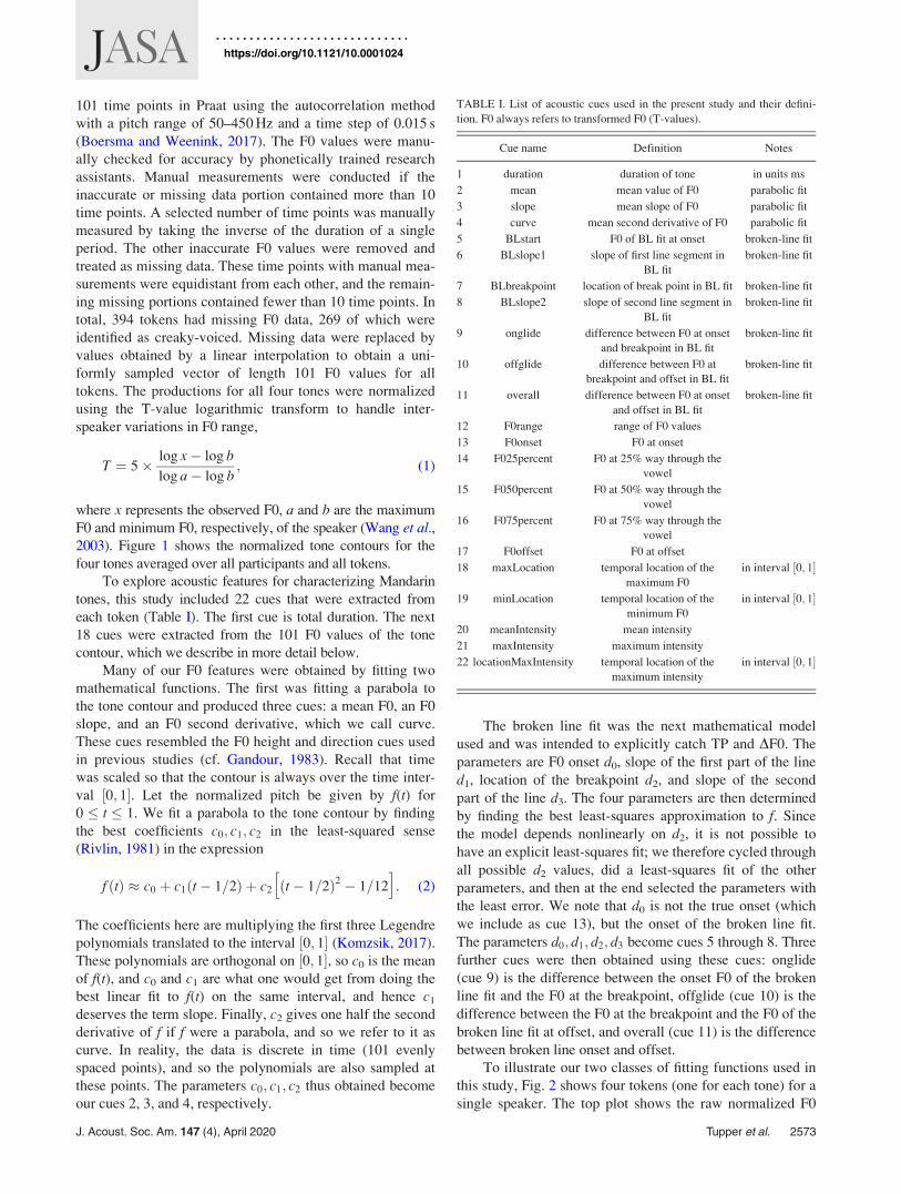
The problem with just using mean and slope to charac-

terize tone contours is that they do not capture what is one

of the most salient features of some tone contours: their

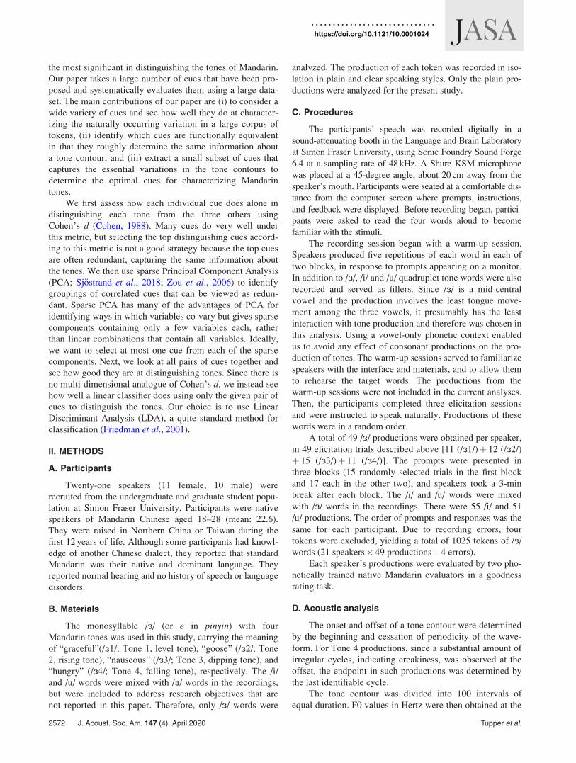
curvature. For example, Tone 3 of Mandarin starts high,

dips down, and returns to nearly the same height (see

Fig. 1). But slope computed by any of the above methods is

nearly zero. If mean and slope were the only cues that were

used, a Tone 3 would be indistinguishable from a Tone 1

produced at an overall lower pitch. As we will show, it is

necessary to introduce at least one additional cue to capture

important variations among the tone contours. We do this by

fitting a parabola to tone contours, which gives three cues

corresponding to mean, slope, and second derivative,

respectively. Other authors who have fit a parabola to

extract cues include Chen et al. (2017); Li and Chen (2016);

Shih and Lu (2015); Zhang and Meng (2016).

Other studies have found additional dynamic and local

cues to be important. Smith and Burnham (2012) included

18 F0-related acoustic cues to Mandarin tones, finding mean

and minimum F0 velocity as well as F0 onset to be critical

cues to auditory tone perception. Similarly, Barry and

Blamey (2004) used F0 offset and F0 onset to study tone dif-

ferentiation in Cantonese. Another approach is to construct

a model of how F0 contours arise from more basic phenom-

ena (Prom-on et al., 2012; Prom-on et al., 2009; Xu, 2005;

Xu and Wang, 2001). The motivation of these authors is

mainly coarticulation in polysyllabic speech.

Another cue that has been proposed based on perception

studies is turning point location (TP), defined as the tempo-

ral interval between the onset and the lowest point of the

contour (Moore and Jongman, 1997; Zhao and Kuhl, 2015).

Moore and Jongman parametrized tone contours with TP

and DF0, which was defined as the drop in F0 from onset to

the turning point. TP is likely to be useful for distinguishing

Tone 2 from Tone 3. We capture turning point (and many

other cues) using a broken line fit. We define a broken line

to be a continuous function over a time interval that consists

of two straight lines with a single breakpoint. It is described

by four parameters. One of these, the breakpoint, which

gives the location of the breakpoint in the interval, corre-

sponds to the turning point in these earlier studies.

Previous studies found that the temporal envelope cues

are pertinent to tone perception (Fu and Zeng, 2000; Fu

et al., 1998; Kong and Zeng, 2006; Wang et al., 2011).

Temporal envelope cues include three main acoustic cues:

periodicity, amplitude contour, and duration (Fu and Zeng,

2000; Kong and Zeng, 2006; Rosen, 1992). Among these

cues, periodicity reflects F0 in the speech signal (Rosen,

1992) and is covered by the above-mentioned F0 acoustic

cues. As for amplitude, when Mandarin listeners perceive

Mandarin monosyllabic stimuli without F0 or formant infor-

mation, the amplitude contour becomes a useful cue in the

perception of Mandarin Tone 2, Tone 3, and Tone 4 (Fu and

Zeng, 2000; Whalen and Xu, 1992). Acoustic studies consis-

tently show that the intrinsic amplitude varies across tones,

with Tone 3 having the lowest, and Tone 4 the highest over-

all amplitude (Chuang et al., 1972). Duration is used for

perceiving whispered speech (Liu and Samuel, 2004). When

F0 information is present, the modifying duration of stimuli

can shift the perceptual boundary between Tone 2 and Tone

3 in native and non-native speakers (Blicher et al., 1990).

Accordingly, in our study we include duration as a cue, as

well as three cues related to amplitude.

In all the work we have surveyed here, only a few dif-

ferent cues are considered, which are either extracted from

data using multidimensional scaling (Gandour, 1983), or

postulated by the researchers based on inspection of the data

and basic knowledge of how the Mandarin tone system

works. Seldom are different cues compared to see which are

FIG. 1. (Color online) The four Mandarin tones as computed from our data.

All tone contours were normalized to have the same duration, and the F0

values were log-transformed. Here we show these transformed tone con-

tours averaged over all speakers and all tokens for each of the four tones.

J. Acoust. Soc. Am. 147 (4), April 2020 Tupper et al. 2571

https://doi.org/10.1121/10.0001024

the most significant in distinguishing the tones of Mandarin.

Our paper takes a large number of cues that have been pro-

posed and systematically evaluates them using a large data-

set. The main contributions of our paper are (i) to consider a

wide variety of cues and see how well they do at character-

izing the naturally occurring variation in a large corpus of

tokens, (ii) identify which cues are functionally equivalent

in that they roughly determine the same information about

a tone contour, and (iii) extract a small subset of cues that

captures the essential variations in the tone contours to

determine the optimal cues for characterizing Mandarin

tones.

We first assess how each individual cue does alone in

distinguishing each tone from the three others using

Cohen’s d (Cohen, 1988). Many cues do very well under

this metric, but selecting the top distinguishing cues accord-

ing to this metric is not a good strategy because the top cues

are often redundant, capturing the same information about

the tones. We then use sparse Principal Component Analysis

(PCA; Sj€ostrand et al., 2018; Zou et al., 2006) to identify

groupings of correlated cues that can be viewed as redun-

dant. Sparse PCA has many of the advantages of PCA for

identifying ways in which variables co-vary but gives sparse

components containing only a few variables each, rather

than linear combinations that contain all variables. Ideally,

we want to select at most one cue from each of the sparse

components. Next, we look at all pairs of cues together and

see how good they are at distinguishing tones. Since there is

no multi-dimensional analogue of Cohen’s d, we instead see

how well a linear classifier does using only the given pair of

cues to distinguish the tones. Our choice is to use Linear

Discriminant Analysis (LDA), a quite standard method for

classification (Friedman et al., 2001).

II. METHODS

A. Participants

Twenty-one speakers (11 female, 10 male) were

recruited from the undergraduate and graduate student popu-

lation at Simon Fraser University. Participants were native

speakers of Mandarin Chinese aged 18–28 (mean: 22.6).

They were raised in Northern China or Taiwan during the

first 12 years of life. Although some participants had knowl-

edge of another Chinese dialect, they reported that standard

Mandarin was their native and dominant language. They

reported normal hearing and no history of speech or language

disorders.

B. Materials

The monosyllable /˘/ (or e in pinyin) with four

Mandarin tones was used in this study, carrying the meaning

of “graceful”(/˘1/; Tone 1, level tone), “goose” (/˘2/; Tone

2, rising tone), “nauseous” (/˘3/; Tone 3, dipping tone), and

“hungry” (/˘4/; Tone 4, falling tone), respectively. The /i/

and /u/ words were mixed with /˘/ words in the recordings,

but were included to address research objectives that are

not reported in this paper. Therefore, only /˘/ words were

analyzed. The production of each token was recorded in iso-

lation in plain and clear speaking styles. Only the plain pro-

ductions were analyzed for the present study.

C. Procedures

The participants’ speech was recorded digitally in a

sound-attenuating booth in the Language and Brain Laboratory

at Simon Fraser University, using Sonic Foundry Sound Forge

6.4 at a sampling rate of 48 kHz. A Shure KSM microphone

was placed at a 45-degree angle, about 20 cm away from the

speaker’s mouth. Participants were seated at a comfortable dis-

tance from the computer screen where prompts, instructions,

and feedback were displayed. Before recording began, partici-

pants were asked to read the four words aloud to become

familiar with the stimuli.

The recording session began with a warm-up session.

Speakers produced five repetitions of each word in each of

two blocks, in response to prompts appearing on a monitor.

In addition to /˘/, /i/ and /u/ quadruplet tone words were also

recorded and served as fillers. Since /˘/ is a mid-central

vowel and the production involves the least tongue move-

ment among the three vowels, it presumably has the least

interaction with tone production and therefore was chosen in

this analysis. Using a vowel-only phonetic context enabled

us to avoid any effect of consonant productions on the pro-

duction of tones. The warm-up sessions served to familiarize

speakers with the interface and materials, and to allow them

to rehearse the target words. The productions from the

warm-up sessions were not included in the current analyses.

Then, the participants completed three elicitation sessions

and were instructed to speak naturally. Productions of these

words were in a random order.

A total of 49 /˘/ productions were obtained per speaker,

in 49 elicitation trials described above [11 (/˘1/)þ 12 (/˘2/)

þ 15 (/˘3/)þ 11 (/˘4/)]. The prompts were presented in

three blocks (15 randomly selected trials in the first block

and 17 each in the other two), and speakers took a 3-min

break after each block. The /i/ and /u/ words were mixed

with /˘/ words in the recordings. There were 55 /i/ and 51

/u/ productions. The order of prompts and responses was the

same for each participant. Due to recording errors, four

tokens were excluded, yielding a total of 1025 tokens of /˘/

words (21 speakers� 49 productions – 4 errors).

Each speaker’s productions were evaluated by two pho-

netically trained native Mandarin evaluators in a goodness

rating task.

D. Acoustic analysis

The onset and offset of a tone contour were determined

by the beginning and cessation of periodicity of the wave-

form. For Tone 4 productions, since a substantial amount of

irregular cycles, indicating creakiness, was observed at the

offset, the endpoint in such productions was determined by

the last identifiable cycle.

The tone contour was divided into 100 intervals of

equal duration. F0 values in Hertz were then obtained at the

2572 J. Acoust. Soc. Am. 147 (4), April 2020 Tupper et al.

https://doi.org/10.1121/10.0001024

101 time points in Praat using the autocorrelation method

with a pitch range of 50–450 Hz and a time step of 0.015 s

(Boersma and Weenink, 2017). The F0 values were manu-

ally checked for accuracy by phonetically trained research

assistants. Manual measurements were conducted if the

inaccurate or missing data portion contained more than 10

time points. A selected number of time points was manually

measured by taking the inverse of the duration of a single

period. The other inaccurate F0 values were removed and

treated as missing data. These time points with manual mea-

surements were equidistant from each other, and the remain-

ing missing portions contained fewer than 10 time points. In

total, 394 tokens had missing F0 data, 269 of which were

identified as creaky-voiced. Missing data were replaced by

values obtained by a linear interpolation to obtain a uni-

formly sampled vector of length 101 F0 values for all

tokens. The productions for all four tones were normalized

using the T-value logarithmic transform to handle inter-

speaker variations in F0 range,

T ¼ 5� log x� log b

log a� log b; (1)

where x represents the observed F0, a and b are the maximum

F0 and minimum F0, respectively, of the speaker (Wang et al.,2003). Figure 1 shows the normalized tone contours for the

four tones averaged over all participants and all tokens.

To explore acoustic features for characterizing Mandarin

tones, this study included 22 cues that were extracted from

each token (Table I). The first cue is total duration. The next

18 cues were extracted from the 101 F0 values of the tone

contour, which we describe in more detail below.

Many of our F0 features were obtained by fitting two

mathematical functions. The first was fitting a parabola to

the tone contour and produced three cues: a mean F0, an F0

slope, and an F0 second derivative, which we call curve.

These cues resembled the F0 height and direction cues used

in previous studies (cf. Gandour, 1983). Recall that time

was scaled so that the contour is always over the time inter-

val ½0; 1�. Let the normalized pitch be given by f(t) for

0 � t � 1. We fit a parabola to the tone contour by finding

the best coefficients c0; c1; c2 in the least-squared sense

(Rivlin, 1981) in the expression

f ðtÞ � c0 þ c1ðt� 1=2Þ þ c2 ðt� 1=2Þ2 � 1=12

h i: (2)

The coefficients here are multiplying the first three Legendre

polynomials translated to the interval ½0; 1� (Komzsik, 2017).

These polynomials are orthogonal on ½0; 1�, so c0 is the mean

of f(t), and c0 and c1 are what one would get from doing the

best linear fit to f(t) on the same interval, and hence c1

deserves the term slope. Finally, c2 gives one half the second

derivative of f if f were a parabola, and so we refer to it as

curve. In reality, the data is discrete in time (101 evenly

spaced points), and so the polynomials are also sampled at

these points. The parameters c0; c1; c2 thus obtained become

our cues 2, 3, and 4, respectively.

The broken line fit was the next mathematical model

used and was intended to explicitly catch TP and DF0. The

parameters are F0 onset d0, slope of the first part of the line

d1, location of the breakpoint d2, and slope of the second

part of the line d3. The four parameters are then determined

by finding the best least-squares approximation to f. Since

the model depends nonlinearly on d2, it is not possible to

have an explicit least-squares fit; we therefore cycled through

all possible d2 values, did a least-squares fit of the other

parameters, and then at the end selected the parameters with

the least error. We note that d0 is not the true onset (which

we include as cue 13), but the onset of the broken line fit.

The parameters d0; d1; d2; d3 become cues 5 through 8. Three

further cues were then obtained using these cues: onglide

(cue 9) is the difference between the onset F0 of the broken

line fit and the F0 at the breakpoint, offglide (cue 10) is the

difference between the F0 at the breakpoint and the F0 of the

broken line fit at offset, and overall (cue 11) is the difference

between broken line onset and offset.

To illustrate our two classes of fitting functions used in

this study, Fig. 2 shows four tokens (one for each tone) for a

single speaker. The top plot shows the raw normalized F0

TABLE I. List of acoustic cues used in the present study and their defini-

tion. F0 always refers to transformed F0 (T-values).

Cue name Definition Notes

1 duration duration of tone in units ms

2 mean mean value of F0 parabolic fit

3 slope mean slope of F0 parabolic fit

4 curve mean second derivative of F0 parabolic fit

5 BLstart F0 of BL fit at onset broken-line fit

6 BLslope1 slope of first line segment in

BL fit

broken-line fit

7 BLbreakpoint location of break point in BL fit broken-line fit

8 BLslope2 slope of second line segment in

BL fit

broken-line fit

9 onglide difference between F0 at onset

and breakpoint in BL fit

broken-line fit

10 offglide difference between F0 at

breakpoint and offset in BL fit

broken-line fit

11 overall difference between F0 at onset

and offset in BL fit

broken-line fit

12 F0range range of F0 values

13 F0onset F0 at onset

14 F025percent F0 at 25% way through the

vowel


vowel


vowel

17 F0offset F0 at offset

18 maxLocation temporal location of the

maximum F0

in interval ½0; 1�

19 minLocation temporal location of the

minimum F0


20 meanIntensity mean intensity

21 maxIntensity maximum intensity

22 locationMaxIntensity temporal location of the

maximum intensity



https://doi.org/10.1121/10.0001024

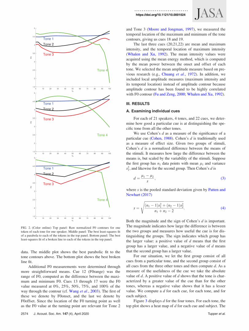
data. The middle plot shows the best parabolic fit to the

tone contours above. The bottom plot shows the best broken

line fit.

Additional F0 measurements were determined through

more straightforward means. Cue 12 (F0range) was the

range of F0, computed as the difference between the maxi-

mum and minimum F0. Cues 13 through 17 were the F0

value measured at 0%, 25%, 50%, 75%, and 100% of the

way through the contour (cf. Wang et al., 2003). The first of

these we denote by F0onset, and the last we denote by

F0offset. Since the location of the F0 turning point as well

as the F0 value at the turning point are relevant for Tone 2

and Tone 3 (Moore and Jongman, 1997), we measured the

temporal location of the maximum and minimum of the tone

contours, giving us cues 18 and 19.

The last three cues (20,21,22) are mean and maximum

intensity, and the temporal location of maximum intensity

(Whalen and Xu, 1992). The mean intensity values were

acquired using the mean energy method, which is computed

by the mean power between the onset and offset of each

tone. We selected the mean amplitude measure based on pre-

vious research (e.g., Chuang et al., 1972). In addition, we

included local amplitude measures (maximum intensity and

its temporal location) instead of amplitude contour because

amplitude contour has been found to be highly correlated

with F0 contour (Fu and Zeng, 2000; Whalen and Xu, 1992).

III. RESULTS

A. Examining individual cues

For each of 21 speakers, 4 tones, and 22 cues, we deter-

mine how good a particular cue is at distinguishing the spe-

cific tone from all the other tones.

We use Cohen’s d as a measure of the significance of a

particular cue (Cohen, 1988). Cohen’s d is traditionally used

as a measure of effect size. Given two groups of stimuli,

Cohen’s d is a normalized difference between the means of

the stimuli. It measures how large the difference between the

means is, but scaled by the variability of the stimuli. Suppose

the first group has n1 data points with mean l1 and variance

s21, and likewise for the second group. Then Cohen’s d is

d ¼ l1 � l2

s; (3)

where s is the pooled standard deviation given by Patten and

Newhart (2017)

s ¼

ffiffiffiffiffiffiffiffiffiffiffiffiffiffiffiffiffiffiffiffiffiffiffiffiffiffiffiffiffiffiffiffiffiffiffiffiffiffiffiffiffiffiffiffiffiffiðn1 � 1Þs2

1 þ ðn2 � 1Þs22

n1 þ n2 � 2

s: (4)

Both the magnitude and the sign of Cohen’s d is important.

The magnitude indicates how large the difference is between

the two groups and measures how useful the cue is for dis-

tinguishing the groups. The sign indicates which group has

the larger value: a positive value of d means that the first

group has a larger value, and a negative value of d means

that the second group has a larger value.

For our situation, we let the first group consist of all

cues from a particular tone, and the second group consist of

all cues from the three other tones and then compute d. As a

measure of the usefulness of the cue we take the absolute

value of d. A positive value of d shows that the tone is char-

acterized by a greater value of the cue than for the other

tones, whereas a negative value shows that it has a lesser

value. We compute a d for each cue, for each tone, and for

each subject.

Figure 3 displays d for the four tones. For each tone, the

top plot shows a heat map of d for each cue and subject. The

FIG. 2. (Color online) Top panel: Raw normalized F0 contours for one

token of each tone for one speaker. Middle panel: The best least-squares fit

of a parabola to each of the tokens in the top panel. Bottom panel: The best

least-squares fit of a broken line to each of the tokens in the top panel.


https://doi.org/10.1121/10.0001024

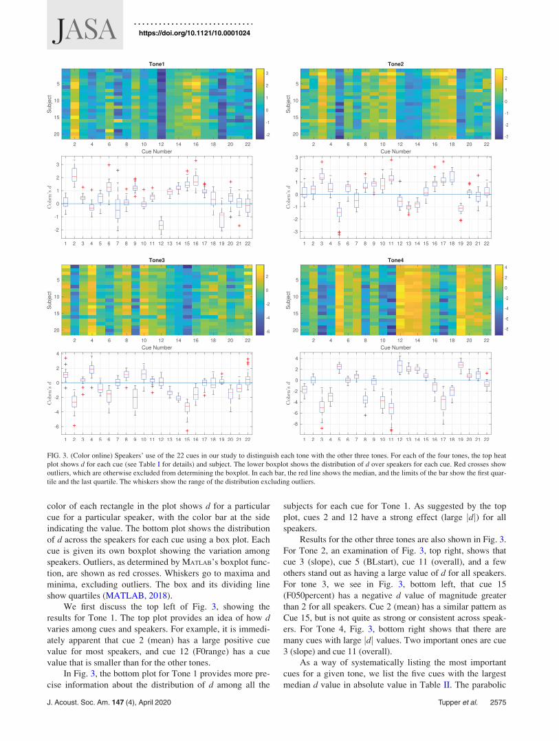
color of each rectangle in the plot shows d for a particular

cue for a particular speaker, with the color bar at the side

indicating the value. The bottom plot shows the distribution

of d across the speakers for each cue using a box plot. Each

cue is given its own boxplot showing the variation among

speakers. Outliers, as determined by MATLAB’s boxplot func-

tion, are shown as red crosses. Whiskers go to maxima and

minima, excluding outliers. The box and its dividing line

show quartiles (MATLAB, 2018).

We first discuss the top left of Fig. 3, showing the

results for Tone 1. The top plot provides an idea of how dvaries among cues and speakers. For example, it is immedi-

ately apparent that cue 2 (mean) has a large positive cue

value for most speakers, and cue 12 (F0range) has a cue

value that is smaller than for the other tones.

In Fig. 3, the bottom plot for Tone 1 provides more pre-

cise information about the distribution of d among all the

subjects for each cue for Tone 1. As suggested by the top

plot, cues 2 and 12 have a strong effect (large jdj) for all

speakers.

Results for the other three tones are also shown in Fig. 3.

For Tone 2, an examination of Fig. 3, top right, shows that

cue 3 (slope), cue 5 (BLstart), cue 11 (overall), and a few

others stand out as having a large value of d for all speakers.

For tone 3, we see in Fig. 3, bottom left, that cue 15

(F050percent) has a negative d value of magnitude greater

than 2 for all speakers. Cue 2 (mean) has a similar pattern as

Cue 15, but is not quite as strong or consistent across speak-

ers. For Tone 4, Fig. 3, bottom right shows that there are

many cues with large jdj values. Two important ones are cue

3 (slope) and cue 11 (overall).

As a way of systematically listing the most important

cues for a given tone, we list the five cues with the largest

median d value in absolute value in Table II. The parabolic

FIG. 3. (Color online) Speakers’ use of the 22 cues in our study to distinguish each tone with the other three tones. For each of the four tones, the top heat

plot shows d for each cue (see Table I for details) and subject. The lower boxplot shows the distribution of d over speakers for each cue. Red crosses show

outliers, which are otherwise excluded from determining the boxplot. In each bar, the red line shows the median, and the limits of the bar show the first quar-

tile and the last quartile. The whiskers show the range of the distribution excluding outliers.


https://doi.org/10.1121/10.0001024

fit cues 2–4 are prominent in the list, as are the raw F0 cues

13–17. The intensity cues 20–22 do not appear, nor does

duration (cue 1).

B. Identifying redundant cues

In reality, the task of identifying a tone does not involve

considering a single cue in isolation. There is no single cue

that is able to distinguish all four tones of Mandarin (unlike,

say, how mean F0 may be able to do so in a language with

level tones such as Yoruba). So it is of interest to identify a

small number of cues that together are able to distinguish all

four tones for all speakers. But we cannot just pick impor-

tant cues independently, because some cues are highly cor-

related. Adding an additional cue can only improve the

ability to distinguish tones if it is to some extent indepen-

dent of the cues already being used. For example, in Table

II both cue 2 (mean) and cue 15 (F050percent) appear twice,

suggesting that they (among other cues) are useful for distin-

guishing tones. But both effectively measure height, so

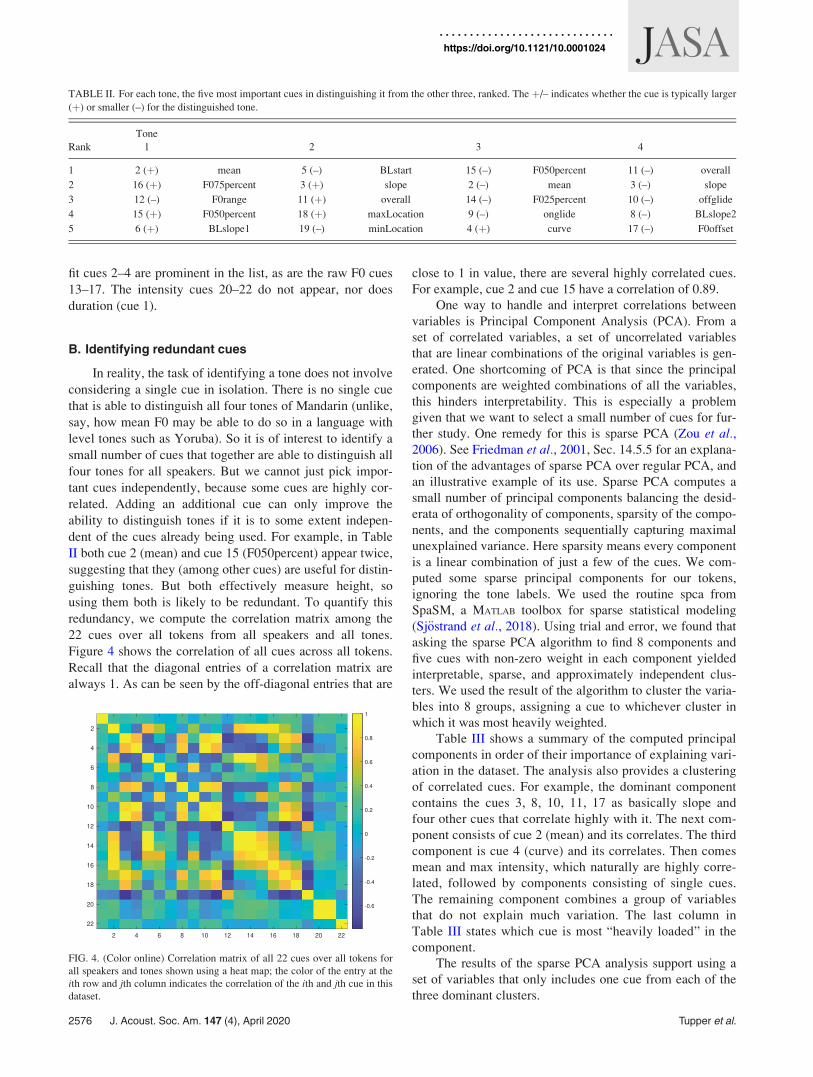
using them both is likely to be redundant. To quantify this

redundancy, we compute the correlation matrix among the

22 cues over all tokens from all speakers and all tones.

Figure 4 shows the correlation of all cues across all tokens.

Recall that the diagonal entries of a correlation matrix are

always 1. As can be seen by the off-diagonal entries that are

close to 1 in value, there are several highly correlated cues.

For example, cue 2 and cue 15 have a correlation of 0.89.

One way to handle and interpret correlations between

variables is Principal Component Analysis (PCA). From a

set of correlated variables, a set of uncorrelated variables

that are linear combinations of the original variables is gen-

erated. One shortcoming of PCA is that since the principal

components are weighted combinations of all the variables,

this hinders interpretability. This is especially a problem

given that we want to select a small number of cues for fur-

ther study. One remedy for this is sparse PCA (Zou et al.,2006). See Friedman et al., 2001, Sec. 14.5.5 for an explana-

tion of the advantages of sparse PCA over regular PCA, and

an illustrative example of its use. Sparse PCA computes a

small number of principal components balancing the desid-

erata of orthogonality of components, sparsity of the compo-

nents, and the components sequentially capturing maximal

unexplained variance. Here sparsity means every component

is a linear combination of just a few of the cues. We com-

puted some sparse principal components for our tokens,

ignoring the tone labels. We used the routine spca from

SpaSM, a MATLAB toolbox for sparse statistical modeling

(Sj€ostrand et al., 2018). Using trial and error, we found that

asking the sparse PCA algorithm to find 8 components and

five cues with non-zero weight in each component yielded

interpretable, sparse, and approximately independent clus-

ters. We used the result of the algorithm to cluster the varia-

bles into 8 groups, assigning a cue to whichever cluster in

which it was most heavily weighted.

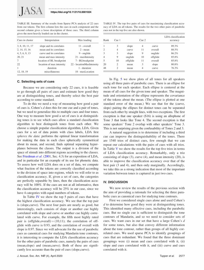
Table III shows a summary of the computed principal

components in order of their importance of explaining vari-

ation in the dataset. The analysis also provides a clustering

of correlated cues. For example, the dominant component

contains the cues 3, 8, 10, 11, 17 as basically slope and

four other cues that correlate highly with it. The next com-

ponent consists of cue 2 (mean) and its correlates. The third

component is cue 4 (curve) and its correlates. Then comes

mean and max intensity, which naturally are highly corre-

lated, followed by components consisting of single cues.

The remaining component combines a group of variables

that do not explain much variation. The last column in

Table III states which cue is most “heavily loaded” in the

component.

The results of the sparse PCA analysis support using a

set of variables that only includes one cue from each of the

three dominant clusters.

TABLE II. For each tone, the five most important cues in distinguishing it from the other three, ranked. The þ/– indicates whether the cue is typically larger

(þ) or smaller (–) for the distinguished tone.

Tone

Rank 1 2 3 4

1 2 (þ) mean 5 (–) BLstart 15 (–) F050percent 11 (–) overall

2 16 (þ) F075percent 3 (þ) slope 2 (–) mean 3 (–) slope

3 12 (–) F0range 11 (þ) overall 14 (–) F025percent 10 (–) offglide

4 15 (þ) F050percent 18 (þ) maxLocation 9 (–) onglide 8 (–) BLslope2

5 6 (þ) BLslope1 19 (–) minLocation 4 (þ) curve 17 (–) F0offset

FIG. 4. (Color online) Correlation matrix of all 22 cues over all tokens for

all speakers and tones shown using a heat map; the color of the entry at the

ith row and jth column indicates the correlation of the ith and jth cue in this

dataset.


https://doi.org/10.1121/10.0001024

C. Selecting sets of cues

Because we are considering only 22 cues, it is feasible

to go through all pairs of cues and estimate how good they

are at distinguishing tones, and thereby select the best pair

according to some standard.

To do this we need a way of measuring how good a pair

of cues is. Cohen’s d does this for one cue and a pair of tones,

but we need to generalize this to multiple cues and four tones.

One way to measure how good a set of cues is at distinguish-

ing tones is to see which cues allow a standard classification

algorithm to best distinguish tones from each other. We

choose a simple popular classification algorithm, LDA. Given

cues for a set of data points with class labels, LDA first

spheres the data: performs the optimal linear transformation

for making the data in each class spherically symmetrical

about its mean, and second, finds optimal separating hyper-

planes between the classes. The output is a division of the

space of stimuli into different regions according to the classes.

See Friedman et al. (2001, Sec. 4.3) for an exposition of LDA,

and in particular for an example of its use for phonetic data.

To assess how well LDA does on a set of data, we compute

what fraction of the tokens are correctly classified according

to the division of space into regions, which we will refer to as

classification accuracy. If, given a set of cues, the categories

are perfectly separable by lines, then the classification accu-

racy will be 100%. If the cues are not at all informative, then

the classification accuracy will be 25% in our case, since we

have 4 categories with equal numbers of tokens.

In Table IV we show the top 5 pairs of cues that have

the highest classification accuracy. We see that the top pair

is (slope,curve). The next four pairs are nearly as good, but

interestingly, each consists of slope or another cue highly

correlated with slope and curve or another cue highly corre-

lated with curve. For example, the fifth most highly rated

pair is (offglide,overall)¼ (10,11); the correlation of off-

glide with curve is 0.93, and the correlation of overall with

slope is 0.97. Since we will advocate for the use of parabolic

cues as canonical cues for studying Mandarin tone contours,

it is interesting to compute the LDA classification accuracy

for the other pairs of parabolic cues, namely the pairs of cues

(mean,slope) and (mean,curve). Both of these are signifi-

cantly less accurate than the pair of cues (slope,curve).

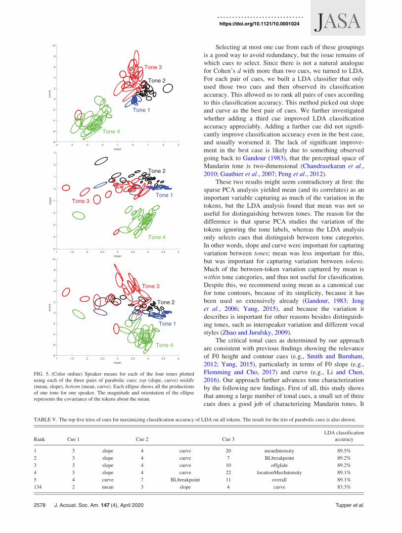
In Fig. 5 we show plots of all tones for all speakers

using all three pairs of parabolic cues. There is an ellipse for

each tone for each speaker. Each ellipse is centered at the

mean of all cues for the given tone and speaker. The magni-

tude and orientation of the ellipse represents the covariance

of the tokens about the mean. (The ellipse is plotted at one

standard error of the mean.) We see that for the (curve,

slope) pairing the ellipses for distinct tones can be separated

from each other by straight lines, with two exceptions. The first

exception is that one speaker (S16) is using an allophone of

Tone 3 that looks like Tone 4. The second exception is that

some speakers’ Tone 2 overlap with other speakers’ Tone 3.

This is not surprising given the confusability of Tones 2 and 3.

A natural suggestion is to determine if including a third

cue can improve the distinguishability of the tones. There

are 1540 trios of distinct cues, few enough that we can

repeat our calculations with the pairs of cues with all trios.

In Table V we show the results for the top five trios in terms

of LDA classification accuracy. Remarkably, only a trio

consisting of slope (3), curve (4), and mean intensity (20), is

able to improve the classification accuracy over that of the

best pair (3 and 4), and then only marginally. Accordingly,

we take this as a strong indication that most of the important

variation between tones is captured in just two cues.

IV. DISCUSSION

We now review the results of the previous section with

the aim of providing a rationale for selecting the three para-

bolic cues as canonical cues for studying tone contours.

First we considered single cues alone and used Cohen’s

d to determine how good they were at distinguishing tones.

This identified many effective cues, including the parabolic

cues. But no single cue is sufficient to distinguish the tone

contours of Mandarin, and so we need to consider sets of

cues. We want cues in our set that have a large Cohen’s dfor some tones, but also that convey different information

about the tone contour, rather than groups of all highly cor-

related cues. We used sparse PCA to identify groupings of

cues that are redundant. We found that the three dominant

groupings were (i) mean and cues correlated with it, (ii)

slope and cues correlated with it, and (iii) curve and cues

correlated with it.

TABLE III. Summary of the results from Sparse PCA analysis of 22 cues

from our tokens. The first column lists the cues in each component and the

second column gives a loose description of those cues. The third column

gives the most heavily loaded cue in the cluster.

Cues in cluster Interpretation Max loading

3, 8, 10, 11, 17 slope and its correlates 11 - overall

2, 14, 15, 16 mean and its correlates 2 - mean

4, 5, 6, 9, 13 curve and its correlates 9 - onglide

20, 21 mean and max intensity 21 - maxIntensity

7 location of BL breakpoint 7 - BLbreakpoint

22 location of max intensity 22 - locationMaxIntensity

1 duration 1 - duration

12, 18, 19 miscellaneous 18 - maxLocation

TABLE IV. The top five pairs of cues for maximizing classification accu-

racy of LDA on all tokens. The results for the two other pairs of parabolic

cues not in the top five are also shown.

LDA classification

Rank Cue 1 Cue 2 accuracy

1 3 slope 4 curve 89.3%

2 4 curve 11 overall 88.5%

3 3 slope 9 onglide 86.2%

4 9 onglide 10 offglide 85.8%

5 10 offglide 11 overall 85.8%

20 2 mean 3 slope 80.8%

48 2 mean 4 curve 76.3%


https://doi.org/10.1121/10.0001024

Selecting at most one cue from each of these groupings

is a good way to avoid redundancy, but the issue remains of

which cues to select. Since there is not a natural analogue

for Cohen’s d with more than two cues, we turned to LDA.

For each pair of cues, we built a LDA classifier that only

used those two cues and then observed its classification

accuracy. This allowed us to rank all pairs of cues according

to this classification accuracy. This method picked out slope

and curve as the best pair of cues. We further investigated

whether adding a third cue improved LDA classification

accuracy appreciably. Adding a further cue did not signifi-

cantly improve classification accuracy even in the best case,

and usually worsened it. The lack of significant improve-

ment in the best case is likely due to something observed

going back to Gandour (1983), that the perceptual space of

Mandarin tone is two-dimensional (Chandrasekaran et al.,2010; Gauthier et al., 2007; Peng et al., 2012).

These two results might seem contradictory at first: the

sparse PCA analysis yielded mean (and its correlates) as an

important variable capturing as much of the variation in the

tokens, but the LDA analysis found that mean was not so

useful for distinguishing between tones. The reason for the

difference is that sparse PCA studies the variation of the

tokens ignoring the tone labels, whereas the LDA analysis

only selects cues that distinguish between tone categories.

In other words, slope and curve were important for capturing

variation between tones; mean was less important for this,

but was important for capturing variation between tokens.

Much of the between-token variation captured by mean is

within tone categories, and thus not useful for classification.

Despite this, we recommend using mean as a canonical cue

for tone contours, because of its simplicity, because it has

been used so extensively already (Gandour, 1983; Jeng

et al., 2006; Yang, 2015), and because the variation it

describes is important for other reasons besides distinguish-

ing tones, such as interspeaker variation and different vocal

styles (Zhao and Jurafsky, 2009).

The critical tonal cues as determined by our approach

are consistent with previous findings showing the relevance

of F0 height and contour cues (e.g., Smith and Burnham,

2012; Yang, 2015), particularly in terms of F0 slope (e.g.,

Flemming and Cho, 2017) and curve (e.g., Li and Chen,

2016). Our approach further advances tone characterization

by the following new findings. First of all, this study shows

that among a large number of tonal cues, a small set of three

cues does a good job of characterizing Mandarin tones. It

TABLE V. The top five trios of cues for maximizing classification accuracy of LDA on all tokens. The result for the trio of parabolic cues is also shown.

LDA classification

Rank Cue 1 Cue 2 Cue 3 accuracy

1 3 slope 4 curve 20 meanIntensity 89.5%

2 3 slope 4 curve 7 BLbreakpoint 89.2%

3 3 slope 4 curve 10 offglide 89.2%

4 3 slope 4 curve 22 locationMaxIntensity 89.1%

5 4 curve 7 BLbreakpoint 11 overall 89.1%

134 2 mean 3 slope 4 curve 83.3%

FIG. 5. (Color online) Speaker means for each of the four tones plotted

using each of the three pairs of parabolic cues: top (slope, curve) middle(mean, slope), bottom (mean, curve). Each ellipse shows all the productions

of one tone for one speaker. The magnitude and orientation of the ellipse

represents the covariance of the tokens about the mean.


https://doi.org/10.1121/10.0001024

further reveals that cues can be clustered into groups such

that those within each group are functionally equivalent,

resulting in multiple possible choices of 3-cue sets that can

effectively distinguish different tones. Moreover, our analy-

sis brings the parabolic cues to the forefront. The three cues

obtained from the parabolic fit (F0 mean, slope, and curve)

are considered the optimal cue set since they are easy to

compute, directly interpretable, and among the best for

distinguishing tones.

On the practical front, there are additional reasons

besides our statistical analyses to favor using the three para-

bolic cues as a standard for studying tone contours. First,

there is value in having a small critical set of standard cues

whatever they may be. If different groups use different cues

then it is difficult or impossible to compare results from dif-

ferent papers. For example, if an experimental manipulation

is found to lead to a shift in turning point of Tone 2 in one

study and an increase in curve in another, it is possible that

they are observing the same phenomenon, but it is difficult

to know for sure without reperforming the analysis with the

raw data. Another reason to use only a small number of cues

is to reduce the temptation to select the cues for any dataset

that give the most significant results, thus leading to false

positive results.

Finally, fitting a parabola to a curve is very well under-

stood mathematically and statistically (unlike the nonlinear

regression required for the broken line fit). There are effi-

cient algorithms for computing them available in every

mathematical software system. The fact that our three cues

are based on basic mathematics (the Legendre polynomials

being standard tools used in many contexts) and not any spe-

cific facts about Mandarin tone contours means that they

can be generalized to other languages and tone systems.

Our results also have implications for the relationship

between tone perception and production. Lexical tone

perceptual studies have been largely influenced by Gandour

(1983), which determined that tone perception involves

“height” and “direction” as the two perceptual dimensions

that have been interpreted as F0 mean and slope, respectively

(e.g., Chandrasekaran et al., 2010; Francis et al., 2008;

Guion and Pederson, 2007; Jongman et al., 2017). Moreover,

native Mandarin listeners give stronger perceptual weight-

ings to “direction” than to “height” (Francis et al., 2008;

Gandour, 1983). Our study corroborates these findings in

that slope was important for capturing between-categoryclassifications of our participants’ tone productions, whereas

mean was important for explaining between-token variations

that are within categories. These suggest that the differential

cue weighting pattern may reflect the between-category func-

tion for direction and between-token function for height in

perception. In addition to mean and slope, our study has

demonstrated that curve is an important cue for between-

category classification. However, curve as a tone perceptual

cue has not been widely explored. Perceptual cues that are

related to curve include TP and DF0, since any change in

these cues should lead to a change in the parabolic shape of

the tone contour and have been shown to influence the

perception of Tone 2 and Tone 3 (Moore and Jongman,

1997). A recent study by Leung and Wang (2018) also shows

that curve demonstrates a stronger correlation between the

production and perception of Tone 2 than slope. However,

further research is needed to examine the role of curve in the

perception-production link of all Mandarin tones, as well as

other tone languages.

The current results also have implications for establish-

ing the relationship between tone acoustics and articulation.

Research has revealed that, during tone production, facial

(e.g., head, eyebrow, lip) movements in distance, direction,

speed, and timing can be spatially and temporally equated to

acoustic features of tonal changes in F0 (Attina et al., 2010;

Garg et al., 2019). For example, Garg et al. (2019) shows

that the upward and downward head and eyebrow move-

ments follow the rising, dipping, and falling tone trajectories

for Mandarin contour tones (i.e., Tone 2, Tone 3, and Tone

4, respectively). Additionally, the time taken for the move-

ments to reach the maximum displacement is also aligned

with these trajectories. These results suggest that the spatial

and temporal dynamics in the articulation of different tones

may particularly be aligned with the parabolic cues identi-

fied by the current study as the critical cues in representing

tonal contours, reflecting a linguistically meaningful associ-

ation between spatial and acoustic events in lexical tone

production. Further research may thus explore how these

cross-modal (articulatory-acoustic) resources can be incor-

porated in tone perception.

ACKNOWLEDGMENTS

This project has been supported by research grants from

the Natural Sciences and Engineering Research Council of

Canada (NSERC Discovery Grant No. 2017-05978) and the

Social Sciences and Humanities Research Council of

Canada (SSHRC Insight Grant No. 435-2012-1641). We

thank SFU Language and Brain Lab members Zoe Beukers,

Anisa Dhanji, Hasti Halakoeei, Abner Hernandez, Michelle

Le, Kelsey Philip, Michelle Ramsay, and Joanna Xie for

conducting acoustic data measurements. Portions of this

research were presented at the 176th Meeting of the

Acoustical Society of America and 2018 Acoustics Week in

Canada, Victoria, British Columbia, Canada.

Attina, V., Gibert, G., Vatikiotis-Bateson, E., and Burnham, D. (2010).

“Production of Mandarin lexical tones: Auditory and visual components,”

in Auditory-Visual Speech Processing 2010.

Barry, J. G., and Blamey, P. J. (2004). “The acoustic analysis of tone differ-

entiation as a means for assessing tone production in speakers of

Cantonese,” J. Acoust. Soc. Am. 116(3), 1739–1748.

Black, A. W., and Hunt, A. J. (1996). “Generating F0 contours from ToBI

labels using linear regression,” in Proceedings of the Fourth InternationalConference on Spoken Language Processing ICSLP 1996, IEEE, Vol. 3,

pp. 1385–1388.

Blicher, D. L., Diehl, R. L., and Cohen, L. B. (1990). “Effects of syllable

duration on the perception of the Mandarin Tone 2/Tone 3 distinction:

Evidence of auditory enhancement,” J. Phonetics 18(1), 37–49.

Boersma, P., and Weenink, D. (2017). “Praat, a system for doing phonetics

by computer (version 6.0. 28),” Institute of Phonetic Sciences University

of Amsterdam (up-to-date version of the manual available at http://

www.fon.hum.uva.nl/praat/).


https://doi.org/10.1121/10.0001024

Carroll, J. D., and Chang, J.-J. (1970). “Analysis of individual differences

in multidimensional scaling via an n-way generalization of ‘Eckart-

Young’ decomposition,” Psychometrika 35(3), 283–319.

Chandrasekaran, B., Sampath, P. D., and Wong, P. C. (2010). “Individual

variability in cue-weighting and lexical tone learning,” J. Acoust. Soc.

Am. 128(1), 456–465.

Chen, S., Zhang, C., McCollum, A. G., and Wayland, R. (2017). “Statistical

modelling of phonetic and phonologised perturbation effects in tonal and

non-tonal languages,” Speech Commun. 88, 17–38.

Chuang, C., Hiki, S., Sone, T., and Nimura, T. (1972). “The acoustical fea-

tures and perceptual cues of the four tones of standard colloquial

Chinese,” in Proceedings of the Seventh International Congress onAcoustics (Akademiai Kiado, Budapest), pp. 297–300.

Cohen, J. (1988). Statistical Power Analysis for the Social Sciences(Erlbaum, Hillsdale, New Jersey).

Flemming, E., and Cho, H. (2017). “The phonetic specification of contour

tones: Evidence from the Mandarin rising tone,” Phonology 34(1), 1–40.

Francis, A. L., Ciocca, V., Ma, L., and Fenn, K. (2008). “Perceptual learn-

ing of Cantonese lexical tones by tone and non-tone language speakers,”

J. Phonetics 36(2), 268–294.

Friedman, J., Hastie, T., and Tibshirani, R. (2001). The Elements ofStatistical Learning, Vol. 1 (Springer, New York).

Fu, Q.-J., and Zeng, F.-G. (2000). “Identification of temporal envelope cues

in Chinese tone recognition,” Asia Pacific J. Speech Lang. Hear. 5(1),

45–57.

Fu, Q.-J., Zeng, F.-G., Shannon, R. V., and Soli, S. D. (1998). “Importance

of tonal envelope cues in Chinese speech recognition,” J. Acoust. Soc.

Am. 104(1), 505–510.

Gandour, J. (1983). “Tone perception in Far Eastern languages,”

J. Phonetics 11(2), 149–175.

Garg, S., Hamarneh, G., Jongman, A., Sereno, J. A., and Wang, Y. (2019).

“Computer-vision analysis reveals facial movements made during

Mandarin tone production align with pitch trajectories,” Speech

Commun. 113, 47–62.

Gauthier, B., Shi, R., and Xu, Y. (2007). “Learning phonetic categories by

tracking movements,” Cognition 103(1), 80–106.

Ghosh, P. K., and Narayanan, S. S. (2009). “Pitch contour stylization using

an optimal piecewise polynomial approximation,” IEEE Signal Proc. Let.

16(9), 810–813.

Guion, S. G., and Pederson, E. (2007). “Investigating the role of attention in

phonetic learning,” in Language Experience in Second Language SpeechLearning (John Benjamins Publishing Co., Amsterdam), pp. 57–77.

Hirst, D., and Espesser, R. (1993). “Automatic modelling of fundamental

frequency using a quadratic spline function,” Travaux de l’Institut de

phon�etique d’Aix 15, 71–85.

Howie, J. M., and Howie, J. M. (1976). Acoustical Studies of MandarinVowels and Tones, Vol. 18 (Cambridge University Press, Cambridge).

Jeng, J.-Y., Weismer, G., and Kent, R. D. (2006). “Production and percep-

tion of Mandarin tone in adults with cerebral palsy,” Clin. Linguist.

Phonet. 20(1), 67–87.

Jongman, A., Qin, Z., Zhang, J., and Sereno, J. A. (2017). “Just noticeable

differences for pitch direction, height, and slope for Mandarin and

English listeners,” J. Acoust. Soc. Am. 142(2), EL163–EL169.

Khouw, E., and Ciocca, V. (2007). “Perceptual correlates of Cantonese

tones,” J. Phonetics 35(1), 104–117.

Komzsik, L. (2017). Approximation Techniques for Engineers (CRC Press,

Boca Raton, Florida).

Kong, Y.-Y., and Zeng, F.-G. (2006). “Temporal and spectral cues in

Mandarin tone recognition,” J. Acoust. Soc. Am. 120(5), 2830–2840.

Lehiste, I. (1970). Suprasegmentals (MIT Press, Cambridge, Massachusetts).

Leung, K. K., and Wang, Y. (2018). “The relation between production and

perception of Mandarin tone,” J. Acoust. Soc. Am. 144(3), 1721–1721.

Li, Q., and Chen, Y. (2016). “An acoustic study of contextual tonal varia-

tion in Tianjin Mandarin,” J. Phonetics 54, 123–150.

Liu, S., and Samuel, A. G. (2004). “Perception of Mandarin lexical tones

when F0 information is neutralized,” Lang. Speech 47(2), 109–138.

MATLAB (2018). Version 7.10.0 (R2018b) (The MathWorks Inc., Natick,

Massachusetts).

Moore, C. B., and Jongman, A. (1997). “Speaker normalization in the per-

ception of Mandarin Chinese tones,” J. Acoust. Soc. Am. 102(3),

1864–1877.

Patten, M. L., and Newhart, M. (2017). Understanding Research Methods:An Overview of the Essentials (Routledge, Abingdon-on-Thames).

Peng, G., Zhang, C., Zheng, H.-Y., Minett, J. W., and Wang, W. S.-Y.

(2012). “The effect of intertalker variations on acoustic–perceptual map-

ping in Cantonese and Mandarin tone systems,” J. Speech Lang. Hear. R.

55(2), 579–595.

Prom-On, S., Liu, F., and Xu, Y. (2012). “Post-low bouncing in Mandarin

Chinese: Acoustic analysis and computational modeling,” J. Acoust. Soc.

Am. 132(1), 421–432.

Prom-On, S., Xu, Y., and Thipakorn, B. (2009). “Modeling tone and intona-

tion in Mandarin and English as a process of target approximation,”

J. Acoust. Soc. Am. 125(1), 405–424.

Rivlin, T. J. (1981). An Introduction to the Approximation of Functions(Courier Corporation, North Chelmsford, Massachusetts).

Rosen, S. (1992). “Temporal information in speech: Acoustic, auditory and

linguistic aspects,” Philos. T. R. Soc. B 336, 367–373.

Shih, C., and Lu, H.-Y. D. (2015). “Effects of talker-to-listener distance on

tone,” J. Phonetics 51, 6–35.

Sj€ostrand, K., Clemmensen, L. H., Larsen, R., Einarsson, G., and Ersbøll,

B. K. (2018). “SpaSM: A MATLAB toolbox for sparse statistical modeling,”

J. Stat. Softw. 84(10), 1–37.

Smith, D., and Burnham, D. (2012). “Facilitation of Mandarin tone percep-

tion by visual speech in clear and degraded audio: Implications for

cochlear implants,” J. Acoust. Soc. Am. 131(2), 1480–1489.

Wang, S., Xu, L., and Mannell, R. (2011). “Relative contributions of tem-

poral envelope and fine structure cues to lexical tone recognition in

hearing-impaired listeners,” JARO 12, 783–794.

Wang, Y., Jongman, A., and Sereno, J. A. (2003). “Acoustic and perceptual

evaluation of Mandarin tone productions before and after perceptual train-

ing,” J. Acoust. Soc. Am. 113(2), 1033–1043.

Whalen, D. H., and Xu, Y. (1992). “Information for Mandarin tones in the

amplitude contour and in brief segments,” Phonetica 49(1), 25–47.

Wong, P., Fu, W. M., and Cheung, E. Y. (2017). “Cantonese-speaking children

do not acquire tone perception before tone production: A perceptual and acous-

tic study of three-year-olds’ monosyllabic tones,” Front. Psychol. 8, 1450.

Xu, Y. (2001). “Fundamental frequency peak delay in Mandarin,”

Phonetica 58(1–2), 26–52.

Xu, Y. (2005). “Speech melody as articulatorily implemented communica-

tive functions,” Speech Commun. 46(3–4), 220–251.

Xu, Y., and Wang, Q. E. (2001). “Pitch targets and their realization:

Evidence from Mandarin Chinese,” Speech Commun. 33(4), 319–337.

Yang, B. (2015). Perception and Production of Mandarin Tones by NativeSpeakers and L2 Learners (Springer, New York).

Zhang, J., and Meng, Y. (2016). “Structure-dependent tone Sandhi in real

and Nonce disyllables in Shanghai Wu,” J. Phonetics 54, 169–201.

Zhao, T. C., and Kuhl, P. K. (2015). “Effect of musical experience on

learning lexical tone categories,” J. Acoust. Soc. Am. 137(3),

1452–1463.

Zhao, Y., and Jurafsky, D. (2009). “The effect of lexical frequency and

Lombard reflex on tone hyperarticulation,” J. Phonetics 37(2),

231–247.

Zou, H., Hastie, T., and Tibshirani, R. (2006). “Sparse principal component

analysis,” J. Comput. Graph. Stat. 15(2), 265–286.


https://doi.org/10.1121/10.0001024

Documents

Characterizing the distinctive acoustic cues of Mandarin tones