Characterizing Learning by Simultaneous Analysis of

Innovative Methodology

Characterizing Learning by Simultaneous Analysis of Continuous and BinaryMeasures of Performance

M. J. Prerau,1,7 A. C. Smith,1 Uri T. Eden,6,7 Y. Kubota,2,3 M. Yanike,4 W. Suzuki,4

A. M. Graybiel,2,3 and E. N. Brown1,2,5

1Department of Anesthesia and Critical Care, Massachusetts General Hospital, Boston, Massachusetts; 2Department of Brain andCognitive Sciences and 3McGovern Institute for Brain Research, Massachusetts Institute of Technology, Cambridge, Massachusetts;4Center for Neural Science, New York University, New York City, New York; 5Division of Health Sciences and Technology, HarvardMedical School/Massachusetts Institute of Technology, Cambridge, Massachusetts; 6Department of Mathematics and Statistics and7Program in Neuroscience, Boston University, Boston, Massachusetts

Submitted 24 November 2008; accepted in final form 17 August 2009

Prerau MJ, Smith AC, Eden UT, Kubota Y, Yanike M, Suzuki W,Graybiel AM, Brown EN. Characterizing learning by simultaneousanalysis of continuous and binary measures of performance. J Neu-rophysiol 102: 3060–3072, 2009. First published August 19, 2009;doi:10.1152/jn.91251.2008. Continuous observations, such as reac-tion and run times, and binary observations, such as correct/incorrectresponses, are recorded routinely in behavioral learning experiments.Although both types of performance measures are often recordedsimultaneously, the two have not been used in combination to evaluatelearning. We present a state-space model of learning in which theobservation process has simultaneously recorded continuous and bi-nary measures of performance. We use these performance measuressimultaneously to estimate the model parameters and the unobservedcognitive state process by maximum likelihood using an approximateexpectation maximization (EM) algorithm. We introduce the conceptof a reaction-time curve and reformulate our previous definitions ofthe learning curve, the ideal observer curve, the learning trial andbetween-trial comparisons of performance in terms of the new model.We illustrate the properties of the new model in an analysis of asimulated learning experiment. In the simulated data analysis, simul-taneous use of the two measures of performance provided morecredible and accurate estimates of the learning than either measureanalyzed separately. We also analyze two actual learning experimentsin which the performance of rats and of monkeys was tracked acrosstrials by simultaneously recorded reaction and run times and thecorrect and incorrect responses. In the analysis of the actual experi-ments, our algorithm gave a straightforward, efficient way to charac-terize learning by combining continuous and binary measures ofperformance. This analysis paradigm has implications for character-izing learning and for the more general problem of combining differ-ent data types to characterize the properties of a neural system.

I N T R O D U C T I O N

Learning is a dynamic process that can be defined as achange in behavior that occurs as a result of experience.Learning is often studied by demonstrating that after a series oftrials, a subject can perform a previously unfamiliar task morereliably than what would be predicted by chance. The ability ofa subject to learn a new task is commonly tested to study theeffect of learning on genetic manipulations (Rondi-Reig et al.2001) brain lesions (Dias et al. 1997; Dusek and Eichenbaum

1997; Fox et al. 2003; Roman et al. 1993; Whishaw and Tomie1991; Wise and Murray 1999), pharmacological interventions(Stefani et al. 2003), and electrical stimulation (Williams andEskandar 2006). Accurate characterizations of learning are alsoneeded to link behavioral changes to changes in neural activityin target brain regions (Barnes et al. 2005; Jog et al. 1999; Lawet al. 2005; Wirth et al. 2003).

Binary measurements, such as the sequence of correct andincorrect responses, are the measurements most typically re-corded to track behavioral changes in learning experiments.Performance is characterized by estimating a learning curvethat defines the probability of a correct response as a functionof trial number and/or by identifying the learning trial, i.e., thetrial on which the change in behavior suggestive of learningcan be established using a statistical criterion (Gallistel et al.2004; Jog et al. 1999; Siegel and Castellan 1988; Smith et al.2004, 2005; Wirth et al. 2003).

Continuous measurements such as the reaction time (thetime it takes the subject to react to a stimulus), the responsetime, and the total amount of time it takes the subject toexecute a task or the task velocity, are also frequently recordedin learning experiments. A separate analysis of the continuousmeasurements is often presented to support the findings of, orapparent behavior identified in, the analysis of the binaryobservations.

A frequent assumption in learning studies is that with re-peated exposure to the task the subject will show an improve-ment in performance (Usher and McClelland 2001). Thisphenomenon is frequently represented by assuming a mono-tonic relation between exposure to the task (trial number) andthe measure of performance (Gallistel et al. 2004). As aconsequence, deterministic logistic or sigmoid functions areoften fit to each type of performance measure separately.

In no case have the continuous and the binary measurementsbeen analyzed together to characterize learning. Combinedanalysis of continuous and binary data may be a valuable wayto study formally whether it is plausible to assume a commonmechanism underlying both measures of performance. Whenplausible, a combined analysis may improve the statisticalpower of the study. In addition, for cases in which a subject hasreached a plateau in his/her binary responses, i.e., gives allcorrect responses, yet continues to perform the task withincreasingly faster reaction times, examining only the binaryresponses would suggest that learning has ceased, whereas the

Address for reprint requests and other correspondence: E. N. Brown,Neuroscience Statistics Research Laboratory, Dept. of Anesthesia and CriticalCare, Massachusetts General Hospital, 55 Fruit St, Clinics 3, Boston, MA02114-2696 (E-mail: [email protected]).

J Neurophysiol 102: 3060–3072, 2009.First published August 19, 2009; doi:10.1152/jn.91251.2008.

3060 0022-3077/09 $8.00 Copyright © 2009 The American Physiological Society www.jn.org

Downloaded from journals.physiology.org/journal/jn (024.002.156.129) on January 15, 2021.

faster reaction times would suggest that the subject is continu-ing to refine his/her understanding of the task.

We recently introduced a state-space approach to character-izing learning in behavioral experiments (Smith et al. 2004,2005, 2007; Wirth et al. 2003). To develop a dynamic approachto analyzing data from learning experiments in which contin-uous and binary responses are simultaneously recorded, weextend our previously developed state-space model of learningto include both a lognormal probability model for the contin-uous measurements and a Bernoulli probability model for thebinary measurements. We estimate the model using an approx-imate EM algorithm (Dempster et al. 1977) to compute thereaction-time curve, the learning curve, the ideal observercurve, the learning trial, and between-trial comparisons ofperformance. We illustrate our approach in the analysis of asimulated learning experiment and two actual learning exper-iments: one in which a monkey rapidly learns new associationswithin a single session and another in which a mouse slowlylearns a T-maze task over many days.

M E T H O D S

State-space model of learning

We assume that learning is a dynamic process that can be studiedwith the state-space framework used in engineering, statistics andcomputer science (Doucet et al. 2001; Durbin and Koopman 2001;Fahrmeir and Tutz 2001; Kitagawa and Gersch 1996; Mendel 1995;Smith and Brown 2003). The state-space model consists of twoequations: a state equation and an observation equation. The stateequation defines the temporal evolution of an unobservable process.Such state models with unobservable processes are often referred to ashidden Markov or latent process models (Fahrmeir and Tutz 2001;Smith and Brown 2003; Smith et al. 2004, 2005). In our analysis, thestate equation defines an unobservable cognitive state that representsthe subject’s understanding of the task. The evolution of this cognitivestate is tracked across the trials in the experiment. We formulate themodel so that the state increases as learning occurs and decreaseswhen learning does not occur. The observation equation defines howthe observed data relate to the cognitive state process. The data weobserve in the learning experiment are the series of continuous andbinary responses. The objective of the analysis is to characterizelearning by estimating the cognitive state process using simulta-neously both sets of data.

We consider a learning experiment consisting of k trials in which oneach trial a continuous and a binary response measurement of perfor-mance are recorded. Let rk and nk be, respectively, the values of thecontinuous and binary measurements on trial k for k � 1, . . . , K. Weassume that the cognitive state model is the first-order autoregressive[AR(1)] process

xk � �xk�1 � �k (1)

where 0 � � � 1 represents a forgetting factor, the vk are independent,zero mean Gaussian random variables with variance �v

2 . Let x � [x0,x1, . . . , xK] be the unobserved cognitive state process for the entireexperiment.

For the purpose of exposition, we assume that the continuousmeasurements are reaction times and that the observation model forthe reaction times is

zk � log rk � � � �xk � �k (2)

where the �k are independent zero mean Gaussian random variableswith variance ��

2. Formulation of the log of the reaction time rk as alinear function of the cognitive state variable ensures that at each trial

the reaction time is positive. We assume that � � 0 to ensure that onaverage, as the cognitive state xk increases with learning, the reactiontime decreases. We let Z � [z1, . . . , zK] be the log of the reactiontimes on all trials.

We assume that the observation model for the binary responses isthe Bernoulli probability model

Pr�nk � xk� � pknk �1 pk�

1�nk (3)

where pk, the probability of a correct response on trial k, is defined interms of the unobserved cognitive state process as

pk � exp�� xk��1 � exp�� xk��1 (4)

Formulation of pk as a logistic function of the cognitive state process(Eq. 4) ensures that the probability of a correct response on each trialis constrained to lie between 0 and 1 and that as the cognitive stateincreases, the probability of a correct responses approaches 1. Weestimate the parameter � from pchance, the probability of a correctresponse by chance at the outset of the experiment. To do so, weassume that there is no bias in the subject’s responses at the outset ofthe experiment, and we set p0 the probability of a correct response atthe outset of the experiment equal to pchance For example, if thesubject is executing a binary choice task, then the probability of acorrect response by chance is pchance � 0.5. Therefore using Eq. 4,with k � 0, p0 � pchance, and x0 � 0, we solve for the estimate of �as �̂ � log[(1 � pchance)

�1pchance]. After estimating the cognitivestate process and the model parameters from the data across the entirelearning experiment (described in the following text), the estimate ofx0, x̂0, may take on a value other than 0. If this is the case, then fromEq. 4, the final estimate of the probability of a correct response at theoutset of the experiment, p̂0 � [1 � exp(�̂ � x̂0)]�1 exp(�̂ � x̂0), willdiffer from pchance. Any difference between p̂0 and pchance is due to x̂0

not equaling 0 and suggests a potential learning bias for the subject.We let N � [n1, . . . , nK] be the sequence of correct and incorrectresponses on all trials.

The state model (Eq. 1) provides a stochastic continuity constraint(Kitagawa and Gersch 1996) so that the current cognitive state, thereaction time (Eq. 2), and the probability of a correct response (Eq. 4)depend on the prior cognitive state. In this way, the state-space modelprovides a simple, plausible framework for relating performance onsuccessive trials of the experiment.

Because x is unobservable and because � � (�, �, �, �v2, ��

2, x0) isa set of unknown parameters, we use the expectation-maximization(EM) algorithm to estimate them by maximum likelihood (Dempsteret al. 1977). The EM algorithm is a well-known procedure forperforming maximum likelihood estimation when there is an unob-servable process or missing observations. The EM algorithm has beenused to estimate state-space models from point process and binaryobservations with linear Gaussian state processes (Smith and Brown2003; Smith et al. 2004, 2005). The current EM algorithm combinesfeatures of the ones in Shumway and Stoffer (1982) and Smith andBrown (2003). The key technical point that allows implementation ofthis algorithm is the combined filter algorithm in Eqs. A4–A8 ofAPPENDIX A. Its derivation is given in Prerau et al. (2008).

Estimation of the reaction-time and learning curves

Because we compute the maximum likelihood estimate of � � (�,�, �, �v

2, ��2, x0) using the EM algorithm, we compute the maximum

likelihood estimate of each xk for k � 1, . . . , K from the fixed-intervalsmoothing algorithm at the last iteration of the EM algorithm (Eqs.A9–A11). That is, the smoothing algorithm estimate at trial k is theestimate of xk given Z and N with � replaced by its maximumlikelihood estimate. Hence because the smoothing algorithm is basedon all the data, it gives the estimate of the cognitive state from theperspective of the ideal observer. This estimate is both the maximumlikelihood and empirical Bayes’ estimate of xk (Fahrmeir and Tutz


3061COGNITIVE STATE ESTIMATION

J Neurophysiol • VOL 102 • NOVEMBER 2009 • www.jn.org


2001). The smoothing algorithm estimates the state as the Gaussianrandom variable with mean xk�K (Eq. A9) and variance, �k�K

2 (Eq. A11),where the notation xk�K denotes the estimate of the cognitive stateprocess at trial k given all of the data in the experiment. The stateestimates have Gaussian distributions because we use Gaussian ap-proximations to compute them in the filter (Eqs. A4–A8) and smooth-ing algorithms (Eqs. A9–A11).

Using the smoothing algorithm estimate of xk, we can compute theprobability density of the estimate of the log reaction time at trial k,rk, by using Eq. 2 and the standard change-of-variables formula fromelementary probability theory (Rice 2007; Smith et al. 2004). Apply-ing the change-of-variable formula to the relation rk � exp(� � �xk)and the fact that, conditional on the data Z and N, xk has anapproximate Gaussian probability density with mean xk�K (Eq. A9) andvariance �k�K

2 (Eq. A11), yields as the probability density of rk giventhe data Z and N

f�r � �, xk�K, � k�K2 �

�1

r��2 � k�K

2 ��12 exp� 1

2� k�K2 �log �r ��

� xk�K�2� (5)

Eq. 5 is the probability density of a log normal random variable (Rice2007). We define the reaction-time curve as the plot of rk�K versus kfor k � 1, . . . , K, where rk�K is the mode of Eq. 5.

Similarly, if we apply the change-of-variables formula to therelation pk � exp(� � xk)[1 � exp(� � xk)]

�1 and use again the factthat conditional on the data, Z and N, xk has an approximate Gaussianprobability density with mean xk�K and variance �k�K

2 , we obtain theprobability density of pk given the data Z and N

f�p � �, xk�K, � k�K2 �

�1

p�1 p��2 � k�K

2 ��12 exp� 1

2� k�K2 �log� p

�1 p�exp�� xk�K�2�

(6)

We define the learning curve as the plot of pk�K versus k for k �1, . . . , K, where pk�K is the mode of Eq. 6. The derivations of Eqs. 5and 6 are given in APPENDIX B.

Ideal observer curve

To characterize learning, we need a systematic way to compareperformance on each trial with performance on any other trial. Ofparticular importance is comparing performance on each trial withperformance at the start of the experiment. If performance becomesconsistently better than performance at the outset of the experimentand remains so for the balance of the experiment, it is plausible toconclude that learning has occurred. If in the learning experiment weonly observed the subject’s reaction times on each trial, then we canuse the probability density for the learning curve in Eq. 5 to computethe ideal observer curve as

Pr�rk�K � r0� (7)

for k � 1, . . . , K. The reaction-time ideal observer curve computes ateach trial k the probability that the reaction time at trial k is less thanthe reaction time at the outset of the experiment. Similarly, if only thebinary responses are observed, then we use Eq. 6 to compute the idealobserver curve as

Pr�pk�K � p0� (8)

for k � 1, . . . , K. The binary response ideal observer curve describesfor each trial k the probability that pk is greater than the probability ofa correct response at the outset of the experiment.

To generalize these definitions so that we can use simultaneouslythe reaction-time and binary behavioral observations, we note thatfor both the reaction-time and binary observations, the idealobserver curve can be expressed in terms of the cognitive statevariables as

Pr�xk�K � x0� � Pr�rk�K � r0� � Pr�pk�K � p0� (9)

because rk�K and pk�K are monotonic functions of xk�K. Therefore if thereaction-time and binary observations are both used to estimate thecognitive state process, then the ideal observer curve for the jointobservations is defined by the left side of Eq. 9. Moreover, if onlyreaction times or the binary responses are observed, then Eq. 9 agreeswith the individual ideal observer curves for these measurements.Therefore we define Eq. 9 as the ideal observer curve for thecombined model.

Identification of the learning trial

Although learning is a dynamic process, it is helpful to have asingle summary that indicates where in the experiment performance isbetter than at the outset. We identify the learning trial from the idealobserver curve. We define the learning trial as the first trial for whichthe ideal observer can state with reasonable certainty that the subjectperforms better on that trial and all subsequent trials than at the outsetof the experiment. For our analyses we define a level of reasonablecertainty as 0.975 and term this trial the ideal observer learning trialwith level of certainty 0.975 [IO (0.975)]. The IO(0.975) is the firsttrial j such that for all trials k � j

Pr�xk � x0� � 0.975 (10)

Between-trial comparisons of performance

We make between-trial comparisons of learning that are not re-stricted to comparisons between a given trial and performance at theoutset of the experiment. These comparisons can be performed in astraightforward way in our paradigm because we estimate the jointprobability distribution of x from the smoothing algorithm at the finaliteration of the EM algorithm (Eqs. A9–A11). Therefore given anytwo trials, we can compute the probability that the subject’s perfor-mance on one trial is better than the performance on the other trial.The transformation between the state variable and the probability of acorrect response and the transformation between the state variableand the reaction time are monotonic. Therefore it suffices tocompute the probability that the cognitive state at trial k is greaterthan the cognitive state on trial j for all distinct pairs k and j. Tocompute the probability Pr(xk xj) for all pairs j � 1, . . . , K � 1and k � 2, . . . , K, we use a Monte Carlo algorithm, whichcombines the fixed-interval smoothing and the state-space covari-ance algorithm at the last step of the EM algorithm to compute thecovariance between the states at two different trials (Smith et al.2004, 2005). This algorithm compares pairs of random variablesfrom the K-dimensional joint probability density of the cognitivestate process.

Experimental protocols for learning

CONDITIONAL T-MAZE TASK. To illustrate our method applied toan actual learning experiment, we analyzed the responses of amouse performing a T-maze task, similar to those described in Joget al. (1999) and in Barnes et al. (2005). In this task, the mouse wasrequired to use tactile cues (rough or smooth surface of the mazefloor) to learn which one of two arms of a T-maze to enter toreceive a reward. On each day of this 13-day experiment, themouse performed 28 – 40 trials. The total number of trials was 461.In each trial, the mouse had to acquire the cue-turn association to


3062 PRERAU, SMITH, EDEN, KUBOTA, YANIKE, SUZUKI, GRAYBIEL, AND BROWN



succeed. For this experiment, the probability of making a correctresponse by chance was 0.5. To characterize learning, we recordedat each trial the run time (the time from the animal’s onset oflocomotion to its arrival at the goal), and whether the animal’schoice of goal arm was correct or incorrect. The objective of thisstudy was to relate changes in learning across days to concurrentchanges in neural activity in the striatum (Barnes et al. 2005; Joget al. 1999).

LOCATION-SCENE ASSOCIATION TASK. As a second illustration ofour methods applied to an actual learning experiment, we analyzed theresponses of a macaque monkey in a location-scene association task,described in detail in Wirth et al. (2003). In this task, each trial startedwhen the monkey fixated on a centrally presented cue on a computerscreen. The animal was then presented with four identical targets(north, south, east, and west) superimposed on a novel visual scene.After the scene disappeared, the targets remained on the screen duringa delay period. At the end of the delay period, the fixation pointdisappeared cueing the animal to make an eye-movement to one of thethree targets. For each scene, only one target was rewarded and thepositions of rewarded locations were counterbalanced across all newscenes. Between two to three novel scenes were typically learnedsimultaneously and trials of novel scenes were interspersed with trialsin which three well-learned scenes were presented. Because therewere three locations the monkey could choose as a response, theprobability of a correct response occurring by chance was 0.33. Tocharacterize learning we recorded for all trials the reaction times(time from to go-cue to the response), and the correct and incorrectresponses. The objective of the study was to track learning as afunction of trial number and to relate it to changes in the activityof simultaneously recorded hippocampal neurons (Wirth et al.2003).

Experimental procedures employed for the experiments were inaccordance with the National Institutes of Health, MassachusettsInstitute of Technology, and New York University guidelines for useof laboratory animals.

R E S U L T S

Analysis of a simulated learning experiment

To illustrate our analysis paradigm, we simulated a learningexperiment with a cognitive state process observed simulta-neously through reaction times and binary responses. Wemodeled the cognitive state as the first-order autoregressiveprocess as in Eq. 1 with the inclusion of a learning rateparameter �0. That is, the cognitive state model used to simu-late the data was

xk � �0 � �xk�1 � �k (12)

Choosing �0 0 ensured that on average the subject’s perfor-mance as measured by the learning curve and the reaction-timecurve would improve on successive trials. Equation 12 is anelementary version of a learning model developed by Usherand McClelland (2001). We chose as the parameters in oursimulation � � 0.99, �0 � 0.01, and x0 � �3. The vk wereindependent, identically distributed Gaussian errors with E(vk)and Var(vk) � �v

2 � 0.09.For the reaction-time process in Eq. 2, we chose the param-

eters � � 2, � � �0.2, and ��2 � 1.3, and for the binary

observation process, we modified Eq. 4 as

pk � exp�� xk� �1 � exp�� xk��1 (13)

were we chose � � �0.3 and � � 0.7. Using Eq. 12, we firstsimulated K � 100 observations from the state process (Fig. 3,dashed curves). For each value of xk, we used Eq. 2 to simulatethe reaction times (Fig. 1A, F). For each value of xk, wecomputed pk from Eq. 13, and we simulated the sequence ofcorrect and incorrect responses using Eq. 3 by drawing aBernoulli observation nk with the probability of a correctresponse defined by pk (Fig. 1C, ■ and u). To analyze the

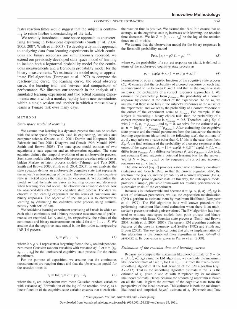
FIG. 1. A: black dots are the reactiontimes from the simulated experiment. Expec-tation maximization (EM) algorithm esti-mates of the reaction-time curve (thick blackcurve) and its 95% confidence intervals(gray area) computed from the reaction-timedata. The vertical line marks trial 24, theIO(0.975) learning trial based only on thereaction-time data. B: the ideal observercurve computed from the analysis of thereaction-time data only crosses 0.975 (hori-zontal line) at trial 24. The horizontal line is0.975. C: the simulated correct (blacksquares) and incorrect (gray squares) trialresponses (top). EM algorithm estimate ofthe learning curve (thick black curve) and its95% confidence interval (gray area) basedon only the binary data. D: ideal observercurve computed from the analysis of thebinary data only. The horizontal line is0.975. There is no IO(0.975) learning trialfrom the analysis of the binary data onlybecause the ideal observer curve drops�0.975 at trial 88.





simulated data, we fit the state-space model in Eqs. 1–4 usingthe EM algorithm in APPENDIX A. We assumed in the modelestimation that the parameter �0 � 0 and � � 1. By so doing,the model used to simulate the data differed from the modelused to analyze the data.

We first analyzed the simulated data assuming that only thereaction times were observed (Fig. 1A). We used this version ofthe state-space model (Eqs. 1 and 2) in the EM algorithmanalysis to estimate the reaction-time curve and its 95% con-fidence intervals (Fig. 1A), the learning trial (A) and the idealobserver curve (B). The simulated observations were highlyvariable relative to the estimated reaction-time curve. Thereaction times varied between 10 and 35 s from trials 1 to 25and thereafter, between 5 and 20 s. The ideal observer curve(Fig. 1B) showed the probability that the reaction on each trialk was less than the reaction time at the outset of the experi-ment, i.e., Pr(rk � r0), for k � 1, . . . , 100. This probabilityincreased steadily from trials 1 to 25, and was 0.975 fromtrial 24 on to the end of the experiment. For this reason, theIO(0.975) learning trial was estimated as trial 24.

We next analyzed the simulated data assuming that only thebinary responses were observed (Fig. 1C). We used this ver-sion of the state-space model (Eqs. 3 and 4) in the EMalgorithm analysis to estimate the learning curve, its 95%confidence intervals (Fig. 1C) and its ideal observer curve (D).This ideal observer curve (Fig. 1D) rose almost monotonicallyfrom trials 1 to 27 where it crossed 0.975 and remained abovethis level of certainty until trial 85. From trial 86 on to trial100, the ideal observer curve decreased almost monotoni-cally to 0.81. Because of this last decrease in performance,the criteria for the IO(9.75) learning trial were not satisfied.These results were consistent with the large number ofcorrect responses from trial 29 to 45 and with the fact thatthere were only five correct responses in trials 85 to 100. Weconcluded that there is no learning trial based on theanalysis of the binary data alone.

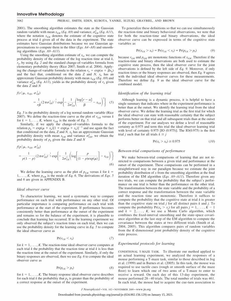
Last we analyzed the simulated data using both the reactiontimes and binary responses (Fig. 2). The combined algorithmestimates of the reaction-time curve (Fig. 2A) and learningcurve (B) resembled approximately their respective continuousand binary estimates. At each trial, the combined algorithm95% confidence intervals for the reaction-time curves (Fig. 2A)

were wider than their reaction-time-only model estimates (Fig.1A). The greater variability in the reaction-time observationsinduced more variability in the learning curve estimate andwider 95% confidence intervals (Fig. 2B) at all trials comparedwith the binary data only estimates (Fig. 1C). The IO(0.975)learning trial was trial 23 for this analysis. This was consistentwith trial 24 suggested by the reaction-time-only analysisrather than the estimate of no-learning trial suggested by theanalysis of the binary data only.

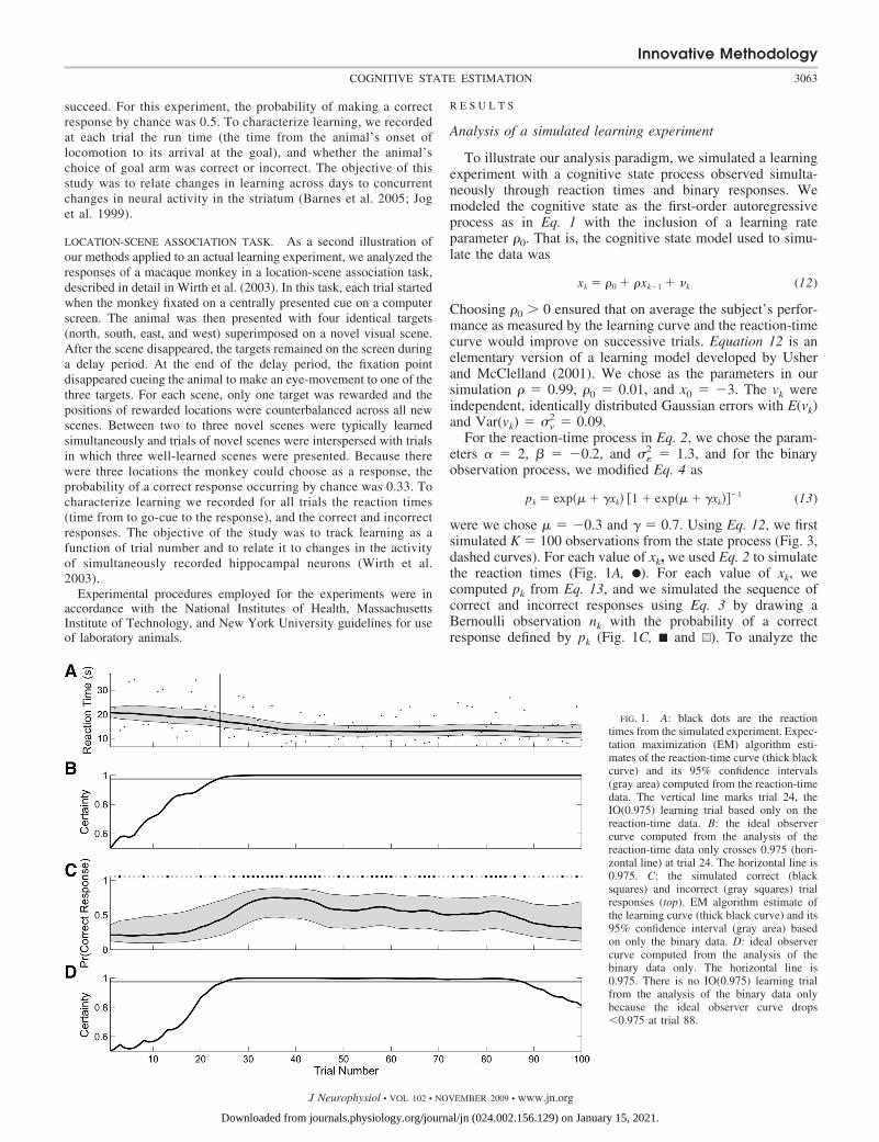
Because the data were simulated, we also compared howwell each of the algorithms estimated the unobservable cogni-tive state (Fig. 3) as a way of assessing goodness of fit. Theestimated cognitive state for the reaction-time-only model(Fig. 3A,—) agreed closely with the true cognitive state (Fig.3A,- - -) from trials 1 to 40. The estimated cognitive stateoverestimated the true cognitive state from trials 41 to 100.These 95% confidence intervals did not cover the true cogni-tive state at trial 60 and between trials 83 and 87. The cognitivestate estimated from the binary observations alone (Fig. 3B,—)overestimated the true cognitive state (Fig. 3B,- - -) from trials1 to 39 and underestimated the true cognitive state from trial 87to 100. Except for trials 1 to 7 and trial 93, these 95%confidence intervals covered the true cognitive state at alltrials.

The combined model estimate of the cognitive state (Fig.3C, —) agreed closely with the true cognitive state (C, - - -).Except for trial 1, these 95% confidence intervals covered thetrue cognitive state for all trials. The performance of thecombined model over the first 40 trials was greatly influencedby the reaction-time data (Fig. 1A). This is the trial range overwhich we observed the largest change in the reaction-timerecordings. The overall shape of the combined model cognitivestate estimate was very close to the binary cognitive stateestimate between trials 29 and 45, where there was a longstring of correct responses (Fig. 1C). Similarly, the downwardtrend in the combined model learning curve from trials 86 to100 occurred because in this range there were only 10 of 15correct responses (Fig. 2C). Overall, the combined modelcognitive state estimate (Fig. 3C) was closer to the true cog-nitive state process than either the reaction-time estimate (A) orthe binary state estimate (B).

FIG. 2. A: black dots are the reactiontimes from the simulated learning experi-ment. EM algorithm estimates of the reac-tion-time curve (black curve) and its 95%confidence intervals (gray area) computedfrom the combined analysis of the reaction-time and binary data. B: the simulated cor-rect (black squares) and incorrect (graysquares) trial responses are shown at the topof this panel. EM algorithm estimate of thecombined analysis learning curve (blackcurve) and its 95% confidence intervals(gray area). The vertical lines mark trial 23,the IO(0.975) learning trial.





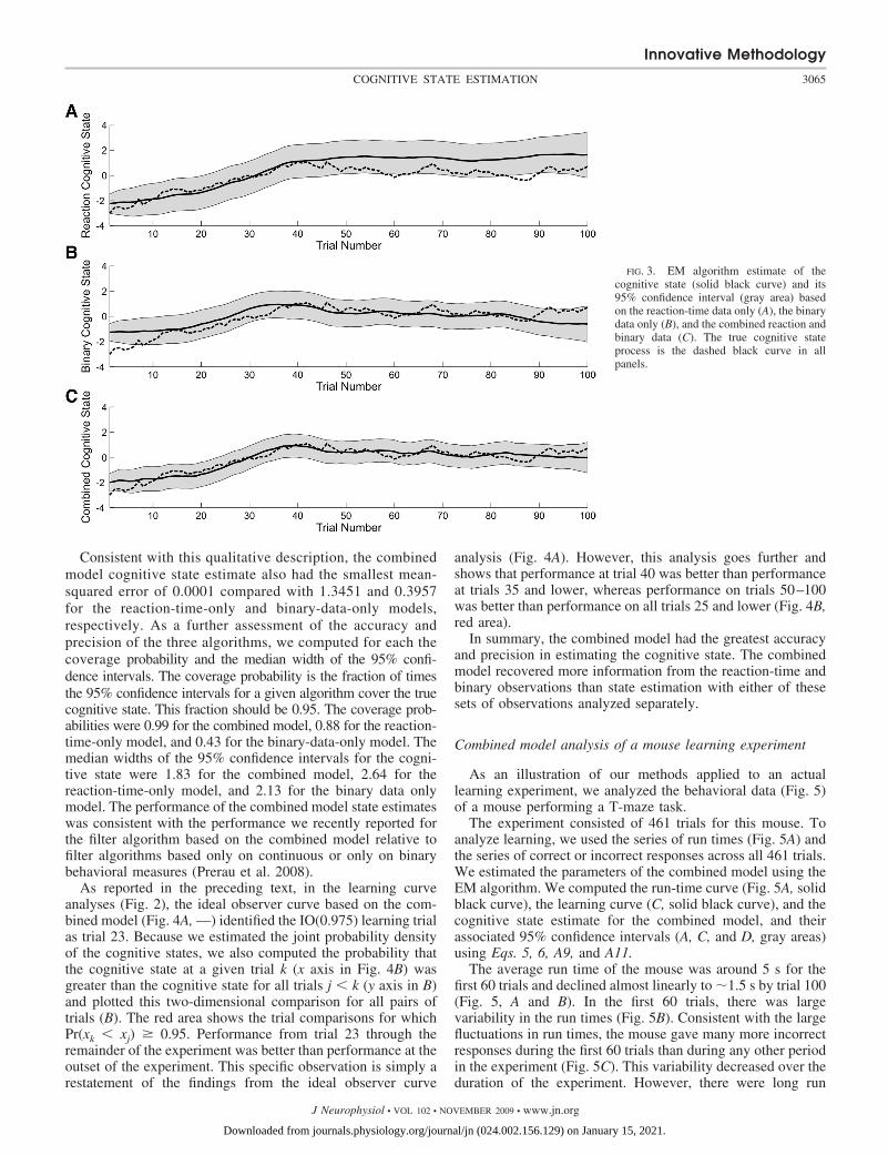
Consistent with this qualitative description, the combinedmodel cognitive state estimate also had the smallest mean-squared error of 0.0001 compared with 1.3451 and 0.3957for the reaction-time-only and binary-data-only models,respectively. As a further assessment of the accuracy andprecision of the three algorithms, we computed for each thecoverage probability and the median width of the 95% confi-dence intervals. The coverage probability is the fraction of timesthe 95% confidence intervals for a given algorithm cover the truecognitive state. This fraction should be 0.95. The coverage prob-abilities were 0.99 for the combined model, 0.88 for the reaction-time-only model, and 0.43 for the binary-data-only model. Themedian widths of the 95% confidence intervals for the cogni-tive state were 1.83 for the combined model, 2.64 for thereaction-time-only model, and 2.13 for the binary data onlymodel. The performance of the combined model state estimateswas consistent with the performance we recently reported forthe filter algorithm based on the combined model relative tofilter algorithms based only on continuous or only on binarybehavioral measures (Prerau et al. 2008).

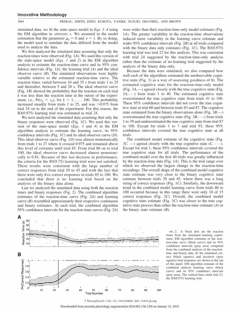
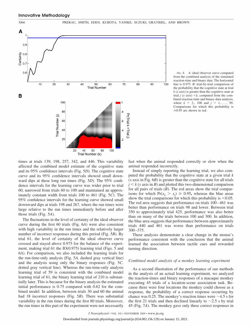
As reported in the preceding text, in the learning curveanalyses (Fig. 2), the ideal observer curve based on the com-bined model (Fig. 4A, —) identified the IO(0.975) learning trialas trial 23. Because we estimated the joint probability densityof the cognitive states, we also computed the probability thatthe cognitive state at a given trial k (x axis in Fig. 4B) wasgreater than the cognitive state for all trials j � k (y axis in B)and plotted this two-dimensional comparison for all pairs oftrials (B). The red area shows the trial comparisons for whichPr(xk � xj) � 0.95. Performance from trial 23 through theremainder of the experiment was better than performance at theoutset of the experiment. This specific observation is simply arestatement of the findings from the ideal observer curve

analysis (Fig. 4A). However, this analysis goes further andshows that performance at trial 40 was better than performanceat trials 35 and lower, whereas performance on trials 50–100was better than performance on all trials 25 and lower (Fig. 4B,red area).

In summary, the combined model had the greatest accuracyand precision in estimating the cognitive state. The combinedmodel recovered more information from the reaction-time andbinary observations than state estimation with either of thesesets of observations analyzed separately.

Combined model analysis of a mouse learning experiment

As an illustration of our methods applied to an actuallearning experiment, we analyzed the behavioral data (Fig. 5)of a mouse performing a T-maze task.

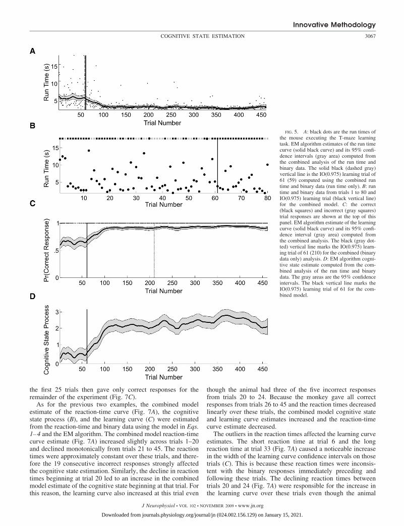
The experiment consisted of 461 trials for this mouse. Toanalyze learning, we used the series of run times (Fig. 5A) andthe series of correct or incorrect responses across all 461 trials.We estimated the parameters of the combined model using theEM algorithm. We computed the run-time curve (Fig. 5A, solidblack curve), the learning curve (C, solid black curve), and thecognitive state estimate for the combined model, and theirassociated 95% confidence intervals (A, C, and D, gray areas)using Eqs. 5, 6, A9, and A11.

The average run time of the mouse was around 5 s for thefirst 60 trials and declined almost linearly to 1.5 s by trial 100(Fig. 5, A and B). In the first 60 trials, there was largevariability in the run times (Fig. 5B). Consistent with the largefluctuations in run times, the mouse gave many more incorrectresponses during the first 60 trials than during any other periodin the experiment (Fig. 5C). This variability decreased over theduration of the experiment. However, there were long run

FIG. 3. EM algorithm estimate of thecognitive state (solid black curve) and its95% confidence interval (gray area) basedon the reaction-time data only (A), the binarydata only (B), and the combined reaction andbinary data (C). The true cognitive stateprocess is the dashed black curve in allpanels.





times at trials 139, 198, 257, 342, and 446. This variabilityaffected the combined model estimate of the cognitive stateand its 95% confidence intervals (Fig. 5D). The cognitive statecurve and its 95% confidence intervals showed small down-ward dips at these long run times (Fig. 5D). The 95% confi-dence intervals for the learning curve was wider prior to trial60, narrowed from trials 60 to 100 and maintained an approx-imately constant width from trials 100 to 461 (Fig. 5C). The95% confidence intervals for the learning curve showed smalldownward dips at trials 198 and 267, where the run times werelarge relative to the run times immediately before and afterthose trials (Fig. 5A).

The fluctuations in the level of certainty of the ideal observercurve during the first 60 trials (Fig. 6A) were also consistentwith high variability in the run times and the relatively largernumber of incorrect responses during this period (Fig. 5B). Bytrial 61, the level of certainty of the ideal observer curvecrossed and stayed above 0.975 for the balance of the experi-ment, making trial 61 the IO(0.975) learning trial (Figs. 5 and6A). For comparison, we also included the learning trials forthe run-time-only analysis (Fig. 5A, dashed gray vertical line)and the analysis using only the binary responses (Fig. 5C,dotted gray vertical line). Whereas the run-time-only analysislearning trial of 59 is consistent with the combined modellearning trial of 61, the binary learning trial of 210 is substan-tially later. This is because for the binary analysis the estimatedinitial performance is 0.75 compared with 0.62 for the com-bined model. In addition, between trials 30 and 60 the animalhad 18 incorrect responses (Fig. 5B). There was substantialvariability in the run times during the first 80 trials. Moreover,the run times in this part of the experiment were not necessarily

fast when the animal responded correctly or slow when theanimal responded incorrectly.

Instead of simply reporting the learning trial, we also com-puted the probability that the cognitive state at a given trial k(x axis in Fig. 6B) is greater than the cognitive state for all trialsj � k (y axis in B) and plotted this two-dimensional comparisonfor all pairs of trials (B). The red areas show the trial compar-isons for which Pr(xk xj) � 0.95, whereas the blue areasshow the trial comparisons for which this probability is �0.05.The red area suggests that performance on trials 100–461 wasbetter than performance on trials 98 and lower. Between trial350 to approximately trial 425, performance was also betterthan on many of the trials between 100 and 300. In addition,the blue area suggests that performance between approximatelytrials 440 and 461 was worse than performance on trials300–375.

These analyses demonstrate a clear change in the mouse’sperformance consistent with the conclusion that the animallearned the association between tactile cues and rewardedturning direction.

Combined model analysis of a monkey learning experiment

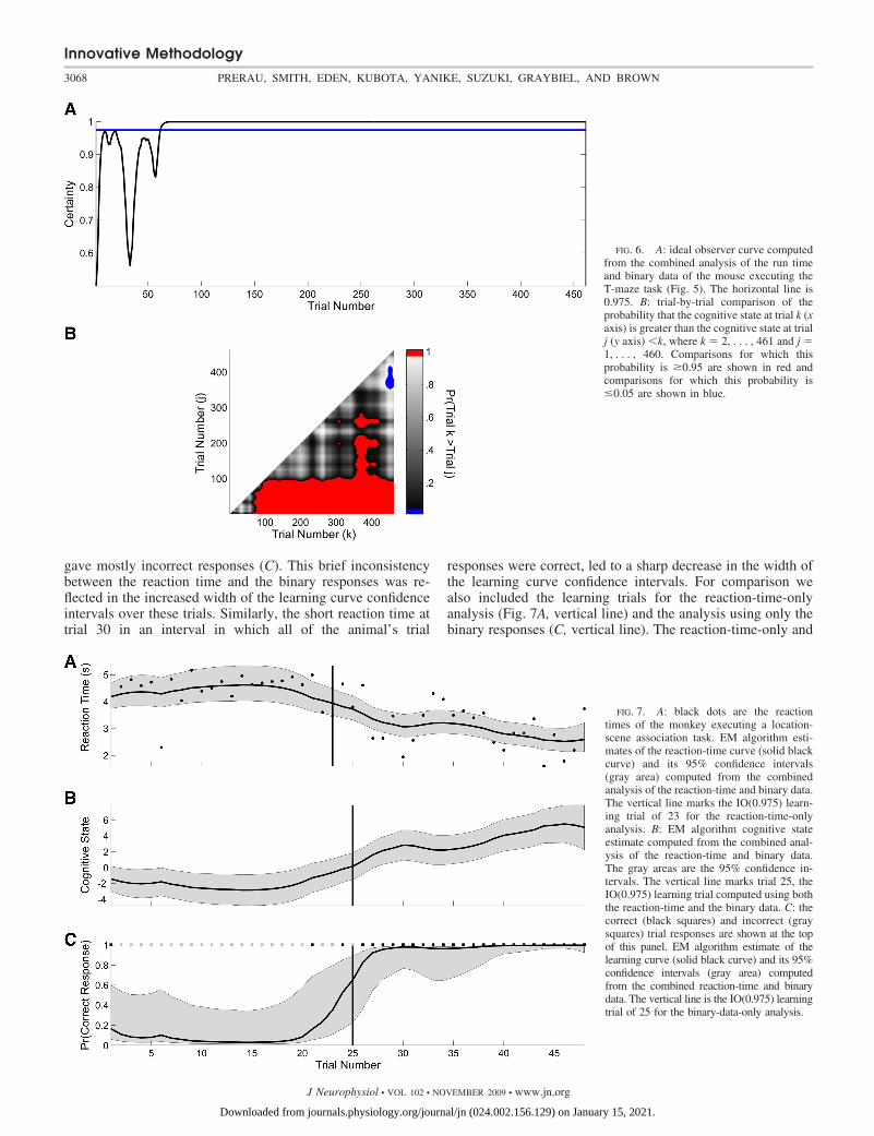
As a second illustration of the performance of our methodsin the analysis of an actual learning experiment, we analyzedthe reaction-times and binary responses of a macaque monkeyexecuting 45 trials of a location-scene association task. Be-cause there were four locations the monkey could choose as aresponse, the probability of a correct response occurring bychance was 0.25. The monkey’s reaction times were 4.5 s forthe first 21 trials and then declined linearly to 2.5 s by trial45 (Fig. 7A). The monkey gave only three correct responses in

FIG. 4. A: ideal observer curve computedfrom the combined analysis of the simulatedreaction-time and binary data. The horizontalline is 0.975. B: trial-by-trial comparison ofthe probability that the cognitive state at trialk (x axis) is greater than the cognitive state attrial j (y axis) �k, computed from the com-bined reaction-time and binary-data analysis,where k � 2,, 100 and j � 1, . . . , 99.Comparisons for which this probability is�0.95 are shown in red.





the first 25 trials then gave only correct responses for theremainder of the experiment (Fig. 7C).

As for the previous two examples, the combined modelestimate of the reaction-time curve (Fig. 7A), the cognitivestate process (B), and the learning curve (C) were estimatedfrom the reaction-time and binary data using the model in Eqs.1–4 and the EM algorithm. The combined model reaction-timecurve estimate (Fig. 7A) increased slightly across trials 1–20and declined monotonically from trials 21 to 45. The reactiontimes were approximately constant over these trials, and there-fore the 19 consecutive incorrect responses strongly affectedthe cognitive state estimation. Similarly, the decline in reactiontimes beginning at trial 20 led to an increase in the combinedmodel estimate of the cognitive state beginning at that trial. Forthis reason, the learning curve also increased at this trial even

though the animal had three of the five incorrect responsesfrom trials 20 to 24. Because the monkey gave all correctresponses from trials 26 to 45 and the reaction times decreasedlinearly over these trials, the combined model cognitive stateand learning curve estimates increased and the reaction-timecurve estimate decreased.

The outliers in the reaction times affected the learning curveestimates. The short reaction time at trial 6 and the longreaction time at trial 33 (Fig. 7A) caused a noticeable increasein the width of the learning curve confidence intervals on thosetrials (C). This is because these reaction times were inconsis-tent with the binary responses immediately preceding andfollowing these trials. The declining reaction times betweentrials 20 and 24 (Fig. 7A) were responsible for the increase inthe learning curve over these trials even though the animal

FIG. 5. A: black dots are the run times ofthe mouse executing the T-maze learningtask. EM algorithm estimates of the run timecurve (solid black curve) and its 95% confi-dence intervals (gray area) computed fromthe combined analysis of the run time andbinary data. The solid black (dashed gray)vertical line is the IO(0.975) learning trial of61 (59) computed using the combined runtime and binary data (run time only). B: runtime and binary data from trials 1 to 80 andIO(0.975) learning trial (black vertical line)for the combined model. C: the correct(black squares) and incorrect (gray squares)trial responses are shown at the top of thispanel. EM algorithm estimate of the learningcurve (solid black curve) and its 95% confi-dence interval (gray area) computed fromthe combined analysis. The black (gray dot-ted) vertical line marks the IO(0.975) learn-ing trial of 61 (210) for the combined (binarydata only) analysis. D: EM algorithm cogni-tive state estimate computed from the com-bined analysis of the run time and binarydata. The gray areas are the 95% confidenceintervals. The black vertical line marks theIO(0.975) learning trial of 61 for the com-bined model.





gave mostly incorrect responses (C). This brief inconsistencybetween the reaction time and the binary responses was re-flected in the increased width of the learning curve confidenceintervals over these trials. Similarly, the short reaction time attrial 30 in an interval in which all of the animal’s trial

responses were correct, led to a sharp decrease in the width ofthe learning curve confidence intervals. For comparison wealso included the learning trials for the reaction-time-onlyanalysis (Fig. 7A, vertical line) and the analysis using only thebinary responses (C, vertical line). The reaction-time-only and

FIG. 6. A: ideal observer curve computedfrom the combined analysis of the run timeand binary data of the mouse executing theT-maze task (Fig. 5). The horizontal line is0.975. B: trial-by-trial comparison of theprobability that the cognitive state at trial k (xaxis) is greater than the cognitive state at trialj (y axis) �k, where k � 2, . . . , 461 and j �1, . . . , 460. Comparisons for which thisprobability is �0.95 are shown in red andcomparisons for which this probability is�0.05 are shown in blue.

FIG. 7. A: black dots are the reactiontimes of the monkey executing a location-scene association task. EM algorithm esti-mates of the reaction-time curve (solid blackcurve) and its 95% confidence intervals(gray area) computed from the combinedanalysis of the reaction-time and binary data.The vertical line marks the IO(0.975) learn-ing trial of 23 for the reaction-time-onlyanalysis. B: EM algorithm cognitive stateestimate computed from the combined anal-ysis of the reaction-time and binary data.The gray areas are the 95% confidence in-tervals. The vertical line marks trial 25, theIO(0.975) learning trial computed using boththe reaction-time and the binary data. C: thecorrect (black squares) and incorrect (graysquares) trial responses are shown at the topof this panel. EM algorithm estimate of thelearning curve (solid black curve) and its 95%confidence intervals (gray area) computedfrom the combined reaction-time and binarydata. The vertical line is the IO(0.975) learningtrial of 25 for the binary-data-only analysis.





the binary-only learning-trial estimates of trials 23 and 25,respectively, were in close agreement with the combinedmodel estimate of 25.

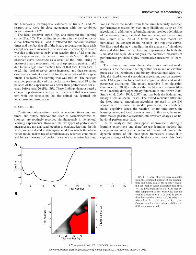
The ideal observer curve (Fig. 8A) mirrored the learningcurve (Fig. 7C). The decline in certainty in the ideal observercurve between trials 1 and 5 reflected the constant reactiontimes and the fact that all of the binary responses on these trialsexcept one were incorrect. The increase in certainty at trial 6was due to the anomalously short reaction time of 2.1 s on thattrial despite an incorrect answer. From trials 6 to 15, the idealobserver curve decreased as a result of the initial string ofincorrect binary responses, with a sharp upward peak at trial 6due to the single short reaction time at that trial. From trial 16to 27, the ideal observer curve increased, and then remainedessentially constant close to 1 for the remainder of the exper-iment. The IO(0.975) learning trial was trial 25. The betweentrial comparison showed that performance from trial 28 to thebalance of the experiment was better than performance for alltrials before trial 26 (Fig. 8B). These findings demonstrated achange in performance across the experiment that was consis-tent with the conclusion that the animal had learned thislocation-scene association.

D I S C U S S I O N

Continuous observations, such as reaction times and runtimes, and binary observations, such as correct/incorrect re-sponses, are routinely recorded simultaneously in behaviorallearning experiments. However, the two types of performancemeasures are not analyzed together to evaluate learning. In thiswork, we introduced a state-space model in which the obser-vation model makes use of simultaneously recorded continuousand binary measures of performance to characterize learning.

We estimated the model from these simultaneously recordedperformance measures by maximum likelihood using an EMalgorithm. In addition to reformulating our previous definitionsof the learning curve, the ideal observer curve, and the learningtrial (Smith et al. 2004) in terms of the new model, weintroduced the concept of the reaction- and run-time curves.We illustrated the new paradigm in the analysis of simulateddata and data from actual learning experiments. In both thesimulated and actual data analyses, the combined measures ofperformance provided highly informative measures of learn-ing.

The technical innovation that enabled this combined modelanalysis is the recursive filter algorithm for mixed observationprocesses (i.e., continuous and binary observations) (Eqs. A4–A8), the fixed-interval smoothing algorithm, and an approxi-mate EM algorithm for combined cognitive state and modelparameter estimation. The mixed recursive filter algorithm(Prerau et al. 2008) combines the well-known Kalman filterwith a recently developed binary filter (Smith and Brown 2003;Smith et al. 2004, 2005, 2007) and has both the Kalman andbinary filters as special cases. The mixed recursive filter andthe fixed-interval smoothing algorithm are used in the EMalgorithm to estimate the model parameters, the combinedmodel cognitive states, the reaction- or run-time curve, thelearning curve, and ideal observer curve. In this way, the mixedfilter makes possible a dynamic, multivariate analysis of be-havioral performance data.

Unlike analyses that presuppose improvement during alearning experiment and therefore use learning models thatchange monotonically as a function of time or trial number, thedynamic nature of this state-space framework allows it tocapture a range of behaviors. In the current work, this flexi-

FIG. 8. A: ideal observer curve computedfrom the combined analysis of the reaction-time and binary data of the monkey execut-ing the location-scene association task (Fig.7). The horizontal line is 0.975. B: trial-by-trial comparison of the probability that thecognitive state at trial k (x axis) is greaterthan the cognitive state at trial j (y axis) � k,where k � 2, . . . , 45 and j � 1, . . . , 44.Comparisons for which this probability is �0.95 are shown in red.





bility is illustrated by estimated performance indices that ini-tially declined in the first half of the experiment, then improvedin the latter half (Fig. 7).

How well does the model work?

In situations where the estimated cognitive state can becompared with a true cognitive state, standard goodness-of-fitprocedures can be applied. However, in the actual data exam-ples we considered, the true cognitive state was unknown.Therefore a standard goodness-of-fit analysis was not possibleand alternative approaches had to be considered. For thisreason, to assess performance, we conducted a simulation inwhich the model used to simulate the data differed from themodel used in the estimation. We demonstrated that despitethis difference, there was a highly accurate recovery of theunderlying cognitive state process. While this result alone isnot definitive, it suggests that the state-space model used in theanalysis can differ from the dynamical model of the underlyingcognitive process. Our approach provides a plausible way tofuse information from two different sources related by acommon state process. As another performance measure, wecould also use standard model selection approaches such asAIC and BIC to choose among a class of models that areappropriate for the data. In this case, we could compare thedata description given by the models that had the smallest AICand BIC. Despite use of these performance measures andmodel selection criteria, the interpretation of the model anal-ysis in the context of the particular problem must also beplausible to infer that the particular model provides a reason-able data summary. A practical test of this is the extent towhich the model can be used to design more efficient experi-ments and to conduct statistical power analyses. By makingmore efficient use of the data, we may be able to reduce theamount of recording required to estimate specific features ofthe learning process. Although we did not consider theseexperimental design issues here, results along these lines usingstate-space models for behavioral data have been reported inSmith et al. (2005).

Future directions

Several extensions of the current work are possible includingdeveloping models that can represent binary and continuousmeasures of performance along with simultaneously recordedspiking activity from multiple neurons, representing the cog-nitive state as a multidimensional rather than one-dimensional(Smith et al. 2006; Usher and McClelland 2001), and formu-lating the models in continuous rather than in discrete time. Inaddition, developing more complex, potentially nonmonotonicdescriptions of the relationships between the cognitive statesand the observations could yield models that offer insights intoimportant phenomena such as over-training, behavioral strate-gies, and strategy switching (Smith et al. 2007). In this way,these more in-depth models would provide an opportunity tolink our state-space methods to current work on learningstrategies (Chater and Oaksford 2008; Dayan and Yu 2002;Gallistel 2008; Kakade and Dayan 2002; Smith et al. 2006;Usher and McClelland 2001).

In principle, the generalized observation models and thestate models can be fit to experimental data using the EM

algorithm paradigm described here. To carry out these compu-tations, the E-step would be most efficiently computed usingMonte Carlo methods such as those described in Chan andLedolter (1995). However, models such as these are nowreadily analyzed with sequential Monte Carlo (Doucet et al.2001; Ergun et al. 2007) and Bayesian Markov Chain MonteCarlo methods (Gelman 2004). In the sequential Monte Carloapproach, the mixed filter algorithm could serve as a proposaldensity (Ergun et al. 2007).

Our approach provides a solution to the important problemof combining information from different measurement types toimprove state estimation. Therefore it may be applied in theanalysis of other problems in neuroscience in which differentmeasurement types are being simultaneously recorded to studya neural system. For example, behavioral performance mea-sures are frequently recorded with neural spike trains in learn-ing experiments to establish neural correlates of behavior(Barnes et al. 2005; Wirth et al. 2003). As suggested by themodel generalizations discussed in the preceding text, ourparadigm offers an approach to establishing such correlatesbased on a joint model of the two measurement types (Smith etal. 2007). Second, neurophysiological experiments commonlyrecord multiple neural spike trains and local field potentialssimultaneously. Our paradigm may be used to develop dy-namic approaches to analyzing the properties of a particularneural system by conducting a combined analysis of its mea-surements. Such algorithms could also make it possible to usesimultaneously recorded ensemble neural spiking activity andlocal field potentials to improve control of neural prostheticdevices and brain machine interfaces (Hochberg et al. 2006;Srinivasan et al. 2007). Finally, a central focus of currentfunctional neuroimaging research is the development of toolsfor multimodal imaging using functional magnetic resonanceimaging, electroencephalography, magnetoencephalography,and diffuse optical tomography. This means conducting exper-iments in which imaging is performed with two or more ofthese modalities, simultaneously or in sequence, so that theinformation from the different sources can be combined (Liu etal. 1998; Molins et al. 2008). The concepts underlying ourapproach could be applied to this problem as well. Thesetheoretical and applied extensions will be the topics of futureinvestigations.

A P P E N D I X A . D E R I V A T I O N O F T H E

E M A L G O R I T H M

Use of the EM algorithm to compute the maximum likelihood esti-mates of � requires us to maximize the expectation of the complete datalog-likelihood. The complete data likelihood is the joint probabilitydensity of Z, N, and x, which for our model is

p�Z, N, x�� k�1

K

pknk�1 pk�

1�nk

� �k�1

K

�2 � �2��

12 exp�� 2� �

2��1�zk � �xk�2�

� �k�1

K

�2 � �2��

12 exp�� 2� �

2��1�xk �xk�1�2� (A1)

where the first term on the right of Eq. A1 is defined by the Bernoulliprobability mass function in Eq. 3, the second term is defined by theGaussian probability density in Eq. 2, and the third term is the jointprobability density of the state process defined by the Gaussian model





in Eq. 13. At iteration (�� 1) of the algorithm, we compute in theE-step the expectation of the complete data log likelihood given theresponses N and Z across the K trials and �(�) � (�(�), ��

2(�), �(�),�(�), �v

(�), x0(�)), the parameter estimates from iteration �, which are

defined as

E-step

E�log�p�Z, N, x � �� Z, N, ��

� E�k�1

K

�nk log�pk�1 pk��1� � log�1 pk�� Z, N, ��

� E� 1

2K log�2 � �

2� �2� �2��1

k�1

K

�zk � �xk�2 � Z, N, ��

� E� 1

2K log�2 � �

2� �2� �2��1

k�1

K

�xk �xk�1�2 � Z, N, ��

(A2)

To evaluate the E-step we have to consider terms such as

xk�K � E�xk Z, N, ��Wk�K � E�xk

2 Z, N, ��Wk�1,k�K � E�xkxk�1 Z, N, �� (A3)

for k � 1, . . . , K where the notation k�j denotes the expectation of thestate variable at k given the responses up to time j. To compute thesequantities efficiently, we follow a strategy first suggested by Shum-way and Stoffer (1982) for linear Gaussian state and observationmodels and decompose the E-step into three parts: a nonlinear recur-sive filter algorithm to compute xk�k, a fixed interval smoothingalgorithm to estimate xk�K, and a state-space covariance algorithm toestimate Wk�K and Wk,k�1�K.

Filter algorithm

Given �(�) we can first compute recursively the state variable, xk�kand its variance, �k�k

2 . We accomplish this using the following non-linear filter algorithm for combined continuous and binary processesas derived in Prerau et al. (2008)

xk�k�1 � ��xk�1�k�1 (A4)

� k�k�12 � ��2� k�1�k�1

2 � � �2�� (A5)

Ck � ��2� k�k�12 � � �

2��1� k�k�12 (A6)

xk�k � xk�k�1 � Ck��zk �� xk�k�1� � � �2��nk pk�k�� (A7)

� k�k2 � �� k�k�1

2 ��1 � pk�k�1 pk�k� � �� 2��1��2��1 (A8)

for k � 1, . . . , K.

Fixed interval smoothing algorithm

Given the sequence of posterior mode estimates xk�k (Eq. A7) andthe variance �k�k

2 (Eq. A8), we use the fixed-interval smoothingalgorithm (Smith et al. 2004) to compute xk�k and �k�K. This smoothingalgorithm is

xk�K � xk�k � Ak�xk�1�K xk�1�k� (A9)

Ak � � k�k2 �� k�1�k

2 ��1 (A10)

� k�K2 � � k�k

2 � Ak2�� k�1�k

2 � k�1�K2 � (A11)

for k � K � 1, . . . , 1 and initial conditions xk�K and �k�K2 .

State-space covariance algorithm

The covariance estimate, �k,u�K, can be computed from the state-space covariance algorithm (Dejong and Mackinnon 1988) and isgiven as

�k,u�k � Ak�k�1,u�k (A12)

for 1 � k � u � K.The variance and covariance terms required for the E-step are

Wk�K � � k�K2 � xk�K

2 (A13)

Wk�1,k�K � �k�1,k�K � xk�1�kxk�K (A14)

In the M-step, we maximize the expected value of the complete datalog likelihood in Eq. A2 with respect to �(��1) giving

M-step

��1� � k�1

K

Wk�1,k�K� k�1

K

Wk�1�K��1

(A15)

x0��1� � �x1�k (A16)

� �2��1� � K�1

k�1

K

zk2 � K�2��1�

� �2��1�k�1

K

Wk�K 2��1�k�1

K

zk

2��1�k�1

K

xk�Kzk � 2��1��1�k�1

K

xk�K (A17)

��1�

��1� � � K k�1

K

xk�K

k�1

K

xk�K k�1

K

Wk�K�

�1

k�1

K

zk

k�1

K

xk�Kzk� (A18)

� �2 � K�1

k�1

K

�Wk�K 2�Wk�1,k�K � �2Wk�1�K� (A19)

The algorithm is iterated between the E-step (Eq. A2) and theM-step (Eqs. A16 and A17) using the filter algorithm, the fixedinterval smoothing algorithm and the state covariance algorithm toevaluate the E-step. The maximum likelihood estimate of �̂ � �( ).The convergence criteria for the algorithm are those used in Smith andBrown (2003). The fixed-interval-smoothing algorithm evaluated atthe maximum likelihood estimate of � (Eqs. A10–A12) together withEqs. 5 and 6 give the maximum likelihood or empirical Bayes’estimates of the reaction-time curves and the learning curve.

A P P E N D I X B . P R O B A B I L I T Y D E N S I T I E S O F T H E

R E A C T I O N - T I M E A N D T H E L E A R N I N G C U R V E S

To compute the probability density of the reaction time rk from theposterior probability density of the state process xk, we use thestandard change-of-variables formula (Rice 2007)

p�rk � Z, N, �̂� � p�xk � Z, �̂�� dxk

drk

� (B1)

where p(xk�Z, N, �̂) is the Gaussian probability density mean xk�K andvariance �k�K

2 . Applying (Eq. A19) by substituting xk � ��1(logrk ��) into p(xk�Z, N, �̂) and multiplying by dxk

/drk� (�rk)

�1 yields thelognormal probability density for the reaction-time curve in Eq. 5.From the approximate posterior probability density of xk, we can alsocompute the probability density of pk by using Eq. 4 and the change-of-variable formula





p�pk�Z, N, �̂� � p�xk�Z, N, �̂�� dxk

dpk

� (B2)

Hence setting xk �{log[pk(1 � pk)�1] � �} in p(xk�Z, N, �̂) and

computing dxk/dpk � [pk(1 � pk)]�1, we obtain Eq. 6.

G R A N T S

Support was provided by National Institutes of Health Grants DA-015644to E. N. Brown and W. Suzuki, DPI0D003646, MH-59733 and MH-071847 toE. N. Brown, and P50 NS-38372 to A. M. Graybiel.

R E F E R E N C E S

Barnes TD, Kubota Y, Hu D, Jin DZZ, Graybiel AM. Activity of striatalneurons reflects dynamic encoding and recoding of procedural memories.Nature 437: 1158–1161, 2005.

Chan KS, Ledolter J. Monte-Carlo Em estimation for time-series modelsinvolving counts. J Am Stat Assoc 90: 242–252, 1995.

Chater N, Oaksford M. The Probabilistic Mind: Prospects for BayesianCognitive Science. Oxford, UK: Oxford Univ. Press, 2008.

Dayan P, Yu A. Expected and unexpected uncertainty: Ach and NE in theneocortex. In: Advances in Neural Information Processing Sysytems, editedby Dietterich T, Becker S, Ghahramani Z. Cambridge, MA: MIT Press,2002, p. 189–196.

Dejong P, Mackinnon MJ. Covariances for smoothed estimates in state-spacemodels. Biometrika 75: 601–602, 1988.

Dempster AP, Laird NM, Rubin DB. Maximum likelihood from incompletedata via Em algorithm. J Roy Stat Soc B Met 39: 1–38, 1977.

Dias R, Robbins TW, Roberts AC. Dissociable forms of inhibitory controlwithin prefrontal cortex with an analog of the Wisconsin Card Sort Test:restriction to novel situations and independence from “on-line” processing.J Neurosci 17: 9285–9297, 1997.

Doucet A, De Freitas N, Gordon N. Sequential Monte Carlo Methods inPractice. New York: Springer, 2001.

Durbin J, Koopman SJ. Time Series Analysis by State Space Methods.Oxford, UKk: Oxford Univ. Press, 2001.

Dusek JA, Eichenbaum H. The hippocampus and memory for orderlystimulus relations. Proc Natl Acad Sci USA 94: 7109–7114, 1997.

Ergun A, Barbieri R, Eden UT, Wilson MA, Brown EN. Construction ofpoint process adaptive filter algorithms for neural systems using sequentialMonte Carlo methods. IEEE Trans Biomed Eng 54: 419–428, 2007.

Fahrmeir L, Tutz G. Multivariate Statistical Modelling Based on GeneralizedLinear Models. New York: Springer, 2001.

Fox MT, Barense MD, Baxter MG. Perceptual attentional set-shifting isimpaired in rats with neurotoxic lesions of posterior parietal cortex. J Neu-rosci 23: 676–681, 2003.

Gallistel CR. Learning and representation. In: Learning Theory and Behavior.Learning and Memory- A Comprehensive Reference, edited by Byrne J.Oxford: Elsevier, 2008, vol. 1, p. 227–242.

Gallistel CR, Fairhurst S, Balsam P. The learning curve: implications of aquantitative analysis. Proc Natl Acad Sci USA 101: 13124–13131, 2004.

Gelman A. Bayesian Data Analysis. Boca Raton, FL: Chapman and Hall/CRC, 2004.

Hochberg LR, Serruya MD, Friehs GM, Mukand JA, Saleh M, CaplanAH, Branner A, Chen D, Penn RD, Donoghue JP. Neuronal ensemblecontrol of prosthetic devices by a human with tetraplegia. Nature 442:164–171, 2006.

Jog MS, Kubota Y, Connolly CI, Hillegaart V, Graybiel AM. Buildingneural representations of habits. Science 286: 1745–1749, 1999.

Kakade S, Dayan P. Acquisition and extinction in autoshaping. Psychol Rev109: 533–544, 2002.

Kitagawa G, Gersch W. Smoothness Priors Analysis of Time Series. NewYork: Springer, 1996.

Law JR, Flanery MA, Wirth S, Yanike M, Smith AC, Frank LM, SuzukiWA, Brown EN, Stark CEL. Functional magnetic resonance imagingactivity during the gradual acquisition and expression of paired-associatememory. J Neurosci 25: 5720–5729, 2005.

Liu AK, Belliveau JW, Dale AM. Spatiotemporal imaging of human brainactivity using functional MRI constrained magnetoencephalography data:Monte Carlo simulations. Proc Natl Acad Sci USA 95: 8945–8950, 1998.

Mendel JM. Lessons in Estimation Theory for Signal Processing, Communi-cations, and Control. Englewood Cliffs, NJ: Prentice Hall PTR, 1995.

Molins A, Stufflebeam SM, Brown EN, Hamalainen MS. Quantification ofthe benefit from integrating MEG and EEG data in minimum l(2)-normestimation. Neuroimage 42: 1069–1077, 2008.

Prerau MJ, Smith AC, Eden UT, Yanike M, Suzuki WA, Brown EN. Amixed filter algorithm for cognitive state estimation from simultaneouslyrecorded continuous and binary measures of performance. Biol Cybern 99:1–14, 2008.

Rice JA. Mathematical Statistics and Data Analysis. Belmont, CA: Thomson/Brooks/Cole, 2007.

Roman FS, Simonetto I, Soumireumourat B. Learning and memory ofodor-reward associatio—selective impairment following horizontal diagonalband lesions. Behav Neurosci 107: 72–81, 1993.

Rondi-Reig L, Libbey M, Eichenbaum H, Tonegawa S. CA1-specificN-methyl-d-aspartate receptor knockout mice are deficient in solving anonspatial transverse patterning task. Proc Natl Acad Sci USA 98: 3543–3548, 2001.

Shumway R, Stoffer D. An approach to time series smoothing and forecastingusing the EM algorithm. J Time Ser Anal 3: 253–264, 1982.

Siegel S, Castellan NJ. Nonparametric Statistics for the Behavioral Sciences.New York: McGraw-Hill, 1988.

Smith AC, Brown EN. Estimating a state-space model from point processobservations. Neural Comput 15: 965–991, 2003.

Smith AC, Frank LM, Wirth S, Yanike M, Hu D, Kubota Y, Graybiel AM,Suzuki WA, Brown EN. Dynamic analysis of learning in behavioralexperiments. J Neurosci 24: 447–461, 2004.

Smith AC, Stefani MR, Moghaddam B, Brown EN. Analysis and design ofbehavioral experiments to characterize population learning. J Neurophysiol93: 1776–1792, 2005.

Smith AC, Wirth S, Suzuki WA, Brown EN. Bayesian analysis of inter-leaved learning and response bias in behavioral experiments. J Neurophysiol97: 2516–2524, 2007.

Smith MA, Ghazizadeh A, Shadmehr R. Interacting adaptive processes withdifferent time scales underlie short-term motor learning. Plos Biol 4:1035–1043, 2006.

Srinivasan L, Eden UT, Mitter SK, Brown EN. General-purpose filterdesign for neural prosthetic devices. J Neurophysiol 98: 2456–2475, 2007.

Stefani MR, Groth K, Moghaddam B. Glutamate receptors in the rat medialprefrontal cortex regulate set-shifting ability. Behav Neurosci 117: 728–737,2003.

Usher M, McClelland JL. The time course of perceptual choice: the leaky,competing accumulator model. Psychol Rev 108: 550–592, 2001.

Whishaw IQ, Tomie JA. Acquisition and retention by hippocampal rats ofsimple, conditional, and configural tasks using tactile and olfactory cues—implications for hippocampal function. Behav Neurosci 105: 787–797,1991.

Williams ZM, Eskandar EN. Selective enhancement of associative learningby microstimulation of the anterior caudate. Nat Neurosci 9: 562–568, 2006.

Wirth S, Yanike M, Frank LM, Smith AC, Brown EN, Suzuki WA. Singleneurons in the monkey hippocampus and learning of new associations.Science 300: 1578–1581, 2003.

Wise SP, Murray EA. Role of the hippocampal system in conditional motorlearning: mapping antecedents to action. Hippocampus 9: 101–117, 1999.





Documents

Characterizing Learning by Simultaneous Analysis of