Characterizing ions in solution by NMR methods MARIANNE GIESECKE

KTH Royal Institute of Technology School of Chemical Science and Engineering Department of Chemistry Applied Physical Chemistry SE-100 44 Stockholm, Sweden

  

ii  

Copyright © Marianne Giesecke, 2014. All rights reserved. No parts of this thesis may be reproduced without permission from the author. TRITA-CHE Report 2014:29 ISSN 1654-1081 ISBN 978-91-7595-208-6 Akademisk avhandling som med tillstånd av Kungliga Tekniska Högskolan i Stockholm framlägges till offentlig granskning för avläggandet av teknologie doktorsexamen fredagen den 12 september kl 14:00 i sal F3, KTH, Lindstedtsvägen 26, Stockholm.

  

iii  

 

 

To my parents,

To Fredrik and Isolde,

 

 

 

 

 

 

 

 

  

iv  

 

 

 

 

  

v  

Abstract

NMR experiments performed under the effect of electric fields, either continuous or pulsed, can provide quantitative parameters related to ion association and ion transport in solution. Electrophoretic NMR (eNMR) is based on a diffusion pulse-sequence with electric fields applied in the form of pulses. Magnetic field gradients enable the measurement of the electrophoretic mobility of charged species, a parameter that can be related to ionic association.

The effective charge of the tetramethylammonium cation ion in water, dimethylsulphoxide (DMSO), acetonitrile, methanol and ethanol was estimated by eNMR and diffusion measurements and compared to the value predicted by the Debye-Hückel-Onsager limiting law. The difference between the predicted and measured effective charge was attributed to ion pairing which was found to be especially significant in ethanol.

The association of a large set of cations to polyethylene oxide (PEO) in methanol, through the ion-dipole interaction, was quantified by eNMR. The trends found were in good agreement with the scarce data from other methods. Significant association was found for cations that have a surface charge density below a critical value. For short PEO chains, the charge per monomer was found to be significantly higher than for longer PEO chains when binding to the same cations. This was attributed to the high entropy cost required to rearrange a long chain in order to optimize the ion-dipole interactions with the cations. Moreover, it was suggested that short PEO chains may exhibit distinct binding modes in the presence of different cations, as supported by diffusion measurements, relaxation measurements and chemical shift data.

The protonation state of a uranium (VI)-adenosine monophosphate (AMP) complex in aqueous solution was measured by eNMR in the alkaline pH range. The question whether or not specific oxygens in the ligand were protonated was resolved by considering the possible association of other species present in the solution to the complex.

The methodology of eNMR was developed through the introduction of a new pulse-sequence which suppresses artifactual flow effects in highly conductive samples.

In another experimental setup, using NMR imaging, a constant current was applied to a lithium ion (Li ion) battery model. Here, 7Li spin-echo imaging was used to

  

vi  

probe the spin density in the electrolyte and thus visualize the development of Li+ concentration gradients. The Li+ transport number and salt diffusivity were obtained within an electrochemical transport model. The parameters obtained were in good agreement with data for similar electrolytes. The use of an alternative imaging method based on CTI (Constant Time Imaging) was explored and implemented.

Keywords: electrophoretic NMR, diffusion NMR, NMR imaging, ion pairing, ion association, polyethylene oxide, metal-ion complex, Li ion batteries, electrolyte characterization.

  

vii  

Sammanfattning

NMR-experiment kombinerade med elektriska fält - kontinuerliga eller i form av pulser - kan ge kvantitativ information om joners associationsgrad och transportegenskaper i lösning. Elektroforetisk NMR (eNMR) baserar sig på ett diffusions-NMR experiment där elektriska fält i pulsform appliceras. Genom användning av magnetfältsgradienter kan den elektroforetiska mobiliteten bestämmas. Denna parameter ger bindningsinformation om exempelvis associationsgrad av joner till ett molekylslag i lösning.

Tetrametylammoniumkatjonens effektiva laddning i vatten, dimetylsulfoxid (DMSO), acetonitril, metanol och etanol uppmättes med eNMR och jämfördes med den laddning som kan beräknas med Debye-Hückel-Onsagers begränsande lag. Skillnaden mellan uppmätt och beräknad laddning kunde relateras till jonparning, som befanns vara mest signifikant i etanol.

Bindning genom jon-dipol interaktion av en serie enkel- och flerladdade metalljoner till polyetylenoxid (PEO) i metanol studerades med eNMR. De uppmätta bindningstrenderna överensstämde väl med resultat från andra metoder. Betydande bindning till polymeren hittades för katjoner med ytladdningstäthet under ett kritiskt värde. För korta PEO-kedjor var den bundna laddningen per monomer betydligt högre än för en polymer med stort antal monomerenheter. Denna effekt berodde antagligen på den höga entropikostnaden som krävs för att de längre PEO-kedjorna ska ändra konformation (för att maximera antalet jon-dipol interaktioner). Resultat från diffusionsmätningar, relaxationsmätningar och kemiska skift data gav indikationer på att korta PEO-kedjor uppvisar olika bindningstillstånd i närvaro av olika katjoner.

Protoneringstillståndet hos ett uran(VI)-adenosinmonofosfat (AMP) komplex i vattenlösning bestämdes med eNMR vid basiskt pH. Frågan om huruvida specifika syreatomer hos liganden var protonerade besvarades genom att undersöka om någon annan substans i lösningen var bunden till komplexet.

I denna avhandling har även eNMR utvecklats som metod, genom en ny pulssekvens som minimerar bulkflöden i prover med hög konduktivitet.

Genom ett annat experimentellt protokoll baserat på avbildning genom NMR applicerades en konstant ström till en litiumjonbatterimodell. 7Li-avbildning med spin-eko experiment användes för att få fram spindensiteten i elektrolyten och

  

viii  

därigenom observera uppbyggnad av Li+-koncentrationsgradienter. Elektrolytens diffusionskoefficient och Li+-transporttal bestämdes genom att använda en elektrokemisk masstransportmodell. De erhållna parametrarna överensstämde väl med data för liknande elektrolyter. En alternativ avbildningsmetod till spin-eko, baserad på CTI (Constant Time Imaging), utvärderades och utvecklades också.

Nyckelord: elektroforetisk NMR, diffusions-NMR, avbildning genom NMR, jonparning, jonbindning, polyetylenoxid, metalljonkomplex, litiumjonbatterier, elektrolytkarakterisering.

  

ix  

List of papers

I. Quantifying mass transport during polarization in a Li ion battery electrolyte by in situ 7Li NMR imaging Matilda Klett, Marianne Giesecke, Andreas Nyman, Fredrik Hallberg, Rakel Wreland Lindström, Göran Lindbergh and István Furó Journal of the American Chemical Society, 2012, 134, 14654-14657. II. Constant-time chemical-shift selective imaging Marianne Giesecke, Sergey V. Dvinskikh and István Furó Journal of Magnetic Resonance, 2013, 226, 19-21. III. The protonation state and binding mode in a metal coordination complex from the charge measured in solution by electrophoretic NMR Marianne Giesecke, Zoltán Szabó and István Furó Analytical Methods, 2013, 5, 1648-1651. IV. On electrophoretic NMR. Exploring high conductivity samples Michal Bielejewski, Marianne Giesecke and István Furó Journal of Magnetic Resonance, 2014, 243, 17-24. V. Binding of monovalent and multivalent metal cations to polyethylene oxide in methanol probed by electrophoretic and diffusion NMR Marianne Giesecke, Fredrik Hallberg, Peter Stilbs and István Furó Manuscript VI. Binding modes of cations to polyethylene oxide. An NMR Study Marianne Giesecke, Yuan Fang and István Furó Manuscript VII. Ion association in aqueous and non-aqueous solutions probed by diffusion and electrophoretic NMR Marianne Giesecke, Guillaume Mériguet, Fredrik Hallberg, Peter Stilbs and István Furó Manuscript

  

x  

The author’s contribution to the appended papers is:

I. Planning the experimental work together with Matilda Klett. Optimizing and performing all imaging and diffusion experiments. Contributions to writing for the parts related to NMR in the article.

II. Performing and evaluating imaging experiments. Minor contribution to writing.

III. Major contribution to planning, running and evaluating the eNMR experiments. Major contribution to writing.

IV. Performing and evaluating some of the eNMR measurements.

V. Performing and evaluating all eNMR experiments. Planning the experimental work and writing the article (together with Fredrik Hallberg).

VI. Planning and instructing the experimental work. Major part in writing.

VII. Performing and evaluating all eNMR experiments. Major contribution to writing (together with Fredrik Hallberg and Guillaume Mériguet).

Permissions:

Paper I: © 2012 American Chemical Society.

Paper II: Reproduced by permission of Elsevier.

Paper III: Reproduced by permission of The Royal Society of Chemistry.

Paper IV: Reproduced by permission of Elsevier.

  

xi  

Table of contents

Abstract .................................................................................................................... v

Sammanfattning .................................................................................................... vii

List of papers .......................................................................................................... ix

Table of contents ..................................................................................................... xi

1. The state of ions in solution ................................................................................ 1

1.1 Ion association and transport properties of ions in solution ............................ 2 1.1.1 Fundamentals of ion pairing in solution .................................................. 2 1.1.2 Ion association to polymers in solution ................................................... 4 1.1.3 Specific ion effects: The Hofmeister series and the law of matching water affinity..................................................................................................... 5 1.1.4 Metal coordination complexes ................................................................. 7 1.1.5 The transport properties of ions in solution ............................................. 8

1.2 Methods used to characterize the state of ions in solution ............................ 10 1.2.1 Electrophoresis ...................................................................................... 10 1.2.2 Conductivity measurements ................................................................... 15 1.2.3 Dielectric relaxation spectroscopy ......................................................... 19 1.2.4 Spectroscopic methods .......................................................................... 19 1.2.5 Calorimetric titration ............................................................................. 19 1.2.6 Molecular dynamics ............................................................................... 20

2.Experimental ....................................................................................................... 21

2.1 Principles of NMR ........................................................................................ 21 2.2 Diffusion NMR ............................................................................................. 24 2.3 Electrophoretic NMR (eNMR) ..................................................................... 28

2.3.1 Error sources in eNMR experiments...................................................... 30 2.3.2 Error suppression in eNMR experiments ............................................... 31

2.4 NMR imaging ............................................................................................... 36 3. Summary of research ........................................................................................ 39

3.1 Methodology ................................................................................................. 39 3.1.1 Suppression of artifactual flows in highly conductive samples ............. 39 3.1.2 Constant-time chemical-shift selective imaging .................................... 41

3.2. Applications ................................................................................................. 42 3.2.1 Quantifying mass transport in a Li ion battery electrolyte ..................... 42 3.2.2 The protonation state of the ligand in a uranium(VI)-AMP complex by eNMR ............................................................................................................. 44 3.2.3 Binding of metal cations to polyethylene oxide studied by eNMR ....... 45

  

xii  

3.2.4 Ion pairing in various solvents studied by eNMR .................................. 46 Conclusions and future work ................................................................................ 47

List of abbreviations and symbols ........................................................................ 49

Acknowledgements ................................................................................................ 52

References............................................................................................................... 55

  

1  

1. The state of ions in solution

Ions are everywhere. They are present in the water that we drink, in toothpaste, detergents and in the Li ion batteries in our cellular phones. These are just few of many examples where ions show up in our daily life. Moreover, they are essential in processes inherent to life such as assisting in enzymatic reactions, assuring the functioning of the nervous system and permitting the uptake of oxygen by the blood cells.

An ion can be defined as an atom or a group of atoms which has lost or gained one or several electrons and thereby, gained a net electric charge. The term ion was introduced by Michael Faraday around 1830 together with several related concepts such as electrode, cathode and anode and anion and cation. Even if Faraday did not know what the ions exactly were, he used this term to describe the substances that move in a solution from one electrode to another under applied potential. The swedish scientist Svante Arrhenius suggested in his doctoral thesis in 1884 that electrolytes are composed of oppositely charged ions that dissociate when they dissolve as components of a salt, thereby allowing them to conduct current. The period around 1920 saw the advent of many advances in electrolyte theory through the work of Debye, Hückel and Onsager who studied the activity coefficients and conductivities of electrolyte solutions. At that time, most work was done in aqueous solutions where ion pairing is rather weak and ions were considered to be fully dissociated in dilute solutions. The concepts of ion pairs and association were neglected for quite some time.

Today, there are few doubts that ions can associate to other ions or to other types of molecules. However, the mechanisms of association can be quite complex and simple electrostatics do not suffice to explain them. Moreover, a large amount of papers have reported that, in certain cases, the association behavior of ions deviates from classical theory. Such effects are commonly denoted specific ion effects or Hofmeister effects as the ions follow this famous series in their behavior. Even if significant progress has been made in the last 20 years, also with the help of new methods such as computer simulations, there is still a lot that remains unknown about the association of ions in solution.

Ion transport in solution such as that taking place in a Li ion battery electrolyte under an applied current is a topic that is connected to the association state of ions. Limited mobility of ions in the electrolyte has a negative effect on the performance

  

2  

of the battery and understanding and quantifying ion transport is essential for the development of batteries with improved performance.

This thesis focuses on quantifying ion association and ion transport in solution using two NMR-based techniques. The first method, electrophoretic NMR (eNMR), has been applied to the study of ion pairing of small ions in various solvents, ion association to polymers and to the ligand association to an ion in a metal coordination complex. eNMR utilizes the combination of electrophoresis together with a diffusion-type NMR experiment which allows one to measure the mobility of charged species. This parameter is in turn proportional to the effective charge of this species which can be related to ionic association. eNMR is a unique method as it can provide the charge of individual components in a mixture without the use of any advanced models. One part of this thesis work has also focused on developing the eNMR technique as such and making it more accessible for samples with high conductivity.

The second method used in this thesis work is NMR imaging that has been applied to quantify mass transport in a Li ion battery electrolyte under applied current. This novel approach provides direct visualization of the buildup of concentration gradients in a battery electrolyte under load and allows the determination of transport parameters within the framework of suitable electrochemical models. One part of this thesis work also deals with the experimental aspects of imaging.

1.1 Ion association and transport properties of ions in solution

1.1.1 Fundamentals of ion pairing in solution

Ion pairing refers to the partial association of oppositely charged ions in an electrolyte solution to form distinct chemical species called ion pairs.1 Species are described as ion pairs if the distance between the ions is lower than a specified cutoff distance.1 Defining this cutoff distance is not trivial and has been the subject of many theories on ion pairing. The consensus among researchers in the community is that the Bjerrum approach still describes the long-range driving force for ion pairing quite well. Conversely, doubts still persist on how to deal with short-range effects which have been described by several models.1

Bjerrum’s approach is based on the restricted primitive model which considers the solvent as a dielectric continuum characterized only by its bulk permittivity (dielectric constant). The ions are treated as hard spheres and only pairwise

  

3  

interactions between them are considered. Bjerrum defined a distance (known as the Bjerrum length) at which the electrostatic interaction between two ions is equivalent to the thermal energy kBT

2, ,

04nom 1 nom 2

BR B

z z e

k T

(1.1)

where znom,1 and znom,2 are the nominal charges of the ions, e is the elementary

charge, 0is the vacuum permittivity, R the dielectric constant of the solvent, kB the Boltzmann factor and T is the temperature. When the distance between the ions is

smaller than or equal to the Bjerrum length , the ions are considered as taking part in an ion pair.

Ions of opposite charge are attracted by each other by long-range and nondirectional electrostatic forces described by Coulomb’s law. This interaction is attenuated by the solvent’s dielectric constant. The fact that the forces are nondirectional is in contrast to the situation present in metal coordination complexes (see Section 1.1.4) with short-range spatially directed donor-acceptor covalent interactions.1 Electrostatic forces can however be comparable in strength and even be stronger than covalent interactions.

Ion pairs exist as solvent-separated ion pairs (2SIP), solvent-shared ion pairs (SIP) and contact ion pairs (CIP). Analytical techniques are typically unable to distinguish between these types of ion pairs, with dielectric relaxation spectroscopy as one possible exception (see Section 1.2.3).

Ion pairs in solution are in equilibrium with the non-paired ions

( )C A CAc a c a (1.2)

where Cc+ is the cation, Aa- the anion and CA(c-a)+ is the ion pair. The related association constant is defined as

( )CA

C A

c a

A c aK

(1.3)

For monovalent ions in solution, ion pairing is weak, especially in water which has a large dielectric constant. Marcus suggested that, for a univalent cation and anion,

  

4  

the dielectric constant of the solvent needs to be about R < 30 at ambient conditions for the existence of an ion pair to be unambiguously established.1 Ion pairing is more pronounced for multivalent ions.

Finally, it should be pointed out that the solvation of the ions in the given solvent plays an important role and there is often a competition between the counterion and the solvent for the space in the vicinity of a given ion. If an ion has a high hydration number in water, it will be less likely to form contact ion pairs.2 Solvation of the ions in the given solvent is always an aspect to be considered when discussing ion pairing.

1.1.2 Ion association to polymers in solution

The interaction between polymers and ions is a subject of great interest because of the promising applications that can utilize these interactions. Polymer electrolytes which consist of a salt dissolved in a solid polymer such as polyethylene oxide (PEO), have received a considerable attention recently due to their possible use in the field of rechargeable Li ion batteries. Polymeric support materials with the ability to extract metal ions from solutions can be used in waste water treatment. In addition, studying the interactions between polymers and ions can also provide mechanistic insight into processes not fully elucidated yet.

Poly(N-isopropylacrylamide) (PNIPAM) is a water-soluble polymer which exhibits a lower critical solution temperature (LCST) around 32 °C. The transition from a swollen hydrated state to a collapsed dehydrated state is taking place at a temperature close to the one of the human body. That, in addition to its biocompatibility, makes PNIPAM an interesting candidate for stimuli-responsive drug delivery systems. The addition of salt has been shown to have an effect on the LCST where the trend obtained followed the Hofmeister series (see Section 1.1.3) for the anion.3 As PNIPAM bears both hydrophilic and hydrophobic groups, it has been suggested that it can be used as a model system for the cold denaturation of peptides and proteins.4

Another example concerns the dissolution of cellulose, a natural polymer. Finding new solvents for cellulose is a great challenge for researchers in this field. A solvent which has been proposed is TBAF (tetrabutylammonium fluoride) in DMSO.5 This system provides a good solubility whereas TBACl (tetrabutylammonium chloride) and TBABr (tetrabutylammonium bromide) are not successful in dissolving cellulose.5 A recent study attributed this effect to the strong interaction between the

  

5  

F- ions and the hydroxyl groups of the cellulose, the F- ions acting as hydrogen-bond acceptors and preventing the cellulose chains to hydrogen-bond to each other.6

In this thesis work, the focus has been on the interaction of an uncharged water-soluble polymer, PEO, with metal cations. The interaction between the polymer and the cation is an ion-dipole interaction in which lone pairs of the ether oxygens of the polymer are attracted to the cation’s positive charge. The same binding mechanism is observed for the extensively studied crown ethers which are cyclic analogues of PEO. For crown ethers, the interaction is quite weak in aqueous solutions but is enhanced in solvents which have a lower dielectric constant (as for methanol). The binding constant of 18-crown-6 to K+ in methanol is 4 orders of magnitude larger than the binding of pentaethyleneglycol dimethylether (a linear short-chain PEO) to the same cation.7 This observation has frequently been ascribed to the macrocyclic effect.7,8 This effect is dependent on both enthalpic and entropic factors. Enthalpic factors are related to the strength of the ion-dipole interaction whereas entropic factors concern the rearrangement that the polymer chain goes through when it binds to the cation. The crown ethers are also less solvated than their linear analogues, thus less energy is required to desolvate them upon cation binding.7

Finally, it should be mentioned that the ion-dipole interaction is only one of many interactions through which ions can associate to polymers. Other types of interactions, whose details will not be presented here, include hydrogen bonding, van der Waals forces and hydrophobic effects. In some cases, the ions follow a specific order in their binding affinity for a polymer or for another ion. This order is commonly denoted as the Hofmeister series and will be described in the following section.

1.1.3 Specific ion effects: The Hofmeister series and the law of matching water affinity

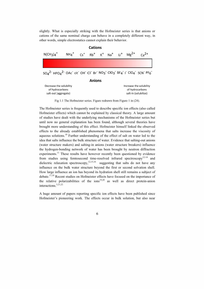
The first scientist who performed a systematic study on specific ions effects was Franz Hofmeister, a professor of pharmacology at the University of Prague. In his work, he observed that different salts, depending on their concentrations, could either increase (salt in) or decrease (salt out) the solubility of proteins in aqueous solutions.9 These findings resulted in a famous classification of ions which is known as the Hofmeister series, as shown in Figure 1.1. Observe that the classification shown in Figure 1.1 is one possible, as there exists several versions for the Hofmeister series where the order of both anions and cations can differ

  

6  

slightly. What is especially striking with the Hofmeister series is that anions or cations of the same nominal charge can behave in a completely different way, in other words, simple electrostatics cannot explain their behavior.

Fig 1.1 The Hofmeister series. Figure redrawn from Figure 1 in (24).

The Hofmeister series is frequently used to describe specific ion effects (also called Hofmeister effects) which cannot be explained by classical theory. A large amount of studies have dealt with the underlying mechanisms of the Hofmeister series but until now no general explanation has been found, although several theories have brought more understanding of this effect. Hofmeister himself linked the observed effects to the already established phenomena that salts increase the viscosity of aqueous solutions.10 Further understanding of the effect of salt on water led to the idea that salts influence the bulk structure of water. Evidence that salting-out anions (water structure makers) and salting-in anions (water structure breakers) influence the hydrogen-bonding network of water has been brought by neutron diffraction experiments.11 These results have however recently been questioned by evidence from studies using femtosecond time-resolved infrared spectroscopy12-14 and dielectric relaxation spectroscopy,12,15,16 suggesting that salts do not have any influence on the bulk water structure beyond the first or second solvation shell. How large influence an ion has beyond its hydration shell still remains a subject of debate.17,18 Recent studies on Hofmeister effects have focused on the importance of the relative polarizabilities of the ions19,20 as well as direct protein-anion interactions.3,21,22

A huge amount of papers reporting specific ion effects have been published since Hofmeister’s pioneering work. The effects occur in bulk solution, but also near

  

7  

surfaces and in the presence of surfactants, polymers and proteins.18 Due to the lack of a complete model including all ionic interactions responsible for the observed effects, one common approach has been to correlate the trends obtained to some common ion property. Polarizability, ionic radius and charge density, viscosity and Gibbs free energy and entropy of hydration are some of the parameters which have been examined.18

The law of matching water affinities23 introduced by Collins in 2004 is an empirical law which contributes to a qualitative explanation for relative ion binding affinities in solution as given by the Hofmeister series. This law stipulates that monovalent ions of opposite charge and with similar hydration energies have matching water affinities. A small ion with high charge density (water structure making or kosmotrope) binds water molecules tightly and will form inner sphere ion pairs with another ion having the same properties. The same goes for large ions with low surface charge density, weakly hydrated with a loosely bound hydration shell (water structure breaking or chaotrope). In the case of two kosmotropes binding to each other, the large electrostatic interaction between the two small ions overcomes the strong water binding to the ions. For two chaotropes, the ions are brought together which allows the released water to form more favorable bonds with other water molecules in the bulk phase.

The law of matching water affinities is a very valuable concept for the classification of ions. It is however important to remember that this empirical law should be taken more as a rule of thumb since the theoretical explanation provided is based on many simplifications.18,24

1.1.4 Metal coordination complexes

In the context of metal coordination chemistry, a complex refers to a central metal atom surrounded by a set of ligands. As previously mentioned, coordination complexes are distinct from ion pairs, even if they can also involve only one cation and one anion. Coordination complexes are formed as a result of the interaction of a Lewis base ligand which donates electrons (donor), used in bond formation, to a central metal atom or ion which acts as a Lewis acid (acceptor). A coordinative covalent bond is formed as a result of this interaction. Ligands may be simple ions, small molecules such as H2O or NH3 or even larger molecules and macromolecules such as proteins. They form the primary coordination sphere of the complex and their number is called the coordination number of the central atom. Three factors govern the coordination number of a complex25

  

8  

The size of the central atom or ion.

The steric interactions between the ligands.

Electronic interactions between the central atom or ion and the ligands. There is also an electrostatic component when the ligand and central metal atom are charged.

When the ligand binds to the metal ion through a single point of attachment, it is said to be unidentate. When two donor atoms from the same ligand bind to the metal, the ligand is said to be bidentate.

The geometrical structure of a metal coordination complex can be studied by X-ray diffraction if single crystals can be grown. NMR can provide information about the structure of complexes in aqueous solutions provided that the lifetime of the complex is sufficiently long. For very short-lived complexes, vibrational and electronic spectroscopy can be used.

Metal coordination complexes are extremely important in biological processes. Examples include chlorophyll, cobalamins (vitamin B12) and the heme complex of hemoglobin which all contain a tetrapyrrole group bound to a metal. Many enzymatic reactions involving nucleotides require the presence of a metal ion. This thesis work has focused on the uranyl ion UO2

2+ and its ability to form complexes with nucleotides. The uranyl ion, in which uranium has an oxidation state of +6, has two relatively inert oxygen atoms.26 The exchangeable ligands are all located in a plane perpendicular to the linear UO2

2+ unit. An example of a complex formed by the uranyl ion with 5 ligands in this plane is [UO2(OH2)5]

2+ which displays a pentagonal bipyramid structure.26

1.1.5 The transport properties of ions in solution

The association state and solvation state, as discussed in previous sections, are intrinsic properties of ions which have an effect on their transport properties in solution. Battery electrolytes such as the ones used in Li ion batteries are often classified according to their transport number (also called transference number). The transport number is defined as the fraction of the current carried by one ionic species in solution. The transport number is a concentration-dependent property and the motion of ions in a Li ion battery under load is due to two driving forces, concentration and potential gradients. Due to the potential gradient in a Li ion battery, ions move through a physical process called migration, the motion of charged particles in an electrical field. The same type of motion occurs in

  

9  

electrophoresis (see Section 1.2.1). Li+ cations move to the negative electrode whereas the anions move to the positive electrode. As the anions are not participating in any reaction, they will accumulate at the positive electrode, giving rise to a concentration gradient over the electrolyte called the diffusion potential. Diffusion (see Section 2.2) will seek to even out the concentration difference present as the anions diffuse to the opposite electrode, bringing the Li+ cations along (due to the electroneutrality criterion). The diffusion potential continues to increase until the diffusion flux is the same as the migration flux of the anions, the magnitude of the fluxes being dependent on the friction forces experienced by the ions.27 In an electrolyte where the anions are moving very slowly, a small concentration difference is created whereas a large concentration difference arises if the anions experience less friction, i.e. move faster, than the Li+ ions.27

 

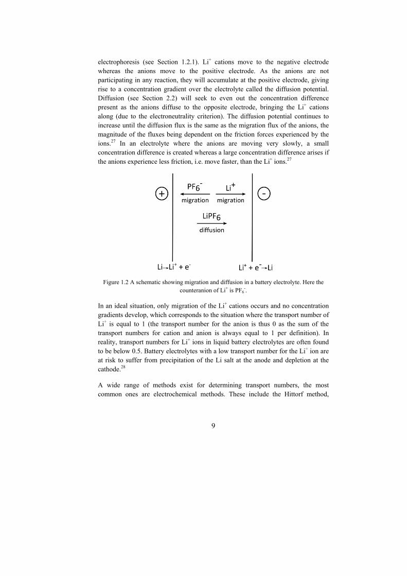
Figure 1.2 A schematic showing migration and diffusion in a battery electrolyte. Here the counteranion of Li+ is PF6

-.

In an ideal situation, only migration of the Li+ cations occurs and no concentration gradients develop, which corresponds to the situation where the transport number of Li+ is equal to 1 (the transport number for the anion is thus 0 as the sum of the transport numbers for cation and anion is always equal to 1 per definition). In reality, transport numbers for Li+ ions in liquid battery electrolytes are often found to be below 0.5. Battery electrolytes with a low transport number for the Li+ ion are at risk to suffer from precipitation of the Li salt at the anode and depletion at the cathode.28

A wide range of methods exist for determining transport numbers, the most common ones are electrochemical methods. These include the Hittorf method,

  

10  

potentiostatic polarization, concentration cells, galvanostatic polarization and electrochemical impedance spectroscopy.27 As is shown here, diffusion NMR and eNMR (see Sections 2.2 and 2.3) can also determine transport numbers (see Paper I). eNMR provides a direct measurement of charge transport through the ionic mobilities. Diffusion coefficients, when measured far from infinite dilution often contain contribution from ion pairs. This parameter also provides information about the solvation of the ions in the electrolyte. It is thus interesting to measure the transport number with several different methods in order to gain a better understanding of the studied electrolyte.

1.2 Methods used to characterize the state of ions in solution

1.2.1 Electrophoresis

When mentioning electrophoresis, a technique used for separating proteins comes to one’s mind. In fact, there exists a wide variety of electrophoretic separation methods that can be applied to a diverse range of materials. Electrophoresis can be done in capillaries, thin-layer plates, films and gels and its purpose can be either to separate compounds from each other but can also be analytical (as in capillary electrophoresis). The technique is also associated to a Nobel Prize in 1948, awarded to Arne Tiselius for the electrophoretic separation using the moving boundary technique.

The principle of electrophoresis is simple. A charged particle of charge ze experiences a force F due to the electric field E applied between two electrodes. Here, z is the effective charge, which differs from the nominal charge denoted by znom. The difference between the nominal and effective charge of a species can be attributed to the relaxation effect and electrophoretic effect (see Section 1.2.2) but also to ion association. The electric field can be expressed as E = U/L where U is the potential difference between the electrodes and L the distance between electrodes. The force F is given by the following relation:

zeUF

L (1.4)

This force leads to acceleration of charged particles. A constant velocity v is rapidly (within typically nanoseconds) obtained when the force due to the electric field becomes balanced by the frictional force. The frictional force is defined as

  

11  

frictionF fv (1.5)

where f is the friction coefficient. The resulting drift velocity is then given as

zeEv

f (1.6)

The velocity v is conventionally expressed as being dependent on the

electrophoretic mobility of the charged particle and the applied electric field E

v E (1.7)

In order to understand the factors governing the motion of the particles in an electric field, the concept of the double-layer that develops in the vicinity of the charged particle (or charged surface) has to be introduced. This double-layer can be described by the concept of the diffuse layer, introduced by Gouy and Chapman. In this layer, both positive and negative ions are present (with an excess of ions with charge opposite to that of the surface), distributed due to thermal motion and due to the effect of surface charge density. The slipping plane defines the distance from the surface at which the fluid can be considered as mobile and the electric potential

at this plane is called the -potential.

Another important concept to be defined is the Debye length which describes how far the double-layer extends into the bulk solution. In other words, a measure of the thickness of the double-layer can be given as

1 0

2

, 0

R B

nom i i

k T

z e C

(1.8)

where znom,i is the nominal charge of the ion and Ci0 is the volume concentration of ions (in some other equivalent expressions Ci0 is replaced by the number density denoted by the symbol n). For a 1-1 symmetrical electrolyte, Eq. (1.8) simplifies to

1 022

R B

A

k T

N e

(1.9)

where NA is the Avogadro number and is the ionic strength (in units of mole m-3).

  

12  

The product of the inverse Debye length times the particle radius, a, is an

important variable which can be used to relate the electrophoretic mobility to the

-potential. The electrophoretic mobility is dependent on how the electric field affects the charged particle and several regimes can be identified depending on the thickness of the double-layer and the size of the particle.

There are two limiting cases which can be treated quite simply. The first case is

when the Debye length is infinitely large and a << 1 (low ionic strength). For such dilute solutions, the force on the particle due to the applied electric field is balanced by the frictional force, as previously described by the use of Eq. (1.5). Combining Eqs. (1.6) and (1.7), the electrophoretic mobility in this limit, µ0, is obtained as

0 ze

f (1.10)

The friction coefficient is given by Stokes law

6f a (1.11)

valid for a sphere with a hydrodynamic radius a in a medium of viscosity and µ0 can thus be expressed as

0

6

ze

a

(1.12)

Eq. (1.12) is central in this thesis work as it has been used in Papers III and V-VII in combination with the Stokes-Einstein equation that gives the diffusion coefficient D as

6Bk T

Da

(1.13)

yielding an expression for the effective charge through the relation known as the Nernst-Einstein equation

0Bk T

zeD

(1.14)

  

13  

Eq. (1.12) can also be expressed in another form by equating the -potential with

the simple surface potential of a sphere given by 04 R

ze

a yielding

0 02

3R

(1.15)

the so-called Hückel equation.

The second case is valid for a small Debye length and a >> 1 (large ionic strength). In this limit, one obtains the so-called Smoluchowski equation29

4 (1 )

ze

a a

(1.16)

0 R

(1.17)

The mobility given by the Schmoluchowski equation is larger than the mobility given by the Hückel equation by a factor 3/2. This can be explained by the distortion of the electric field in the vicinity of the particle and how it affects the ions in the diffuse layer for the two cases described above. For a small Debye length, most electrolyte ions in the double-layer experience a distorted field whereas most electrolyte ions experience an undistorted field for a large Debye length. The electrophoretic effect (see Section 1.2.2), caused by the motion of the ions in the diffuse layer under the applied electric field (in a direction opposite to that of the particle), will thus be less significant for a small Debye length, which explains why the particle will have a higher mobility. 30

In the intermediate case of a ≈ 1, the electrophoretic mobility can be described by

02( )

3R f a

(1.18)

where f(a) is Henry’s function, a function varying, for spherical particles, between

1 (at low a) and 1.5 (at high a).

  

14  

It should be mentioned that none of the relations above take the relaxation effect (see Section 1.2.2) into account. The relaxation effect refers to the distortion of the counterionic cloud (the diffuse layer) due to the applied electric field. This effect is not important for the two cases described above whereas it should be considered for

the intermediate region and especially for high -potentials. The correct expression for the electrophoretic mobility then requires the use of a correction function that is

not only dependent on a but also on . For a numerical treatment which takes the

relaxation effect into account, the reader is advised to consult the papers by Wiersema et al31 and O’Brien and White.32

Another transport mechanism, which should be discussed when describing electrophoresis is electroosmosis. As for electrophoresis, electroosmosis or electroosmotic flow is closely related to the appearance of a double-layer. Electroosmosis arises because of a charged surface, as for example that of a glass capillary where the walls have a negative charge at close to neutral pH due to the presence of deprotonated silanol groups (-Si-O-), being present on the glass surface. Thus, a double-layer with a high concentration of ions forms in the vicinity of the glass wall. When applying an electric field parallel to the glass surface, the

counterions beyond the slipping plane (where the potential is described by the -potential) will start to move and drag the solvent molecules along. Due to viscous coupling to the rest of the liquid body, one obtains a bulk flow of the liquid.

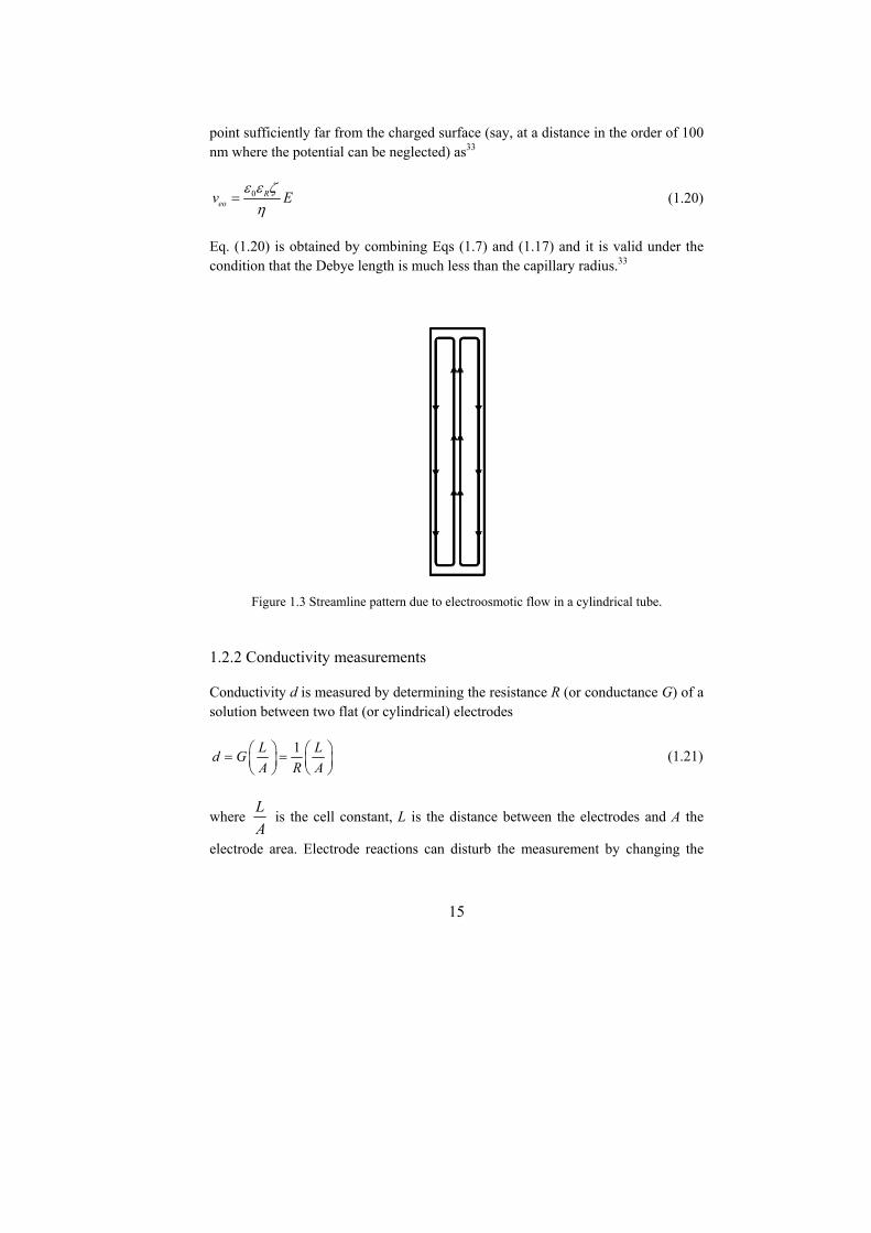
Electroosmotic flow (often abbreviated EOF) can be an advantage as it can move fluids by the action of an electric field. In capillary electrophoresis, it is electroosmotic flow that is used to pull ions (irrespective of their charge) through a long and thin capillary. Electroosmotic flow can also be used in microfluidic devices. In the case of a stagnant liquid column (as for the eNMR measurements described in this thesis work), there will be a counter flow in the middle of the tube leading to a zero net flow. A schematic representation of the streamline pattern in a cylindrical tube is shown in Figure 1.3.

For a cylindrical tube, a velocity distribution develops as33

2

2

2( ) 1eo

tube

rv r v

a

(1.19)

where r is the distance from the centre of the tube, atube the tube radius and veo the slip velocity associated with the electroosmotic surface drag, the latter defined at a

  

15  

point sufficiently far from the charged surface (say, at a distance in the order of 100 nm where the potential can be neglected) as33

0 Reov E

(1.20)

Eq. (1.20) is obtained by combining Eqs (1.7) and (1.17) and it is valid under the condition that the Debye length is much less than the capillary radius.33

Figure 1.3 Streamline pattern due to electroosmotic flow in a cylindrical tube.

1.2.2 Conductivity measurements

Conductivity d is measured by determining the resistance R (or conductance G) of a solution between two flat (or cylindrical) electrodes

1L Ld G

A R A

(1.21)

where L

A is the cell constant, L is the distance between the electrodes and A the

electrode area. Electrode reactions can disturb the measurement by changing the

  

16  

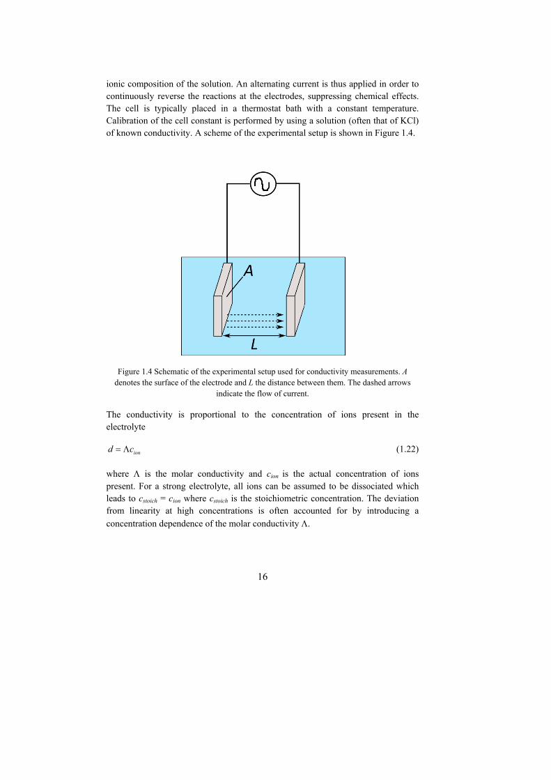
ionic composition of the solution. An alternating current is thus applied in order to continuously reverse the reactions at the electrodes, suppressing chemical effects. The cell is typically placed in a thermostat bath with a constant temperature. Calibration of the cell constant is performed by using a solution (often that of KCl) of known conductivity. A scheme of the experimental setup is shown in Figure 1.4.

Figure 1.4 Schematic of the experimental setup used for conductivity measurements. A denotes the surface of the electrode and L the distance between them. The dashed arrows

indicate the flow of current.

The conductivity is proportional to the concentration of ions present in the electrolyte

iond c (1.22)

where is the molar conductivity and cion is the actual concentration of ions present. For a strong electrolyte, all ions can be assumed to be dissociated which leads to cstoich = cion where cstoich is the stoichiometric concentration. The deviation from linearity at high concentrations is often accounted for by introducing a

concentration dependence of the molar conductivity .

  

17  

For weak electrolytes

ion stoichc c (1.23)

where describes the fraction of ionized species. It is important to note that changes over the concentration range studied. As cstoich approaches 0, the fraction of ionized species will increase dramatically, leading to a strong increase of the molar

conductivity .34 The value that approaches at infinite dilution is called the

limiting molar conductivity .

Electrolyte conduction is often interpreted in terms of the Debye-Hückel model. This model was originally developed to predict the activity coefficients of ions in dilute solutions. In this model, the ions are considered as dimensionless point charges with the only interaction between them being the electrostatic one. The Debye-Hückel model35 was modified by Onsager in 192736 to account for the relaxation and electrophoretic effects pertaining to the concept of an ionic atmosphere.

When an ion moves under an applied electric field, it must build up its ionic atmosphere at each step in the movement. As this process requires some time, the ionic atmosphere will be displaced with respect to the moving ion leading to an asymmetry. This effect is called the relaxation effect. There are two processes responsible for this effect:

The diffusion of ions in the solution which occurs independently from the applied electric field.

When a cation moves towards the negative electrode, it will leave an excess of negative charge behind it (due to the anions moving in opposite direction) and a deficit of negative charge in front. This effect will slow down both anions and cations moving under the electric field as if the asymmetric ionic atmosphere were to pull the ion back.34 The ionic conductivity is therefore reduced.

The so-called electrophoretic effect (sometimes also called electrophoretic retardation effect) arises due to the solvent. When a cation moves under the applied electric field, it carries solvent molecules with it. When this cation meets an anion travelling in the opposite direction, it will be slowed down by the solvent dragged by the anion. This effect also gives rise to conductivity lower than that expected

without an ionic atmosphere.

  

18  

At infinite dilution, the relaxation and electrophoretic effects can be neglected as the central ion is not affected by the presence of other ions. The mobility of an ion

at infinite dilution, is then given by Eq. (1.12) using znom instead of z (effective

charge). At finite concentrations, the mobility is obtained by substracting from the contributions from both the electrophoretic and relaxation effects yielding

3 3

02

0

1

6 144 1 1/ 2nom nom

R B

z e z e

a k T

(1.24)

Eq. (1.24) is equivalent to Eq. (3) in Paper VII and is known as the Debye-Hückel-Onsager limiting law36 often written as

0actualP c (1.25)

where 0P w x with w being a constant dependent on temperature, relative

permittivity and viscosity, and taking account of electrophoresis and x is depending on temperature, relative permittivity and taking account of relaxation.

It is important to point out that this relation holds for a 1-1 symmetrical electrolyte with an ionic strength lower than 1 10-3 mol dm-3. Under those conditions, the actual concentration of free ions can be assumed to be equal to the stoichiometric concentration. Ion pairing, which the theory does not account for, is neglected at this low concentration.

The Debye-Hückel-Onsager model was further developed leading to the Fuoss-Onsager conductance equation in 1957.37 This model considered the relaxation and electrophoretic effects to be dependent on each other (cross terms were included) and also incorporated the effect of ion pairing. One of the drawbacks with this model is that it is only valid at concentrations up to approximately 10 mM for a 1-1

salt in water (or a values up to 0.3, see Section 1.2.1).37 This restriction stemmed from numerical limitations when evaluating the complex mathematical expressions involved.38 A linearized approximation was therefore adopted at the cost of the range of applicability. Unfortunately, it was sometimes used outside its range of validity.38

To date, one of the most used models for analyzing conductivity data is based on the Fuoss-Hsia equation.38 This model has, for example, been used by Barthel and coauthors to study the association of 1-1 electrolytes in various solvents.39-41

  

19  

Finally, it is important to remember that all models describing conductivity are based on approximations and are limited to rather dilute solutions.1

1.2.3 Dielectric relaxation spectroscopy

Dielectric relaxation spectroscopy (DRS) provides the frequency dependent electric permittivity of a sample in an electromagnetic field, over the broad frequency range of 0.01-1000 GHz. As DRS is able to detect species which have a dipole moment, it can thus distinguish between ion pairs (which have a dipole moment) and free ions (which usually do not have a dipole moment). Moreover, the amplitude of the DRS response is proportional to the square of the dipole moment.1 This allows DRS to be sensitive to very weak association1 but can also provide information about the distance between the ions in an ion pair. DRS is sensitive to the various types of ion pairs in the order 2SIP > SIP > CIP.1

An important disadvantage of DRS is that there is no single apparatus that covers the wide frequency range needed. This requires the DRS spectroscopist to combine different instrumentations which often makes the measurement complex and time-consuming. Data interpretation is not trivial either as the obtained spectra are often dominated by the solvent response. This makes proper decomposition into components more difficult and the ion pair contribution harder to retrieve.1 Moreover, the obtained data need to be fitted using a model describing the relaxation processes present in the sample and the number of relaxation processes is not always easy to estimate.1

1.2.4 Spectroscopic methods

Spectroscopic techniques such as NMR, IR, Raman and UV/vis are powerful techniques which can give spectral features which can provide information about ion association. Except for NMR, the details of these techniques will not be presented here. The principle used in the listed techniques is to monitor a change in the obtained spectrum which can then be related to, typically, contact ion pairs. For non-contact ion pairs where the ions are separated by solvent molecules, obtaining reliable data is not straightforward.42

1.2.5 Calorimetric titration

Calorimetric titration is a technique which can be used to study the association of ions to a ligand. It is based on the principle that, when binding occurs, an enthalpy change also takes place. A ligand solution is added continuously to a salt solution in

  

20  

a reaction vessel while temperature changes in the reaction vessel are monitored (in practice the temperature difference between the reaction vessel and a reference cell is recorded). The measured heat transfer at any time during the titration can be related to the amount of products formed due to the interaction between ion and ligand taking place in the vessel and the corresponding binding enthalpies. The binding constant, binding enthalpy and stoichiometry of binding can be estimated by formulating a binding model for the specific interaction taking place and fitting the measured heat transfer to this model.43

An advantage of the technique is that it can be used to study a broad range of processes (since it can be applied to any process involving a heat change). One disadvantage is that it gives no structural information related to the interaction taking place.

1.2.6 Molecular dynamics

Molecular dynamics (MD) simulations have recently become important in describing ion association and studying Hofmeister phenomena (see Section 1.1.3). In MD, successive configurations of the system are generated by integrating Newton’s second law of motion upon the influence of set intermolecular and interatomic potentials (force field). The result is a trajectory that specifies how the positions and velocities of the particles in the system vary with time.44 As MD has limitations both in the size- (number of atoms in the computational cell) and time-domains, it is neither all systems nor all processes that can be studied with this method. The choice of an appropriate force field is important for an accurate result as the result of the simulation strongly depends on it. Moreover, force fields are necessarily approximative.

Molecular dynamics can calculate radial distribution functions (RDF), whose integrals provide information about the number of counterions present within a given distance from the investigated ion. Thus, information about ion pairing and types of ion pairs present can be obtained. This approach has recently been used to study ion pairing between halides and ammonium-containing cations in water,45 selective binding of ions to macromolecules46 and affinity of different anions for either sodium or potassium cations.47 In the last mentioned reference, ab initio calculations were also used in order to compute the free energy change upon replacing one cation with another in the ion pair.

  

21  

2.Experimental

NMR spectroscopy is a powerful and versatile analytical technique. Organic chemists use it to investigate molecular structures with applications in the drug discovery process. Biochemists use it for structure determination of proteins. NMR is also present in the medical field, through its sister technique MRI (Magnetic Resonance Imaging) which allows to image parts of the human body and diagnose diseases such as cancer. In addition, NMR can also answer many important and fundamental questions concerning the behavior of molecules in solutions such as how are they moving and how do they interact with each other.

2.1 Principles of NMR

There are many atomic nuclei which can be observed in NMR, but not all of them. To be NMR-active, nuclei need to have an intrinsic angular and magnetic moment called spin. Some nuclei like 12C which have a spin quantum number I = 0 do not interact with magnetic fields. The component of the angular momentum I along any direction is quantized as

, ,x y zI m (2.1)

where m is the magnetic quantum number that can take 2I+1 values in integer steps

between +I and –I and is the reduced Planck constant . For a proton 1H, I = ½ and the angular momentum will have two states limited to directions Ix,y,z = ± ½. Henceforth, we limit our discussion to nuclei with I = ½. The magnetic moment µ of a nucleus is connected to the spin angular momentum I

μ I (2.2)

where is a proportionality constant known as the gyromagnetic ratio, a property specific for each nucleus. The magnetic moment of a nucleus is thus parallel (or

antiparallel for nuclei with a negative to the spin angular momentum.

In the absence of a magnetic field, the two orientations of the angular momentum Ix,y,z = ± ½ have the same energy. When placing a sample with I = ½ nuclei in a magnetic field B0 along the z-direction (such as in a magnet that belongs to an NMR

spectrometer), the energy E of a magnetic moment µz in the field B0 becomes

0zE B (2.3)

  

22  

Using Eqs (2.1) and (2.2) to rewrite Eq. (2.3) yields

0E m B (2.4)

As m = ± ½, the energy difference E between the two quantized energy states is thus

0E B (2.5)

The spins populate these two energy levels according to the Boltzmann distribution and there is a slight preference for the spins to be in the lower energy level, which,

for positive corresponds to the spins aligned parallel with the field B0 (in a 400 MHz spectrometer at a temperature of 300 K, the ratio of populations of the two levels is 0.9999448). There is thus a small net equilibrium magnetization in the sample along the direction of the magnetic field B0. This equilibrium magnetization forms with a finite buildup time called longitudinal relaxation time, a concept which will be explained later. Once the equilibrium magnetization, often depicted by a magnetization vector M, is formed, it will retain in size and direction.49

NMR spectroscopy relies on the use of radiofrequency (rf) pulses which can be seen as oscillating magnetic fields, to uniformly excite the net magnetization out of its equilibrium state. Rf pulses are characterized by their flip angle and power level (strength). When an rf pulse is applied, the net magnetization vector M, is tipped

away from the z-axis by an angle which is dependent on the length and strength of the pulse. This occurs only if the resonance condition

0E (2.6)

is fulfilled, where

0 0γB (2.7)

is the Larmor frequency.

In this new non-equilibrium state, the nuclear magnetization of the sample starts to rotate around the direction of the magnetic field B0 in a motion called precession,

with a frequency 0.

  

23  

When an rf pulse with an angle of 90° is applied, the magnetization vector M, initially aligned along the field in direction z, is tilted into the xy-plane, also called the transverse plane. The phase of the pulse describes along which direction the applied rf field is aligned, commonly along any of the four cardinal directions x, y, -x and -y. An rf pulse of 90°x tilts the magnetization by a 90° angle around the x-axis and the magnetization vector M becomes aligned along the –y axis. To exemplify this formalism, it is used in Figure 2.1 whereas phase is omitted in the other figures of this chapter.

The precessing magnetization induces a voltage in a suitably placed receiver coil, giving rise to the time-domain signal called free induction decay (FID). The FID is then Fourier transformed and an NMR spectrum with intensity as a function of frequency is retrieved.

All nuclear spins of one sample are uniformly excited when having applied a sufficiently strong rf pulse. They do not, however, precess with exactly the same resonance frequency. This is because the field actually experienced by each nucleus differs slightly from the external field B0. The motion of electrons in nearby orbitals generates additional small fields which can either augment or oppose B0. The resonance condition then becomes

0 (1E σ) (2.8)

where is called the shielding or screening constant. In practice, is not used in evaluating the spectra. Instead, the chemical shift is defined in terms of the difference in shielding between the nucleus of interest and a reference nucleus.

Nuclear magnetization that has been excited by an rf pulse eventually returns to its equilibrium state. There are two relaxation processes involved, the longitudinal relaxation (which occurs with a time constant T1) and the transverse relaxation (with time constant T2). Longitudinal relaxation concerns the return of spin populations back to their thermal equilibrium value. Transverse relaxation refers to the decay of the precessing magnetization in the transverse plane. Relaxation processes are caused by fluctuations in spin interactions that arise due to molecular motions. There are several relaxation mechanisms that may also interact with each other in a complex way. Examples of relaxation mechanisms include the dipole-dipole interaction, quadrupole interaction and the paramagnetic interaction. Relaxation parameters can provide information about molecular association as well as molecular dynamics.

  

24  

Figure 2.1 displays one of the most known pulse-sequences used in NMR, the spin-echo. In this experiment, a 90°

x pulse flips the magnetization into the xy-plane

where the magnetization starts to precess. Due to the distribution of resonance frequencies present, the spins (described by their individual magnetization vectors) precess with slightly different frequencies. Some spins are faster and some slower,

allowing the magnetization to fan out. After a duration of , a 180°y pulse is applied.

The 180° pulse inverts all the magnetization vectors in the xy-plane and these will end up in mirror image positions with respect to the yz-plane.49 The spins that are

slow are now leading ahead and at the duration 2, all the magnetization vectors will become aligned along the -y-axis. This process is called refocusing and the magnetization can be described as coherent when all magnetization vectors align. To fully describe this experiment, transverse relaxation must also be taken into account leading to the refocused magnetization to decay at a rate T2

-1. This effect is not refocused by the 180°

y pulse and will lead to a decrease of the echo amplitude.

Figure 2.1 Scheme of a spin-echo pulse-sequence.

2.2 Diffusion NMR

Self-diffusion is displacement by the random thermal motion (Brownian motion) of molecules. It is characterized by a diffusion coefficient with units of m2s-1 that is the quantity assessed by diffusion NMR experiments. It is important not to confuse self-diffusion with mutual diffusion. Mutual diffusion arises because of a concentration gradient which results in mass fluxes to even out the concentration inhomogeneity.50 The force behind mutual diffusion is the gradient of the chemical potential50. One example is the case of a binary electrolyte where positive ions and negative ions move together at the same speed from regions of higher to lower concentration in order to fulfill the electroneutrality criterion. There will thus be

  

25  

only one mutual diffusion coefficient for the electrolyte. At infinite dilution, the mutual diffusion coefficient approaches the self-diffusion coefficient.

The self-diffusion coefficient is an immensely valuable parameter as it provides information concerning the diffusing entity and its surroundings. How large is the molecule that is diffusing, is it associated to any other compound, how does the geometry of the surrounding medium look like? These are a few (of many) questions that diffusion experiments could help to answer. Information about the size of the diffusing molecule can be accessed through the Stokes-Einstein relation given by Eq. (1.13).

The origin of diffusion NMR experiments dates back to 1950 and to the spin-echo experiment discovered by Hahn. The first diffusion experiments were performed in static inhomogeneous magnetic field until the experimental introduction of Pulsed-Gradient-Spin-Echo NMR (PGSE NMR) in 1965 by Stejskal and Tanner.51

Diffusion experiments are based on the use of magnetic field gradients. When a constant magnetic field gradient is imposed throughout the sample, the magnitude of the magnetic field at any position r is given as

( ) 0B B r g r (2.9)

where g is defined as the spatial derivative of the magnetic field component parallel to B0. In practice, magnetic field components perpendicular to B0 can be neglected assuming the gradient varies along the z-direction.

The Larmor frequency becomes a spatial label50

0z zg z (2.10)

The effect of a gradient pulse has been pictured as twisting the magnetization into a helix52,53 of pitch:

2q g

(2.11)

where is the duration of the gradient pulse and g is the gradient strength (see

Figure 2.2). The helix is a model which describes how the magnetization vectors in the xy-plane vary in the z-direction due to the applied gradient.

  

26  

Figure 2.2 The effect of a gradient pulse along the z-direction on the initially coherent magnetization in the xy-plane in a sample of length L. The magnetization is encoded into a

helix of pitch q. Figure reproduced from Figure 2.1 in (50).  

Observe what happens in the spin-echo based PGSE pulse-sequence shown in Figure 2.3. The first encoding gradient pulse applied after the 90° pulse twists the magnetization into a helix. In the absence of any translational motion, a second identical gradient pulse (in combination with a 180° pulse) applied with appropriate timing can counteract the effect of the first gradient pulse by unwinding the helix in the opposite direction. This second gradient pulse is often denoted as the decoding pulse. The helix rewinds and all magnetization is returned to a coherent state in the xy-plane and is detected as giving a maximum echo signal.

In another scenario, diffusion occurs during the delay and the spins are displaced along the z-axis. Spins that had the same position along the z-axis (at the time of the first gradient pulse) will have moved along the z-axis and thus obtained new (differing) positions as the displacement experienced will be individual for each nuclear spin even though the net displacement of all spins due to diffusion is zero. Thus, at the time of the echo, refocusing is incomplete, leading to a decrease in the magnitude of the net magnetization vector. This occurs because the second gradient pulse cannot counteract the effect of the first gradient pulse as the spins have

changed position and, thereby, resonance frequency during the delay This effect is observed in diffusion NMR experiments where the signal is attenuated as the gradient strength is increased.

  

27  

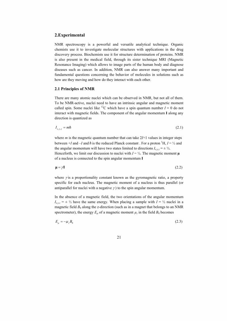
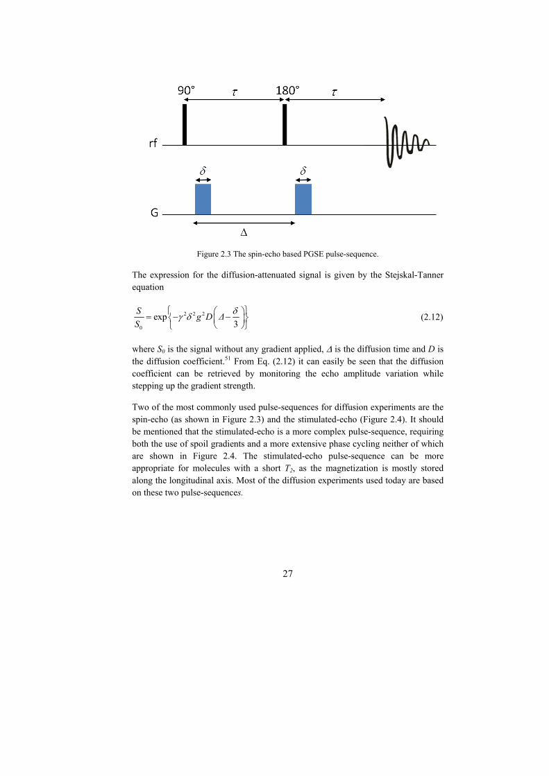
Figure 2.3 The spin-echo based PGSE pulse-sequence.

The expression for the diffusion-attenuated signal is given by the Stejskal-Tanner equation

2 2 2

0

exp3

Sg D Δ

S

(2.12)

where S0 is the signal without any gradient applied, is the diffusion time and D is the diffusion coefficient.51 From Eq. (2.12) it can easily be seen that the diffusion coefficient can be retrieved by monitoring the echo amplitude variation while stepping up the gradient strength.

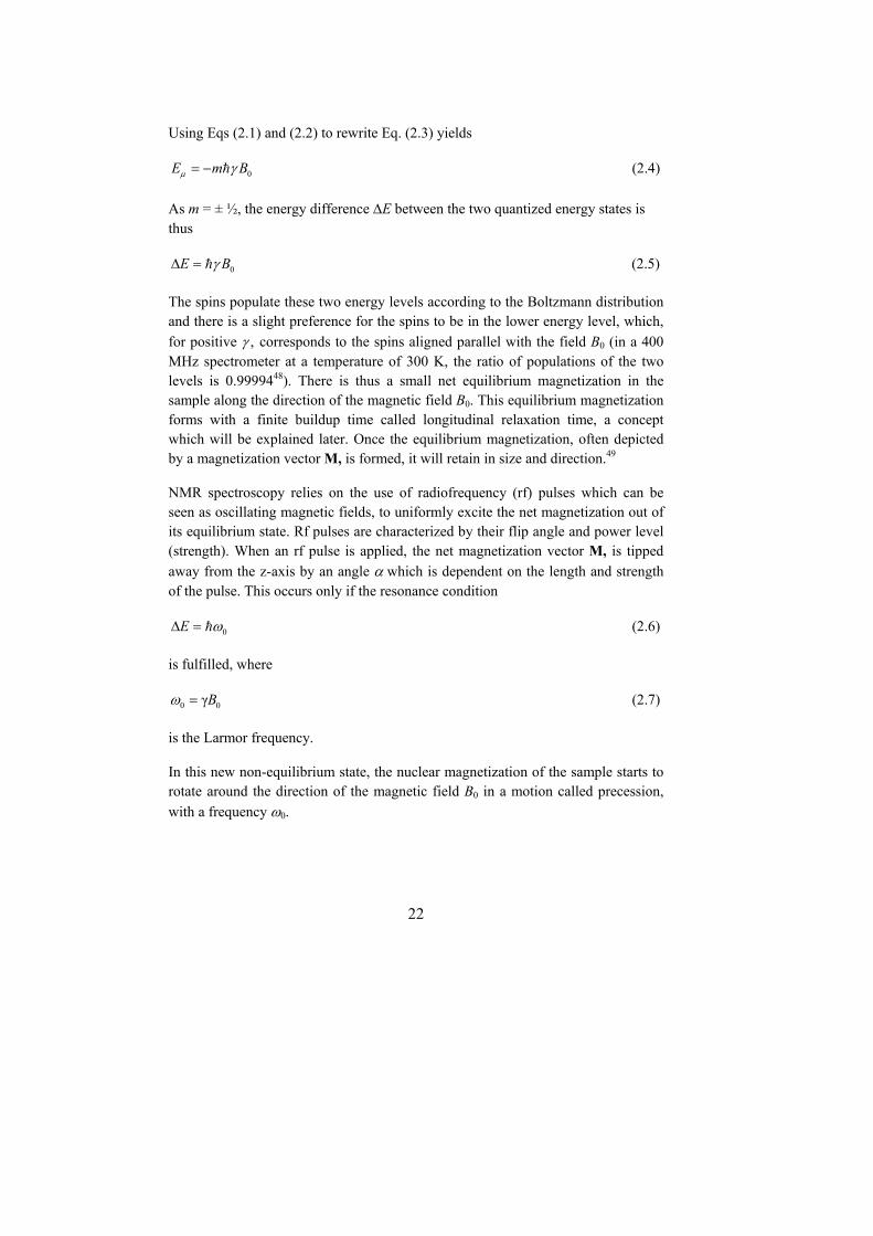
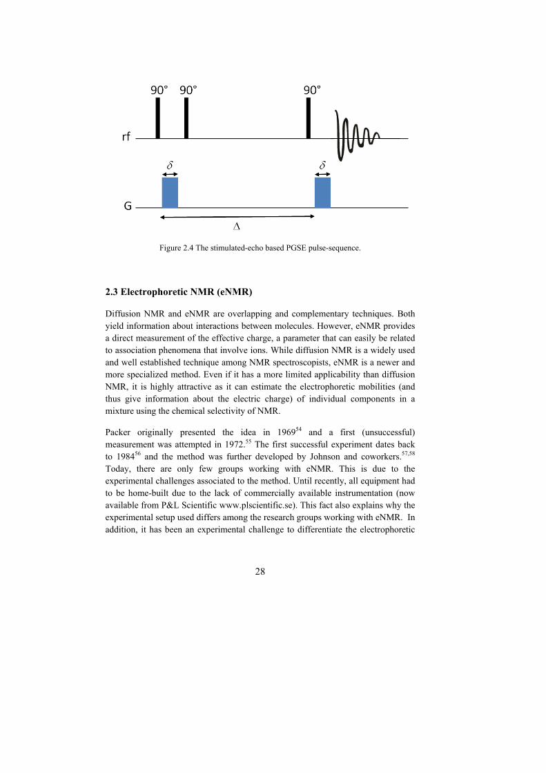
Two of the most commonly used pulse-sequences for diffusion experiments are the spin-echo (as shown in Figure 2.3) and the stimulated-echo (Figure 2.4). It should be mentioned that the stimulated-echo is a more complex pulse-sequence, requiring both the use of spoil gradients and a more extensive phase cycling neither of which are shown in Figure 2.4. The stimulated-echo pulse-sequence can be more appropriate for molecules with a short T2, as the magnetization is mostly stored along the longitudinal axis. Most of the diffusion experiments used today are based on these two pulse-sequences.

  

28  

Figure 2.4 The stimulated-echo based PGSE pulse-sequence.

2.3 Electrophoretic NMR (eNMR)

Diffusion NMR and eNMR are overlapping and complementary techniques. Both yield information about interactions between molecules. However, eNMR provides a direct measurement of the effective charge, a parameter that can easily be related to association phenomena that involve ions. While diffusion NMR is a widely used and well established technique among NMR spectroscopists, eNMR is a newer and more specialized method. Even if it has a more limited applicability than diffusion NMR, it is highly attractive as it can estimate the electrophoretic mobilities (and thus give information about the electric charge) of individual components in a mixture using the chemical selectivity of NMR.

Packer originally presented the idea in 196954  and a first (unsuccessful) measurement was attempted in 1972.55 The first successful experiment dates back to 198456 and the method was further developed by Johnson and coworkers.57,58 Today, there are only few groups working with eNMR. This is due to the experimental challenges associated to the method. Until recently, all equipment had to be home-built due to the lack of commercially available instrumentation (now available from P&L Scientific www.plscientific.se). This fact also explains why the experimental setup used differs among the research groups working with eNMR. In addition, it has been an experimental challenge to differentiate the electrophoretic

  

29  

mobility from the artifactual effects arising during the measurement (see Section 2.3.1). Examples of systems to which eNMR has been applied to include proteins,59 polyelectrolytes,60-62 small ions in solution,63 complexes between cyclodextrins and surfactants64 and complexes between crown ethers and cations.65

The eNMR measurement is essentially the same as a diffusion experiment except that it also employs an electric field applied in the same direction as that of the

gradient during the displacement period. Consider what would happen to the magnetization helix (see Section 2.2) as a result of movement of charged species under an electrical field. As all equally charged molecules move the same distance along the long axis of the helix, the magnitude of the net magnetization vector remains the same. However, the spins are going to be refocused in a direction in the xy-plane that differs from their initial orientation. This difference in the orientation of the spins manifests itself as a phase shift in the obtained NMR spectra.

The acquired phase shift is given by the expression

gvΔ (2.13)

where v is the velocity of the nuclei. Using Eq. (1.7), Eq. (2.13) can be expressed as

g EΔ (2.14)

From Eq. (2.14), it can be seen that the electrophoretic mobility can be estimated

from the linear dependence of the phase shift with increasing electric field strength E. Hence, in contrast to diffusion experiments, it is the electric field (and not the gradient strength) which is stepped up while the gradient strength is kept constant. The expression for the attenuated signal is given by the following expression66

2 2 2

0

exp exp( )3

Sg D Δ i

S

(2.15)

If the diffusion coefficient is determined by a separate experiment, it can easily be seen that the eNMR experiment yields information about the effective charge of the species of interest through the Nernst-Einstein relation in Eq. (1.14).

  

30  

2.3.1 Error sources in eNMR experiments

Thermal convection is an artifact which can arise in standard NMR experiments without any electric field applied. In temperature-regulated experiments, sample heating and cooling is often applied from the bottom part of the NMR tube which leads to temperature gradients in the sample. This is especially a problem when working at temperatures higher than ambient. The severity of convection effects depends on factors such as viscosity of the sample, heater and cooler settings, probe geometry and size of the sample.

As concerning the eNMR sample cell, it is in addition heated up due to the current driven by the electric field applied during the eNMR experiment. The generated heat Q is given by

Q JUt (2.16)

where J is the current, U is the applied potential difference and t is the time. This heating, often called Joule heating, will lead to convective flow. The heat generated in the eNMR experiment will thus be proportional to the current in the sample solution for a given voltage and time. The current is in turn given by the following relation

dAUJ

L (2.17)

where d is the conductivity, A is the cross-sectional area perpendicular to the electric field, U is the applied voltage and L is the length of the eNMR cell (recall that E=U/L). The current generated in the eNMR cell is directly proportional to the conductivity which explains why eNMR as a method performs best in samples with low to moderate conductivity (which translates into samples with low salt concentrations, preferably not exceeding 10 mM).

In theory, convection should not cause any net phase shift as the flow of spins along the direction of the gradient is matched by an identical flow in the opposite direction, yielding a cosine modulation of the signal attenuation50

cosS g Δ E (2.18)

  

31  

In reality, a phase shift due to convective flow is indeed observed; this is due to the rf coil being far from perfect in terms of homogeneity (of the rf field and consequent receptivity). The buildup time for bulk flow due to thermal convection is believed to be in the order of tens of milliseconds or more67 which is in strong contrast to the electrophoretic displacement which occurs on a nanosecond time-scale.

Electroosmotic flow is another type of artifactual flow which can lead to an erroneous electrophoretic mobility. As explained in Section 1.2.1, eletroosmosis is caused by the viscous drag on the solvent due to a layer of ions concentrated along the charged tube walls. In theory, because of the lack of net flow in the NMR tube (see Figure 1.3) it should not cause any net phase shift. In practice, for the same reason as for thermal convection (the inhomogeniety of the rf coil), phase shifts due to electroosmosis can still appear in eNMR experiments. Electroosmosis, as opposed to thermal convection, is dependent on the direction of the applied electric field. The buildup time for electroosmosis is rather long and has been estimated to approximately 100 ms (for aqueous solutions in a tube of 5 mm diameter).33,68,69

In all eNMR experiments, the flows from the two motional artifacts described above will combine. The properties of the solution such as conductivity and viscosity will determine which effect is dominant. The resulting bulk flow can become highly irregular (especially for samples with high conductivity) and cannot be approximated as the sum of the two individual artifactual flow patterns which, indeed, complicates the suppression of these effects.

2.3.2 Error suppression in eNMR experiments

The double stimulated-echo (DSTE) pulse-sequence has been used in several papers in this thesis work (Papers III-VII) and is shown in Figure 2.5. Here, an additional electric field with alternating polarity is applied along the z-axis during the experiment. This has several advantages, one being that the effect of any electrode reaction is reduced. The other advantage is that the phase factors caused by displacements that change direction upon changing the sign of E during the two periods are summed whereas the displacements that do not change direction upon changing the sign of E are, ideally, subtracted from each other.

  

32  

Figure 2.5 The DSTE based pulse-sequence for eNMR.

Indeed, the DSTE pulse-sequence has been shown to suppress some convective effects in diffusion experiments70,71 and also in eNMR experiments.72,73 Whether the DSTE sequence is successful in suppressing electroosmosis depends on the difference in time-scale between this artifactual flow and electrophoresis. For a

typical diffusion time of ms used in several experiments in this thesis work, the effects of electroosmosis are most likely not fully cancelled.

In addition to using a DSTE sequence for eNMR, an NMR signal phase correction procedure is applied67 to further suppress the effect of unwanted convective flows. An uncharged molecule can exhibit a residual phase shift due to convection (this also includes electroosmosis). These effects are corrected for by subtracting the phase shift of the reference from the phase shift of the compound of interest. An example of this procedure is shown in Figure 2.6. It is however not always a trivial task to find an appropriate reference compound. The substance chosen should have the same nucleus as the compound of interest (this is often a problem for eNMR measurements for other nuclei than 1H), must be able to be mixed in at sufficient concentration, and not interact with the target species.

As thermal convection due to Joule heating is not sensitive to the direction of the current, its effect could be expected to be fully cancelled using the DSTE pulse-sequence together with the reference correction. In practice, this is not always the

  

33  

case. The reference correction procedure only compensates in first order for flow artifacts and is not sufficient for highly conductive samples where complex flow patterns can develop due to strong Joule heating in combination with electroosmosis.

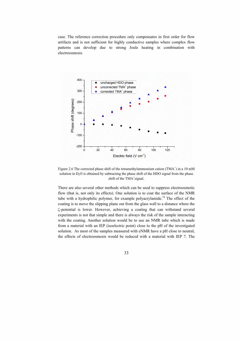
Figure 2.6 The corrected phase shift of the tetramethylammonium cation (TMA+) in a 10 mM solution in D2O is obtained by subtracting the phase shift of the HDO signal from the phase

shift of the TMA+signal.

There are also several other methods which can be used to suppress electroosmotic flow (that is, not only its effects). One solution is to coat the surface of the NMR tube with a hydrophilic polymer, for example polyacrylamide.74 The effect of the coating is to move the slipping plane out from the glass wall to a distance where the

-potential is lower. However, achieving a coating that can withstand several experiments is not that simple and there is always the risk of the sample interacting with the coating. Another solution would be to use an NMR tube which is made from a material with an IEP (isoelectric point) close to the pH of the investigated solution. As most of the samples measured with eNMR have a pH close to neutral, the effects of electroosmosis would be reduced with a material with IEP 7. The

  

34  

currently used borosilicate glass has an acidic IEP. Another alternative, presented in Paper IV (see also Summary of research) uses a pulse-sequence based on a Carr-Purcell-Meiboom-Gill (CPMG) experiment. This pulse-sequence utilizes short electric pulses which primarily reduces the effect of electroosmotic flow because of its rather long buildup time. This method is also successful in suppressing effects of thermal convection and is especially suited for samples of high conductivity.

The electrophoretic sample cell used in this thesis work is based on an NMR tube; it is shown in Figure 2.7. The electrodes are made of palladium wire which has been shown to absorb and store hydrogen to a considerable extent. Bubble formation resulting from H2 generation due to water electrolysis is thus reduced.67 Even though the lower electrode runs across the rf sensitive volume, reasonable peak width (at half height) of around 5 Hz can be achieved for proton spectra in aqueous solutions. The electrode wires are surrounded by glass capillaries which can be sealed at the top and bottom to the electrode. However, care should be taken when using silicon glue or other adhesives as it is difficult to exclude any reaction between the sample and the glue. This is why most experiments in this thesis work were performed without sealed capillaries. Instead, a small amount of soldering wire was melted onto the electrodes, close to the capillary upper end, to prevent the capillaries from changing position along the electrode wire. After each experiment, the inside of the capillaries was rinsed and dried to prevent any contamination. The distance between electrodes was roughly 3.5 cm and this distance was calibrated using the known mobility of the TMA+ cation in a 10 mM solution of tetramethylammonium bromide (TMABr) in D2O.67

The eNMR cell described here is not the only cell design available. One setup which has been used quite extensively is the U-tube sample cell.72,75,76 Even if it possesses advantages like having the electrodes outside the rf sensitive volume, the filling factor is low and the cell is more sensitive to electroosmosis due to its small inner diameter. Moreover, the sign of the electrophoretic mobility is lost as the direction of ionic velocity are opposite in each tube half. Hence, reference correction as in Figure 2.6 becomes impossible. Using this design requires coating of the tube walls to suppress the effect of electroosmosis.

An improvement to the current 5 mm eNMR cell used here would be to have the electrodes outside the sample volume. However, this modification is not straightforward as it would require the lower electrode to be connected from below and a modification of the NMR probe would become necessary. Another possibility

  

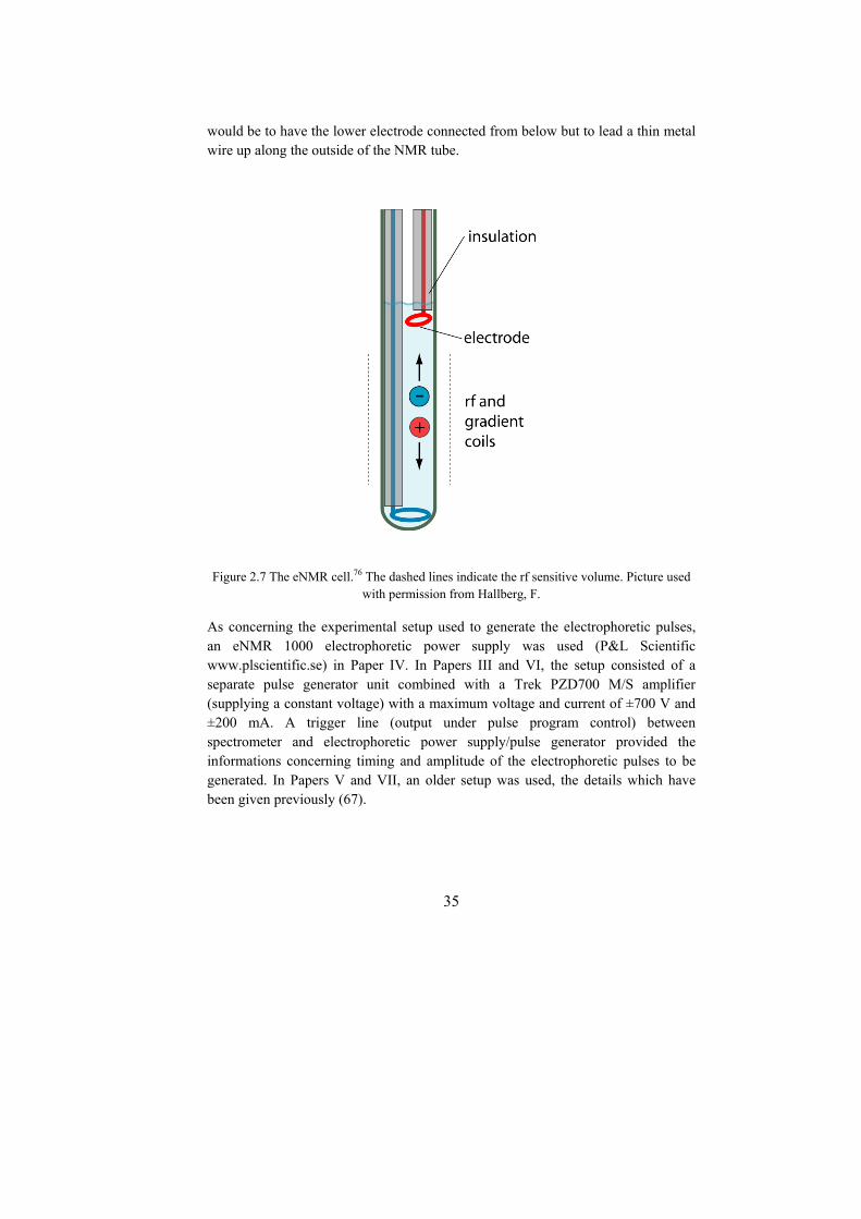
35  

would be to have the lower electrode connected from below but to lead a thin metal wire up along the outside of the NMR tube.

Figure 2.7 The eNMR cell.76 The dashed lines indicate the rf sensitive volume. Picture used with permission from Hallberg, F.

As concerning the experimental setup used to generate the electrophoretic pulses, an eNMR 1000 electrophoretic power supply was used (P&L Scientific www.plscientific.se) in Paper IV. In Papers III and VI, the setup consisted of a separate pulse generator unit combined with a Trek PZD700 M/S amplifier (supplying a constant voltage) with a maximum voltage and current of ±700 V and ±200 mA. A trigger line (output under pulse program control) between spectrometer and electrophoretic power supply/pulse generator provided the informations concerning timing and amplitude of the electrophoretic pulses to be generated. In Papers V and VII, an older setup was used, the details which have been given previously (67).

  

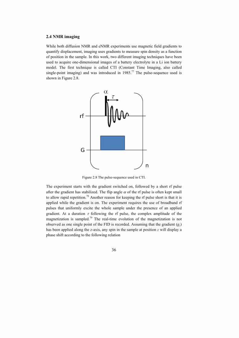
36  

2.4 NMR imaging

While both diffusion NMR and eNMR experiments use magnetic field gradients to quantify displacement, imaging uses gradients to measure spin density as a function of position in the sample. In this work, two different imaging techniques have been used to acquire one-dimensional images of a battery electrolyte in a Li ion battery model. The first technique is called CTI (Constant Time Imaging, also called single-point imaging) and was introduced in 1985.77 The pulse-sequence used is shown in Figure 2.8.

Figure 2.8 The pulse-sequence used in CTI.

The experiment starts with the gradient switched on, followed by a short rf pulse

after the gradient has stabilized. The flip angle of the rf pulse is often kept small to allow rapid repetition.78 Another reason for keeping the rf pulse short is that it is applied while the gradient is on. The experiment requires the use of broadband rf pulses that uniformly excite the whole sample under the presence of an applied

gradient. At a duration following the rf pulse, the complex amplitude of the magnetization is sampled.79 The real-time evolution of the magnetization is not observed as one single point of the FID is recorded. Assuming that the gradient (gz) has been applied along the z-axis, any spin in the sample at position z will display a phase shift according to the following relation

  

37  

zg z (2.19)

As CTI is often the method of choice for species with short T2, the delay is kept

short. Another reason for keeping short is that the magnetization decays rapidly under the applied gradient. The sequence is repeated with the value of gz incremented for each repetition. The increment in gradient strength dgz is given by the relation79

2πzdg

z

(2.20)

where z is the field of view.

The magnetization taken at each gradient step will be the sum of spin phases for all positions along the gradient axis. The sequence is repeated for each gradient step using the increment defined by Eq. (2.20). Thus, in CTI, the spatial information is encoded in the signal phase modulation in reciprocal space S(k), where k is the reciprocal space vector defined as

2

g

k (2.21)

Using the concept of the Fourier transform, the signal S(k) and the spin density

(r)are mutually conjugate

( ) ( ) exp i2 dS k r k r r (2.22)

Eq. (2.22) is central in NMR imaging and explains how the spin density can be retrieved from the obtained signal.

As the real-time evolution of the magnetization is not measured in CTI, the images are free from distortions arising from B0 inhomogeneity and chemical shift.80

Another pulse-sequence which can be used for one-dimensional imaging is based on the spin-echo pulse-sequence (see Figure 2.9) and is called spin-echo imaging. This method, as opposed to CTI, is not based on phase-encoding but on frequency-encoding.

  

38  

Spin-echo imaging is often used in clinical applications where slight modification of the pulse-sequence can provide T1 or T2 weighted images. Spin-echo imaging is a simple and fast method for obtaining one-dimensional profiles of an object. It can however not be used for compounds with a short T2 time. For a comparison on the sensitivity of CTI and spin-echo imaging, the reader is recommended to consult the article by Gravina and Cory.79 In this thesis work, spin-echo imaging was used to obtain one-dimensional profiles of a Li ion battery electrolyte under polarization (see Paper I). The method was chosen over CTI as a better signal-to-noise ratio could be obtained together with the fact that, for that particular sample, the obtained profiles did not suffer significantly from susceptibility effects. One should keep in mind that if, for example, smaller objects were to be studied, approaching the dimensions of real Li ion batteries, CTI would be a more suitable method.

Figure 2.9 The one-dimensional spin-echo imaging pulse-sequence.

  

39  

3. Summary of research

3.1 Methodology

3.1.1 Suppression of artifactual flows in highly conductive samples

One of the challenges with eNMR as a measurement technique is to make it available for all types of samples. This is complicated by the fact that motional artifacts arise due to the application of an electric field during the experiment. The sources are convective flow from Joule heating and electroosmosis, the details of which have been given in Sections 1.2.1 and 2.3.1.

In this thesis work, the majority of eNMR experiments have been performed with the double stimulated-echo (DSTE) pulse-sequence. As explained earlier (see Section 2.3.2), this pulse-sequence compensates rather well for thermal convection in samples with moderate conductivity (≈ 0.1 S m-1) together with the use of a signal phase correction procedure. It is less straightforward to correct for electroosmosis as that is, like electrophoresis, dependent on the direction of the electric field. An additional complication arises for samples with high conductivity where thermal convection and electroosmosis combine which can eventually lead to highly irregular flow patterns.

Paper IV presents the use of the Carr-Purcell-Meiboom-Gill with Electric field Reversal (CPMGER) pulse-sequence as a means to overcome these issues (see Figure 3.1). This pulse-sequence utilizes short electric pulses which primarily reduces the effect of electroosmotic flow because the latter has a rather long buildup time.

The cumulative intensity decrease for the CPMGER experiment is derived as

22

0 03

8 18

2 32

s

CPMGER DSTE

Δg a

nS S n S S

n

(3.1)

where it can be seen that the signal loss is expected to be significantly smaller than for the DSTE experiment (here, n denotes the amount of segments in the pulse- sequence and as is the acceleration). In reality, even if the CPMGER was found to be far superior in reducing phase imperfections, the difference between these two pulse-sequences was not as large as predicted by Eq. (3.1). This was ascribed to

  

40  

increased electroosmotic acceleration due to the fast switching of electric field direction for CPMGER.

Figure 3.1 The CPMGER pulse-sequence (phase cycling omitted here, see details in Paper IV).

CPMGER requires the use of a suitable voltage source which allows for a fast switching of stable bipolar voltage pulses. Since it is a spin-echo method, it is not appropriate for species with a short transverse relaxation time T2.

The performance of the CPMGER was first tested on a sample with low conductivity (uncharged PEO in D2O). No phase shift was observed for either PEO or HDO in D2O and the signal intensity was constant as opposed to DSTE which showed a significant phase shift for both species and a reduced intensity as the electric field was increased. The CPMGER method was further tested on a sample of 10 mM TMABr in D2O with a conductivity of ≈ 0.089 S m-1. For this sample, CPMGER also performed better, reducing the signal loss significantly. As concerning the phase shift of the uncharged reference signal (HDO in D2O), it

decreased as n was increased while was keptconstant. At the lowest accessible

value of /8n of 3.5 ms (see Figure 3.1), the phase correction term amounted to 20 times less than for the DSTE experiment.

Finally, CPMGER experiments were performed on a dissociated salt in D2O, where 19F was the observed nuclei for the anion and 1H the observed nuclei for the cation. This experiment was to exemplify the future use of the pulse-sequence for ionic

  

41  

liquids (where the anion often contains a fluorine atom), systems of high conductivity for which it is desirable to avoid adding a reference molecule even at low concentrations.

3.1.2 Constant-time chemical-shift selective imaging

Two papers in this thesis work have dealt with NMR imaging in a Li ion battery model. Paper I has focused more on the application of this technique while Paper II has dealt with some experimental aspects. Two different NMR imaging techniques have been explored, CTI and spin-echo imaging, the details of which have been given in section 2.4. In Paper II, the focus was on CTI (see Section 2.4). Since in CTI the signal is broadened by gradient, distinction between spin species of different chemical shift is lost. Thus, when applied to an axially symmetric cell with two cylindrical Li metal plates at its opposite ends and with an electrolyte containing Li+ ions held in-between, the 1D 7Li profile obtained (along the vertical axis, or z-axis) reflects Li distribution in both the electrodes and the electrolyte. This can be a problem especially when the aim is to image changes in the electrolyte concentration when the cell is under applied current (see Paper I). In the initial stages of polarization, only small effects at the edges of the electrolyte profile can be observed and the presence of electrodes in the image renders the observation of these effects difficult. Paper II provides a way to modify the original CTI pulse- sequence in order to make it chemically selective. The constant-time chemical-shift selective (CTCSI) imaging pulse-sequence utilizes the fact that a sufficiently long time window is available between the gradient pulses (see Eq.(1) in Paper II). Thus, a chemically selective saturation pulse was applied before the gradient is switched on. In the present system, CTCSI was especially easy to implement due to a large difference of 50 kHz between the resonances for the Li metal and the Li+ ions in the

electrolyte. By applying a pulse of duration of 30 ms with a pulse angle of 220, a profile displaying only the electrodes or only the electrolyte was obtained. These are shown in Figure 3.2 and compared with the profile obtained with a standard CTI experiment.

  

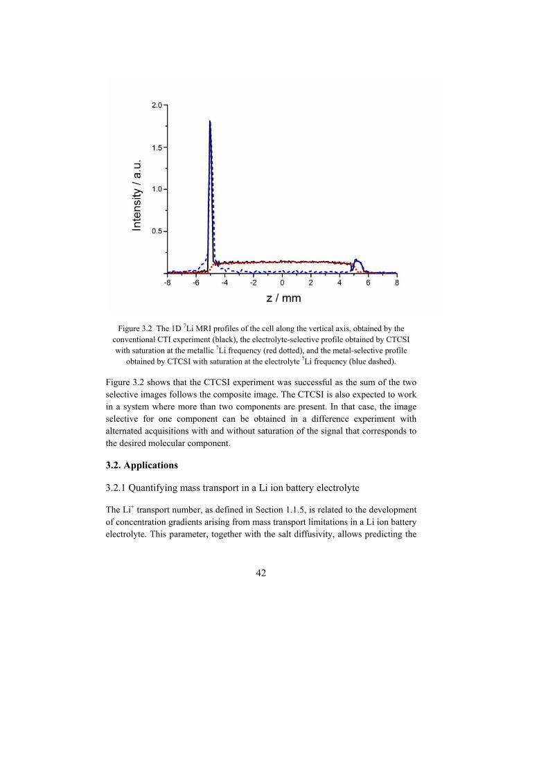
42  

Figure 3.2 The 1D 7Li MRI profiles of the cell along the vertical axis, obtained by the conventional CTI experiment (black), the electrolyte-selective profile obtained by CTCSI with saturation at the metallic 7Li frequency (red dotted), and the metal-selective profile

obtained by CTCSI with saturation at the electrolyte 7Li frequency (blue dashed).

Figure 3.2 shows that the CTCSI experiment was successful as the sum of the two selective images follows the composite image. The CTCSI is also expected to work in a system where more than two components are present. In that case, the image selective for one component can be obtained in a difference experiment with alternated acquisitions with and without saturation of the signal that corresponds to the desired molecular component.

3.2. Applications

3.2.1 Quantifying mass transport in a Li ion battery electrolyte

The Li+ transport number, as defined in Section 1.1.5, is related to the development of concentration gradients arising from mass transport limitations in a Li ion battery electrolyte. This parameter, together with the salt diffusivity, allows predicting the

  

43  

performance of battery electrolytes in terms of mass transport. Observe that the diffusivity mentioned in Paper I is distinct from the self-diffusion coefficient measured by diffusion NMR (see Section 2.2). Here, the salt diffusivity is related to the Maxwell-Stefan diffusion coefficients which describe mutual diffusion in a multicomponent system.

Paper I presents a novel method based on NMR imaging that has been used to characterize the electrolyte of a Li ion battery model under applied current. The development of concentration gradients in the electrolyte was studied by recording (1D) 7Li images of the electrolyte using spin-echo imaging (see Section 2.4) while a constant current was applied. The Li ion battery model studied here consisted of an axially symmetrical cell, with a Li electrolyte (1 M LiPF6 in 1:1 ethylene carbonate (EC)/ diethylene carbonate (DEC) mixed with 15 wt % poly(methyl methacrylate), where the polymer was added to prevent convection) held between two Li metal electrodes connected to external wires for in situ current control. The obtained profiles of the electrolyte are shown in Figure 3.3.

Figure 3.3 1D 7Li NMR images of the Li ion battery model to which a constant current of 30 µA was applied.

Diffusion experiments with variable diffusion time revealed that convection was not significant for the current direction and values applied. An electrochemical model described the local salt concentration in the cell by a partial differential equation

  

44  

with associated boundary conditions. By fitting the solution of this equation to the measured profiles, the transport number for Li+ and salt diffusivity was obtained. Although this electrolyte has not been characterized earlier, the agreement with transport properties for similar systems was good. The transport number for Li+ was also estimated using diffusion NMR, which gave a higher value than the one obtained by in situ 7Li imaging. This was ascribed to the difference in definition of the transport number for these two methods, diffusion NMR taking the contribution from ion pairs into account.

This new method is rather unique as it offers the possibility to directly visualize the concentration gradients developed in a battery electrolyte.7Li NMR imaging can be used to detect, as well as validate, transport parameters obtained with nondirect electrochemical methods which rely on measuring potential and relating it to salt concentration. A future perspective would be to apply this method to Li battery models approaching the dimensions of a real battery. CTI could then become an alternative in order to avoid large susceptibility effects. Changing nucleus of observation from 7Li to 19F would also allow shortening the measurement time and thereby allow visualization of rapid concentration changes.

3.2.2 The protonation state of the ligand in a uranium(VI)-AMP complex by eNMR

In Paper III, the effective charge of the ligand in a metal coordination complex formed between uranyl ions and adenosine monophosphate (AMP) was determined by eNMR measurements. This complex, with a metal to ligand ratio of 3:3, forms in aqueous solution in the alkaline pH range. The aim of the study was to determine whether or not the monodentate 2-OH oxygens of the complex are protonated. Tetrabutylammonium hydroxide (TBAOH) was used to adjust the pD to the range where the complex forms. A separate eNMR experiment with only TBAOH in the same concentration and pD range allowed to determine the effective charge of the TBA+ cation without the complex present. The degree of association of TBA+ to the complex was estimated using a fast exchange model and the nominal charge of the complex could thereafter be calculated. The value of the nominal charge revealed that, at a pD of 11.9, the monodentate 2-OH oxygens were protonated whereas the deprotonation was partial at a pD of 13.

  

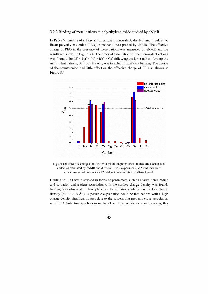
45  

3.2.3 Binding of metal cations to polyethylene oxide studied by eNMR

In Paper V, binding of a large set of cations (monovalent, divalent and trivalent) to linear polyethylene oxide (PEO) in methanol was probed by eNMR. The effective charge of PEO in the presence of these cations was measured by eNMR and the results are shown in Figure 3.4. The order of association for the monovalent cations was found to be Li+ < Na+ < K+ ≈ Rb+ ≈ Cs+ following the ionic radius. Among the multivalent cations, Ba2+ was the only one to exhibit significant binding. The choice of the counteranion had little effect on the effective charge of PEO as shown in Figure 3.4.

Fig 3.4 The effective charge z of PEO with metal ion perchlorate, iodide and acetate salts added, as estimated by eNMR and diffusion NMR experiments at 2 mM monomer

concentration of polymer and 2 mM salt concentration in d4-methanol.

Binding to PEO was discussed in terms of parameters such as charge, ionic radius and solvation and a clear correlation with the surface charge density was found: binding was observed to take place for those cations which have a low charge density (<0.10-0.15 Å-2). A possible explanation could be that cations with a high charge density significantly associate to the solvent that prevents close association with PEO. Solvation numbers in methanol are however rather scarce, making this

  

46  

hypothesis difficult to verify. For Ba2+, the anion was found to associate to the polymer-cation complex (in agreement with an earlier conductometric study81) since extensive ion-pairing was present in the studied solutions.

In the related work of Paper VI, binding of Li+, K+ and Ba2+ to short PEO chains in methanol was studied. Here, the amount of charge bound per monomer unit was significantly higher (by a factor 3-4 for K+) than for the PEO polymer with high molecular weight studied in Paper V. This effect was attributed to a high entropy cost needed for the long polymer chain to rearrange itself in order to optimize the number of ion-dipole interactions. Another interesting observation was that, in the range of PEO units from 8 to 27, the effective charge of PEO increased linearly in the presence of K+ whereas it more or less stayed constant with Ba2+. This finding, together with results from diffusion measurements, relaxation measurements and chemical shift data seem to suggest two distinct binding modes for short PEO chains in the presence of these two cations.

3.2.4 Ion pairing in various solvents studied by eNMR

In Paper VII, the ion pairing behavior of the tetramethylammonium cation (TMA+) in various solvents including D2O, DMSO, acetonitrile, methanol and ethanol was studied by eNMR. The difference between nominal and effective charge, described by the parameter p,

nom effp z z (3.2)

was obtained for TMA+. Using the Debye-Hückel-Onsager limiting law accounting for the relaxation and electrophoretic effects (see Section 1.2.2), a theoretical electrophoretic mobility for TMA+ was predicted and thus a theoretical value of p could be obtained. This limiting law, assumed to be valid at low concentrations, could be applied here as the concentration of TMA salts was 2 mM. The difference in measured p (by eNMR) and calculated p was ascribed to ion pairing as the Debye-Hückel-Onsager limiting law does not take that effect into account. Ion pairing was found to be negligible in D2O, DMSO and methanol whereas it was significant in acetonitrile and ethanol. These findings indicate that the dielectric constant alone is not sufficient to predict the degree of ion pairing in a specific solvent. Other molecular properties/details must be important as well.

  

47  

Conclusions and future work

This thesis work has shown that eNMR in combination with diffusion experiments is a reliable method which allows one to determine the effective charge of a charged species. This parameter can easily be used to quantify ionic association without the use of any advanced models. Here, eNMR was applied to ion pairing, binding of cations to a polymer through the ion-dipole interaction and ligand association to an ion in a metal coordination complex. For the systems studied here, good agreement was found with data obtained by other methods, some of which were presented in this thesis. Moreover, eNMR measurements have the advantage of being fast and relatively easy to process. When the sample studied is a mixture, eNMR can provide information on the association state of all components, provided that the signals do not significantly overlap.

In order to obtain reliable data from eNMR measurements, proper suppression of the effects of artifactual flow is required. For samples of moderate conductivity, this could be achieved by using a sample cell based on a standard NMR tube together with a DSTE pulse-sequence and a reference correction method. This thesis work has presented an alternative pulse-sequence, based on CPMG, which successfully suppresses flow effects and will prove more suitable for samples of high conductivity.

In another experimental setup, 7Li NMR imaging experiments allowed to visualize the concentration gradients developing under applied current in the electrolyte of a Li ion battery model. Transport parameters were obtained by fitting the obtained data to an electrochemical model. Also here, the obtained parameters were in good agreement with parameters obtained by other methods and reported in the literature. Two types of NMR imaging experiments, with slightly different ranges of applicability were implemented, allowing this new in situ imaging method to be flexible in terms of the size of the systems studied.

eNMR is a rather new technique which until now has only been applied to a few types of systems. This is in part due to limitations arising from perturbing artifactual flow. It would be interesting to continue working with CPMGER in highly conductive systems. Initial experiments have been performed in ionic liquids, both with the DSTE and CPMGER pulse-sequences. eNMR could provide here the effective charge of both cation and anion in neat ionic liquids, quantities which seldom have been reported in the literature. Moreover, eNMR has been shown to be a reliable method for studying ion association to other ions and to

  

48  

polymers. There exists a wide variety of other systems which eNMR could be applied to.

As concerning the imaging experiments in batteries, it would be interesting to quantify a commercially available electrolyte and compare the results with data obtained with other methods. This requires the removal of the added polymer which was used to suppress effects from thermal convection. Instead, a column consisting of separators (filters) inserted in the electrolyte, in-between the two metal electrodes, could prevent convection from developing. Another alternative would be to reduce the height of the liquid column, approaching the dimensions of a real Li ion battery. Optimization of 19F imaging experiments could allow for shorter experiments than for 7Li and subsequently for the use of higher currents. Eventually, this method could also be used to study not only the ion transport in the electrolyte, but also chemical processes taking place in a battery.

 

 

 

  

49  

List of abbreviations and symbols

a Particle radius as Acceleration atube Tube radius A Area B0 Static magnetic field B(r) Magnitude of magnetic field at position r c Molar concentration C Volume concentration d Conductivity D Diffusion coefficient e Elementary charge E Electric field

E Energy of a magnetic moment in a magnetic field f Friction coefficient F Force g Magnetic field gradient strength gz z-component of the magnetic field gradient g Magnetic field gradient (vector) G Conductance

Reduced Planck constant I Spin quantum number Ix,y,z component of the spin angular momentum I along any direction I Spin angular momentum vector J Current kB Boltzmann factor k Reciprocal space vector KA Association constant L Length (between electrodes) m Magnetic quantum number M Equilibrium magnetization vector n Number of segments in the CPMGER sequence NA Avogadros number p Difference between nominal charge znom and effective charge zeff

P Variable in the Debye-Hückel-Onsager limiting law Q Heat r Distance from centre of tube

  

50  

r Position (vector) R Resistance S Signal in an NMR experiment S0 Signal in a diffusion NMR/eNMR experiment without any gradient

applied S(k) Signal intensity in reciprocal space t Time T Temperature T1 Time constant for longitudinal relaxation T2 Time constant for transverse relaxation U Potential difference v Velocity w Constant in the Debye-Hückel-Onsager limiting law x Constant in the Debye-Hückel-Onsager limiting law znom Nominal charge z Effective charge  

Greek letters

Flip angle of rf pulse

Fraction of ionized species

Ionic strength

Duration of gradient pulse

Diffusion time

Energy difference

z Field of view

0 Vacuum permittivityR Dielectric constant

Phase shift

Gyromagnetic ratio

Viscosity

Inverse Debye length

Debye length

Bjerrum length

Molar conductivity

Limiting molar conductivity

q Helical pitch length

  

51  

Electrophoretic mobility

z z-component of the magnetic moment

Magnetic moment vector

r Spin density Shielding constant

Duration used in pulse-sequences Larmor frequency

z z-component of the Larmor frequency

Zeta potential

 

 

 

  

52  

Acknowledgements

This thesis is the result of several years of work. Many people have helped me along the way and I would like to thank them: Thank you Prof. Peter Stilbs and Prof. István Furó for accepting me as a PhD student in your department and giving me this great opportunity. Thank you Prof. Peter Stilbs for sharing your knowledge, and for interesting discussions, fast feedback on my manuscripts, and for creating a positive work atmosphere. Thank you Prof. István Furó for your dedication, enthusiasm, and for sharing your knowledge and your great ideas. Also, for leaving me enough freedom in my work and encouraging a passion for research. My coauthors for interesting and fruitful collaborations. I have learned a lot from working with you. Dr. Matilda Klett, I am very happy that I had the chance to work with you and I really enjoyed our collaboration. Prof. Per Claesson for reviewing the thesis and making valuable comments. Lena Skowron, Vera Jovanovic and Dr. Ulla Jacobsson have been very helpful with all administrative matters and questions related to thesis preparation. The Swedish Research Council (VR) and the Knut and Alice Wallenberg Foundation are gratefully acknowledged for financial support. Associate Prof. Sergey Dvinskikh, thank you for all your help with the spectrometers and for your great pedagogical explanations on any question related to NMR. Dr. Pavel Yushmanov for your kind and efficient help with the spectrometers, building (and repairing ) NMR cells for imaging, and helping me with eNMR pulse-sequences. My current colleagues at the division of Applied Physical Chemistry for creating a nice work atmosphere and helping me out in many different ways. Thank you Erik, Fredrik, Ricardo, Yuan, Jing, Boris, Mika, Joakim, Björn and Kristina. I have enjoyed the days in the labs with you and the fun times at our after-works!

  

53  

Also, thank you to my colleagues with whom I have shared the office in the last years. Thank you Yuan, I enjoyed working with you and all our discussions, whether on eNMR or not. Thank you also to Dr. Robert Corkery for many inspiring discussions. Thank you Fredrik for showing me how to do NMR measurements during my first months at Physical Chemistry. Thank you to my former PhD colleagues Carina and Anton for friendship and positive inspiration. Thank you Raquel for the many enjoyable times that we shared while you were visiting our lab during your PhD. Thank you to my former postdoc friends, Michal, Shipra, Guilhem, Camilla and Åsa for support, inspiration, interesting discussions and nice times at dinners and after-works. Åsa, I really enjoyed working with you. Thank you for being a good friend and a source of positive inspiration. Camilla, thank you, too, for being a good friend and a great source of positive inspiration. Dr. Arne Lundin at Biothema AB, Prof. Takashi Kato, Dr. Yuko Kamikawa, and Dr. Sanami Yazaki at the University of Tokyo, Dr. Martin Orbe at GEMS PET Systems/GE Healthcare, and Dr. Irina Velikyan at Uppsala University, for initial inspiration that led me to start out on a PhD. Thank you to my friends, Anna-Karin and Anders, Monica and Markus, Joanna, Mattias, Åsa and Micke, Elin and Shanker. I am very thankful to have you in my life and I so much enjoy the time we spend together. Kerstin and Ken for the many enjoyable times we have spent together and because it always feels good being with you. Helena, for long-lasting friendship and many interesting discussions about life. Sanami, for great friendship even though we live far away from each other. My husband Fredrik’s family for being warm and welcoming and many nice times during birthday celebrations, christmas eve’s and summer holidays in Stallarholmen and in Gotland. My aunt Simone and my uncle Göran for their kindness and warmth and for beautiful summers at Almö during the first years of my PhD.

  

54  

My cousin Marina for always caring about me and for her great generosity. My parents for their endless love and support whatever I undertake here in life. For always being there for me and believing in me. Thank you also for all help with babysitting during work with this thesis. My husband Fredrik for endless love, support, understanding and patience. Because you always listen and for all wise advice on questions related to PhD times. And because I feel happy and balanced being with you. My daughter Isolde for giving a deeper meaning to my life and because you brighten my days with your beautiful smile and a whole lot of “bus”. And because trying to see the world through your eyes is truly enjoyable.

 

 

  

55  

References

1. Marcus, Y.; Hefter, G. Chem. Rev. 2006, 106, 4585-4621. 2. Wachter, W.; Fernandez, S.; Buchner, R.; Hefter, G. J. Phys. Chem.

B 2007, 111, 9010-9017. 3. Zhang, Y. J.; Furyk, S.; Bergbreiter, D. E.; Cremer, P. S. J. Am.

Chem. Soc. 2005, 127, 14505-14510. 4. Tiktopulo, E. I.; Uversky, V. N.; Lushchik, V. B.; Klenin, S. I.;

Bychkova, V. E.; Ptitsyn, O. B. Macromolecules 1995, 28, 7519-7524.

5. Heinze, T.; Dicke, R.; Koschella, A.; Kull, A. H.; Klohr, E. A.; Koch, W. Macromol. Chem. Phys. 2000, 201, 627-631.

6. Östlund, Å.; Lundberg, D.; Nordstierna, L.; Holmberg, K.; Nydén, M. Biomacromolecules 2009, 10, 2401-2407.

7. Steed, J. W.; Atwood, J. L. Supramolecular chemistry John Wiley and Sons, Ltd: Chichester, 2000.

8. Cabbiness, D. K.; Margerum, D. W. J. Am. Chem. Soc. 1969, 91, 6540-6541.

9. Kunz, W.; Henle, J.; Ninham, B. W. Curr. Opin. Colloid Interface Sci. 2004, 9, 19-37.

10. Poiseuille, J. L. M. Ann. Chim. Phys 1847, 76-110. 11. Mancinelli, R.; Botti, A.; Bruni, F.; Ricci, M. A.; Soper, A. K. J.

Phys. Chem. B 2007, 111, 13570-13577. 12. Tielrooij, K. J.; Garcia-Araez, N.; Bonn, M.; Bakker, H. J. Science

2010, 1006-1009. 13. Omta, A. W.; Kropman, M. F.; Woutersen, S.; Bakker, H. J.

Science 2003, 301, 347-349. 14. Moilanen, D. E.; Wong, D.; Rosenfeld, D. E.; Fenn, E. E.; Fayer,

M. D. Proc. Natl. Acad. Sci. U. S. A. 2009, 106, 375-380. 15. Turton, D. A.; Hunger, J.; Hefter, G.; Buchner, R.; Wynne, K. J.

Chem. Phys. 2008, 128. 16. Wachter, W.; Kunz, W.; Buchner, R.; Hefter, G. J. Phys. Chem. A

2005, 109, 8675-8683. 17. Marcus, Y. Chem. Rev. 2009, 109, 1346-1370. 18. Lo Nostro, P.; Ninham, B. W. Chem. Rev. 2012, 112, 2286-2322. 19. Zhang, Y.; Cremer, P. S. Proc. Natl. Acad. Sci. U. S. A. 2009, 106,

15249-15253. 20. Boström, M.; Parsons, D. F.; Salis, A.; Ninham, B. W.; Monduzzi,

M. Langmuir 2011, 27, 9504-9511. 21. Zhang, Y.; Cremer, P. S. Curr.Opin.Chem.Biol. 2006, 10, 658-663. 22. Gibb, C. L. D.; Gibb, B. C. J. Am. Chem. Soc. 2011, 133, 7344-

7347. 23. Collins, K. D. Methods 2004, 34, 300-311.

  

56  

24. Kunz, W. Specific Ion effects; World Scientific Publishing Co. Pte. Ltd.: Singapore, 2010.

25. Atkins, P.; Overton, T.; Rourke, J.; Weller, M.; Armstrong, F. Shriver and Atkins Inorganic Chemistry; 4th ed.; Oxford University Press: Oxford, 2006.

26. Szabó, Z. Coord. Chem. Rev. 2008, 252, 2362-2380. 27. Nyman, A., PhD Thesis: An Experimental and Theoretical Study of

the Mass Transport in Lithium-Ion Battery Electrolytes, Royal Institute of Technology, 2011.

28. Zugmann, S.; Fleischmann, M.; Amereller, M.; Gschwind, R. M.; Wiemhöfer, H. D.; Gores, H. J. Electrochim. Acta 2011, 56, 3926-3933.

29. Mosher, R. A.; Saville, D. A.; Thormann, W. The Dynamics of Electrophoresis; VCH: Weinheim, Germany, 1992.

30. Oshima, H. In Encyclopedia of Surface and Colloid Science; Hubbard, A. T., Ed.; Marcel Dekker: New York, 2002; Vol. 2, p 1834-1852.

31. Wiersema P.H.; Loeb A.L.; Overbeek J.Th.G. J. Colloid Interface Sci. 1966, 22, 78-99.

32. O'Brien R.W.; White, L. R. J. Chem. Soc., Faraday Trans. 2 1978, 74, 1607-1626.

33. Manz B.; Stilbs P.; Jönsson B.; Söderman O. ; Callaghan P.T. J. Phys. Chem. 1995, 99, 11297-11301.

34. Robson Wright, M. An Introduction to Aqueous Electrolyte Solutions; John Wiley and Sons, Ltd: Chichester, 2007.

35. Debye, P.; Hückel, E. Phys. Z. 1923, 24, 305-325. 36. Onsager, L. Phys. Z. 1927, 28, 277-298. 37. Fuoss, R. M.; Onsager, L. J. Phys. Chem. 1957, 61, 668-682. 38. Fuoss, R. M.; Hsia, K. L. Proc. Natl. Acad. Sci. U. S. A. 1967, 57,

1550-1557. 39. Barthel, J.; Neueder, R.; Feuerlein, F.; Strasser, F.; Iberl, L. J.

Solution Chem. 1983, 12, 449-471. 40. Barthel, J.; Krell, M.; Iberl, L.; Feuerlein, F. J. Electroanal. Chem.

1986, 214, 485-505. 41. Barthel, J.; Iberl, L.; Rossmaier, J.; Gores, H. J.; Kaukal, B. J.

Solution Chem. 1990, 19, 321-337. 42. Hefter, G. Pure Appl. Chem. 2006, 78, 1571-1586. 43. Freyer, M. W.; Lewis, E. A. Methods Cell Biol. 2008, 84, 79-113. 44. Leach, A. R. Molecular Modelling Principles and Applications;

2nd ed.; Pearson Education: Harlow, 2001. 45. Heyda, J.; Lund, M.; Oncak, M.; Slavicek, P.; Jungwirth, P. J.

Phys. Chem. B 2010, 114, 10843-10852. 46. Lund, M.; Vácha, R.; Jungwirth, P. Langmuir 2008, 24, 3387-3391.

  

57  

47. Jagoda-Cwiklik, B.; Vácha, R.; Lund, M.; Srebro, M.; Jungwirth, P. J. Phys. Chem. B 2007, 111, 14077-14079.

48. Hore, P. J. Nuclear Magnetic Resonance; Oxford University Press: Oxford, 1995.

49. Keeler, J. Understanding NMR spectroscopy; 2nd ed.; John Wiley and Sons, Ltd: Chichester, 2010.

50. Price, W. S. NMR studies of Translational Motion; Cambridge University Press: Cambridge, 2009.

51. Stejskal, E. O.; Tanner, J. E. J. Chem. Phys. 1965, 42, 288-292. 52. Deville, G.; Bernier, M.; Delrieux, J. M. Phys. Rev B. 1979, 19,

5666-5688. 53. Saarinen T.R; Johnson C.S J. Magn. Reson. 1988, 78, 257-270. 54. Packer, K. J. Mol. Phys. 1969, 17, 355-368. 55. Packer, K. J.; Rees, C.; Tomlinson D.J Adv. Mol. Relax. Processes

1972, 3, 119-131. 56. Holz, M.; Lucas, O.; Müller, C. J. Magn. Reson. 1984, 58, 294-305. 57. Saarinen, T. R.; Johnson, C. S. J. Am. Chem. Soc. 1988, 110, 3332-

3333. 58. Morris, K. F.; Johnson, C. S. J. Magn. Reson. 1993, 101, 67-73. 59. Böhme, U.; Scheler, U. Chem. Phys. Lett. 2007, 435, 342-345. 60. Böhme, U.; Scheler, U. Colloids Surf., A 2003, 222, 35-40. 61. Böhme, U.; Scheler, U. J. Colloid Interface Sci. 2007, 309, 231-

235. 62. Böhme, U.; Scheler, U. J. Phys. Chem. B 2007, 111, 8348-8350. 63. Hallberg, F.; Furó, I.; Stilbs, P. J. Am. Chem. Soc. 2009, 131,

13900-13901. 64. Hallberg, F.; Weise, C. F.; Yushmanov, P. V.; Pettersson, E.;

Stilbs, P.; Furó, I. J. Am. Chem. Soc. 2008, 130, 7550-7551. 65. Price, W. S.; Hallberg, F.; Stilbs, P. Magn. Reson. Chem. 2007, 45,

152-156. 66. Thyboll Pettersson, E., PhD Thesis: Charged Colloids Observed by

Electrophoretic and Diffusion NMR, Royal Institute of Technology, 2005.

67. Hallberg, F.; Furó, I.; Yushmanov, P. V.; Stilbs, P. J. Magn. Reson. 2008, 192, 69-77.

68. Minor, M.; van der Linde, A. J.; van Leeuwen, H. P.; Lyklema, J. J. Colloid Interface Sci. 1997, 189, 370-375.

69. Söderman, O.; Jönsson, B. J. Chem. Phys. 1996, 105, 10300-10311. 70. Jerschow, A.; Müller, N. J. Magn. Reson. 1997, 125, 372-375. 71. Callaghan, P. T. Principles of Nuclear Magnetic Resonance

Microscopy; Oxford University Press: New York, 1991. 72. Pettersson, E. T.; Furó, I.; Stilbs, P. Concepts Magn. Reson. 2004,

22A, 61-68. 73. He, Q.; Wei, Z. J. Magn. Reson. 2001, 150, 126-131.

  

58  

74. Hjertén, S. J. Chromatogr. 1985, 347, 191-198. 75. Griffiths, P. C.; Pettersson, E.; Stilbs, P.; Cheung, A. Y. F.; Howe,

A. M.; Pitt, A. R. Langmuir 2001, 17, 7178-7181. 76. Hallberg, F., PhD Thesis: Molecular Interactions Studied by

Electrophoretic and Diffusion NMR, Royal Institute of Technology, 2010.

77. Emid, S.; Creyghton, J. H. N. Physica B 1985, 128, 81-83. 78. Blümich, B. NMR Imaging of Materials; Oxford University Press:

New York, 2000. 79. Gravina, S.; Cory, D. G. J. Magn. Reson., Ser. B 1994, 104, 53-61. 80. Balcom, B. J. In Spatially Resolved Magnetic Resonance: Methods,

Materials, Medicine, Biology, Rheology, Geology, Ecology, Hardware P. Blümler, B. B., R. Botto and E. Fukushima, Ed.; Wiley-VCH Verlag GmbH: Weinheim, Germany, 2007.

81. Ono, K.; Honda, H.; Murakami, K. J. Macromol. Sci., Chem. 1989, A26, 567-582.