Characterizing a cyanobacterial bloom in western Lake Erie using satellite imagery and

meteorological data

Timothy T. Wynne,*,a Richard P. Stumpf,a Michelle C. Tomlinson,a and Julianne Dybleb

a National Oceanic and Atmospheric Administration, Center for Coastal Monitoring and Assessment, Silver Spring, MarylandbNational Oceanic and Atmospheric Administration, Great Lakes Environmental Research Laboratory, Ann Arbor, Michigan

Abstract

The distribution and intensity of a bloom of the toxic cyanobacterium, Microcystis aeruginosa, in western LakeErie was characterized using a combination of satellite ocean-color imagery, field data, and meteorologicalobservations. The bloom was first identified by satellite on 14 August 2008 and persisted for . 2 months. Thedistribution and intensity of the bloom was estimated using a satellite algorithm that is sensitive to near-surfaceconcentrations of M. aeruginosa. Increases in both area and intensity were most pronounced for wind stress ,0.05 Pa. Area increased while intensity did not change for wind stresses of 0.05–0.1 Pa, and both decreased forwind stress . 0.1 Pa. The recovery in intensity at the surface after strong wind events indicated that high windstress mixed the bloom through the water column and that it returned to the surface once mixing stopped. Thisinteraction is consistent with the understanding of the buoyancy of these blooms. Cloud cover (reduced light) mayhave a weak influence on intensity during calm conditions. While water temperature remained . 15uC, the bloomintensified if there were calm conditions. For water temperature , 15uC, the bloom subsided under similarconditions. As a result, wind stress needs to be considered when interpreting satellite imagery of these blooms.

Toxic cyanobacterial blooms occur worldwide, on everycontinent except Antarctica (Carmichael 1992). Theseblooms are associated with detrimental effects, includinghuman respiratory irritation, taste and odor of potablewater, and human illness as a result of ingestion or skinexposure during recreation. Mortalities have been observedin domestic and wild animals (Hawkins et al. 1985;Carmichael 1998; Kuiper-Goodman et al. 1999). Addition-ally, cyanobacterial blooms can be aesthetically unappeal-ing. This fact is amplified by a bloom’s tendency to lingerand become more concentrated along shorelines and inharbors where they are encountered more frequently by thepublic (Ibelings et al. 2003). It has been theorized that thepresence, increase, and persistence of cyanobacterialblooms may also be a consequence of climate change andthe resulting increase in water temperature (Paerl andHuisman 2008).

In the Great Lakes, the dominant toxic cyanobacterialgenus is Microcystis, a highly buoyant colony-former thatcreates dense surface ‘scums’ in calm conditions. Histori-cally, cyanobacterial blooms were an indicator of nutrientenrichment in shallow stratified areas of the Great Lakes inthe 1960s and 1970s. While phosphorus reduction strategiesdecreased cyanobacterial biomass during the late 1980s andearly 1990s, Microcystis aeruginosa blooms have resurgedsince 1995 and have appeared consistently each summersince then (Brittain et al. 2000; Vanderploeg et al. 2001).The large recurrence of M. aeruginosa blooms may be inresponse to the introduction of invasive zebra mussels ofthe genus Dreissena, which increased water clarity throughfilter feeding while selectively preying on eukaryoticphytoplankton, as opposed to cyanobacteria (Budd et al.2001; Juhel et al. 2006).

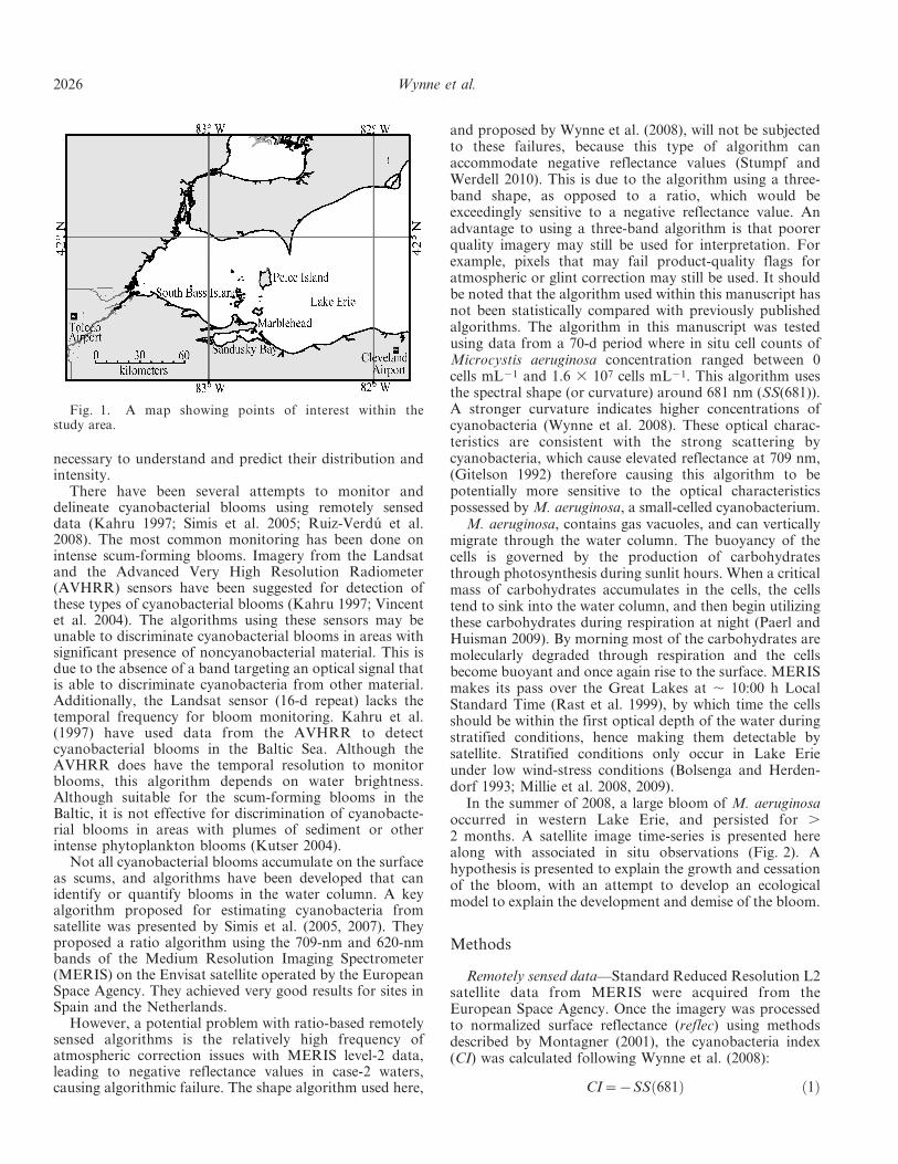
The most common phytoplankton groups found inwestern Lake Erie are chlorophytes, bacillariophytes, andcyanobacteria, together often comprising up to 90% of thetotal chlorophyll a (Chl a; Millie et al. 2009). Chlorophytescan make up to 50% of the phytoplankton Chl a, diatomsas high as 40%, and cyanobacteria between 10% and 30%.The dominant cyanobacterium is generally Microcystisaeruginosa in western Lake Erie, contributing 1–4% of therelative cyanobacterial biomass at the onset of a bloom, butincreasing up to 99% at the height of a bloom (Millie et al.2009; Rinta-Kanto et al. 2009). The exception is inSandusky Bay, where up to 90% of the cyanobacterialbiomass can be comprised of Planktothrix agardii (Fig. 1).These 2 cyanobacterial genera tend to dominate thephytoplankton community during the late summer.

Cyanobacterial blooms develop in warm, stratified watercolumns, with low winds and high light availability (Sellner1997; Carmichael 2008; Paerl and Huisman 2008). They arerelatively slow growing, with doubling periods on the orderof 7 d (Fahnensteil et al. 2008). Intense surface concentra-tion of cyanobacterial blooms may occur because of theirpositive buoyancy (Paerl 1988; Sellner 1997). Watertemperatures above 15uC have been suggested as acontributing factor to the growth and senescence ofcyanobacterial blooms. McQueen and Lean (1987) statedthat cyanobacterial dominance generally occurs whenwater temperatures exceed 20uC. Robarts and Zohary(1987) show that M. aeruginosa populations expand inwater temperatures between 15uC and 25uC. Wind speed,with a threshold of 4 m s21, has been suggested as apossible influence on the intensity of the bloom bychanging its vertical distribution (Hunter et al. 2008).Strong winds mix the cells through the water column.During periods of weak winds, cyanobacteria may float tothe surface, sometimes accumulating in high enoughconcentrations to form scums. Further examination ofcyanobacterial blooms’ response to these factors is* Corresponding author: Timothy.Wynne@noaa.gov

Limnol. Oceanogr., 55(5), 2010, 2025–2036

E 2010, by the American Society of Limnology and Oceanography, Inc.doi:10.4319/lo.2010.55.5.2025

2025

necessary to understand and predict their distribution andintensity.

There have been several attempts to monitor anddelineate cyanobacterial blooms using remotely senseddata (Kahru 1997; Simis et al. 2005; Ruiz-Verdu et al.2008). The most common monitoring has been done onintense scum-forming blooms. Imagery from the Landsatand the Advanced Very High Resolution Radiometer(AVHRR) sensors have been suggested for detection ofthese types of cyanobacterial blooms (Kahru 1997; Vincentet al. 2004). The algorithms using these sensors may beunable to discriminate cyanobacterial blooms in areas withsignificant presence of noncyanobacterial material. This isdue to the absence of a band targeting an optical signal thatis able to discriminate cyanobacteria from other material.Additionally, the Landsat sensor (16-d repeat) lacks thetemporal frequency for bloom monitoring. Kahru et al.(1997) have used data from the AVHRR to detectcyanobacterial blooms in the Baltic Sea. Although theAVHRR does have the temporal resolution to monitorblooms, this algorithm depends on water brightness.Although suitable for the scum-forming blooms in theBaltic, it is not effective for discrimination of cyanobacte-rial blooms in areas with plumes of sediment or otherintense phytoplankton blooms (Kutser 2004).

Not all cyanobacterial blooms accumulate on the surfaceas scums, and algorithms have been developed that canidentify or quantify blooms in the water column. A keyalgorithm proposed for estimating cyanobacteria fromsatellite was presented by Simis et al. (2005, 2007). Theyproposed a ratio algorithm using the 709-nm and 620-nmbands of the Medium Resolution Imaging Spectrometer(MERIS) on the Envisat satellite operated by the EuropeanSpace Agency. They achieved very good results for sites inSpain and the Netherlands.

However, a potential problem with ratio-based remotelysensed algorithms is the relatively high frequency ofatmospheric correction issues with MERIS level-2 data,leading to negative reflectance values in case-2 waters,causing algorithmic failure. The shape algorithm used here,

and proposed by Wynne et al. (2008), will not be subjectedto these failures, because this type of algorithm canaccommodate negative reflectance values (Stumpf andWerdell 2010). This is due to the algorithm using a three-band shape, as opposed to a ratio, which would beexceedingly sensitive to a negative reflectance value. Anadvantage to using a three-band algorithm is that poorerquality imagery may still be used for interpretation. Forexample, pixels that may fail product-quality flags foratmospheric or glint correction may still be used. It shouldbe noted that the algorithm used within this manuscript hasnot been statistically compared with previously publishedalgorithms. The algorithm in this manuscript was testedusing data from a 70-d period where in situ cell counts ofMicrocystis aeruginosa concentration ranged between 0cells mL21 and 1.6 3 107 cells mL21. This algorithm usesthe spectral shape (or curvature) around 681 nm (SS(681)).A stronger curvature indicates higher concentrations ofcyanobacteria (Wynne et al. 2008). These optical charac-teristics are consistent with the strong scattering bycyanobacteria, which cause elevated reflectance at 709 nm,(Gitelson 1992) therefore causing this algorithm to bepotentially more sensitive to the optical characteristicspossessed by M. aeruginosa, a small-celled cyanobacterium.

M. aeruginosa, contains gas vacuoles, and can verticallymigrate through the water column. The buoyancy of thecells is governed by the production of carbohydratesthrough photosynthesis during sunlit hours. When a criticalmass of carbohydrates accumulates in the cells, the cellstend to sink into the water column, and then begin utilizingthese carbohydrates during respiration at night (Paerl andHuisman 2009). By morning most of the carbohydrates aremolecularly degraded through respiration and the cellsbecome buoyant and once again rise to the surface. MERISmakes its pass over the Great Lakes at , 10:00 h LocalStandard Time (Rast et al. 1999), by which time the cellsshould be within the first optical depth of the water duringstratified conditions, hence making them detectable bysatellite. Stratified conditions only occur in Lake Erieunder low wind-stress conditions (Bolsenga and Herden-dorf 1993; Millie et al. 2008, 2009).

In the summer of 2008, a large bloom of M. aeruginosaoccurred in western Lake Erie, and persisted for .2 months. A satellite image time-series is presented herealong with associated in situ observations (Fig. 2). Ahypothesis is presented to explain the growth and cessationof the bloom, with an attempt to develop an ecologicalmodel to explain the development and demise of the bloom.

Methods

Remotely sensed data—Standard Reduced Resolution L2satellite data from MERIS were acquired from theEuropean Space Agency. Once the imagery was processedto normalized surface reflectance (reflec) using methodsdescribed by Montagner (2001), the cyanobacteria index(CI) was calculated following Wynne et al. (2008):

CI~{SS 681ð Þ ð1Þ

Fig. 1. A map showing points of interest within thestudy area.

2026 Wynne et al.

Where the spectral shape (or curvature) is determined as

SS(l)~reflec(l){reflec(l{){freflec(lz){reflec(l{)g

|(l{l{)

(lz{l{)ð2Þ

And l 5 681 nm (MERIS band 8), l+ 5 709 nm (band 9),and l2 5 665 nm (band 7).

This algorithm is an example of a shape algorithmdescribed by Gower et al. (2005). A shape algorithm, suchas that expressed in Eq. 2, reduces to the numerical secondderivative when the bands are evenly spaced, such that(l+ 2 l) 5 (l 2 l2; Schowengerdt 1997; Wynne et al. 2008;Stumpf and Werdell 2010).

The Wynne et al. (2008) method uses a spectral shape,which (unlike ratio algorithms) is insensitive to the presenceof negative radiances. Poor or incomplete atmosphericcorrection also does not influence the results, particularlyas the bands are closely spaced. Gower et al. (2005)developed a similar spectral shape product called theMaximum Chlorophyll Index, using the top-of-atmosphereradiances from MERIS. The algorithm presented by Simiset al. (2005, 2007) is a semianalytic solution, which(although targeted toward phycocyanin) is subject to

failure when used with poor-quality input water reflectance(e.g., negative). Negative reflectance on MERIS may resultfrom inadequacies in either the atmospheric or glintcorrections and their solution is beyond the scope of thisstudy. As a result of the combination of conditions, theWynne et al. (2008) method was applied to all datapresented here. The time series shown in Fig. 2 had avarying amount of negative reflectance pixels recorded,ranging from 2% to 35% of the pixels that the Wynne et al.(2008) method derived as having an elevated Cyanobac-terial Index, with the time-series average of 12.75%.Although it is true that various confidence flags may havebeen turned on in the L2 imagery used, the resultant imagesshown in Fig. 2 show no anomalous features, indicatingthat the algorithm used here may work just as effectivelywith lower quality imagery as it would with higher qualitydata.

A positive CI is indicative of elevated densities ofcyanobacteria. The characteristics of the CI suggest thatit will vary with concentration where a high CI is associatedwith higher density of cyanobacteria (Wynne et al. 2008). Itshould be noted that the algorithm employed here is notable to differentiate between different species of cyanobac-teria. The algorithm may be sensitive to large blooms of

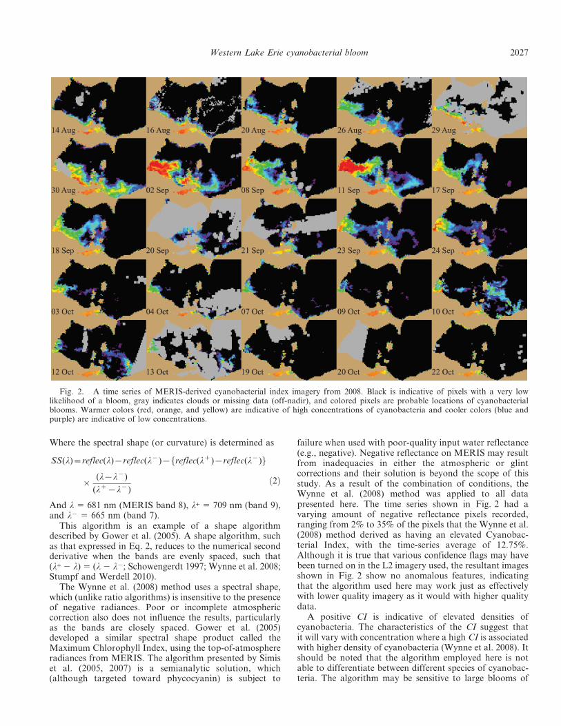
Fig. 2. A time series of MERIS-derived cyanobacterial index imagery from 2008. Black is indicative of pixels with a very lowlikelihood of a bloom, gray indicates clouds or missing data (off-nadir), and colored pixels are probable locations of cyanobacterialblooms. Warmer colors (red, orange, and yellow) are indicative of high concentrations of cyanobacteria and cooler colors (blue andpurple) are indicative of low concentrations.

Western Lake Erie cyanobacterial bloom 2027

other types of phytoplankton, which have the ability toeffectively scatter light.

The SS(681) algorithm uses three bands in the red tonear-infrared portion of the electromagnetic spectrum. Thealgorithm gives an estimate of cyanobacterial biomass inapproximately one optical depth (Gordon and McCluney1975). Gons et al. (2005) suggested that the optical depth ofmost inland waters that have problematic cyanobacterialblooms would be , 0.5 m. The mean specific absorptionfor phytoplankton in Lake Erie is 0.04 m2 mg21 chloro-phyll (Binding et al. 2008). At 10 mg L21 chlorophyll, anoptical depth would be , 1 m at the 660–700-nmwavelengths, whereas pure water has an optical depth of, 2 m in these wavelengths (Pope and Fry 1997).

To quantify the concentration of cyanobacterial cells,the CI was summed for all available pixels in each image.This number was then normalized by the number ofavailable bloom pixels (n 5 4288) for analysis, where abloom pixel is defined as a pixel that had a CI . 0 at somepoint during the 70-d time series presented within thismanuscript (ignoring Sandusky Bay, which was flagged forcyanobacterial blooms throughout the time series). Thisnormalized CI provides an estimate that can be used toderive the intensity of a cyanobacterial bloom for eachimage in the time series. In addition to the density, thenormalized spatial extent (area) of the bloom was found bydetermining the area in each image that had a CI . 0. Thisnumber was then once again normalized by the number ofbloom pixels available (n 5 4288), where a bloom pixel wasdefined as a pixel that had a CI . 0 at some point duringthe 70-d time series shown in Fig. 2 (Fig. 3A).

Cell counts—Surface water samples were collected bygrab sample from 10 to 12 stations throughout westernLake Erie on three separate dates corresponding to clearsatellite imagery: 11 September, 24 September, and 07October 2008. Samples for Microcystis spp. cell countswere preserved with 1% Lugols solution. Once in thelaboratory, 10 mL of sample was gently filtered through a1.2-mm Millipore filter, cleared by adding 50% gluteralde-hyde, heated using a hot plate set to 60uC, dried overnight,and then mounted to a slide using Permount, according toDozier and Richerson (1975). Microcystis colonies withcells of 3–5 mm in diameter (Komarek and Anagnostidis1999) were counted. Measurements were made of the areaof the colony, minus peripheral mucilage and emptyinterior spaces. From these values, biovolume and thenequivalent spherical diameter (ESD) were calculatedaccording to the methods of Hillebrand et al. (1999). Fromthe colony ESD, cell number was calculated based on anempirical relationship derived from sonicating individualMicrocystis colonies from western Lake Erie and enumer-ating cell numbers in those colonies (Dyble et al. 2008). Cellnumber was calculated as

log Y~2:83 log10Xð Þ{2:50 ð3Þ

where Y is the cell number in cells mL21 (Y), and X is thecolony ESD. This method of cell counting has an error of20% associated with it (Reynolds and Jaworski 1978).

Wind data—Hourly meteorological observations weredownloaded from the National Oceanic and AtmosphericAdministration (NOAA) National Data Buoy Center(NDBC) Sta. SBI01, located on South Bass Island, Ohio,U.S.A. (41.628 N 82.842 W; Fig. 1). Wind stress (t) wascalculated using

t~r|CD|w2 ð4Þ

where r is the density of air, estimated to be 1.25 kg m23,and CD is the drag coefficient determined by (Hsu 1973):

CD~0:001|(0:69z0:081|w), ð5Þ

and w is the mean hourly wind speed.An average wind stress was calculated by using the wind

speeds from the 24 h preceding the time of a satellite image(Fig. 3B). Wind stress was used as it is expressed as a force,and a force is needed to drive the advective mixing neededto de-stratify the water column.

Water temperature—Water temperatures were obtainedfrom the NOAA Center for Operational Products andServices (CO-OPS) Sta. 9063079, located at Marblehead,Ohio (41.545 N, 82.732 W). The 24-h mean watertemperature was calculated from hourly observational datain the same fashion as for the winds (Fig. 3C).

Light availability (sun index)—To estimate light avail-ability, the average sky cover between sunrise and sunset,reported in tenths of sky covered by clouds, was obtainedfrom the National Weather Service for the Toledo ExpressAirport and Cleveland Hopkins International Airport(http://www.weather.gov/climate/index.php?wfo5cle). TheNational Weather Service reports 100% cloud-cover as 10and clear conditions as 0. The inverse of this index was usedfor this study, because the desired value was the percentageof sun present and not the amount of clouds. The resultantindex will be referred to as the ‘sun index,’ with a value of10 indicating clear skies with 0% cloud cover, and a valueof 0 indicating 100% cloud cover. The Toledo airport is tothe west of the bloom area, and the Cleveland airport is tothe southeast of the bloom area (Fig. 1). A mean wascalculated using the two stations in an effort to try andestimate the sun conditions in the area around the bloom(Fig. 3D). It should be noted that the Toledo airportgenerally experienced clearer skies throughout the timeseries relative to the Cleveland airport.

Results

Field validation—Cell counts from 3 d (11 Sep, 24 Sep,and 03 Oct 08) were compared with the satellite derived CI.These cell counts were from same-day match-ups. Cyano-bacterial blooms are extremely patchy at subpixel scales(Kutser et al. 2008). In the data collected for this study, twopoints were collected from one station (latitude 41.7919,longitude 283.3925) on 28 August (data not shown becauseno image was available for this date). The cell counts fromthese two samples varied in concentration by an order ofmagnitude (3.6 3 105–3.7 3 106 cells mL21), illustrating the

2028 Wynne et al.

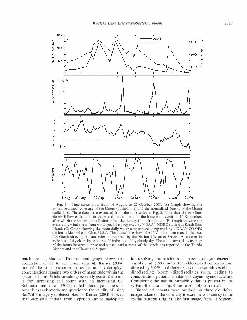
patchiness of blooms. The resultant graph shows thecorrelation of CI to cell count (Fig. 4). Kutser (2004)noticed the same phenomenon, as he found chlorophyllconcentrations ranging two orders of magnitude within thespace of 1 km2. While variability certainly exists, the trendis for increasing cell count with an increasing CI.Subramanium et al. (2002) noted bloom patchiness inoceanic cyanobacteria and questioned the validity of usingSeaWiFS imagery to detect blooms. Kutser (2004) showedthat 30-m satellite data (from Hyperion) can be inadequate

for resolving the patchiness in blooms of cyanobacteria.Yacobi et al. (1995) noted that chlorophyll concentrationsdiffered by 300% on different sides of a research vessel in adinoflagellate bloom (dinoflagellates swim, leading toconcentration patterns similar to buoyant cyanobacteria).Considering the natural variability that is present in thesystem, the data in Fig. 4 are reasonably correlated.

Binned cell counts were overlaid on three cloud-freeimages taken on the same day to examine consistency in thespatial patterns (Fig. 5). The first image, from 11 Septem-

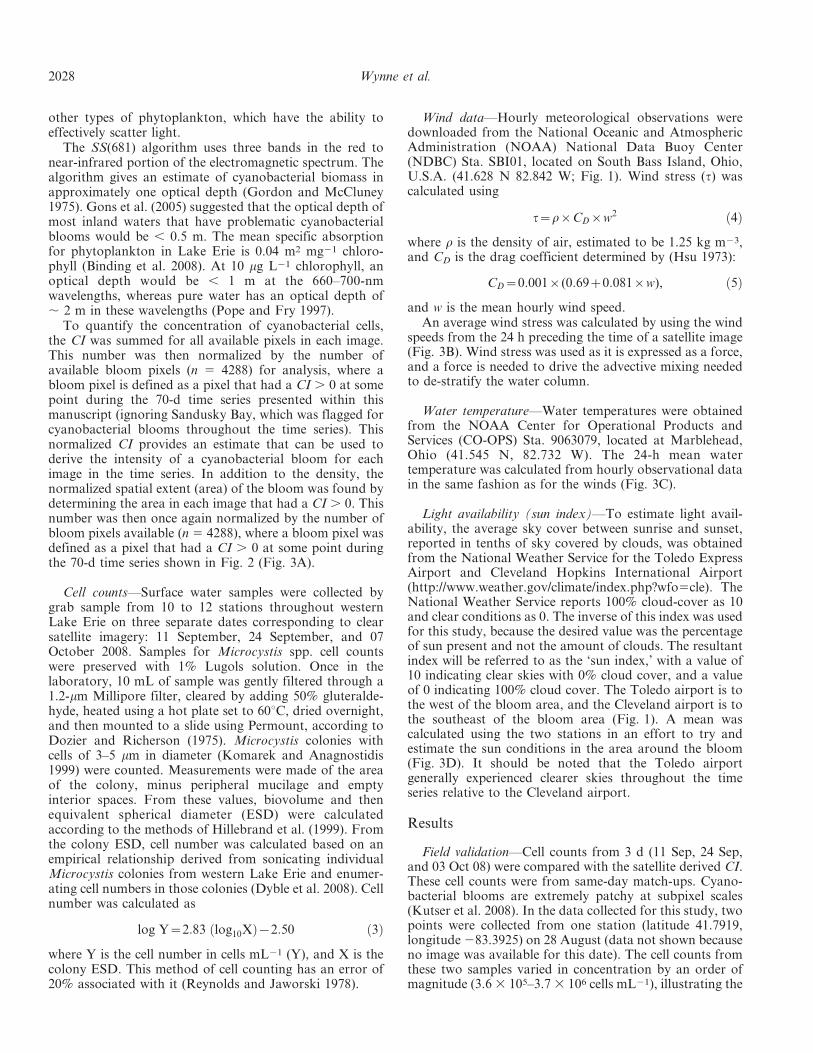
Fig. 3. Time series plots from 14 August to 22 October 2008. (A) Graph showing thenormalized areal coverage of the bloom (dashed line) and the normalized density of the bloom(solid line). These data were extracted from the time series in Fig. 2. Note that the two linesclosely follow each other in shape and magnitude until the large wind event on 15 September,after which the shapes are still similar but the density is much reduced. (B) Graph showing themean daily wind stress from wind-speed data reported by NOAA’s NDBC station at South BassIsland. (C) Graph showing the mean daily water temperature as reported by NOAA’s CO-OPSstation at Marblehead, Ohio, U.S.A. The dashed line shows the 15uC point mentioned in the text.(D) Graph showing the sun index, as reported by the National Weather Service. A score of 10indicates a fully clear sky. A score of 0 indicates a fully cloudy sky. These data are a daily averageof the hours between sunrise and sunset, and a mean of the conditions reported at the ToledoAirport and the Cleveland Airport.

Western Lake Erie cyanobacterial bloom 2029

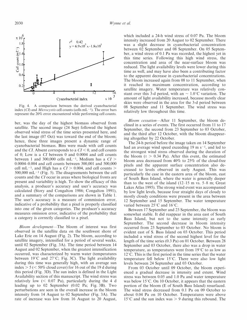
ber, was the day of the highest biomass observed fromsatellite. The second image (24 Sep) followed the highestobserved wind stress of the time series presented here, andthe last image (07 Oct) was toward the end of the bloom;hence, these three images present a dynamic range ofcyanobacterial biomass. Bins were made with cell countsand the CI. Absent corresponds to a CI , 0, and cell countsof 0; Low is a CI between 0 and 0.0004 and cell countsbetween 1 and 300,000 cells mL21, Medium has a CI .0.0004–0.004 and cell counts between 300,001 and 500,000cell mL21, and High has a CI . 0.004, and cell counts .500,000 mL21 (Fig. 5). The disagreements between the cellcounts and the CI occur in areas where biological fronts arepresent and variability is high. To show the efficacy of thisanalysis, a producer’s accuracy and user’s accuracy wascalculated (Story and Congalton 1986; Congalton 1991),and a summary of the comparisons are shown in Table 1.The user’s accuracy is a measure of commission error,indicative of a probability that a pixel is properly classifiedinto one of the given categories. The producer’s accuracymeasures omission error, indicative of the probability thata category is correctly classified to a pixel.

Bloom development—The bloom of interest was firstobserved in the satellite data on the southwest shore ofLake Erie on 14 August (Fig. 2). The bloom, according tosatellite imagery, intensified for a period of several weeks,until 02 September (Fig. 3A). The time period between 14August and 02 September, when the greatest intensificationoccurred, was characterized by warm water (temperaturesbetween 19uC and 27uC; Fig. 3C). The light availabilityduring this time was generally high, with an average sunindex . 5 (, 50% cloud cover) for 16 out of the 19 d duringthis period (Fig. 3D). The sun index is defined in the LightAvailability section of this manuscript. The wind stress wasrelatively low (, 0.07 Pa), particularly during the 4 dleading up to 02 September (0.02 Pa; Fig. 3B). Twoperturbations are seen in the overall increase in the bloomintensity from 14 August to 02 September (Fig. 3A). Therate of increase was low from 16 August to 20 August,

which included a 24-h wind stress of 0.07 Pa. The bloomintensity increased from 20 August to 02 September. Therewas a slight decrease in cyanobacterial concentrationbetween 02 September and 08 September. On 05 Septem-ber, a wind stress of 0.1 Pa was recorded, the highest yet inthis time series. Following this high wind stress, theconcentration and area of the near-surface bloom wasreduced. The light availability levels were lower during thistime as well, and may have also been a contributing factorto the apparent decrease in cyanobacterial concentrations.The bloom increased again from 08 to 11 September, whenit reached its maximum concentration, according tosatellite imagery. Water temperature was relatively con-stant over this 3-d period, with an , 1.0uC variation. Theamount of light availability increased, because mostly clearskies were observed in the area for the 3-d period between08 September and 11 September. The wind stress wasrelatively low throughout this time.

Bloom cessation—After 11 September, the bloom de-clined in a series of events. The first occurred from 11 to 17September, the second from 23 September to 03 October,and the third after 12 October, with the bloom disappear-ing altogether by 22 October.

The 24-h period before the image taken on 14 Septemberhad an average wind speed exceeding 19 m s21, and led tothe strongest wind stress observed during the duration ofthe bloom (t . 0.34 Pa). After this event, the estimatedbloom area decreased from 40% to 25% of the cloud-freepixels and the apparent surface concentration also de-creased to levels observed in early August. This wasparticularly the case in the eastern area of the bloom, eastof South Bass Island, where the water is generally deeperthan to the west of the island (12–15 m vs. 5–8 m; GreatLakes Atlas 1995). The strong wind event was accompaniedby low light levels, because four straight days of cloudy tomostly cloudy conditions were present in the area between12 September and 15 September. The water temperaturevaried between 25uC and 16uC.

Between 17 September and 23 September, the bloom wassomewhat stable. It did reappear in the area east of SouthBass Island, but not to the same intensity as earlySeptember. The second decrease in bloom intensityoccurred from 23 September to 03 October. No bloom isevident east of S. Bass Island on 03 October. This periodincluded a wind stress of the second highest level for thelength of the time series (0.3 Pa) on 01 October. Between 28September and 03 October, there also was a drop in watertemperature, as temperatures went from 19uC to as low as12uC. This is the first period in the time series that the watertemperature fell below 15uC. There were also low lightlevels between 24 September and 03 October.

From 03 October until 09 October, the bloom experi-enced a gradual decrease in intensity and extent. Windstress was between 0.05 and 1.0 Pa and water temperaturewas below 15uC. On 10 October, it appears that the easternportion of the bloom (E of South Bass Island) resurfaced.The wind stress decreased from 0.1 Pa on 09 October toabout 0.04 Pa on 10 October. Temperatures were above15uC and the sun index was . 9 during this rebound. The

Fig. 4. A comparison between the derived cyanobacterialindex (CI) and Microcystis cell counts (cells mL21). The error barsrepresent the 20% error encountered while performing cell counts.

2030 Wynne et al.

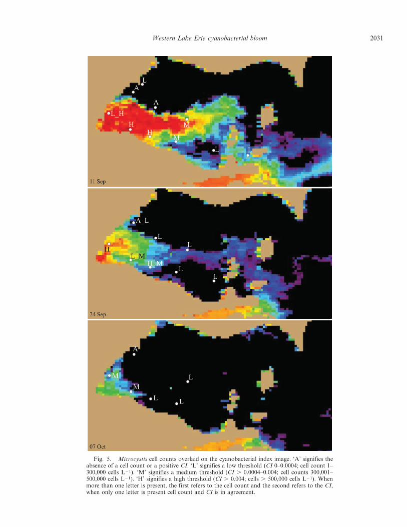
Fig. 5. Microcystis cell counts overlaid on the cyanobacterial index image. ‘A’ signifies theabsence of a cell count or a positive CI. ‘L’ signifies a low threshold (CI 0–0.0004; cell count 1–300,000 cells L21). ‘M’ signifies a medium threshold (CI . 0.0004–0.004; cell counts 300,001–500,000 cells L21). ‘H’ signifies a high threshold (CI . 0.004; cells . 500,000 cells L21). Whenmore than one letter is present, the first refers to the cell count and the second refers to the CI,when only one letter is present cell count and CI is in agreement.

Western Lake Erie cyanobacterial bloom 2031

eastern bloom was visible from 10 to 13 October. Thiscorresponds to a time when the wind stress was low and thetemperature remained above 15uC.

The last event after 12 October resulted in thedisappearance of the bloom by 22 October. The interveningtime had a wind event of 0.1 Pa, with water temperaturesbelow 11uC and low sun index. The western portion of thebloom, near the mouth of the Maumee River, decreasedfrom 10 to 19 October and was no longer visible on or after22 October.

Discussion

The MERIS satellite imagery, in combination with thephysical data presented here of wind stress, watertemperature, and light availability, was effective incharacterizing the Microcystis bloom in western Lake Erieduring the summer and autumn of 2008.

Wind—The decreases in bloom area and intensityoccurred after daily wind stresses exceeded 0.1 Pa (equatingto a wind speed of , 7.7 m s21). This is generally higherthen observations made by George and Edwards (1976),who noted that wind speeds in excess of 4 m s21 (0.02 Pa)were sufficient to cause buoyant cyanobacteria to be sub-merged below the surface. Hunter et al. (2008) noted thatthe blooms of M. aeruginosa were driven to depth by windspeeds of 6 m s21 (0.053 Pa). It should be noted that in bothof these examples the water bodies under considerationwere small and shallow relative to the western basin ofLake Erie. The lake that Hunter et al. (2008) examined(Barton Broad, U.K.) had an average depth of 1.2 m.Because western Lake Erie is much deeper (, 5–15 m), itwould be expected that a stronger wind stress would berequired to mix the bloom through the water column,because generally deeper water will be more stratified andrequire a greater stress for mixing. Western Lake Erie mayhave a modest thermocline, which must be overcome forcells to be mixed throughout the water column.

A wind event of 0.1 Pa appears consistent with a mixingevent that is strong enough to submerge the cells to reducedor even undetectable levels (from satellite) in Lake Erie.The trend can be seen throughout the time series where thewind stress exceeded 0.1 Pa. For example, a decrease inbloom area and concentration occurred after the strongestwind event of the observed period (0.34 Pa on 15 Sep). Thebloom never fully recovered after this point, which mayhave partially been due to reduced light availability atdepth and decreasing temperature, as described below. The

water may have not fully restratified after this event,thereby allowing smaller wind stresses the ability to mix thecells homogeneously through the water and not allowingremote detection.

Conversely, in late August, the normalized area anddensity tended to increase during periods of low wind stress(, 0.05 Pa). Wind stress between 0.05 and 0.1 Pa appearedto slow this intensification. This probably results frompartial mixing of the bloom into the water column resultingin a real decrease in surface concentration, and an apparentdecrease in bloom area.

Gons et al. (2005) made note that the near-surfaceconcentration of Microcystis will be higher during periodsof low wind stress, and that during periods of high windstress, the cells will be homogeneously mixed throughoutthe water column. It appears that the same factors areapplied to the case of this bloom. The satellite may give anaccurate representation of the biomass during mixedconditions provided that the bathymetry is accounted for(Wynne et al. 2006). However, without knowledge of thevertical distribution of the cells it will be impossible todetermine this.

Temperature—Water temperature has been hypothesizedas a key factor in the growth and cessation of cyanobacte-rial blooms (Paerl 1988; Sellner 1997; Paerl and Huisman2008). In this study, rapid expansion and intensification ofthe bloom occurred during a period with water temperature. 19uC. On 01 October, the temperature fell below thethreshold for algal bloom development of 15uC proposedby Robarts and Zohary (1987) for the first time in theconsidered time series. The combination of temperatureand wind appeared to weaken the bloom. There wasrecovery of the areal coverage of the bloom, but not ofbloom intensity (Fig. 3A). After 13 October, the bloom didnot recover despite low wind stress. A series of high wind-stress events (09, 16, and 21 Oct) and temperatures below15uC may have prevented the recovery of the bloom, evenduring periods of low wind stress, eventually leading tobloom cessation.

Light—Light availability may play a slight role in theformation and cessation of blooms; however, any influenceis obscured by the association of bloom density with windstress and water temperature during the study perioddiscussed here. This may change as a function of season.Generally, the bloom described in this manuscript grewwith clearer skies and subsided with cloudier skies. Thismay be due to confounding factors. Clear sunny skies were

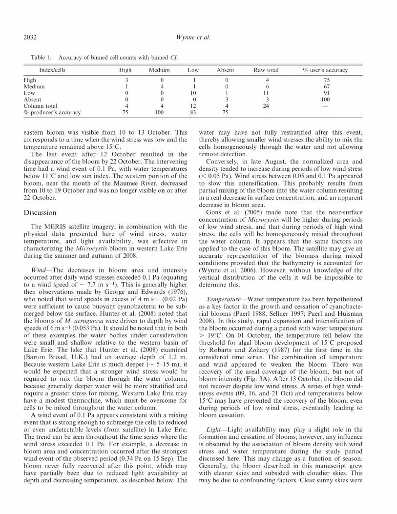
Table 1. Accuracy of binned cell counts with binned CI.

Index/cells High Medium Low Absent Raw total % user’s accuracy

High 3 0 1 0 4 75Medium 1 4 1 0 6 67Low 0 0 10 1 11 91Absent 0 0 0 3 3 100Column total 4 4 12 4 24 —% producer’s accuracy 75 100 83 75 — —

2032 Wynne et al.

accompanied by periods of low wind stress and warm watertemperatures, and periods of cloudy skies were accompa-nied by periods of high wind stress. It is possible that thelight is the driving factor to the reduction in cyanobacterialbloom intensity. However, the hypothesis presented hereindicates that the wind stress is the driving factor andreduction in bloom intensity on satellite imagery is due tothe bloom being mixed through the water column, therebyreducing the concentration in the first optical depth (upper1 m). The data presented in the time series in Fig. 3 supportthis hypothesis. Comparing the Sun Index with bloom areaand extent (Fig. 3A) shows some mismatches. On 28August the sun index is reported as 1, (90% clouds), whichhad no apparent adverse effect on the concentration ofbloom-forming cells or area. The same trend is seen at theend of the time series, when 19 October, a clear day withlittle wind, had no positive effect on the concentration orextent of the bloom.

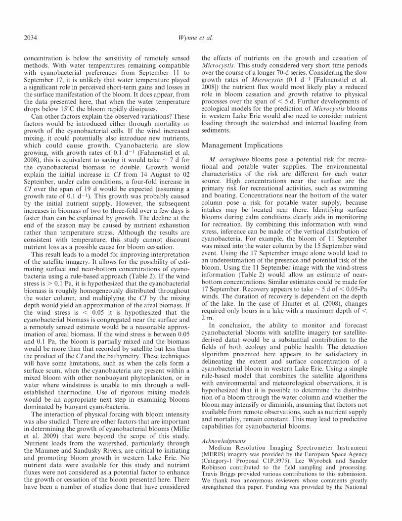
Interpretations of observations—The use of satelliteimagery to observe cyanobacterial blooms is hypothesizedto be modulated by wind and temperature conditions(Table 2). In using satellite imagery to characterizecyanobacterial bloom intensity, wind stress is hypothesizedas the dominant factor, but is modulated by the watertemperature. Wind stress may provide a potential indicatorto describe how the bloom is distributed through the watercolumn. Under weak wind there will not be the neededturbulence to mix the cells, thereby allowing them tocongregate at the surface. Thus, the satellite should be ableto deliver a more accurate representation of the arealbiomass (Gons et al. 2005; Hunter et al. 2008). During highwind-stress conditions, satellite imagery will provide near-surface (, 1 m) concentrations. However, the total arealbiomass of the bloom will be underestimated because thecells will be mixed throughout the water column.

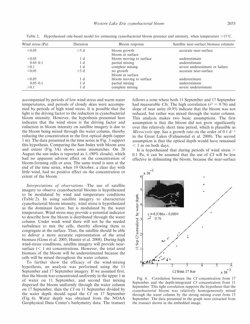
To further show the efficacy of the wind-mixinghypothesis, an analysis was performed using the 11September and 17 September imagery. If we assumed first,that the bloom was concentrated uniformly in the upper 1 mof water on 11 September, and second that mixingdispersed the bloom uniformly through the water columnon 17 September, then the CI on 11 September divided bythe water depth should equal the CI on 17 September(Fig. 6). Water depth was obtained from the NOAAGeophysical Data Center’s bathymetry data. The transect

follows a zone where both 11 September and 17 Septemberhad measurable CIs. The high correlation (r2 5 0.76) andslope of near unity (0.95) indicate that the bloom was notreduced, but rather was mixed through the water column.This analysis makes two basic assumptions. The firstassumption is that the bloom did not grow significantlyover this relatively short time period, which is plausible asMicrocystis spp. has a growth rate on the order of 0.1 d21

in the Great Lakes (Fahnenstiel et al. 2008). The secondassumption is that the optical depth would have remained, 1 m on both days.

It is hypothesized that during periods of wind stress .0.1 Pa, it can be assumed that the use of CI will be lesseffective in delineating the bloom, because the near-surface

Table 2. Hypothesized rule-based model for estimating cyanobacterial bloom presence and intensity, when temperature .15uC.

Wind stress (Pa) Duration Bloom response Satellite near-surface biomass estimate

,0.05 .5 d bloom growth accurate near-surfacebloom at surface

,0.05 1 d bloom moving to surface underestimate0.05–0.1 1 d partial mixing underestimate

.0.1 1 d complete mixing severe underestimate or failure,0.05 .5 d no growth accurate near-surface

bloom at surface,0.05 1 d bloom moving to surface underestimate

0.05–0.1 1 d partial mixing underestimate.0.1 1 d complete mixing severe underestimate

Fig. 6. Correlation between the CI concentration from 17September and the depth-integrated CI concentration from 11September. This tight correlation supports the hypothesis that thecyanobacterial bloom was relatively homogeneously mixedthrough the water column by the strong mixing event from 15September. The data presented in the graph were extracted fromthe transect shown in the embedded image.

Western Lake Erie cyanobacterial bloom 2033

concentration is below the sensitivity of remotely sensedmethods. With water temperatures remaining compatiblewith cyanobacterial preferences from September 11 toSeptember 17, it is unlikely that water temperature playeda significant role in perceived short-term gains and losses inthe surface manifestation of the bloom. It does appear, fromthe data presented here, that when the water temperaturedrops below 15uC the bloom rapidly dissipates.

Can other factors explain the observed variations? Thesefactors would be introduced either through mortality orgrowth of the cyanobacterial cells. If the wind increasedmixing, it could potentially also introduce new nutrients,which could cause growth. Cyanobacteria are slowgrowing, with growth rates of 0.1 d21 (Fahnenstiel et al.2008), this is equivalent to saying it would take , 7 d forthe cyanobacterial biomass to double. Growth wouldexplain the initial increase in CI from 14 August to 02September, under calm conditions, a four-fold increase inCI over the span of 19 d would be expected (assuming agrowth rate of 0.1 d21). This growth was probably causedby the initial nutrient supply. However, the subsequentincreases in biomass of two to three-fold over a few days isfaster than can be explained by growth. The decline at theend of the season may be caused by nutrient exhaustionrather than temperature stress. Although the results areconsistent with temperature, this study cannot discountnutrient loss as a possible cause for bloom cessation.

This result leads to a model for improving interpretationof the satellite imagery. It allows for the possibility of esti-mating surface and near-bottom concentrations of cyano-bacteria using a rule-based approach (Table 2). If the windstress is . 0.1 Pa, it is hypothesized that the cyanobacterialbiomass is roughly homogeneously distributed throughoutthe water column, and multiplying the CI by the mixingdepth would yield an approximation of the areal biomass. Ifthe wind stress is , 0.05 it is hypothesized that thecyanobacterial biomass is congregated near the surface anda remotely sensed estimate would be a reasonable approx-imation of areal biomass. If the wind stress is between 0.05and 0.1 Pa, the bloom is partially mixed and the biomasswould be more than that recorded by satellite but less thanthe product of the CI and the bathymetry. These techniqueswill have some limitations, such as when the cells form asurface scum, when the cyanobacteria are present within amixed bloom with other nonbuoyant phytoplankton, or inwater where windstress is unable to mix through a well-established thermocline. Use of rigorous mixing modelswould be an appropriate next step in examining bloomsdominated by buoyant cyanobacteria.

The interaction of physical forcing with bloom intensitywas also studied. There are other factors that are importantin determining the growth of cyanobacterial blooms (Millieet al. 2009) that were beyond the scope of this study.Nutrient loads from the watershed, particularly throughthe Maumee and Sandusky Rivers, are critical to initiatingand promoting bloom growth in western Lake Erie. Nonutrient data were available for this study and nutrientfluxes were not considered as a potential factor to enhancethe growth or cessation of the bloom presented here. Therehave been a number of studies done that have considered

the effects of nutrients on the growth and cessation ofMicrocystis. This study considered very short time periodsover the course of a longer 70-d series. Considering the slowgrowth rates of Microcystis (0.1 d21 [Fahnenstiel et al.2008]) the nutrient flux would most likely play a reducedrole in bloom cessation and growth relative to physicalprocesses over the span of , 5 d. Further developments ofecological models for the prediction of Microcystis bloomsin western Lake Erie would also need to consider nutrientloading through the watershed and internal loading fromsediments.

Management Implications

M. aeruginosa blooms pose a potential risk for recrea-tional and potable water supplies. The environmentalcharacteristics of the risk are different for each watersource. High concentrations near the surface are theprimary risk for recreational activities, such as swimmingand boating. Concentrations near the bottom of the watercolumn pose a risk for potable water supply, becauseintakes may be located near there. Identifying surfaceblooms during calm conditions clearly aids in monitoringfor recreation. By combining this information with windstress, inference can be made of the vertical distribution ofcyanobacteria. For example, the bloom of 11 Septemberwas mixed into the water column by the 15 September windevent. Using the 17 September image alone would lead toan underestimation of the presence and potential risk of thebloom. Using the 11 September image with the wind-stressinformation (Table 2) would allow an estimate of near-bottom concentrations. Similar estimates could be made for17 September. Recovery appears to take , 5 d of , 0.05-Pawinds. The duration of recovery is dependent on the depthof the lake. In the case of Hunter et al. (2008), changesrequired only hours in a lake with a maximum depth of ,2 m.

In conclusion, the ability to monitor and forecastcyanobacterial blooms with satellite imagery (or satellite-derived data) would be a substantial contribution to thefields of both ecology and public health. The detectionalgorithm presented here appears to be satisfactory indelineating the extent and surface concentration of acyanobacterial bloom in western Lake Erie. Using a simplerule-based model that combines the satellite algorithmswith environmental and meteorological observations, it ishypothesized that it is possible to determine the distribu-tion of a bloom through the water column and whether thebloom may intensify or diminish, assuming that factors notavailable from remote observations, such as nutrient supplyand mortality, remain constant. This may lead to predictivecapabilities for cyanobacterial blooms.

AcknowledgmentsMedium Resolution Imaging Spectrometer Instrument

(MERIS) imagery was provided by the European Space Agency(Category-1 Proposal C1P.3975). Lee Wyrobek and SanderRobinson contributed to the field sampling and processing.Travis Briggs provided various contributions to this submission.We thank two anonymous reviewers whose comments greatlystrengthened this paper. Funding was provided by the National

2034 Wynne et al.

Oceanic and Atmospheric Administration’s (NOAA) Center ofExcellence for Great Lakes and Human Health, and through theNational Center for Environmental Health at the Centers forDisease Control and Prevention and by the NASA AppliedScience Program announcement NNH08ZDA001N under con-tract NNH09AL53I.

References

BINDING, C. E., J. H. JEROME, R. P. BUKATA, AND W. G. BOOTY.2008. Spectral absorption of dissolved and particulate matterin Lake Erie. Remote Sens. Environ. 112: 1702–1711.

BOLSENGA, S. J., AND C. E. HERDENDORF. 1993. Lake Erie andLake St. Claire handbook. Wayne State Univ. Press.

BRITTAIN, S. M., J. WANG, L. BABCOCK-JACKSON, W. W.CARMICHAEL, K. L. RINEHART, AND D. A. CULVER. 2000.Isolation and characterization of microcystins, cyclic hepato-toxins from Lake Erie strains of Microcystis aeruginosa.J. Gt. Lakes Res. 26: 241–249, doi:10.1016/S0380-1330(00)70690-3

BUDD, J. W., T. D. DRUMMER, T. F. NALEPA, AND G. L.FAHNENSTIEL. 2001. Remote sensing of biotic effects: Zebramussels (Dreissena polymorpha) influence on water clarity inSaginaw Bay, Lake Huron. Limnol. Oceanogr. 46: 213–223.

CARMICHAEL, W. W. 1992. A status report on planktoniccyanobacteria (blue green algae) and their toxins. U.S.Environmental Protection Agency, Environmental Monitor-ing Systems Laboratory, Office of Research and Develop-ment.

———. 1998. Algal poisoning, p. 2022–2023. In S. Aiello [ed.],The Merck veterinary manual. Merck.

———. 2008. A world overview one-hundred, twenty-seven yearsof research on toxic cyanobacteria—where do we go fromhere? Adv. Exp. Med. Biol. 619: 105–125, doi:10.1007/978-0-387-75865-7_4

CONGALTON, R. G. 1991. A review of Assessing the accuracy ofclassifications of remotely sensed data. Remote Sens. Envi-ron. 37: 35–46, doi:10.1016/0034-4257(91)90048-B

DOZIER, B. J., AND P. J. RICHERSON. 1975. An improved membranefilter method for the enumeration of phytoplankton. Verh.Int. Ver. Limnol. 19: 1524–1529.

DYBLE, J., G. L. FAHNENSTIEL, R. W. LITAKER, D. F. MILLIE, AND

P. A. TESTER. 2008. Microcystin concentrations and geneticdiversity of Microcystis in the lower Great Lakes. Environ.Toxicol. 23: 507–516, doi:10.1002/tox.20370

FAHNENSTIEL, G. L., AND oTHERS. 2008. Factors affectingmicrocystin concentration and cell quota in Saginaw Bay,Lake Huron. Aquat. Ecosyst. Health Manag. 11: 190–195,doi:10.1080/14634980802092757

GEORGE, D. G., AND R. W. EDWARDS. 1976. The effect of wind onthe distribution of chlorophyll-a and crustacean plankton in ashallow eutrophic reservoir. J. Appl. Ecol. 13: 667–690,doi:10.2307/2402246

GITELSON, A. 1992. The peak near 700 nm on radiance spectra ofalgae and water: Relationships of its magnitude and positionwith chlorophyll concentration. Int. J. Remote Sens. 13:3367–3373, doi:10.1080/01431169208904125

GONS, H. J., H. HAKVOORT, S. W. M. PETERS, AND S. G. H. SIMIS.2005. Optical detection of cyanobacterial blooms, p. 177–199.In J. Huisman, H. C. P. Matthijs and P. M. Visser [eds.],Harmful cyanobacterial. Springer.

GORDON, H. R., AND W. R. MCCLUNEY. 1975. Estimation of thedepth of sunlight penetration in the sea for remote-sensing.Appl. Optics 14: 413–416, doi:10.1364/AO.14.000413

GOWER, J., S. KING, G. BORSTAD, AND L. BROWN. 2005. Detectionof intense plankton blooms using the 709nm band of theMERIS imaging spectrometer. Int. J. Remote Sens. 26:2005–2021, doi:10.1080/01431160500075857

GREAT LAKES ATLAS. 1995. Jointly produced by the Governmentof Canada and U.S. Environmental Protection Agency[accessed 24 July 2008]. Available online at: http://www.epa.gov/glnpo/atlas/index.html.

HAWKINS, P. R., M. T. C. RUNNEGAR, A. R. B. JACKSON, AND I. R.FALCONER. 1985. Severe heptatoxicity caused by the tropicalcyanobacterium (blue-green alga) Cylindrospermopsis raci-borskii (Woloszynska). Seenayya and Subba Raju isolatedfrom a domestic water supply reservoir. Appl. Environ.Microb. 50: 1292–1295.

HILLEBRAND, H., C. D. DURSELEN, D. KIRSCHTEL, U. POLLINGHER,AND T. ZOHARY. 1999. Biovolume calculation for pelagic andbenthic microalgae. J. Phycol. 35: 403–424, doi:10.1046/j.1529-8817.1999.3520403.x

HSU, S. A. 1973. Experimental results of the drag-coefficientestimation for air–coast interfaces. Bound.-Lay. Meteorol. 6:505–507, doi:10.1007/BF02137682

HUNTER, P. D., A. N. TYLER, N. J. WILLBY, AND D. J. GILVEAR.2008. The spatial dynamics of vertical migration by Micro-cystis aeruginosa in a eutrophic shallow lake: A case studyusing high spatial resolution time-series airborne remotesensing. Limnol. Oceanogr. 53: 2391–2406.

IBELINGS, B. W., M. VONK, H. F. J. LOS, D. T. VAN DER MOLEN,AND W. M. MOOIJ. 2003. Fuzzy modeling of cyanobacterialsurface waterblooms: Validation with NOAA-AVHRR satel-lite images. Ecol. Appl. 13: 1456–1472, doi:10.1890/01-5345

JUHEL, G., AND oTHERS. 2006. Pseudodiarrhoea in zebra musselsDreissena polymorpha (Pallas) exposed to microcystins. J.Exp. Biol. 209: 810–816, doi:10.1242/jeb.02081

KAHRU, M. 1997. Using satellites to monitor large-scale environ-mental change in the Baltic Sea, p. 43–61. In M. Kahru and C.W. Brown [eds.], Monitoring algal blooms: New techniquesfor detecting large-scale environmental change. Springer-Verlag.

KOMAREK, J., AND K. ANAGNOSTIDIS. 1999. Cyanoprokaryota: Teilchroococcales, p. 1–548. In A. Pasher, H. Ettl, G. Gartner, H.Heynig and D. Mollenhauer [eds.], Subwasserflora vonMilleleuropa. Gustay Fischer.

KUIPER-GOODMAN, T., I. R. FALCONER, AND J. FITZGERALD. 1999.Human health aspects, p. 113–153. In I. Chorus and J.Bartram [eds.], Toxic cyanobacteria in water. A guide to theirpublic health consequences, monitoring and management.World Health Organization.

KUTSER, T. 2004. Quantitative detection of chlorophyll incyanobacterial blooms by satellite remote sensing. Limnol.Oceanogr. 49: 2179–2189.

———, L. METSAMAA, AND A. G. DEKKER. 2008. Influence of thevertical distribution of cyanobacteria in the water column onthe remote sensing signal. Estuar. Coast. Shelf Sci. 78:649–654, doi:10.1016/j.ecss.2008.02.024

MCQUEEN, D. J., AND D. R. S. LEAN. 1987. Influence of watertemperature and nitrogen to phosphorus ratios on thedominance of blue-green in Lake St. George, Ontario. Can.J. Fish. Aquat. Sci. 44: 598–604, doi:10.1139/f87-073

MILLIE, D. F., AND oTHERS. 2008. Influence of environmentalconditions on late-summer cyanobacterial abundance inSaginaw Bay, Lake Huron. Aquat. Ecosyst. Health Manag.11: 196–205, doi:10.1080/14634980802099604

———, AND OTHERS. 2009. Late-summer phytoplankton inwestern Lake Erie (Laurentian Great Lakes): Bloom distri-butions, toxicity, and environmental influences. Aquat. Ecol.43: 915–934, doi:10.1007/s10452-009-9238-7

Western Lake Erie cyanobacterial bloom 2035

MONTAGNER, F. 2001. Reference model for MERIS level 2processing. European Space Agency, document No. PO-TN-MEL-GS-0026.

PAERL, H. W. 1988. Nuisance phytoplankton blooms in coastal,estuarine, and inland waters. Limnol. Oceanogr. 33: 823–847,doi:10.4319/lo.1988.33.4_part_2.0823

———, AND J. HUISMAN. 2008. Blooms like it hot. Science 320:57–58, doi:10.1126/science.1155398

———, AND ———. 2009. Climate change: A catalyst forglobal expansion of harmful cyanobacterial blooms.Environ. Microbiol. Rep. 1: 27–37, doi:10.1111/j.1758-2229.2008.00004.x

POPE, R. M., AND E. S. FRY. 1997. Absorption spectrum(380–700 nm) of pure water. II. Integrating cavity measure-ments. Appl. Optics 36: 8710–8723, doi:10.1364/AO.36.008710

RAST, M., J. L. BEZY, AND S. BRUZZI. 1999. The ESA mediumresolution imaging spectrometer MERIS: A review of theinstrument and its mission. Int. J. Remote Sens. 20:1681–1702, doi:10.1080/014311699212416

REYNOLDS, C. S., AND G. H. M. JAWORSKI. 1978. Enumeration ofnatural Microcystis populations. Br. Phycol. J. 13: 269–277,doi:10.1080/00071617800650331

RINTA-KANTO, J. M., E. A. KONOPKO, J. M. DEBRUYN, R. A.BOURBONNIERE, G. L. BOYER, AND S. W. WILHELM. 2009. LakeErie Microcystis: Relationship between microcystin produc-tion, dynamics of genotypes and environmental parameters ina large lake. Harmful Algae 8: 665–673, doi:10.1016/j.hal.2008.12.004

ROBARTS, R. D., AND T. ZOHARY. 1987. Temperature effects onphotosynthetic capacity, respiration, and growth rates ofbloom-forming cyanobacteria. N. Z. J. Mar. Freshw. Res. 21:391–399, doi:10.1080/00288330.1987.9516235

RUIZ-VERDU, A., S. G. H. SIMIS, C. DE HOYAS, H. J. GONS, AND R.PENA. 2008. An evaluation of algorithms for the remotesensing of cyanobacterial biomass. Remote Sens. Environ.112: 3996–4008, doi:10.1016/j.rse.2007.11.019

SCHOWENGERDT, R. A. 1997. Remote sensing models andmethods for image processing. Second edition. AcademicPress.

SELLNER, K. G. 1997. Physiology, ecology, and toxic properties ofmarine cyanobacteria blooms. Limnol. Oceanogr. 42:1089–1104, doi:10.4319/lo.1997.42.5_part_2.1089

SIMIS, S. G. H., S. W. M. PETERS, AND H. J. GONS. 2005. Remotesensing of the cyanobacteria pigment phycocyanin in turbidinland water. Limnol. Oceanogr. 50: 237–245.

———, A. RUIZ-VERDU, J. A. DOMINGUEZ, R. PENA-MARTINEZ, S.W. M. PETERS, AND H. J. GONS. 2007. Influence ofphytoplankton pigment composition on remote sensing ofcyanobacterial biomass. Remote Sens. Environ. 106: 414–427,doi:10.1016/j.rse.2006.09.008

STORY, M., AND R. G. CONGALTON. 1986. Accuracy assessment: Auser’s perspective. Photogram. Eng. Remote Sens. 52: 397–399.

STUMPF, R. P., AND P. J. WERDELL. 2010. Adjustment of oceancolor sensor calibration through multi-band statistics. Opt.Express 18: 401–412, doi:10.1364/OE.18.000401

SUBRAMANIUM, A., R. R. HOOD, C. W. BROWN, E. J. CARPENTER,AND D. G. CAPONE. 2002. Detecting Trichodesmium blooms inSeaWiFS imagery. Deep-Sea Res. Part II 49: 107–121,doi:10.1016/S0967-0645(01)00096-0

VANDERPLOEG, H. A., J. R. LIEBIG, W. W. CARMICHAEL, M. A.AGY, T. H. JOHENGEN, G. L. FAHNENSTIEL, AND T. F. NALEPA.2001. Zebra mussel (Dreissena polymorpha) selective filtrationpromoted toxic microcystis blooms in Saginaw Bay (LakeHuron) and Lake Erie. Can. J. Fish. Aquat. Sci. 58:1208–1221, doi:10.1139/cjfas-58-6-1208

VINCENT, R. K., X. QUIN, R. M. L. MCKAY, J. MINER, K.CZAJKOWSKI, J. SAVINO, AND T. BRIDGEMAN. 2004. Phycocya-nin detection from LANDSAT TM data for mappingcyanobacterial blooms in Lake Erie. Remote Sens. Environ.89: 381–392, doi:10.1016/j.rse.2003.10.014

WYNNE, T. T., R. P. STUMPF, AND A. G. RICHARDSON. 2006.Discerning resuspended chlorophyll concentrations fromocean color satellite imagery. Cont. Shelf Res. 26:2583–2597, doi:10.1016/j.csr.2006.08.003

———, ———, M. C. TOMLINSON, R. A. WARNER, P. A. TESTER,J. DYBLE, AND G. L. FAHNENSTIEL. 2008. Relating spectralshape to cyanobacterial blooms in the Laurentian GreatLakes. Int. J. Remote Sens. 29: 3665–3672, doi:10.1080/01431160802007640

YACOBI, Y. Z., A. GITELSON, AND M. MAYO. 1995. Remote sensingof chlorophyll in Lake Kinnert using high-spectral-resolutionradiometer and Landsat TM: Spectral features of reflectanceand algorithm development. J. Plankton Res. 17: 2155–2173,doi:10.1093/plankt/17.11.2155

Associate editor: Dariusz Stramski

Received: 16 February 2010Accepted: 18 May 2010Amended: 31 May 2010

2036 Wynne et al.