CHARACTERIZATION OF WAKE TURBULENCE IN A WIND TURBINE

The Pennsylvania State University

The Graduate School

Department of Aerospace Engineering

CHARACTERIZATION OF WAKE TURBULENCE IN A WIND TURBINE ARRAY

SUBMERGED IN ATMOSPHERIC BOUNDARY LAYER FLOW

A Dissertation in

Aerospace Engineering

by

Pankaj Kumar Jha

2015 Pankaj Kumar Jha

Submitted in Partial Fulfillment

of the Requirements

for the Degree of

Doctor of Philosophy

August 2015

The dissertation of Pankaj Kumar Jha was reviewed and approved* by the following:

Sven Schmitz

Assistant Professor of Aerospace Engineering

Dissertation Advisor

Chair of Committee

Mark D. Maughmer

Professor of Aerospace Engineering

Philip J. Morris

Boeing/ A.D. Welliver Professor of Aerospace Engineering

Gary S. Settles

Distinguished Professor of Mechanical Engineering

Director of Gas Dynamics Laboratory

George A. Lesieutre

Professor of Aerospace Engineering

Head of the Department of Aerospace Engineering

*Signatures are on file in the Graduate School

iii

ABSTRACT

Wind energy is becoming one of the most significant sources of renewable energy. With

its growing use, and social and political awareness, efforts are being made to harness it in the

most efficient manner. However, a number of challenges preclude efficient and optimum

operation of wind farms. Wind resource forecasting over a long operation window of a wind

farm, development of wind farms over a complex terrain on-shore, and air/wave interaction off-

shore all pose difficulties in materializing the goal of the efficient harnessing of wind energy.

These difficulties are further amplified when wind turbine wakes interact directly with turbines

located downstream and in adjacent rows in a turbulent atmospheric boundary layer (ABL). In the

present study, an ABL solver is used to simulate different atmospheric stability states over a

diurnal cycle. The effect of the turbines is modeled by using actuator methods, in particular the

state-of-the-art actuator line method (ALM) and an improved ALM are used for the simulation of

the turbine arrays. The two ALM approaches are used either with uniform inflow or are coupled

with the ABL solver. In the latter case, a precursor simulation is first obtained and data saved at

the inflow planes for the duration the turbines are anticipated to be simulated. The coupled ABL-

ALM solver is then used to simulate the turbine arrays operating in atmospheric turbulence.

A detailed accuracy assessment of the state-of-the-art ALM is performed by applying it

to different rotors. A discrepancy regarding over-prediction of tip loads and an artificial tip

correction is identified. A new proposed ALM* is developed and validated for the NREL Phase

VI rotor. This is also applied to the NREL 5-MW turbine, and guidelines to obtain consistent

results with ALM* are developed.

Both the ALM approaches are then applied to study a turbine-turbine interaction problem

consisting of two NREL 5-MW turbines. The simulations are performed for two ABL stability

states. The effect of ABL stability as well the ALM approaches on the blade loads, turbulence

iv

statistics, unsteadiness, wake profile etc., is quantified. It is found that ALM and ALM* yield a

noticeable difference in most of the parameters quantified. The ALM* also senses small-scale

blade motions better. However, the ABL state dominates the wake recovery pattern. The ALM*

is then applied to a mini wind farm comprising five NREL 5-MW turbines in two rows and in a

staggered configuration. A detailed wake recovery study is performed using a unique wake-plane

analysis technique.

An actuator curve embedding (ACE) method is developed to model a general-shaped

lifting surface. This method is validated for the NREL Phase VI rotor and applied to the NREL 5-

MW turbine. This method has the potential for application to aero-elasticity problems of utility-

scale wind turbines.

v

TABLE OF CONTENTS

List of Symbols and Abbreviations .......................................................................................... viii

List of Figures .......................................................................................................................... x

List of Tables ........................................................................................................................... xix

Acknowledgements .................................................................................................................. xxi

Chapter 1 Introduction and Literature Review ........................................................................ 1

1.1 The Nature of Wind Turbine Wakes .......................................................................... 2 1.2 Motivation .................................................................................................................. 3 1.3 Literature Review ....................................................................................................... 4

1.3.1 Atmospheric Turbulence ................................................................................. 4 1.3.2 Classes of Wind Turbine Wake Models .......................................................... 7 1.3.3 Today‘s Engineering-type Wake Models ........................................................ 8 1.3.4 High-Fidelity Wind Farm Models ................................................................... 9

Chapter 2 Contributions of This Work .................................................................................... 24

2.1 Accuracy Assessment of state-of-the-art Actuator Line Method ............................... 24 2.2 Guidelines for Modeling Parameters of Actuator Line Method................................. 24 2.3 Simulation of Turbine-Turbine Interaction with Uniform and Atmospheric

Turbulent Inflow ...................................................................................................... 25 2.4 Study of a Mini Wind Farm with Atmospheric Turbulent Inflow ............................. 25 2.5 Actuator Curve Embedding ........................................................................................ 26

Chapter 3 Numerical Methods ................................................................................................. 27

3.1 Atmospheric Boundary Layer Solver in OpenFOAM ............................................... 27 3.1.1 Atmospheric Stability ...................................................................................... 28 3.1.2 Governing Equations ....................................................................................... 29 3.1.3 Sub-filter Scale (SFS) Model .......................................................................... 30 3.1.4 Boundary Conditions ....................................................................................... 31

3.2 Actuator Line Method in OpenFOAM ....................................................................... 33

Chapter 4 Accuracy Assessment and Improvement of Actuator-Line Modeling .................... 37

4.1 Current Issues in the Actuator-Line Modeling ........................................................... 37 4.2 Overview of Work Presented in This Chapter ........................................................... 40 4.3 Existing Actuator Line Modeling Approaches ........................................................... 41

4.3.1 Grid-Based ALM ............................................................................................. 41 4.3.2 Chord-Based ALM .......................................................................................... 42

4.4 Simulation Methodology ............................................................................................ 43 4.4.1 Grids Used ....................................................................................................... 43 4.4.2 XTurb-PSU...................................................................................................... 45

4.5 Accuracy Assessment of Actuator Line Method ........................................................ 45

vi

4.5.1 Grid-Dependence Study .................................................................................. 45 4.5.2 NREL Phase VI Rotor, ε/Δgrid = constant ........................................................ 49 4.5.3 Elliptically Loaded Wing, ε/Δgrid = constant .................................................... 56 4.5.4 NREL Phase VI Rotor, ε/c = constant ............................................................. 61

4.6 Proposed Guidelines for Gaussian Spreading ............................................................ 65 4.7 Simulations Using Proposed Guidelines for Elliptic Gaussian Spreading ................. 69

4.7.1 Preliminary Test for the NREL Phase VI Rotor, ε/c* = constant .................... 69 4.7.2 Preliminary Test for Elliptically Loaded Wing, ε/c* = constant ..................... 75 4.7.3 Establishing Guidelines Using Simulations for the NREL Phase VI Rotor,

ε/c* = constant .................................................................................................. 79 4.7.4 Application of Guidelines to the NREL 5-MW Turbine, ε/c* = constant ....... 84

4.8 Chapter Summary ...................................................................................................... 89

Chapter 5 Turbulence Statistics and Unsteadiness of Blade Loads for Turbine-Turbine

Interaction ........................................................................................................................ 90

5.1 Turbine-Turbine Interaction with Uniform Inflow .................................................... 90 5.2 Simulation Methodology with Turbulent Inflow ....................................................... 93 5.3 Precursor ABL Simulations ....................................................................................... 95 5.4 Simulations of Two NREL-5 MW Turbines with Turbulent Inflow ......................... 97

5.4.1 Sectional Blade Loads ..................................................................................... 100 5.4.2 Integrated Quantities ....................................................................................... 108 5.4.3 Wake Parameters ............................................................................................. 117 5.4.4 Unsteadiness of Blade Loads .......................................................................... 126

5.5 Chapter Summary ...................................................................................................... 130

Chapter 6 Turbulence Transport Phenomena and Wake Recovery Pattern in a Wind Farm ... 131

6.1 Wind Farm Layout and Computational Setup ............................................................ 132 6.2 XDB Workflow .......................................................................................................... 133 6.3 Simulation of Wind Farm........................................................................................... 135 6.4 Turbine Power ............................................................................................................ 136 6.5 Flux Analysis with Dynamic Surface Clipping.......................................................... 139

6.5.1 Mass flux ......................................................................................................... 141 6.5.2 Momentum Flux .............................................................................................. 142 6.5.3 Power Density ................................................................................................. 143 6.5.4 Turbulent Kinetic Energy ................................................................................ 144

6.6 Chapter Summary ...................................................................................................... 145

Chapter 7 Actuator Curve Embedding-I: Development........................................................... 146

7.1 Persisting Issues with Actuator Line Method ............................................................ 146 7.2 Basic Idea of Actuator Curve Embedding (ACE) ...................................................... 147 7.3 Geometric Properties .................................................................................................. 149

7.3.1 Actuator Index Associated with Cells ............................................................. 153 7.3.2 Normal Distance .............................................................................................. 154 7.3.3 Spanwise Distance ........................................................................................... 156 7.3.4 Gaussian Distribution ...................................................................................... 158 7.3.5 Eta field ........................................................................................................... 159

vii

7.3.6 Staggered Configuration ................................................................................. 161 7.3.7 Rotated Actuator Curve ................................................................................... 162 7.3.8 Geomteric Properties for Multi-Bladed Turbine ............................................. 163 7.3.9 Transient Geomteric Properties for Multi-Bladed Turbine ............................. 164

7.4 Kernel Integration ...................................................................................................... 165 7.5 Testing Different Curves ............................................................................................ 167

7.5.1 2nd Order Polynomial ....................................................................................... 167 7.5.2 4th Order Polynomial ....................................................................................... 169

7.6 Chapter Summary ...................................................................................................... 171

Chapter 8 Actuator Curve Embedding-II: Application ............................................................ 172

8.1 NREL Phase VI Rotor: Rotating (72 RPM, Vwind = 7 m/s) ........................................ 173 8.1.1 Parametric Study ............................................................................................. 173 8.1.2 Results ............................................................................................................. 175

8.2 NREL Phase VI Rotor: Parked (Vwind = 20.1 m/s) ..................................................... 177 8.3 Elliptic Wing .............................................................................................................. 180 8.4 NREL 5-MW Turbine (9.16 RPM, Vwind = 8 m/s) ..................................................... 181 8.6 Chapter Summary ...................................................................................................... 183

Chapter 9 Summary and Recommendations for Future Research ........................................... 185

9.1 Summary .................................................................................................................... 185 9.1.1 Accuracy Assessment and Improvement of Actuator-Line Modeling ............ 186 9.1.2 Turbulence Statistics and Unsteadiness of Blade Loads for Turbine-

Turbine Interaction ........................................................................................... 188 9.1.3 Turbulence Transport Phenomena and Wake Recovery Pattern in a Wind

Farm ................................................................................................................. 190 9.1.4 Actuator Curve Embedding ............................................................................. 191

9.2 Future Research .......................................................................................................... 192 9.2.1 Coupling Actuator Curve Embedding with a Structural Solver ...................... 192 9.2.2 Actuator Curve Embedding Applied to a Turbine Array ................................ 192 9.2.3 Correlation between Blade Loads and Wake Parameters ................................ 193 9.2.4 Uncertainty Quantification in Wind Farm Modeling ...................................... 193

References ................................................................................................................................ 195

Appendices ............................................................................................................................... 207

Appendix A: MATLAB code to compute equivalent elliptic planform .......................... 207 Appendix B : OpenFOAM code to implement elliptic Gaussian spreading .................... 208 Appendix C: Fieldview FVX script to extract dynamic clips and perform integration ... 209 Appendix D: OpenFOAM code to compute the geometric parameters relevant to

ACE .......................................................................................................................... 212

viii

LIST OF SYMBOLS AND ABBREVIATIONS

ABL = Atmospheric boundary layer

ADM = Actuator disk method

ALM = Actuator line method

AOA = Angle of attack [deg]

AR = Blade aspect ratio

BEM = Blade element momentum

c = Airfoil chord [m]

c* = Equivalent elliptic planform [m]

CFD = Computational fluid dynamics

D = Turbine rotor diameter [m]

= Sectional normal force [N/m]

= Sectional tangential force [N/m]

LES = Large-eddy simulation

MCBL = Moderately-convective boundary-layer

NBL = Neutral boundary-layer

NREL = National Renewable Energy Laboratory

OpenFOAM = Open Field Operations and Manipulations

PDF = Probability density function [dimensionless]

PSD = Power spectral density [(physical quantity)2/Hz]

R = Blade radius [m]

r = Local radius [m]

RANS = Reynolds-Averaged Navier-Stokes

RPM = Revolutions per minute [1/min]

ix

TKE = Turbulent kinetic energy [(m2/s2)]

TSR = Tip speed ratio = ΩR/ Vwind

Vwind = Mean wind speed [m/s]

Ω = Rotational speed [rad/s]

Δb = Actuator width [m]

Δgrid = Grid resolution [m]

ε = Radius of the body force projection function [m]

x

LIST OF FIGURES

Figure 1-1.Wind Farm at Horns Rev, Denmark [Photo Courtesy: Christian Steiness]. ......... 1

Figure 1-2. Regions of Wind Turbine Wake [Courtesy: AERSP 583 notes, Schmitz] ............ 2

Figure 1-3. Momentum Deficit Downstream of a Wind Turbine[7] ....................................... 3

Figure 1-4. Schematic of Atmospheric Boundary Layer (ABL) and Surface Layer [72] ........ 5

Figure 1-5. Structure of the Moderately Convective Atmospheric Boundary Layer[72]. ....... 6

Figure 1-6. Forces along an Actuator Line (Courtesy: AERSP 583 notes, Schmitz). ............. 10

Figure 1-7. Wind Turbine Wakes (Sorensen [56]). ................................................................. 11

Figure 1-8. Flow in a Wind Turbine Array (Churchfield [14]). ............................................... 12

Figure 1-9. Velocity Deficit Profiles at Different Downstream Positions [37]. ...................... 15

Figure 1-10. LES-predicted velocity contour in a horizontal plane at hub height [70]. .......... 16

Figure 1-11. Downstream Development of the Wake Visualized using Vorticity Contours

[63]. .................................................................................................................................. 17

Figure 1-12. Preformance Predictions for the NREL Phase II Rotor [30]. .............................. 19

Figure 1-13. Normalized Streamwise Velocity and Mean Kinetic Energy for an Aligned

Array of Wind Turbines [77]. .......................................................................................... 21

Figure 1-14. Probability Density Function (PDF) of Power of Two Turbines in Tandem

[82]. .................................................................................................................................. 22

Figure 3-1. Temperature Profiles in Atmospheric Boundary Layer [87]. ................................ 28

Figure 3-2. Schematic of an Atmospheric Boundary Layer (ABL) Simulation Set-up. .......... 31

Figure 3-3. Basic concept of the Actuator Line Method [Courtesy: AERSP 583 notes,

Schmitz]. .......................................................................................................................... 34

Figure 3-4. A contour of the streamwise velocity normalized by freestream velocity. ........... 35

Figure 3-5. Vorticity magnitude in an axial plane (NREL 5-MW Wind Turbine, VWind = 8

m/s). ................................................................................................................................. 36

Figure 4-1. Examples of grids used for actuator line simulations. ........................................... 44

Figure 4-2. Spanwise variation of angle of attack for NREL Phase VI rotor. ......................... 48

Figure 4-3. Spanwise variation of normal force coefficient for NREL Phase VI rotor. .......... 48

xi

Figure 4-4. Spanwise variation of tangential force coefficient for NREL Phase VI rotor. ...... 48

Figure 4-5. Spanwise variation of normal force coefficient for NREL Phase VI rotor

(Vwind = 7m/s), ALM parameters: ε/Δgrid = constant, Δgrid /R = 1/30, Δb /Δgrid = 1 ............ 50

Figure 4-6. Spanwise variation of tangential force coefficient for NREL Phase VI rotor

(Vwind = 7m/s), ALM parameters: ε/Δgrid = constant, Δgrid /R = 1/30, Δb /Δgrid = 1 ............ 50

Figure 4-7. Spanwise variation of angle of attack for NREL Phase VI rotor (Vwind =

7m/s), ALM parameters: ε/Δgrid = constant, Δgrid /R = 1/30, Δb /Δgrid = 1 .......................... 51

Figure 4-8. Spanwise variation of AOA for the NREL Phase VI rotor (Vwind = 7m/s),

ALM parameters: ε/Δgrid = constant, Δgrid /R = 1/32, Δb /Δgrid = 1 ..................................... 52

Figure 4-9. Spanwise variation of normal force per unit span, Fn, for the NREL Phase VI

rotor (Vwind = 7 m/s), ALM parameters: ε/Δgrid = 2, Δgrid/R = 1/32, Δb /Δgrid =1 ............... 53

Figure 4-10. Spanwise variation of tangential force per unit span, Ft, for the NREL Phase

VI rotor (Vwind = 7 m/s), ALM parameters: ε/Δgrid = 2, Δgrid/R = 1/32, Δb /Δgrid =1 .......... 53


(Parked, Vwind = 20.1 m/s), ALM parameters: ε/Δgrid = 2, Δgrid /R = 1/30, Δb /Δgrid = 1 ..... 55


(Parked, Vwind = 20.1 m/s), ALM parameters: ε/Δgrid = 2, Δgrid /R = 1/30, Δb /Δgrid = 1 ..... 55

Figure 4-13. Spanwise variation of angle of attack for NREL Phase VI rotor (Parked,

Vwind = 20.1 m/s), ALM parameters: ε/Δgrid = 2, Δgrid /R = 1/30, Δb /Δgrid = 1 ................... 56

Figure 4-14. Wing with elliptic planform designed for analysis ............................................. 57

Figure 4-15. Spanwise variation of angle of attack for elliptically loaded wing (Elliptic

planform, Vwind = 20.1 m/s), ALM parameters: ε/Δgrid = const, Δgrid /R = 1/37, Δb /Δgrid

= 1 .................................................................................................................................... 58

Figure 4-16. Spanwise variation of normal force coefficient for elliptically loaded wing

(Elliptic planform, Vwind = 20.1 m/s), ALM parameters: ε/Δgrid = const, Δgrid /R =

1/37, Δb /Δgrid = 1 .............................................................................................................. 58

Figure 4-17. Spanwise variation of tangential force coefficient for elliptically loaded

wing (Elliptic planform, Vwind = 20.1 m/s), ALM parameters: ε/Δgrid = const, Δgrid /R

= 1/37, Δb /Δgrid = 1 ........................................................................................................... 59

Figure 4-18. Spanwise variation of angle of attack for elliptically loaded wing

(Rectangular planform, Vwind = 20.1 m/s), ALM parameters: ε/Δgrid = 4.01, Δgrid /R =

1/37, Δb /Δgrid = 1 .............................................................................................................. 60

xii


(Rectangular planform, Vwind = 20.1 m/s), ALM parameters: ε/Δgrid = 4.01, Δgrid /R =

1/37, Δb /Δgrid = 1 .............................................................................................................. 60


wing (Rectangular planform, Vwind = 20.1 m/s), ALM parameters: ε/Δgrid = 4.01, Δgrid

/R = 1/37, Δb /Δgrid = 1 ...................................................................................................... 61


ALM parameters: ε/c = constant, Δgrid /R = 1/37, Δb /Δgrid = 1 .......................................... 62

Figure 4-22. Spanwise variation of normal force per unit span, Fn, for the NREL Phase

VI rotor (Vwind = 7m/s), ALM parameters: ε/c = 0.57, Δgrid/R = 1/37, Δb /Δgrid =

constant ............................................................................................................................ 63


VI rotor (Vwind = 7m/s), ALM parameters: ε/c = 0.57, Δgrid/R = 1/37, Δb /Δgrid =

constant ............................................................................................................................ 63

Figure 4-24. Equivalent elliptic distribution of Gaussian radius, ε .......................................... 68

Figure 4-25. Examples of the ‗equivalent‘ elliptic planform to define the Gaussian radius,

ε ........................................................................................................................................ 68

Figure 4-26. Spanwise variation of angle of attack for NREL Phase VI rotor (Vwind =

7m/s), ALM parameters: Δgrid /R = 1/30, Δb /Δgrid = 1 ....................................................... 71


(Vwind = 7m/s), ALM parameters: Δgrid /R = 1/30, Δb /Δgrid = 1 ......................................... 72


(Vwind = 7m/s), ALM parameters: Δgrid /R = 1/30, Δb /Δgrid = 1 ......................................... 73

Figure 4-29. Spanwise variation of angle of attack for NREL Phase VI rotor (Parked,

Vwind = 20.1 m/s), ALM parameters: Δgrid /R = 1/30, Δb /Δgrid = 1 .................................... 74


(Parked, Vwind = 20.1 m/s), ALM parameters: Δgrid /R = 1/30, Δb /Δgrid = 1 ...................... 74


(Parked, Vwind = 20.1 m/s), ALM parameters: Δgrid /R = 1/30, Δb /Δgrid = 1 ...................... 75


planform, uniform grid, Vwind = 20.1 m/s), ALM parameters: ε/c* = const, Δgrid /R =

1/37, Δb /Δgrid = 1 .............................................................................................................. 76


(Elliptic planform, uniform grid, Vwind = 20.1 m/s), ALM parameters: ε/c* = const,

Δgrid /R = 1/37, Δb /Δgrid = 1 ............................................................................................... 77

xiii


wing (Elliptic planform, uniform grid, Vwind = 20.1 m/s), ALM parameters: ε/c* =

const, Δgrid /R = 1/37, Δb /Δgrid = 1 ..................................................................................... 77


planform, stretched grid, Vwind = 20.1 m/s), ALM parameters: ε/c* = const, Δgrid /R =

1/37, Δb /Δgrid = 1 .............................................................................................................. 78


(Elliptic planform, stretched grid, Vwind = 20.1 m/s), ALM parameters: ε/c* = const,

Δgrid /R = 1/37, Δb /Δgrid = 1 ............................................................................................... 79


wing (Elliptic planform, stretched grid, Vwind = 20.1 m/s), ALM parameters: ε/c* =

const, Δgrid /R = 1/37, Δb /Δgrid = 1 ..................................................................................... 79


ALM parameters: ε/c* = 0.67, Δgrid /R = 1/37, Δb /Δgrid = constant ................................... 80

Figure 4-39. Spanwise variation of normal force per unit span, Fn, for the NREL Phase

VI rotor (Vwind = 7 m/s), ALM parameters: ε/c* = 0.67, Δgrid/R = constant, Δb /Δgrid =

1.5 ..................................................................................................................................... 81


VI rotor (Vwind = 7 m/s), ALM parameters: ε/c* = 0.67, Δgrid/R = constant, Δb /Δgrid =

1.5 ..................................................................................................................................... 81

Figure 4-41. Spanwise variation of AOA for the NREL Phase VI rotor (Vwind = 7 m/s),

ALM parameters: ε/c* = 0.67, Δgrid/R = constant, Δb /Δgrid = 1.5 ..................................... 83

Figure 4-42. Spanwise variation of square of velocity magnitude for the NREL Phase VI

rotor (Vwind = 7 m/s), ALM parameters: ε/c* = 0.67, Δgrid/R = constant, Δb /Δgrid = 1.5 ... 84

Figure 4-43. Spanwise variation of normal force per unit span, Fn, for the NREL 5-MW

turbine (Vwind = 8 m/s), ALM parameters: ε/c* = 1.33, 0.67, Δgrid/R = constant, Δb

/Δgrid = 1.5 ......................................................................................................................... 85

Figure 4-44. Spanwise variation of tangential force per unit span, Ft, for the NREL 5-

MW turbine (Vwind = 8 m/s), ALM parameters: ε/c* = 1.33, 0.67, Δgrid/R = constant,

Δb /Δgrid = 1.5 .................................................................................................................... 85

Figure 4-45. Spanwise variation of normal force per unit span, Fn, for the NREL 5-MW

turbine (Vwind = 8 m/s), ALM parameters: Δgrid/R = 1/64 ................................................. 87

Figure 4-46. Spanwise variation of tangential force per unit span, Ft, for the NREL 5-

MW turbine (Vwind = 8 m/s), ALM parameters: Δgrid/R = 1/64 ........................................ 87

Figure 4-47. Wake structure and strength for the NREL 5-MW turbine (Vwind = 8m/s)

showing iso-surface of vorticity magnitude 0.5 s-1 .......................................................... 88

xiv

Figure 5-1. Time series of turbine power (Turbine-Turbine Interaction Problem, Uniform

Inflow, VWind = 8m/s). ALM parameters: ε/Δgrid = constant, Δgrid /R = 1/32, Δb /Δgrid =

1. ....................................................................................................................................... 91

Figure 5-2. Contours of vorticity magnitude in an axial plane (Turbine-Turbine

Interaction Problem, Uniform Inflow, VWind = 8m/s). ...................................................... 92

Figure 5-3. Iso-surface of Q = 0.01 1/s2 (Turbine-Turbine Interaction Problem, Uniform

Inflow, VWind = 8m/s). ....................................................................................................... 92

Figure 5-4. Computational domain used for turbine-turbine interaction problem. .................. 94

Figure 5-5. Precursor ABL simulations. .................................................................................. 96

Figure 5-6. Iso-surface of instantaneous velocity fluctuations. ............................................... 96

Figure 5-7. Velocity correlations in the ABL flow. ................................................................. 96

Figure 5-8. Turbine-Turbine interaction in a neutral ABL (NREL 5-MW Turbines, VWind

= 8m/s). ............................................................................................................................ 98

Figure 5-9. Instantaneous contours of velocity magnitude. (NBL, NREL 5-MW Turbine

1, VWind = 8m/s) ................................................................................................................ 99

Figure 5-10. Instantaneous flow field in a horizontal plane at hub height (t = 2,000 sec,

NBL inflow). The quantity shown is the component of vorticity normal to the plane. ... 99

Figure 5-11. Mean and standard deviation (error bar) of blade angle of attack (AOA). ......... 101

Figure 5-12. Probability density function (PDF) of blade angle of attack (AOA). .................. 103

Figure 5-13. Turbine 1 power spectral density (PSD) of angle of attack (AOA) at selected

spanwise stations. ............................................................................................................. 104


spanwise stations. ............................................................................................................. 106

Figure 5-15. Mean and standard deviation (error bar) of local lift coefficient (cl). ................. 107

Figure 5-16. Power histories for turbine-turbine interaction problem. .................................... 109

Figure 5-17. Power spectral density (PSD) of turbine power. ................................................. 110

Figure 5-18. Mean and standard deviation of turbine power. .................................................. 111

Figure 5-19. Blade bending-moment histories for turbine-turbine interaction problem. ......... 113

Figure 5-20. Power spectral density (PSD) of blade bending moment. ................................... 114

Figure 5-21. Mean and standard deviation of bending moment. ............................................. 115

xv

Figure 5-22. Thrust histories for turbine-turbine interaction problem. .................................... 116

Figure 5-23. Mean streamwise velocity distributions in the vertical direction. ....................... 117

Figure 5-24. Mean streamwise velocity distributions in the spanwise direction at hub

height. ............................................................................................................................... 119

Figure 5-25. TKE distribution in the vertical direction............................................................ 120

Figure 5-26. TKE distribution in the spanwise direction at hub height. .................................. 121

Figure 5-27. R11 distribution in the vertical direction. ............................................................ 122

Figure 5-28. R11 distribution in the spanwise direction at hub height. ................................... 123

Figure 5-29. R12 distribution in the spanwise direction at hub height. ................................... 124

Figure 5-30. R13 distribution in the vertical direction. ............................................................ 125

Figure 5-31. Probability density function (PDF) of reduced frequency. ................................. 128

Figure 5-32. Mean and std. dev. of reduced frequency. ........................................................... 129

Figure 6-1. Wind farm layout and nest grid used for actuator line simulations. ...................... 133

Figure 6-2. Five-Turbine Wind Farm in MCBL flow (NREL 5-MW Turbines, VWind =

8m/s). Contour level ranges from 0 to 8 m/s, blue to red. ................................................ 136

Figure 6-3. Time series of turbine power (Main diagonal, VWind = 8m/s). ............................... 138

Figure 6-4. Time series of turbine power (Sub-diagonal, VWind = 8m/s). ................................. 138

Figure 6-5. Mean and standard deviation of turbine power (5-Turbine Wind Farm, VWind =

8m/s). ............................................................................................................................... 139

Figure 6-6. Example of ―clipped‖ integration surface cutting plane. (Cutting plane is

divided into equal areas, A, above/below hub height). ..................................................... 140

Figure 6-7. Locations of ―clipped‖ integration surface cutting planes in 5-Turbine Wind

Farm. (For clarity, not all integration planes are shown). ................................................ 140

Figure 6-8. Mass flux through surface clips (5-Turbine Wind Farm, VWind = 8m/s). ............... 141

Figure 6-9. Axial momentum flux through surface clips (5-Turbine Wind Farm, VWind =

8m/s). ............................................................................................................................... 142

Figure 6-10. Power density through surface clips (5-Turbine Wind Farm, VWind = 8m/s). ...... 143

Figure 6-11. TKE through surface clips (5-Turbine Wind Farm, VWind = 8m/s). ..................... 144

xvi

Figure 7-1. Schematic to show the persisting issues with actuator line method. ..................... 147

Figure 7-2. Schematic to illustrate the basic idea underlying actuator curve embedding

(ACE). .............................................................................................................................. 148

Figure 7-3. Schematic to illustrate the 2-D Gaussian kernel function underlying the

actuator curve embedding (ACE). .................................................................................... 149

Figure 7-4. Schematic to illustrate the primitive geometric parameters associated with

ACE. ................................................................................................................................. 150

Figure 7-5. Flow charts to illustrate the algorithm for ACE and its contrast with ALM. ........ 152

Figure 7-6. Contour plot of the basic geometric parameter ―fIndex‖ in the rotor plane. ......... 153

Figure 7-7. Contour plot of the basic geometric parameter ―fIndex‖ in a horizontal plane

through the rotor apex. ..................................................................................................... 154

Figure 7-8. Contour plot of the basic geometric parameter ―pn‖ in the rotor plane. ............... 155

Figure 7-9. Contour plot of the basic geometric parameter ―pn‖ in a horizontal plane


Figure 7-10. Contour plot of the basic geometric parameter ―pn‖ in a plane normal to the

actuator curve. .................................................................................................................. 156

Figure 7-11. Contour plot of the basic geometric parameter ―ps‖ in the rotor plane. .............. 157

Figure 7-12. Contour plot of the basic geometric parameter ―ps‖ in a horizontal plane


Figure 7-13. Contour plot of the derived geometric parameter ―epsLocal‖ in the rotor

plane. ................................................................................................................................ 158

Figure 7-14. Contour plot of the derived geometric parameter ―epsLocal‖ in a horizontal

plane through the rotor apex. ........................................................................................... 159

Figure 7-15. Contour plot of the derived geometric parameter ―etaField‖ in the rotor

plane. ................................................................................................................................ 160

Figure 7-16. Contour plot of the derived geometric parameter ―etaField‖ in a horizontal

plane through the rotor apex. ........................................................................................... 160

Figure 7-17. Contour plot of the derived geometric parameter ―etaField‖ in a plane

normal to the actuator curve. ............................................................................................ 161

Figure 7-18. Contour plot of the basic geometric parameter ―fIndex‖ in the rotor plane for

a staggered configuration. ................................................................................................ 162

xvii

Figure 7-19. Contour plot of the primitive and derived geometric parameters in the rotor

plane for a rotated actuator curve and staggered configuration. ...................................... 163

Figure 7-20. Contour plot of the primitive and derived geometric parameters in the rotor

plane for a three-blade turbine. ........................................................................................ 164


a three-bladed turbine at different time instants. .............................................................. 165

Figure 7-22. Contour plot of the magnitude of body force in the rotor plane for a three-

blade turbine at different time instants. ............................................................................ 166

Figure 7-23. 2nd order polynomial for testing ACE. ................................................................ 167


a three-blade turbine at different time instants. The blade span is a 2nd order

polynomial. ...................................................................................................................... 168

Figure 7-25. Contour plot of the body force in the rotor plane for a three-blade turbine at

different time instants. The blade span is a 2nd order polynomial. ................................... 169

Figure 7-26. Contour plot of the geometric parameters in the rotor plane for a three-blade

turbine at t = 0.02 s. The blade span is a 2nd order polynomial. ....................................... 169

Figure 7-27. 4th order polynomial for testing ACE. ................................................................. 170


a three-blade turbine at different time instants. The blade span is a 4th order

polynomial. ...................................................................................................................... 170

Figure 7-29. Contour plot of the body force in the rotor plane for a three-blade turbine at

different time instants. The blade span is a 4th order polynomial..................................... 171

Figure 7-30. Contour plot of the geometric parameters in the rotor plane for a three-blade

turbine at t = 0.02 s. The blade span is a 4th order polynomial. ....................................... 171

Figure 8-1. Parametric study of spanwise variation of AOA for the rotating NREL Phase

VI rotor (Vwind = 7 m/s). ................................................................................................... 174

Figure 8-2. Parametric study of spanwise variation of normal force coefficient for the

rotating NREL Phase VI rotor (Vwind = 7 m/s). ................................................................ 174

Figure 8-3. Parametric study of spanwise variation of tangential force coefficient for the

rotating NREL Phase VI rotor (Vwind = 7 m/s). ................................................................ 175

Figure 8-4. Spanwise variation of AOA for the rotating NREL Phase VI rotor (Vwind = 7

m/s). ................................................................................................................................. 176

Figure 8-5. Spanwise variation of normal force coefficient for the rotating NREL Phase

VI rotor (Vwind = 7 m/s). ................................................................................................... 176

xviii

Figure 8-6. Spanwise variation of tangential force coefficient for the rotating NREL

Phase VI rotor (Vwind = 7 m/s). ......................................................................................... 177

Figure 8-7. Spanwise variation of AOA for the parked NREL Phase VI rotor (Vwind =

20.1 m/s)........................................................................................................................... 178

Figure 8-8. Spanwise variation of normal force coefficient for the parked NREL Phase VI

rotor (Vwind = 20.1 m/s). ................................................................................................... 178

Figure 8-9. Spanwise variation of tangential force coefficient for the parked NREL Phase

VI rotor (Vwind = 20.1 m/s). .............................................................................................. 179

Figure 8-10. Spanwise variation of AOA for the elliptic wing (Vwind = 20.1 m/s). ................. 180

Figure 8-11. Tip vortices trailing from an elliptic wing modeled using ACE (Vwind = 20.1

m/s) .................................................................................................................................. 181

Figure 8-12. Spanwise variation of AOA for the rotating NREL 5-MW turbine (Vwind = 8

m/s). ................................................................................................................................. 182

Figure 8-13. Spanwise variation of normal force coefficient for the rotating NREL 5-MW

turbine (Vwind = 8 m/s). ..................................................................................................... 182

Figure 8-14. Spanwise variation of tangential force coefficient for the rotating NREL 5-

MW turbine (Vwind = 8 m/s). ............................................................................................ 183

xix

LIST OF TABLES

Table 1-1. Array efficiency at Horns Rev Wind Farm at Different ABL States [7]. ............... 3

Table 4-1. Details of the grids considered for NREL Phase VI rotor simulations. .................. 47

Table 4-2. NREL Phase VI rotor - Geometric parameters and operating conditions. ............. 47

Table 4-3. Simulation parameters for NREL Phase VI rotor under rotating and parked

conditions. ........................................................................................................................ 47

Table 4-4. Rotor power and thrust - NREL Phase VI rotor (Vwind = 7 m/s), ALM

parameters: ε/Δgrid = constant, Δgrid /R = 1/32, Δb /Δgrid = 1. .............................................. 54

Table 4-5. Details of the wing designs with elliptical load distribution .................................. 57


parameters: ε/c = 0.57, Δgrid /R = 1/37, Δb /Δgrid = constant ............................................... 64

Table 4-7. Parameters for constant, chord-based, and elliptic Gaussian spreading for

NREL Phase VI rotor, ALM parameters: Δgrid /R = 1/30, Δb /Δgrid = 1 ............................. 70

Table 4-8. Parameters for constant, chord-based, and elliptic Gaussian spreading for an

elliptically loaded wing (elliptic planform, uniform grid), ALM parameters: Δgrid /R

= 1/37, Δb /Δgrid = 1 ........................................................................................................... 76


elliptically loaded wing (elliptic planform, stretched grid) .............................................. 78


parameters: ε/c* = 0.67, Δgrid /R = constant, Δb /Δgrid = 1.5. .............................................. 83

Table 4-11. NREL 5-MW Turbine - Geometric parameters and operating conditions. ........ 84

Table 4-12. Rotor power and thrust - NREL 5-MW turbine (Vwind = 8 m/s), ALM

parameters: ε, Δgrid /R = 1/64 ............................................................................................ 88

Table 5-1. Mean power for the turbines. .................................................................................. 112

Table 5-2. Standard deviation in power for the turbines. ......................................................... 112

Table 5-3. Mean bending moment for one turbine blade. ........................................................ 115

Table 5-4. Standard deviation in root-flap bending moment for one turbine blade. ................ 115

Table 5-5. Percentage area under PDF curve, above and below the cut-off reduced

frequency of k = 0.05, Turbine 1. ..................................................................................... 127


frequency of k = 0.05, Turbine 2. ..................................................................................... 127

xx

Table 8-1. Rotor power and thrust - NREL Phase VI rotor (Vwind = 7 m/s), Δgrid /R = 1/37. .... 177

xxi

ACKNOWLEDGEMENTS

First and foremost, I would like to thank my advisor Dr. Sven Schmitz for his guidance

all through the process of research over last five years. I also thank him for teaching me numerous

other things necessary for professional success. I am very thankful to my committee members Dr.

Mark Maughmer, Dr. Philip Morris, and Dr. Gary Settles, for their valuable suggestions and

encouragement. I am thankful to all the professors and instructors at Penn State who taught me

various aspects of Aerospace and Mechanical Engineering and helped me broaden my knowledge

much beyond this dissertation. This work includes the results of a module of the ―Cyber Wind

Facility‖ project at Penn State and an ongoing collaboration with researchers at NREL. I am

really indebted to Dr. Matthew Churchfield for the superb guidance he provided to me. I have no

words to explain the friendly manner in which he treated me and made me work with ease and

efficiency during my visit to NREL in the summer of 2012. Dr. James Brasseur at Penn State and

Dr. Patrick Moriarty at NREL played very important roles by facilitating the PSU-NREL

collaboration. I am also thankful to Dr. Brasseur for giving numerous insights into my project,

having discussions, and giving me rides during my visit to NREL, where he was on sabbatical.

This project was sponsored by a Department of Energy grant (DEEE0005481). The ―Cyber Wind

Facility‖ project, led by Dr. Brasseur, provided great opportunities to discuss research ideas with

other team members. Dr. Earl Duque‘s suggestions during our collaborative work with Intelligent

Light Inc. were also very constructive.

The staff members at Penn State were very helpful. Amy Custer, Debbie Boyle, Debbie

Mottin, Jenny Houser, Lindsay Moist, Mark Catalano, Nancy Nagle, Robin Bang, and Sheila Corl

were always there for help. Special thanks go to our system administrator Mr. Kirk Heller, also

popular as the ―Captain‖ of the fleet of computers. Our work together during the building of our

newest cluster COCOA5 was unusually enjoyable and a great learning experience. He was always

available for help, even on weekends and late nights.

xxii

The cordial treatment by my friends at State College made my stay a pleasant one. I am

very thankful to my friends Aman, Anand, Hemakesh, Ganesh, Manisha, Mohan, Neeraj

Kumbhakarn, Nidhi, Ragini, Rakesh, Santhosh, Swati, and Tarak. Ganesh, Manisha, Mohan,

Neeraj, and Swati helped me in settling several mundane chores during my stay at State College.

They contributed substantially in making a village boy somewhat suave.

My colleagues Adam, Alex, Amir, Balaji, Ben, Bernado, Dave, Dwight, Ethan, Frank,

Javier, Julia, Jim, Josh, Kevin, Kirk, Nick, Peter, Regis, Taylor, Tenzin, and Zhixiang made the

work environment very conducive. Philosphical, scientific, religious, and political discussions

with Tenzin were very enlightening.

I would like to mention the names of a few persons who have played great roles in my

life. My childhood friend (since first grade), Neeraj Kumar, has been part and parcel of my life

and helped me emotionally and financially when I most needed it. My friend since IIT KGP days,

Dr. Suvrajit Maji, has always been involved in any important decision in my life, be it personal or

career related. We discuss everything from atoms, molecules, DNA, Genomics to Theory of

Relativity, Bing Bang Theory, and Space Shuttle. I am really thankful to him for funding my

TOEFL exam which was required for admission to Penn State. Dr. Rakesh Kumar (a PSU

alumnus) enlightened me with his spiritual and technical prowess. He is more than my elder

brother. He taught me some ―cleverness‖ as well. Gulshan hosted Julee and me for more than a

month in Chennai, just after our wedding, during the uncertain period of wait for my visa

renewal. His help can not be explained in words. I am very thankful to Anand Singh for providing

me accommodation in his apartment during the uncertain period of job search.

I‘ll always be indebted to Dr. Edward Smith for believing in my caliber when time was

not in my favor and bringing me in contact with Dr. Schmitz when I was looking for research

assistantship. The unconditional help provided by Dr. Smith is simply beyond explanation.

xxiii

Above all, my family members have played great roles in making me what I am today.

My parents, Smt. Vidya Jha and Shri Nageshwar Jha, taught me several important lessons in life,

some intentionally and many others inadvertently. My younger brother Kaushal was instrumental

in dispensing the family responsibilities during my stay in the US. He deserves kudos. Special

thanks are due to my wife Julee for being very understanding and cooperative, especially

regarding the nuances of visa processing. Her charming and jubilant face fills me with positive

energy. Her charismatic smile and innocent behavior act as stress reliever. Thanks to the

developers of Skype and VOIP for making me feel closer to my family members despite being

15,000 kilometers away.

xxiv

DEDICATION

This dissertation is dedicated to all the genuine ―Aerospace enthusiasts‖ and all those

who have courage to follow their heart (painters, photographers, theater artists, musicians, etc.)

and who do not get bogged down by the ―crowd‖ eschewing lofty or specific goals.

1

Chapter 1

Introduction and Literature Review

Wind energy is becoming one of the most significant sources of renewable energy. As a

result, the emphasis is being placed on harnessing it in the most efficient manner. However, the

wind industry faces a number of challenges today in developing wind farms on-shore and off-

shore. Two of these that concern the aerodynamics of wind turbines are: i) wind siting accuracy

over complex terrain on-shore and air/wave interaction off-shore, and ii) power forecasting for

wind turbines to streamline transmission into the electrical grid with minimal losses. These

difficulties are further amplified when wind turbine wakes interact directly with turbines located

downstream in a turbulent atmospheric boundary layer (ABL), see Figure 1-1.

Figure 1-1.Wind Farm at Horns Rev, Denmark [Photo Courtesy: Christian Steiness].

2

The aerodynamic interaction between multiple wind turbines in an array is a function of

the tip speed ratio, the separation distance between rotors, the yaw angle to the incident wind, and

the stability state of the atmosphere. The complexity of the problem calls for high-fidelity

techniques for designing wind turbines, and meticulous planning of wind farms.

The accurate prediction of power extraction from wind turbine arrays in modern wind

power plants is essential to the feasibility, reliability, and credibility of wind energy.

1.1 The Nature of Wind Turbine Wakes

A typical wind turbine wake is comprised of three main regions as outlined in Figure 1-2.

The first is a near wake region that typically extends between two and three rotor diameters

downstream of the turbine and is governed by a wake expansion with an associated pressure

increase; an intermediate wake where pressure and centerline velocity remain constant, and where

a turbulent mixing layer increases the wake outer boundary and reaches the centerline at about

seven rotor diameters; and a far wake region, in which turbulent mixing causes the centerline

velocity recovery at approximately constant pressure.

Figure 1-2. Regions of Wind Turbine Wake [Courtesy: AERSP 583 notes, Schmitz]

3

1.2 Motivation

As mentioned above, the wind turbine wakes interact with turbines located downstream

and with the turbulent atmospheric boundary layer (ABL). The nature of the wake, its recovery

and the effect on power production at a downstream turbine are strongly dependent on the physics

of the driving ABL flow with a varying stability state. Typical wind shear profiles upstream and

downstream of a turbine are shown in Figure 1-3. The momentum deficit resulting from power

being extracted by the turbine renders less power available in the wind upstream of a second

turbine. Accurate wake capturing is necessary for the prediction of instantaneous power and

blade loading on the downstream turbines. This consequently affects the array efficiency and

annual energy production (AEP). The effect of the stability state of the ABL is illustrated in Table

1-1.

Figure 1-3. Momentum Deficit Downstream of a Wind Turbine[7]

Table 1-1. Array efficiency at Horns Rev Wind Farm at Different ABL States [7].

Stability Array Efficiency

Unstable 74 %

Neutral 71 %

Stable 66 %

4

The physical quantities under consideration and relevant to wind turbines can be broadly

categorized as deterministic and stochastic. Deterministic quantities include aerodynamic forces

at local blade sections, gravitational and buoyancy forces, centrifugal forces leading to different

stall behavior along the blade span, and inertial forces. Stochastic quantities include turbulence

data (mean, variance, etc. of velocity and stress components), the inflow condition experienced

by a downstream turbine, meteorological data (ABL, humidity etc.), and the effect of terrain on

inflow and wake.

In the present work, the focus will be on computing the aerodynamic forces on upstream

as well as downstream turbines and characterizing turbulence data in the wake of the wind

turbines.

1.3 Literature Review

Several researchers have studied wind turbines under uniform inflow conditions, while

others have focused on studying atmospheric boundary layer (ABL) flows alone. A thorough

understanding and development of tools to enhance the knowledge base of both is required. This

section presents an overview of relevant work performed in these areas as standalone problems as

well as recent studies of the coupled problem.

1.3.1 Atmospheric Turbulence

The atmospheric boundary layer and turbulence have historically been of interest

primarily to meteorologists. With the advent of recent large-scale wind turbines with tower

heights of about 80-90 meters and rotor diameters of about 120-130 meters, their operation under

5

the large wind shear subject the turbines to asymmetric blade loads. Therefore, an understanding

of the atmospheric boundary layer and turbulence are necessary.

The surface layer of the ABL [72] contains strong coherent turbulent structures that

generate high variability in the space-time wind vector orientation and magnitude relative to the

rapidly rotating blades. The surface layer and other zones of the ABL at different times of a day

are shown in Figure 1-4. As with the mean velocity, the coherent turbulent structure is strongly

influenced by the ground and changes most dramatically in the atmospheric surface layer (ASL).

The results are highly unsteady spatially-varying blade loadings that are correlated to the specific

structure of atmospheric turbulence.

Figure 1-4. Schematic of Atmospheric Boundary Layer (ABL) and Surface Layer [72]

The largest wind turbines span a large percentage of the ASL, which itself covers roughly

the lower 15-20% of the boundary layer depth. Surface layer turbulence statistics and structure

strongly depend on the stability state of the atmosphere and experience strong mean shear and

inhomogeneity. In addition to the changes in turbulence structure, mean wind shear is also

strongest in the surface layer and varies significantly across the rotor disk. Furthermore, in the

mid-latitudes the rotation of the earth creates a Coriolis force that twists the mean wind direction

from bottom to top of the rotor disk. Coupling the shear, convection, and Coriolis effects creates a

6

complicated inhomogeneous and highly unsteady flow field that is difficult to measure

experimentally. Large-Eddy Simulations (LES) of the ABL are carried out to capture the complex

structure of the surface layer typically experienced by wind farms.

The surface roughness also influences the turbulent structures. In the neutral boundary

layer (NBL), turbulence is dominated by wind shear; buoyancy forces are negligible and do not

contribute to boundary layer turbulence. In the moderately convective boundary layer (MCBL),

turbulence production by buoyancy and shear interact to create coherent thermals in the surface

layer.

Wind turbines interact with the wind through a wide range of characteristic length and

time scales. The three scale ranges relevant to wind turbine aerodynamics are: the rotor airfoil

scale (smallest), the scale of the ABL turbulent structures (of the order of the rotor disk and

larger), and meso-scale modulations due to the geostrophic wind and surface heating. The chord

and rotor diameter are of order 1m-100 m, the ABL turbulent structures are of order 10 m-1000

m, and the meso-scale modulation is of order of tens of kilometers. The corresponding time scales

are of the order of a few seconds (time period of revolution), 10-100 seconds (eddy turnover

time), and hours to multiple days for mesoscale modulations, respectively. In the present study,

the focus will be on the first two scales only.

Figure 1-5. Structure of the Moderately Convective Atmospheric Boundary Layer[72].

7

Figure 1-5 illustrates the structure of the moderately-convective ABL as computed by

Lavely et al. [72].

1.3.2 Classes of Wind Turbine Wake Models

Several wind turbine wake models are available today, which are to a large extent based

on theory and standards developed in the 1980s through 1990s [2, 21, 28, 34, 35, 48].

The simplest ones are the so-called kinematic models, which are based on superposition

of self-similar velocity deficit solutions of co-flowing jets. Some authors used Gaussian profiles

to include the effect of turbulence on wake growth based on earlier measurements [67], and

others [17] find decay ratios for the velocity deficit and turbulence intensity assuming axi-

symmetric flow.

More general and recently developed field models are based on the parabolized Navier-

Stokes equations. Here the near-wake, see Figure 1-2, in which the parabolic assumption is

invalid, is represented in most cases as a set of turbine and ambient parameters according to

Ainsle [2, 43]. The local ABL inflow is based on empirical methods, for example due to Veers

[65] and Mann [31, 33]. The turbine is modeled as a distribution of momentum sinks [1, 36], and

the actual wake is assumed to be axi-symmetric, having a Gaussian velocity profile, or is modeled

by Lagrangian vortex particles [2, 24, 27, 50, 66, 71].

The wake models in use today are often a blend between the various model components

mentioned above. They range from desktop applications of engineering-type wake models, which

have computing times from minutes to hours, to high-fidelity wind farm models with computing

times of the order of days, employing even the most powerful computer clusters.

8

1.3.3 Today’s Engineering-type Wake Models

The present day engineering-type wake models were developed primarily in Europe. The

most prominent ones are the Wind Atlas Analysis and Application Program (WAsP) from the

Risoe National Laboratory for Sustainable Energy in Denmark, the WAKEFARM code from the

Dutch Energy Institute ECN, and the commercial software package WindFarmer developed by

Garrad-Hassan.

1.3.3.1 WAsP

The WAsP program [68] generates a local wind climate from a meteorological

measurement station and data of the European Wind Atlas [60]. Wake models are based on the

work of Katic et al. [26] and recent developments by Rathmann et al. [45]. WAsP is fast and

robust and hence very good for quick analysis; however, it has certain limitations [10] when

applied over complex terrain.

1.3.3.2 WAKEFARM

The WAKEFARM code is derived from the UPMWAKE code originally developed at the

Universidad Politecnica de Madrid [16]. It is based on the parabolized Navier-Stokes equations

using the k- turbulence model. The near-wake is modeled by starting the simulation downstream

of the rotor and setting Gaussian velocity-deficit profiles as boundary conditions. The parabolic

assumption postulates a dominant flow direction.

9

1.3.3.3 WindFarmer

The WindFarmer software package models the wake development and propagation by solving

for the parabolized axi-symmetric Reynolds-Averaged Navier-Stokes (RANS) equations and

assuming thin shear layers. A standard eddy-viscosity turbulence closure due to Ainsle [2] is

used. A number of empirical expressions for surface roughness, forest canopies, deep-array

effects, etc. make it an efficient and very versatile program, and preferable over WAsP and

WAKEFARM.

These and other engineering-type wake models were evaluated as part of the ENDOW

project (Efficient Development of Offshore Wind Farm) [4, 50] in Europe for small offshore

wind farms [44, 49] and also later by Barthelmie et al. [3, 5]. For predicting the wake from a

single turbine, no particular model or group of models performed significantly better than others.

The prediction was, in general, good for single turbines [6], while wake losses were under-

predicted in large wind farms [38]. Further model comparisons by Barthelmie et al. [7, 8]

revealed the influence of the atmospheric stability state on wake losses in offshore wind farms.

Unfortunately, wind farm developers consistently under-predict wake losses of large modern

wind farms by 5% or more [25]. This reflects a lack of understanding of the details of the wake

flow physics.

1.3.4 High-Fidelity Wind Farm Models

1.3.4.1 Overview

The impact of the atmospheric stability state on wind turbine array performance has been

documented by Jensen [23] at the Horns Rev Offshore Wind Farm in Denmark. Measurements

10

revealed that the farm‘s efficiency is 61% in a stable ABL and 74% in an unstable ABL, see

Table 1.1. Increased turbulent mixing in the unstable ABL is thought to enhance the recovery of

the wake momentum deficit. In the absence of wakes though, Wharton and Lundquist [69]

showed that turbines perform more efficiently in stable conditions.

At present, a fair number of efforts are underway that use Large-Eddy Simulations (LES)

and the Actuator-Disk concept to model large wind farms. Some examples are the works of Lu

and Porte-Agel [31], Ivanell et al. [22], Meyers and Meneveau [39], Singer et al. [54], Conzemius

et al. [15], and Stovall et al. [58]. The Actuator Disk concept allows for the replacement of the

actual wind turbine rotor by a rotor-averaged body-force term in the momentum equations of the

underlying flow solver. Actuator Disk methods were first developed for RANS solvers, see

Sorensen [55, 57], Leclerc and Masson [29, 30], Rethore et al. [46], and Mikkelsen [39].

However, the Actuator Disk concept can only give qualitative turbine array effects due to the

sparseness of grid spacing of order 20 m and more. Furthermore, the creation of blade tip and root

vortices and the unsteady interaction with the turbulent ABL flow are not modeled. The losses

associated with the root and tip vortices are thus unaccounted for.

Figure 1-6. Forces along an Actuator Line (Courtesy: AERSP 583 notes, Schmitz).

11

The effects of root and tip vortices have been studied using the Actuator Line Methods in

a RANS solver, see Sorensen and Shen [56], Troldborg et al. [61-63], and Sibuet Watters and

Masson [53]. Actuator Line methods model time-varying turbine loads by a suitable distribution

of body-forces along the blade, whose strengths are determined from sectional inflow conditions

and blade-element type table lookup of airfoil properties, see Figure 1-6.

It has only been very recently [12- 14] that the most prominent Actuator-Line Method

(ALM) of Troldborg [63] was implemented for the first time into a LES solver by researchers at

the National Renewable Energy Laboratory (NREL). In the past three years, the concept of

Actuator Lines has also been extended to Actuator Surfaces, for example Dobrev et al. [18], Shen

et al. [52], and Sibuet Watters and Masson [53], yet thus far with no apparent advancement in

modeling accuracy.

Figures 1-7 and 1-8 give a glimpse of the nature of flow to be explored.

Figure 1-7. Wind Turbine Wakes (Sorensen [56]).

12

Figure 1-8. Flow in a Wind Turbine Array (Churchfield [14]).

1.3.4.2 Significant Previous Studies

An overview of the high-fidelity wind farm models was presented in section 1.3.4.1

Overview. This section presents some detailed review of work performed by others.

Vermeer et al. [66] reviewed the aerodynamics of horizontal axis wind turbine (HAWT)

wakes. Both near and far wake regions were considered. They noted that the near wake research

is focused on the performance and the physical processes of power extraction. The research on

the far wake of single turbines as well as wind farm effects is mostly focused on the decay of

wake structure downstream and its effect on downstream located turbines. Convection and

turbulent diffusion are the two main mechanisms that determine flow conditions in the far wake.

Sanderse [47] reviewed the available literature on the aerodynamics of wind turbines and

wind farms with the focus on numerical wake modeling. The difficulties in solving the Navier-

13

Stokes equations were discussed, and the different existing models for the description of the rotor

and the wake were mentioned. The problems associated with the choice of turbulence models and

inflow conditions were also addressed. He advocated the need for a better understanding of the

behavior of wind turbine wakes in wind farms via numerical- or experimental simulation in order

to reduce power losses and to improve the lifetime of the blades. Three tasks that can be defined

for the simulation of wind turbine wakes are the calculation of (i) rotor performance and farm

efficiency, (ii) blade loading of turbines operating in wakes of other turbines, and the fluctuations

in the electrical energy output, and (iii) wake meandering. Numerous reasons for focusing on

numerical simulation instead of experiments were also discussed. It was noted that quality

experiments are costly and subject to variability in the atmospheric conditions. It was also

mentioned that optimization of a wind farm layout in an experimental setting is almost

impossible.

Barthelmie et al. [9] studied the modeling of wind turbine wakes in order to enhance

power production. They advocated the need to bridge the gap between engineering solutions and

CFD models to provide more detailed information for modeling power losses, for better wind

farm and turbine design, and for more sophisticated control strategies and load calculations. A

comparison of different complexities of wake models in a number of scenarios was performed. It

was concluded that significant work in developing an understanding of the physical origins of

over- or under-prediction of wake losses in large offshore wind farms by different types of

models remained to be done. A need to introduce CFD models for wind farms in both complex

terrain and offshore was strongly recommended.

Ammara et al. [1] studied wind farm aerodynamics using a viscous three-dimensional

differential-/actuator-disk method. They noted that, while the actuator methods worked well for

sparse farms, efficient and accurate methods need to be employed to analyze a dense cluster that

would include effects of 3-D turbulent turbine wakes. They presented a method based on blade

14

geometry only where the flow field of the wind farm was predicted by solving the 3-D, time-

averaged, steady-state, incompressible Navier-Stokes equations. Comparisons between the

performance predictions of isolated turbines obtained using this formulation and those obtained

previously using a 2-D axisymmetric method and momentum-strip theory illustrated the

methodology‘s accuracy. Computations were performed for the wake of the MOD-0A wind

turbine for different wind speeds and orientations, and these were compared with experimental

results. The overall performance of a wind park comprising three MOD2 turbines was compared

to measurements. Analysis of a two-row periodic wind farm demonstrated the existence of

positive interference effects, which corroborated the proposed concept that an appropriately

designed dense wind farm arrangement could produce energy at levels similar to those of a sparse

arrangement.

Masson et al. [37] studied a simple wind farm composed of two MOD-OA turbines, using

a three-dimensional, time-averaged, steady-state, incompressible Navier-Stokes solver along with

the k-ɛ turbulence model. Wind turbines were represented by momentum sources, and a Control-

Volume Finite Element Method (CVFEM) was used to solve the flow equations for the velocity

components, pressure, and turbulence characteristics. This was a continuation of the authors'

previous works, where they demonstrated the accuracy of this approach for a single wind turbine.

Results for the wind turbine in a neutral atmospheric boundary layer showed good agreement

with experimental measurements, see Chevray [11]. The experiments consisted of a six-to-one

spheroid immersed in a flow with a Reynolds number (based on the length of the body) of 2.75

E+06. The long axis of the spheroid was aligned with the flow. The static wake up to three

diameters downstream of the body was simulated. Inlet conditions for the simulations were taken

from the measurements of Chevray [11] at an axial distance of three diameters downstream of the

body. Qualitative agreement with observations was obtained for overall wake characteristics. The

15

velocity deficit profiles at different downstream positions, as computed by Masson et al. [37], are

reproduced in Figure 1-9. Recovery behavior can also be observed.

Figure 1-9. Velocity Deficit Profiles at Different Downstream Positions [37].

Wolton [70] attempted to develop standards for using the LES turbulence scheme for

wind farm applications, to develop a method to predict wind turbine wakes, and to make

comparisons with RANS simulations. Since LES requires more computational resources, the

wind farm was simplified to two turbines in a row aligned with the wind direction. Different

turbine spacing, domain size, and mesh density were evaluated. Numerical ―wind‖ was created to

approximate the true nature of an atmospheric boundary layer (ABL), and used as the inlet

boundary condition for both thermally neutral and unstable ABL conditions. The LES results

represented a significant improvement over the results achieved using the RANS turbulence

models. Results were validated by comparing the predicted downstream turbine power deficit to

measurements at Horns Rev wind farm documented through the ENDOW [7] and UPWIND [20]

16

projects. The velocity contour in a horizontal plane through hub height using LES simulations is

reproduced in Figure 1-10.

Figure 1-10. LES-predicted velocity contour in a horizontal plane at hub height [70].

Stovall et al. [58] advocated the need for further research to understand and model wake

effects to reduce wake power losses and to improve the overall wind farm power production.

They created a model to simulate a neutrally stratified ABL. The neutral ABL simulation was

validated against three criteria that originated from experimental data. The model was run using

LES, RANS, and the PARK model. Wind turbines at various downstream positions were modeled

using an actuator disc. It was mentioned that proper modeling of atmospheric turbulence is

required to accurately represent the generation, propagation, and dissipation of wind turbine

wakes. Results from this model included the power-deficit ratio of a turbine located in a wake

which is within 2-4% of experimental data for LES and 15-43% for RANS simulations. LES

solutions capture wake recovery effects shown by the increasing power-deficit ratio with

increasing turbine spacing. RANS solutions produce power-deficit ratios independent of turbine

17

spacing, most likely due to underestimated turbulent mixing between the wake and the

atmosphere. The PARK model produced power-deficit ratios within 10% of experimental data;

the wake velocity profiles, however, did not match either with experimental data, LES, or RANS

simulations.

(a) V∞ = 6 m/s (b) V∞ = 10 m/s (c) V∞ = 14 m/s (d) V∞ = 22 m/s.

Figure 1-11. Downstream Development of the Wake Visualized using Vorticity Contours [63].

Troldborg et al. [63] simulated the wake of a wind turbine operating in a uniform inflow

at various tip speed ratios using a numerical method coupling LES with an actuator-line

technique. The computations were carried out on a numerical mesh with sufficient resolution to

18

facilitate detailed studies of basic features of both the near and far wake, including distributions

of interference factors, vortex structures, and the formation of instabilities. Four different inflow

conditions representing different operating conditions ( = 6 m/s, 10 m/s, 14 m/s and 22 m/s) of

the turbine were used. The flow-fields for these conditions are shown in Figure 1-11. It was

concluded that instability is an intrinsic part of the wake dynamics, and no external turbulence is

needed. They extended this work now using turbulent inflow [64] with the same spectral

characteristics as the atmosphere. This was produced by introducing time-varying body forces in

a plane upstream of the rotor. This method corresponds to introducing a grid in front of the wind

turbine and letting the generated turbulent structures move downstream over the rotor by

convection. The results of the simulation were compared to those obtained on a wind turbine in

uniform inflow at the same mean wind speed, and several features of the influence of inflow

turbulence on wake dynamics were deduced. On the one hand, the wake of the rotor in uniform

inflow is characterized by having a nearly constant velocity over most of the radial distance,

which indicates a wake governed by the induction of stable tip and root vortices. On the other

hand, the wake of the rotor operating in a turbulent inflow undergoes a rapid transition into a bell-

shaped velocity deficit, indicating that the wake becomes dominated by small-scale turbulence.

This wake shape could also be partly due to large-scale wake meandering.

Leclerc and Masson [30] presented a method to model flow perturbation due to the

existence of vortical structures by imposing velocity discontinuities in addition to pressure

discontinuities and using actuator-disk and lifting-line concepts. The numerical method was

applied to four wind turbines: NREL Phases II, IV, and VI rotors, as well as to the Tjaereborg

rotor. The agreement between predictions and measurements up to peak power was satisfactory.

This is illustrated for the NREL Phase II rotor in Figure 1-12. Comparisons were also made

against the results of a previous method, developed by the same authors, where the velocity field

19

was not allowed to be discontinuous, and the actuator disk was analyzed as a source of external

forces only.

Figure 1-12. Preformance Predictions for the NREL Phase II Rotor [30].

Fletcher and Brown [19] simulated the aerodynamic interaction between two rotors in

both axial- and yawed wind conditions using the Vorticity Transport Model (VTM). A

computational model solving the incompressible Navier-Stokes equations in vorticity-velocity

form was developed and applied to a series of simplified wind farm interactions. This approach

alleviates the inherent problem of numerical dissipation encountered when solving the governing

equations of fluid motion in pressure-velocity-density form, hence allowing highly-efficient

multi-rotor simulations, and permitting many rotor revolutions to be captured without significant

spatial smearing of the wake structure. This is in contrast to the performance of more

conventional CFD techniques based on the pressure-velocity-density formulation of the Navier-

Stokes equations. The simulations were performed using a modified NREL Phase VI rotor with

three blades. These simulations suggest that rotors located even twelve radii apart may experience

a 40–50% reduction in power for tip speed ratios between 6 and 8. The power coefficient

20

developed by the downwind rotor, as a fraction of its performance in an undisturbed wind,

reduces as the tip speed ratio of the rotors increases. In yawed wind conditions, the largest

reduction in the mean power coefficient occurs when the wake of the upstream turbine rotor

impinges on the entire rotor disk.

With the recent developments on implementing the ALM in an LES solver [12] and

studying the vortical structures [19] and velocity discontinuities [30], it is expected that the

current ALM could be improved, and wind turbine wakes could be modeled more accurately.

This is part of the motivation behind this research work.

1.3.4.3 Contemporary Research on Specific Topics Involving Wind Turbine Wakes

Apart from the popular ADM, ALM, and actuator surface method, some models also

exist [73] where the focus is to study the geometry of the tip vortices for an optimal turbine,

instead of a generic turbine. A notable work for such a turbine was published by Okulov and

Sørensen [74]. The focus of this work was the maximum efficiency of a rotor with constant

circulation distribution along the blade (Joukowsky rotor). The method is based on an analytical

solution to the problem of equilibrium motion of a helical vortex in a far wake. This method is a

stepping stone in understanding the dependence of rotor power on several parameters, such as the

number of blades, and to understand the vortical structures trailing behind turbine blades.

However, the circulation along the blade of a real rotor is unlikely to be constant, and the

maximum efficiency for an array of turbines depends on several other parameters such as surface

roughness, turbine layout, etc. Moreover, the interaction of turbine wakes is a much more

complex physical phenomenon than the transport and breakdown of vortical structures from a

standalone turbine.

21

(a) Streamwise Velocity (b) Mean Kintetic Energy

Figure 1-13. Normalized Streamwise Velocity and Mean Kinetic Energy for an Aligned Array of

Wind Turbines [77].

The ADM, despite being of lower fidelity compared to ALM, is a robust method when

the problem of concern is the overall wind farm performance and flow patterns in the farm. This

type of study has been performed by several researchers including those at Johns Hopkins

University [31, 39, 75, 76, 77]. These researchers studied different aspects of a fully developed

wind farm operation, for example the optimal spacing of the turbines, asymptotic behavior of

wakes, and staggered and aligned configurations for different turbines. They also pointed out the

need to study the kinetic-energy entrainment from the ABL into the turbine wakes. A detailed

study has been presented recently in the work by VerHulst and Meneveau [77]. Figure 1-13

shows the flow-field for an aligned array of wind turbines. The contours show the normalized

streamwise velocity and mean kinetic energy, where geostrophic wind is used for normalization.

They have shown how kinetic energy is entrained into large wind turbine arrays and, in particular,

how large-scale flow structures contribute to such entrainment. They also showed this

entrainment to be an important limiting factor in the performance of very large turbine arrays

where the flow becomes fully developed, i.e. reaches an asymptotic self-similar state. With the

22

help of a reference case without wind turbines, they showed that, while the general characteristics

of the flow structures are robust, the net kinetic-energy entrainment to the turbines depends on the

presence and relative arrangement of the wind turbines in the domain, and they identified

dominant energetic flow structures.

Several other researchers have performed dedicated investigations on specific aspects of

the flow pattern in a wind farm. These studies help understand the wake propagation and

interaction and complement the macroscopic picture of the wind farm described above. While

Nathan et al. [78] dedicated their study to the near wake, Okulov and Sørensen [79] concentrated

on the far wake. Their focus was the stability of tip vortices in the far wake. On the other hand,

Viola et al. [80] performed a dedicated study on the stability of hub/root vortices. These studies

indeed complement one another. A very recent unprecedented study by Hong et al. [81] revealed

the large-scale flow structures in the wake of a 2.5 MW wind turbine using natural snowfall. So

far, only wake profile measurements using LIDAR was possible in the wake of an actual turbine.

Wakes of scaled turbines have been studied using PIV but the actual study of the large structures

was elusive. This recent study is expected to complement well the several computational works

mentioned above since the large ABL structures significantly affect the turbine response.

Figure 1-14. Probability Density Function (PDF) of Power of Two Turbines in Tandem [82].

23

Most of the works discussed above were concerned with the power output and wake

propagation. A complementary work focusing on blade-loads statistics and unsteadiness as well

characterization of wake recovery and turbulent transport process in an array of wind turbines

will add to the growing understanding of wind farm dynamics. A better understanding of blade

loads will lead to a better understanding of power output and wake structures in their relation to

one another. A great attempt in this direction has been made by Chatelain et al.[82], who used a

vortex-particle method with immersed lifting lines, relying on the Lagrangian discretization of the

Navier–Stokes equations in vorticity-velocity formulation. Similar to others, they also studied

generator performance and time-varying power. Figure 1-14 shows the probability density

function (PDF) of integrated power of two turbines in tandem configuration. They also studied

blade loads, and turbulence statistics were extracted from the wakes with an emphasis on wake

meandering. The turbulent inflow was either precursor ABL or purely synthetic. The type of

inflow is important for a computational study of wind farm dynamics, since it defines the large-

scale ABL structures. Synthetic turbulent inflow, such as computed by synthetic-eddy method

[SEM], predicts coherent structures [83] differently. Since these structures can significantly

influence the blade response (statistics as well as unsteadiness), and consequently the power

histories, it is important to explore the inherent unsteadiness in conjunction with wake statistics.

A need for a better understanding of the unsteady blade-load response of the turbines and the

challenges involved in modeling the former was addressed by Leishman [84]. Turbulence

statistics and unsteadiness of blade loads will be discussed in chapter 5 and turbulent transport

phenomena will be discussed in chapter 6.

24

Chapter 2

Contributions of This Work

This chapter gives an overview of the contributions of the work presented in this

dissertation. Here, reference to different methods and analyses is provided, that are presented in

subsequent chapters.

2.1 Accuracy Assessment of state-of-the-art Actuator Line Method

The description of the numerical methods is presented in sections 3.1 and 3.2 and it forms

the foundation of the majority of the work presented in chapters 4 through 6. An assessment of

the accuracy of the state-of-the-art actuator line method (ALM) is the subject of the first half of

chapter 4. A detailed study is presented for different types of lifting surfaces, namely, an

elliptically loaded wing, the NREL Phase VI rotor under parked and rotating conditions, and the

NREL 5-MW turbine. Emphasis is given to the discrepancy in the tip loads and the resulting

uncertainty in the integrated quantities such as power. A systematic accuracy assessment, as

presented here, has not been performed to date.

2.2 Guidelines for Modeling Parameters of Actuator Line Method

An improved ALM is developed and presented in the second half of chapter 4. Building

further on the accuracy assessment and improved ALM, general guidelines are developed for

ALM simulations. Various aspects of the ALM, such as actuator width, Gaussian projection

25

radius along the span, grid resolution, blade planform etc. are studied in detail to conclude with

general guidelines. This portion of chapter 4 focuses on the NREL Phase VI rotor and the NREL

5-MW turbine under rotating conditions. A peer-reviewed publication resulted from this work in

the ASME Journal of Solar Energy Engineering.

2.3 Simulation of Turbine-Turbine Interaction with Uniform and Atmospheric Turbulent

Inflow

Having developed the general guidelines for an improved ALM, the state-of-the-art and

the improved ALM are used to study a turbine-turbine interaction problem. The results for

uniform as well as atmospheric turbulent inflow are presented in chapter 5. The study with

turbulent inflow involves two types of atmospheric stability states and two ALM approaches. The

difference between the two approaches is studied in detail by means of turbulence statistics and

unsteadiness of blade loads, integrated quantities such as power and wake profiles, including

meandering. A detailed study of the frequency content in the wake and the effect of the two ALM

approaches on these frequencies are presented.

2.4 Study of a Mini Wind Farm with Atmospheric Turbulent Inflow

Having gained insight into various aspects of a turbine-turbine interaction problem, the

improved ALM is used to study the turbulence transport phenomena in the wakes of a turbine

array. Chapter 6 covers the detailed flow patterns in an array of 5 turbines arranged in two rows.

This assists in studying the wake meandering and recovery pattern in a turbine array. Some

unique techniques for post-processing and analyses are presented.

26

2.5 Actuator Curve Embedding

Finally, a new method called actuator curve embedding (ACE) is developed in chapter 7

and validated in chapter 8. This method eradicates some of the restrictions on the improved ALM

discussed in chapter 4. This method‘s capability to model an arbitrarily shaped lifting surface is

demonstrated. Development of the method is presented in chapter 7. Chapter 8 comprises some

test cases to demonstrate the broad applicability of ACE. It includes a parameteric study with

different parameters for ACE, such as the Gaussian spreading width, grid resolution etc.

27

Chapter 3

Numerical Methods

This chapter gives an overview of the numerical methods and solvers that form the basis

of the work presented in subsequent chapters. The descriptions of the underlying methodologies

and solvers, namely, atmospheric boundary layer (ABL) and actuator line method (ALM), are

presented in sections 3.1 and 3.2 respectively.

3.1 Atmospheric Boundary Layer Solver in OpenFOAM

This section gives a description of the atmospheric boundary layer solver in OpenFOAM,

called ABLPisoSolver. It was developed for ABL and subsequent ABL-ALM (with turbines

present) simulations [12] at NREL. ABLPisoSolver is in essence an LES solver capable of

creating turbulent wind fields under a variety of atmospheric stability conditions. Data from these

simulations are used as precursor wind fields to drive an ALM wind farm simulation. However,

the ABLPisoSolver can be also used with uniform inflow conditions, and the generation and

advection of turbulent eddies downstream of an ALM modeled wind turbine can be studied. In

the ABLPisoSolver, the incompressible Navier-Stokes equations are spatially filtered such

that the larger and non-isotropic turbulent scales (large-eddy scales) are directly resolved; the

smaller and more isotropic scales are modeled using the sub-filter scale (SFS) Smagorinsky

model [85]. In this work, the atmospheric boundary layers over flat terrain under various stability

28

conditions and with different surface aerodynamic roughness heights are simulated numerically

using the ABLPisoSolver.

3.1.1 Atmospheric Stability

The mean wind profile and turbulence characteristics vary significantly depending on the

stability of the atmospheric boundary layer and the surface aerodynamic roughness height. The

incoming wind itself (as a function of ABL stability) interacts with turbines and also affects wake

propagation and development, which further affects downstream turbines. The atmospheric

stability is characterized by the vertical gradient in potential temperature, θ, which is a measure of

temperature with the effect of temperature change caused by expansion with a change in altitude

removed. It is defined as θ (z) = T (z) − Гd z, where T is the temperature, z is the height (vertical

direction), and Гd is the dry adiabatic lapse rate, which describes the rate of change of the

temperature of a parcel of dry air as it rises adiabatically. Positive, zero, and negative values of

∂θ/∂z correspond to stable, neutral, and unstable atmospheric conditions, respectively [86, 87].

An illustration is shown in Figure 3-1 for day-time (unstable) and night-time (stable) ABL.

(a) Day-time ABL (b) Night-time ABL

Figure 3-1. Temperature Profiles in Atmospheric Boundary Layer [87].

29

3.1.2 Governing Equations

The filtered continuity equation is described as

0

j

j

x

u

(3-1)

where the overbar indicates the filtering, and '

jjj uuu is the velocity vector of the resolved

scale. This velocity vector is the difference between the instantaneous velocity vector, ju , and the

SFS velocity vector,

'

ju . The filtered momentum equation reads:

ip

i

i

bD

ij

ji

kjijk

ij

j

i

x

pg

xx

pu

uuxt

u

F 1~

2

0

(3-2)

Here εijk is the alternating tensor, Ωj is the Earth‘s rotational rate vector at a location on

the planetary surface, p~ is the deviation of the resolved pressure, p , from the hydrostatic

pressure plus the SFS energy contribution (all normalized by the reference air density, 0 ), D

ij is

the deviatoric part of the SFS stress tensor, the buoyancy term containing the density ratio 0/ b

is handled by the Boussinesq approximation, ig is gravity, and ixp / is a constant horizontal-

mean driving pressure gradient. The Boussinesq approximation leads to ,// 00 bwhere

is the resolved potential temperature, and 0 is the reference temperature taken to be 300 K.

The equation for the transport of resolved potential temperature is

j

j

j

j x

qu

xt

(3-3)

where jq represents the flux of temperature by viscous and SFS effects.

30

The grid force vector (or body force), Fp, describes the momentum forcing due to the

presence of a wind turbine. This could be computed by an actuator disk, actuator line, or actuator

surface method. Actuator disk and actuator surface methods are not considered in the current

work. A description of the ALM to represent the turbines is presented in section 3.2. Details of

the finite volume methology are also presented in section 3.2. Here, the discussion is focused on

terms relevant to ABL and the flow-field as a whole.

3.1.3 Sub-filter Scale (SFS) Model

Since this is a high-Reynolds number flow, the only place in which viscous effects

become important is near solid surfaces. Figure 3-2 shows the schematic of an ABL simulation

set-up with different boundaries. The only solid surface in the domain is the lower boundary.

Therefore, in all of the flow field except the lower boundary (ground), the stress,D

ij , and the

temperature flux, jq , are modeled completely as SFS effects. At the surface, surface stress and

temperature flux models are used that account for both viscous and SFS effects. A description of

the method to deal with the lower boundary is provided in the section on boundary conditions.

All through the flow field, except at the lower surface, the stress is approximated through

a linear relationship:

ij

SFSD

ij S 2

(3-4)

where SFS is the SFS viscosity and

i

j

j

i

ijx

u

x

uS

2

1

(3-5)

is the resolved strain-rate tensor. The SFS viscosity in equation 3-4 is given by the Smagorinsky

model [85]

31

2/12 2)( ijijs

SFS SSC

(3-6)

where sC is the model constant, which is set to 0.13, and 3/1

zyx is the filter length

scale, where x , y , and z are the local grid cell lengths in the x-, y-, and z-directions,

respectively.

The temperature flux is approximated through a linear relationship

jt

SFS

jx

q

Pr (3-7)

where tPr is a turbulent Prandtl number.

Figure 3-2. Schematic of an Atmospheric Boundary Layer (ABL) Simulation Set-up.

3.1.4 Boundary Conditions

An attempt to resolve the large, energy-containing scales near the rough planetary surface

would require a DNS-like grid in that region. This is circumvented by using stress and

32

temperature flux models at the planetary surface and maintaining a grid with uniform resolution

throughout the domain. Moeng‘s [88] models for surface stress and temperature flux have been

implemented. The surface aerodynamic roughness height, z0, the horizontally averaged value of

surface temperature flux, qs, and friction velocity, u∗, which is the square root of the magnitude of

the horizontally averaged shear stress at the lower surface, serve as input to the models.

Aerodynamic roughness height and horizontally-averaged surface-temperature flux are provided

directly, and the Monin–Obukhov similarity theory [87, 89] is used to estimate u∗.

At the upper boundary of these ABL-LES simulations, stress and temperature flux are set

to zero. Since the stress and temperature flux are specified at the lower and upper boundaries,

there is no need to set boundary conditions on temperature and horizontal velocity on these

boundaries. Velocity normal to these boundaries is assumed to be zero. Zero normal velocity is

appropriate at the lower surface because it is a solid wall. A Neumann condition on the modified

pressure on these boundaries is specified using the momentum equation, i.e. equation 3-2, dotted

with the boundary normal.

The typical simulation involves a precursor simulation, where a quasi-stationary state of

the ABL is achieved. This is determined by the convergence of friction velocity. After the quasi

stationary state is achieved, the ABLPisoSolver is run further for the intended duration of

ABL-ALM simulation with turbines modeled as actuator lines. During this phase, data at inflow

boundaries are extracted, which serve as the inflow conditions for the actual ABL-ALM

simulation. Details of this methology are presented in chapter 5 on a turbine-turbine interaction

problem.

For the precursor ABL simulations, all other boundaries are periodic, so as to simulate a

recirculating ABL. For the ABL-ALM simulations, only the side boundaries are periodic. On the

upstream/inflow boundaries, velocity and temperature are specified. This time- and space-varying

boundary condition comes from planes of data saved from the precursor simulations. On the

33

downstream (outflow) boundaries, the gradients of velocity and temperature are set to zero. This

configuration allows the precursor-generated turbulence to enter the domain but allows turbine

wakes to exit without cycling back through. On both the upstream and downstream boundaries,

the gradient of modified pressure is specified using the momentum equation dotted with the

boundary normals.

3.2 Actuator Line Method in OpenFOAM

The ALM solver within OpenFOAM used in this study is an unstructured,

incompressible, finite-volume solver. All variables are cell-centered and collocated on the grid.

To avoid the pressure-velocity decoupling that occurs with collocated, incompressible solvers, the

velocity fluxes at the finite-volume faces are constructed using an interpolation similar to that of

Rhie and Chow [91]. All other interpolation from cell centers to faces is a mix of either linear

(second-order central differencing) or midpoint (second-order central differencing with equal

weighting regardless of mesh stretching, see Eq. 2.20 and pages 31—33 of Wesseling‘s [92]

notes for a description) mixed with a very small amount of first-order upwinding.

Time integration is also second-order accurate using the Crank-Nicolson method. The

solution is advanced using the Pressure-Implicit Splitting Operation (PISO) algorithm of Issa

[90]. One predictor followed by three corrector steps has been used. The momentum equation is

solved directly; however, to enforce the continuity equation, the divergence of the discrete

momentum-transport equation is taken, which results in an elliptic equation for the modified

pressure. The momentum transport equations are solved using an iterative diagonal incomplete-

lower-upper (LU) preconditioned biconjugate-gradient linear system solver. The pressure

equation, which is the most expensive to solve, is solved using a geometric agglomerated

algebraic multigrid solver.

34

The default ALM is that of Sørensen and Shen [56] for uniform as well as ABL inflow.

The rotor blade is discretized by a finite number (typically 30–60) of actuator points. The velocity

field is interpolated from the Cartesian grid to the actuator points. The lift and drag forces are

computed at these actuator points using a table look-up for the local angle-of-attack (AOA) and

projected onto the background grid as body forces in the momentum equation. Figure 3-3 shows a

schematic of the ALM.

Figure 3-3. Basic concept of the Actuator Line Method [Courtesy: AERSP 583 notes, Schmitz].

The momentum equation for the ABL-ALM coupled solver is now re-written in vector

form (equation 3-8) for convenience.

= RHS + (3-8)

The focus is now on the body-force term to incorporate the effect of wind turbines. The

effect of the body-force term in equation (3-8) is a pressure jump across the actuator line and the

formation of bound and trailing vorticity. The projection from discrete actuator-point blade loads,

, in which N represents the blade index, and m denotes the actuator point index, to a

volumetric body force, Fp, is typically achieved by a Gaussian function as shown in equation 3-9

( ) ∑ ∑ (3-9)

35

where

[ (

) ]. (3-10)

Here |r| is the distance from grid cell p to the actuator point. The ALM finds sectional lift and

drag forces that define the force vector by determining the local flow velocity and angle-of-

attack (AOA) and then applying them to an airfoil lookup table. In this work, local velocity is

sampled directly at the center of each actuator line element. Because the velocity is sampled at

the center of each actuator element, which is the center of the bound vortex circulating about the

actuator line, the effects of the upwash and downwash created by the bound vortex are not seen.

(a) (b)

Figure 3-4. A contour of the streamwise velocity normalized by freestream velocity.

Contours are shown in a plane perpendicular to the actuator line and at midspan using purely

linear interpolation (a) or a spatially varying blend of midpoint and upwind interpolation (b). The

point where the actuator line intersects these contours is shown with a black dot.

As the flow encounters the actuator-line body-force field, some oscillations are observed

in velocity and pressure emanating from the actuator line, if pure linear or midpoint interpolation

is used, which is shown in Figure 3-4(a) in the flow past a stationary two-dimensional actuator

line. To remove these oscillations, a blend of 90% second-order linear/10% first-order upwind

interpolation upstream of the actuator line and 98% linear/2% upwind everywhere else was used

with a smooth transition in blending between these zones. This was successful in removing the

36

oscillations, as can be seen in Figure 3-4(b), while still preserving the wake structure. The same is

observed for the rotating actuator lines of a modeled turbine rotor.

The time steps used in the simulations are determined by a more stringent condition than

the standard Courant Friedrichs Lewy (CFL) criterion. For all cases considered in this work, the

time step is chosen such that the blade tip does not traverse more than one grid cell (in the

vicinity of blade/turbine) per time step. The code is parallelized using the message-passing

interface (MPI). Figure 3-5 shows an example of instantaneous vorticity magnitude contours in an

axial plane for the NREL 5-MW turbine.

Figure 3-5. Vorticity magnitude in an axial plane (NREL 5-MW Wind Turbine, VWind = 8 m/s).

In this example, the wind-turbine rotor is subject to uniform inflow conditions. Root and

tip vortices as well as the expansion of the streamtube are clearly visible in the near wake. The

wake flow becomes unstable approx. 1.5 rotor diameters downstream of the turbine, where the

laminar shear layer transitions to turbulent flow. The breakdown of large turbulent eddies into

smaller ones is visible further downstream. The correspondence with the schematic in Figure 1-2

is apparent.

37

Chapter 4

Accuracy Assessment and Improvement of

Actuator-Line Modeling

This chapter deals with assessing the state-of-the-art ALM described in chapter 3,

proposing an improved method, testing the new method, and documenting the results. First of all,

the issues of the state-of-the-art ALM are described, followed by a brief introduction to the

contributions of this chapter. This is followed by an assessment of accuracy of the state-of-the-art

ALM. Next, a new type of ALM is proposed. This is tested for all the cases for which the

accuracy assessment of state-of-the-art ALM was carried out. Comparisions are made amongst

different ALM approaches, experimental data and/or theoretical solutions, and the results

obtained with XTurb-PSU. The tested new ALM is then applied to the NREL 5-MW wind

turbine, which is a utility-scale reference wind turbine.

4.1 Current Issues in the Actuator-Line Modeling

Though the ALM has advanced to become one of the most widely accepted

computational methods for predicting the wakes of individual wind turbines and wake

interactions in turbine arrays and large wind farms, there is a need within the wind energy

community for guidelines in choosing ALM parameters. The most important ALM parameters

are:

i) radius of the body force projection function, ε,

ii) the grid spacing Δgrid along the actuator line, and

iii) the spacing Δb between actuator points.

38

Following Sørensen et al. [57], the projection function used in this study is a three-

dimensional Gaussian, with equal width in all three coordinate directions (equation 3-10). There

is no consensus on the ideal Gaussian radius ε. One view is that the radius should be as small as

possible to obtain a very compact representation of the force distribution along the actuator line,

thus better approximating a line force. Another view is that the Gaussian width should spread the

force over a region similar to the actual force; on a real blade, the force is distributed over the

blade radially and chordwise. The lower threshold for ε is, in general, governed by numerical

stability. Troldborg [62] suggests that ε/Δgrid = 2 be chosen along the actuator line as a

compromise between numerical stability and accurate prediction of turbine power. For a Gaussian

radius constant along the blade span, the grid spacing Δgrid is typically chosen such that there are

between 20 and 60 grid points along the actuator line with a spacing Δb between actuator points

complying with Δb ≤ Δgrid. Martínez et al. [93] have found that the turbine power predicted by the

ALM is, indeed, very sensitive to the Gaussian radius ε. It is also known that a constant Gaussian

radius ε leads to blade tip loads being overpredicted. To alleviate this problem, a tip-loss function,

e.g., the Prandtl tip-loss factor [101] or the more advanced F1 correction suggested by Shen et al.

[102- 104], is often added to the ALM method when using a constant value of ɛ along the actuator

line. Such ad hoc corrections have shown improved predictions of blade tip loads. Although very

valuable in the current state of the practice, tip-loss corrections, in general, derive from classical

blade element momentum (BEM) methods that have no other means of including tip effects. In

contrast, the ALM resolves the full three-dimensional flow field around the actuator line: though

only as a first-order approximation of the true blade loading. It is therefore arguable whether an

adjusted volumetric force distribution within the ALM in the tip region can be an alternative

method of coping correctly with the blade tip loads. The recent work of Shives and Crawford [94]

is a step forward towards general requirements for the Gaussian radius ε and the grid spacing

Δgrid. Their hypothesis is that the Gaussian radius ε at a given spanwise station along the actuator

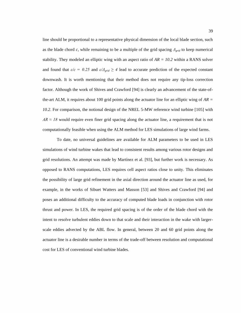
39

line should be proportional to a representative physical dimension of the local blade section, such

as the blade chord c, while remaining to be a multiple of the grid spacing Δgrid to keep numerical

stability. They modeled an elliptic wing with an aspect ratio of AR = 10.2 within a RANS solver

and found that ε/c = 0.25 and ε/Δgrid ≥ 4 lead to accurate prediction of the expected constant

downwash. It is worth mentioning that their method does not require any tip-loss correction

factor. Although the work of Shives and Crawford [94] is clearly an advancement of the state-of-

the-art ALM, it requires about 100 grid points along the actuator line for an elliptic wing of AR =

10.2. For comparison, the notional design of the NREL 5-MW reference wind turbine [105] with

AR ≈ 18 would require even finer grid spacing along the actuator line, a requirement that is not

computationally feasible when using the ALM method for LES simulations of large wind farms.

To date, no universal guidelines are available for ALM parameters to be used in LES

simulations of wind turbine wakes that lead to consistent results among various rotor designs and

grid resolutions. An attempt was made by Martínez et al. [93], but further work is necessary. As

opposed to RANS computations, LES requires cell aspect ratios close to unity. This eliminates

the possibility of large grid refinement in the axial direction around the actuator line as used, for

example, in the works of Sibuet Watters and Masson [53] and Shives and Crawford [94] and

poses an additional difficulty to the accuracy of computed blade loads in conjunction with rotor

thrust and power. In LES, the required grid spacing is of the order of the blade chord with the

intent to resolve turbulent eddies down to that scale and their interaction in the wake with larger-

scale eddies advected by the ABL flow. In general, between 20 and 60 grid points along the

actuator line is a desirable number in terms of the trade-off between resolution and computational

cost for LES of conventional wind turbine blades.

40

4.2 Overview of Work Presented in This Chapter

The subsequent sections in this chapter present the work on quantifying and improving

the capability of state-of-the-art ALM in predicting spanwise blade loads along with integrated

rotor thrust and power. All the simulations are performed with steady and uniform inflow only

and on two types of grid, i) LES-type grids with grid aspect ratio close to unity, and ii) stretched

grids (for a few cases). A rigorous study on assessing ALM accuracy through comparison against

available data, classical lifting-line solutions, and a blade-element momentum (BEM) method is

preformed. The sensitivity of computed sectional blade loads as well as integrated rotor thrust and

power on the major ALM parameters ε, Δgrid, and Δb is studied. An assessment of accuracy of the

state-of-the-art ALM with regards to the ALM parameters, primarilry ε, is performed by studying

an elliptically loaded wing with two different planforms, and the NREL Phase VI rotor under

parked and rotating conditions. Next, a new method is presented in which the Gaussian radius ε is

based on an equivalent elliptic blade planform of the same AR as the actual blade. The basic idea

of the new method was inspired by the work of Schrenk [106] used in the fixed-wing community

and leads to a set of universal criteria to be used for the ALM parameters on LES-type grids.

Next, available data for the NREL Phase VI rotor [107] and BEM results are used for quantitative

comparisons against results obtained by new ALM runs with various parameter settings.

Comparisons between the currently used settings and the proposed new criteria are performed for

the cases for which an accuracy assessment was performed. It is found that the new method for

the Gaussian radius ε and guidelines for the grid spacing Δgrid and actuator spacing Δb yield

improved and consistent predictions for sectional blade loads. Also, ALM simulations are

performed for the NREL 5-MW turbine using the new method and compared to BEM results and

other ALM approaches. It is again found that the new method in which the Gaussian radius ε is

determined by an equivalent elliptic blade planform gives consistent and improved predictions of

41

sectional blade loads. The chapter concludes with recommendations for users of the ALM on

LES-type grids.

4.3 Existing Actuator Line Modeling Approaches

This section describes the two types of existing actuator line modeling approaches, one

based on grid resolution (default) and the other based on the local chord along the blade span.

4.3.1 Grid-Based ALM

The default ALM developed by Sørensen and Shen [56] is based on the grid-resolution,

Δgrid, in the vicinity of the turbine (or lifting line). A common rule-of-thumb states that ε should

be chosen as small as possible, however a minimum threshold exists in order to avoid numerical

instabilities that occur when the radius of the body force applied to equation 3-8 is too small such

that it resembles a discontinuity. These instabilities appear as ―ringing‖ when the convection

term of the momentum equation is discretized using central differencing. Troldborg [62],

therefore, suggests a Gaussian spreading width (or radius), ε = 2*Δgrid, in order to maintain

numerical stability and to obtain good predictions of the rotor power. At each actuator point along

the span, the same ε is used, i.e. ε (r) = constant, and this is based on grid resolution only, i.e. ε (r)

= const*Δgrid. Any physical dimension such as blade chord is not considered. A detailed study of

the effect of the Gaussian width, ε, in conjunction with grid resolution has been performed by

Martínez et al. [93]. They found that at a given inflow wind speed and a given ε, the computed

rotor power converges as the grid is refined; however, as ε/Δgrid is varied from 2 to 10.5, the

predicted power increases by about 25%, which is significant. This shows the sensitivity of the

grid-based ALM.

42

4.3.2 Chord-Based ALM

It has only been recently that sectional blade inflow conditions have been considered in

the context of ALM accuracy in addition to computed rotor thrust and/or power. It is the local

induced flow at a section of blade that defines a blade section‘s angle of attack (AOA) and hence

local lift and drag forces. Shives and Crawford [94] performed RANS simulations of an elliptic

wing of AR = 10.2 and investigated how the Gaussian spreading width ε affects the computed

inflow, in particular the downwash, at the actuator line. They found that it is advantageous to

choose ε based on the local blade chord, c(r). It was found that ε/c = 0.25 is suitable to compute

the expected constant downwash distribution at an elliptically loaded lifting (or actuator) line at a

high accuracy and given ε/Δgrid ≥ 4. Though their work is very promising and suggests that ε

should be chosen relative to the actual blade planform, c(r), one can argue that the proposed

method breaks down for a rectangular wing that is twisted such that an elliptic lift distribution

with constant downwash is achieved. In this case, the ε/c = constant criterion results in a constant

Gaussian spreading width ε along the blade span, and the actual grid spacing Δgrid determines

what the value for ε/Δgrid will be.

An attempt to perform simulations similar to Shives and Crawford for the NREL Phase

VI rotor with cmin/R = 0.0707 at the blade tip would require a grid spacing of Δgrid/R = 1/226

assuming a LES-type grid with a cell aspect ratio of unity. There is no doubt that such a high grid

resolution along the actuator line is not feasible for ABL-LES simulations of large wind farms

using the ALM. However, Shives and Crawford also state that their criteria may be to some

extent specific to the solver used for the simulations. Allowing a larger cell aspect ratio in the

ABL-LES simulations around the actuator line in conjunction with higher values for ε/c, the

criteria suggested by Shives and Crawford may be relaxed.

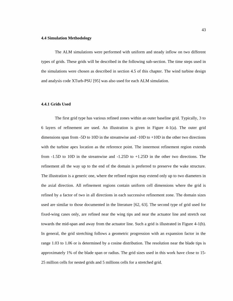
43

4.4 Simulation Methodology

The ALM simulations were performed with uniform and steady inflow on two different

types of grids. These grids will be described in the following sub-section. The time steps used in

the simulations were chosen as described in section 4.5 of this chapter. The wind turbine design

and analysis code XTurb-PSU [95] was also used for each ALM simulation.

4.4.1 Grids Used

The first grid type has various refined zones within an outer baseline grid. Typically, 3 to

6 layers of refinement are used. An illustration is given in Figure 4-1(a). The outer grid

dimensions span from -5D to 10D in the streamwise and -10D to +10D in the other two directions

with the turbine apex location as the reference point. The innermost refinement region extends

from -1.5D to 10D in the streamwise and -1.25D to +1.25D in the other two directions. The

refinement all the way up to the end of the domain is preferred to preserve the wake structure.

The illustration is a generic one, where the refined region may extend only up to two diameters in

the axial direction. All refinement regions contain uniform cell dimensions where the grid is

refined by a factor of two in all directions in each successive refinement zone. The domain sizes

used are similar to those documented in the literature [62, 63]. The second type of grid used for

fixed-wing cases only, are refined near the wing tips and near the actuator line and stretch out

towards the mid-span and away from the actuator line. Such a grid is illustrated in Figure 4-1(b).

In general, the grid stretching follows a geometric progression with an expansion factor in the

range 1.03 to 1.06 or is determined by a cosine distribution. The resolution near the blade tips is

approximately 1% of the blade span or radius. The grid sizes used in this work have close to 15-

25 million cells for nested grids and 5 millions cells for a stretched grid.

44

(a) Nested refined grid (wind turbine)

(b) Planes of the stretched grid (fixed wing)

Figure 4-1. Examples of grids used for actuator line simulations.

45

4.4.2 XTurb-PSU

XTurb-PSU is an in-house developed wind turbine design and performance prediction

code [95, 96]. XTurb-PSU uses either BEM theory based on NREL‘s AeroDyn code [97] or a

prescribed helicoidal vortex method (HVM) [98]. It also employs a stall delay model by Du and

Selig [99] rooted in NREL‘s AirfoilPrep worksheet [100]. The XTurb-PSU code is used in BEM

mode for rotating conditions reported in this work to produce reference results for quantitative

comparisons against the ALM with various spreading methods for the Gaussian radius ε. The

HVM module in XTurb-PSU has been used for analyzing wind turbines under parked conditions

and fixed wings in steady flow. This makes the XTurb-PSU code a flexible performance tool for

both the rotating and parked test cases considered in this work. However, XTurb-PSU lacks the

capability to model transient blade loads and turbulent inflow.

4.5 Accuracy Assessment of Actuator Line Method

In order to assess the accuracy of the present ALM, simulations were performed for the

the NREL Phase VI rotor, and two non-rotating wings both with an elliptical spanwise loading. A

grid dependence study was conducted for the NREL Phase VI rotor prior to the accuracy

assessment.

4.5.1 Grid-Dependence Study

Details of the three different grids used for the dependence study are presented in Table

4-1. Each grid has several layers (typically three or four) of refinement, as illustrated in Figure 4-

1(a). The smallest grid spacings near the blades are , , and in the three

coordinate directions, all nearly equal to the intended Δgrid. The Gaussian width, ε, was chosen

46

such that it is about twice the grid resolution in the vicinity of the turbine. The operating

conditions and the relevant simulation parameters for the NREL Phase VI rotor are presented in

Table 4-2. The simulations for the NREL Phase VI rotor under rotating and parked conditions

were performed using all three grids shown in Table 4-1 with the parameters shown in Table 4-2.

The simulations for the parked condition involved additional parameters presented in Table 4-3.

The ALM simulations for the rotating condition were performed with and without the Glauert

correction [101] for computed blade loads, while no Glauert correction was used for the parked

condition. The number of actuator points in each case was such that Δb Δgrid.

The results obtained using the three grids described above are presented in Figures 4-2

through 4-4. The Glauert correction was used for the CFD simulations for the rotating case.

Figures 4-2, 4-3, and 4-4 show the spanwise variation of AOA, normal force coefficient, , and

tangential force coeffient, , respectively. It can be observed that the results obtained using all

three grids agree quite well. The experimental results for and are also presented, and they

agree reasonably well with the computed results for the rotating case when the Glauert correction

is applied. However, the AOA does not show a consistent trend at the blade tip. This is because

the Glauert correction is applied only to the force coefficients and not to the actual flow field that

trails into the wake. For the parked case, the agreement is very good except at the root and tip.

The application of the Glauert correction within an ALM method remains an unsolved issue and

will be investigated further in the next section. The grid dependence study presented above

suggests that Grid 3 can be used for the analysis of sectional blade loads for the remaining test

cases for accuracy assessment.

47

Table 4-1. Details of the grids considered for NREL Phase VI rotor simulations.

Table 4-2. NREL Phase VI rotor - Geometric parameters and operating conditions.

NREL Phase VI Rotor

Rotor Radius, R ( ) 5.029

Wind Speed, ( ) 7.0

Rotor Speed (RPM) 72.0

Root Cutout, r/R 0.0859

Table 4-3. Simulation parameters for NREL Phase VI rotor under rotating and parked conditions.

NREL Phase VI Rotor Rotating Parked

Rated Wind Speed, (m/s) 7.0 20.1

Time Step, Δt (sec) 0.00174 0.00327

or (m) 0.0658 0.0658

Pitch (degrees) 3.0 81.859

48

(a) Rotating (Vwind = 7 m/s) (b) Parked (Vwind = 20.1 m/s)

Figure 4-2. Spanwise variation of angle of attack for NREL Phase VI rotor.


Figure 4-3. Spanwise variation of normal force coefficient for NREL Phase VI rotor.


Figure 4-4. Spanwise variation of tangential force coefficient for NREL Phase VI rotor.

49

4.5.2 NREL Phase VI Rotor, ε/Δgrid = constant

The simulations for the NREL Phase VI rotor using grid-based ALM (ε/Δgrid = constant)

under rotating and parked conditions were performed on Grid 3 described in section 4.5.1. It

should be noted that for grid-based ALM, Δb Δgrid, so ε/Δgrid and ε/Δb can be used

interchangeably.

4.5.2.1 Rotating Condition

Measured data for the sectional normal and tangential forces are available from NREL.

Following the convention used in the NREL Phase VI experiment [107], the normal force acts

orthogonal to the local chord line and towards the upper surface of the local airfoil section, while

the tangential force acts in the local chord direction and towards the local leading edge [107]. The

Prandtl/Glauert correction is applied locally to both the airfoil lift and drag coefficients. It has

been implemented in exactly the same manner as the F1 correction described in Shen et al. [103].

Figures 4-5 and 4-6 show the spanwise variation of normal and tangential force coefficients, Cn

and Ct respectively, for the NREL Phase VI rotor at a wind speed of 7 m/s, where the flow is

attached along the entire blade. A quantitative comparison with results obtained by XTurb-PSU

and measured NREL data is also shown. It is quite obvious that the ALM over-predicts AOA and

resultant blade loads near the root and tip.

Figure 4-7 shows the spanwise distribution of the local AOA, which is a good indicator

of how well the local inflow conditions at the actuator line are predicted. It can be seen that the

ALM over-predicts the local AOA towards the blade tips, which leads to the observed over-

prediction of normal and tangential force coefficients in Figures 4-5 and 4-6. Results obtained by

the Glauert/Prandtl correction in Figures 4-5 and 4-6 actually under-predict the force coefficients

50

considered when compared to NREL data and results obtained by XTurb-PSU. The

Glauert/Prandtl correction only affects the force coeffcients and hardly affects the AOA. The

ultimate goal is to not use it in the simulations because i) it should not be necessary in a computed

3-D flow field, and ii) there is no equivalent correction factor that can be used in non-rotating (or

parked) flow conditions.

Figure 4-5. Spanwise variation of normal force coefficient for NREL Phase VI rotor (Vwind =

7m/s), ALM parameters: ε/Δgrid = constant, Δgrid /R = 1/30, Δb /Δgrid = 1

Figure 4-6. Spanwise variation of tangential force coefficient for NREL Phase VI rotor (Vwind =

7m/s), ALM parameters: ε/Δgrid = constant, Δgrid /R = 1/30, Δb /Δgrid = 1

51

Figure 4-7. Spanwise variation of angle of attack for NREL Phase VI rotor (Vwind = 7m/s), ALM

parameters: ε/Δgrid = constant, Δgrid /R = 1/30, Δb /Δgrid = 1

A shortcoming of using a constant Gaussian radius ε along the span of the blade has been

identified above. The Glauert/Prandtl correction hardly affects the velocity field, and hence AOA,

along the span. The aerodynamic forces are the combined effect of force coeffients (affected by

Glauert correction) and velocity field (unaffected by Glauert correction). Therefore, it is worth

considering the aerodynamic forces along the span. Even though the trends are clear from the

above discussion, further assessment will be done with a slightly finer grid (Δgrid/R = 1/32) and

ε/Δgrid = 2, while still maintaining Δb /Δgrid = 1.

Figure 4-8 shows ALM-computed AOAs along the blade for various constant Gaussian

radii in comparison to results obtained by the XTurb-PSU code. Both the ALM and XTurb-PSU

code use the same sectional S809 airfoil data along the blade span in the respective computations.

Sectional lift and drag forces, which define the local blade force vector, (equation 3-9),

strictly depend on the computed local AOA. It is quite apparent that a constant Gaussian radius

complying with ε/Δgrid = constant leads to a noticeable overprediction of blade tip loads.

Furthermore, as ε/Δgrid is reduced, the AOA distribution is shifted towards the reference case of

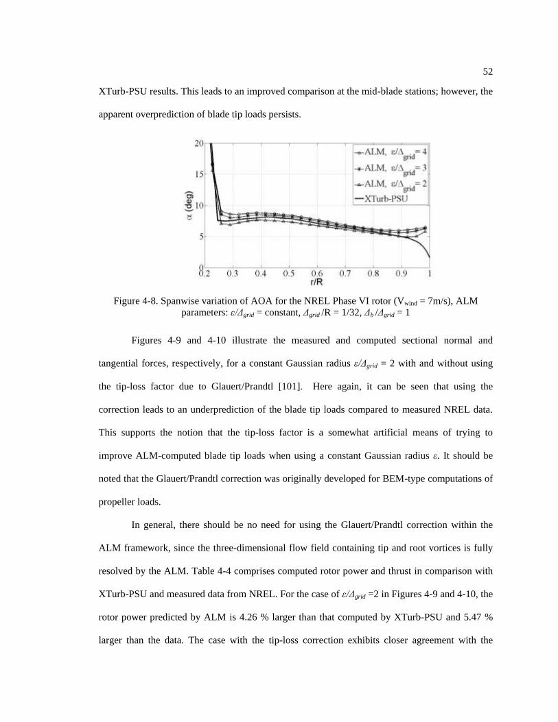
52

XTurb-PSU results. This leads to an improved comparison at the mid-blade stations; however, the

apparent overprediction of blade tip loads persists.

Figure 4-8. Spanwise variation of AOA for the NREL Phase VI rotor (Vwind = 7m/s), ALM

parameters: ε/Δgrid = constant, Δgrid /R = 1/32, Δb /Δgrid = 1

Figures 4-9 and 4-10 illustrate the measured and computed sectional normal and

tangential forces, respectively, for a constant Gaussian radius ε/Δgrid = 2 with and without using

the tip-loss factor due to Glauert/Prandtl [101]. Here again, it can be seen that using the

correction leads to an underprediction of the blade tip loads compared to measured NREL data.

This supports the notion that the tip-loss factor is a somewhat artificial means of trying to

improve ALM-computed blade tip loads when using a constant Gaussian radius ε. It should be

noted that the Glauert/Prandtl correction was originally developed for BEM-type computations of

propeller loads.

In general, there should be no need for using the Glauert/Prandtl correction within the

ALM framework, since the three-dimensional flow field containing tip and root vortices is fully

resolved by the ALM. Table 4-4 comprises computed rotor power and thrust in comparison with

XTurb-PSU and measured data from NREL. For the case of ε/Δgrid =2 in Figures 4-9 and 4-10, the

rotor power predicted by ALM is 4.26 % larger than that computed by XTurb-PSU and 5.47 %

larger than the data. The case with the tip-loss correction exhibits closer agreement with the

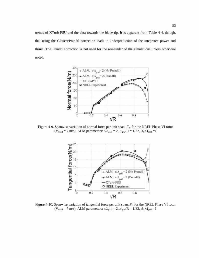
53

trends of XTurb-PSU and the data towards the blade tip. It is apparent from Table 4-4, though,

that using the Glauert/Prandtl correction leads to underprediction of the integrated power and

thrust. The Prandtl correction is not used for the remainder of the simulations unless otherwise

noted.

Figure 4-9. Spanwise variation of normal force per unit span, Fn, for the NREL Phase VI rotor

(Vwind = 7 m/s), ALM parameters: ε/Δgrid = 2, Δgrid/R = 1/32, Δb /Δgrid =1

Figure 4-10. Spanwise variation of tangential force per unit span, Ft, for the NREL Phase VI rotor

(Vwind = 7 m/s), ALM parameters: ε/Δgrid = 2, Δgrid/R = 1/32, Δb /Δgrid =1

54

Table 4-4. Rotor power and thrust - NREL Phase VI rotor (Vwind = 7 m/s), ALM parameters:

ε/Δgrid = constant, Δgrid /R = 1/32, Δb /Δgrid = 1.

NREL Phase VI Rotor Power (W) Thrust (N)

NREL Experiment 6,030 1,120

XTurb-PSU 6,100 1,240

ALM (ε/Δgrid = 4.0) 7,390 1,405

ALM (ε/Δgrid = 3.0) 7,100 1,380

ALM (ε/Δgrid = 2.0) 6,360 1,310

ALM (ε/Δgrid = 2.0, Prandtl factor) 5,520 1,090

4.5.2.2 Parked Condition

The simulations for the NREL Phase VI rotor under a parked condition (Vwind = 20.1 m/s,

pitch = 81.59 degrees) were performed using the parameters outlined in Table 4-3. Since the

blades are not moving in the parked state, the time step, Δt, was chosen such that the wind

traverses the same distance per time step as the blade tip does under rotating conditions.

Figures 4-11 and 4-12 show the spanwise variation of normal and tangential force

coefficients, Cn and Ct, respectively, for the NREL Phase VI rotor in a parked condition in

comparison with NREL data and results obtained by XTurb-PSU. Improved agreement is

observed when compared to the rotating case. Some discrepancy at the blade root and tip,

however, persists.

The same can be observed for the spanwise AOA distribution in Figure 4-13. Up to this

point, there are strong indications that the grid-based ALM does not predict accurately the flow

conditions and loads near the blade root and tip for a constant Gaussian spreading width ε for

both rotating and parked conditions. The exact reason for this is unclear at present, however one

can surmise that it must be related to the facts that the volumetric body-force spreading acts

beyond the geometric blade edges and that the strong force gradients near the blade tip, for

example, are alleviated by the force spreading at more inboard stations (e.g. 90% R) that leads to

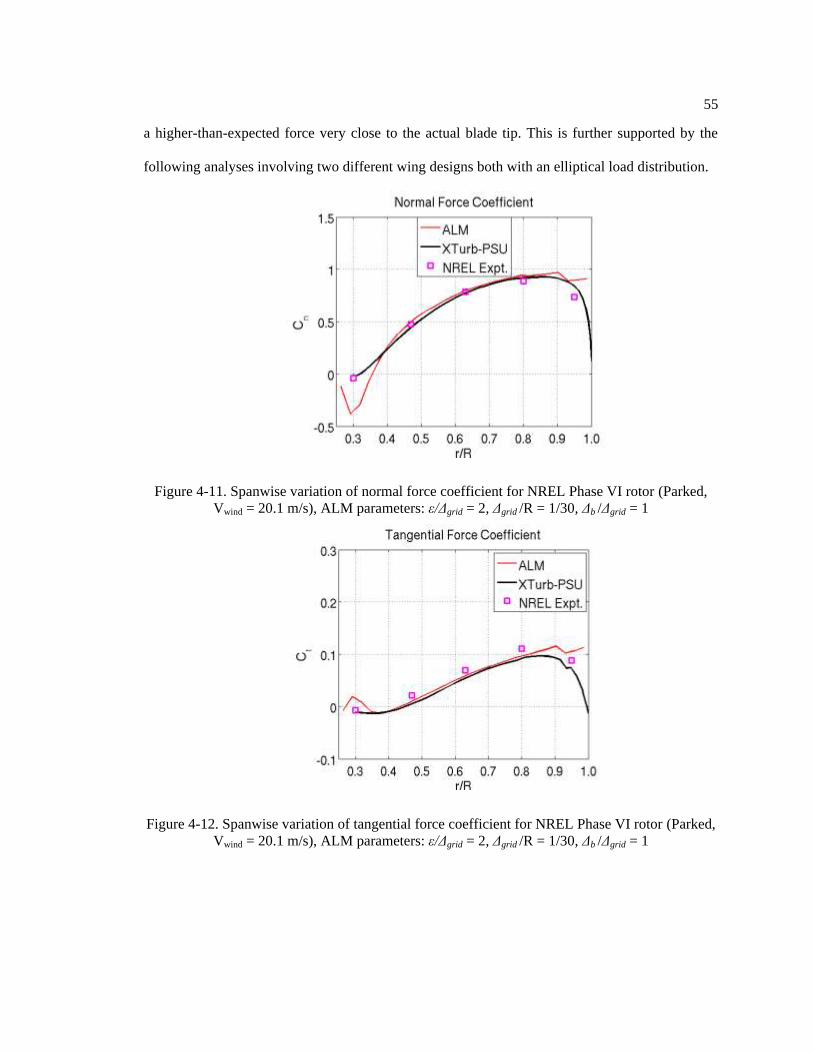
55

a higher-than-expected force very close to the actual blade tip. This is further supported by the

following analyses involving two different wing designs both with an elliptical load distribution.

Figure 4-11. Spanwise variation of normal force coefficient for NREL Phase VI rotor (Parked,

Vwind = 20.1 m/s), ALM parameters: ε/Δgrid = 2, Δgrid /R = 1/30, Δb /Δgrid = 1

Figure 4-12. Spanwise variation of tangential force coefficient for NREL Phase VI rotor (Parked,

Vwind = 20.1 m/s), ALM parameters: ε/Δgrid = 2, Δgrid /R = 1/30, Δb /Δgrid = 1

56

Figure 4-13. Spanwise variation of angle of attack for NREL Phase VI rotor (Parked, Vwind = 20.1

m/s), ALM parameters: ε/Δgrid = 2, Δgrid /R = 1/30, Δb /Δgrid = 1

4.5.3 Elliptically Loaded Wing, ε/Δgrid = constant

The elliptically loaded wing is a classical optimal case in applied aerodynamics. In order

to test the grid-based ALM, a wing with an elliptic planform was designed that has the same wing

area (3.066 m2) and aspect ratio (8.249) as the NREL Phase VI rotor blade whose near-root

cylindrical section (r/R < 0.25) is replaced by an extrapolation of the aerodynamic part. An

illustration is given in Figure 4-14. In this case, a grid was used such that Δgrid/R = 1/37, requiring

the number of actuator points along the actuator line to be 37, so that Δb Δgrid can be

maintained. The Gaussian spreading width ε was chosen to be about four times the actuator

spacing Δb as a baseline test case. The wing is exclusively equipped with the S809 airfoil. The

geometric AOA was set to be 8°, leading to a mid-span circulation (Г0) of 6.6816 (m2/s) and an

induced AOA (αi) of 1.8936° according to finite-wing theory. Two wings were designed with one

being untwisted and having an elliptic planform (or chord) distribution, while the second one has

a rectangular planform (constant chord) and is twisted such that it produces an elliptic lift

57

distribution at a geometric AOA of 8°. Table 4-5 summarizes some of the geometric and

simulation parameters.

Figure 4-14. Wing with elliptic planform designed for analysis

Table 4-5. Details of the wing designs with elliptical load distribution

Planform Elliptic Rectangular

Span (m) 5.029 5.029

Area (m2) 3.066 3.066

Aspect Ratio 8.249 8.249

Mid-Chord (m) 0.7763 0.6096

Wind Speed, Vwind (m/s) 20.1 20.1

Time Step, Δt (sec) 0.0033 0.0033

Vwind Δt (m) 0.0658 0.0658

Actuator Width, Δb/R 1/37 1/37

Twist (degrees) 0 0 to 8

4.5.3.1 Elliptic Planform

Classical lifting-line theory thus suggests a constant effective AOA of 6.1064° along the

span of the wing described above. Figure 4-15 shows the AOA, and Figures 4-16 and 4-17 show

the normal and tangential force coefficients, Cn and Ct, respectively, for the designed elliptic-

wing planform. The results from XTurb-PSU match well with the theory as expected from a

58

lifting-line model. The ALM predictions exhibit quite large discrepancies when compared to

XTurb-PSU and the theoretical results. It can also be observed that as ε decreases the predicted

AOA decreases, and the strong deviation from the theoretical results near the wing tips occurs

over a smaller portion of the wing.

Figure 4-15. Spanwise variation of angle of attack for elliptically loaded wing (Elliptic planform,

Vwind = 20.1 m/s), ALM parameters: ε/Δgrid = const, Δgrid /R = 1/37, Δb /Δgrid = 1

Figure 4-16. Spanwise variation of normal force coefficient for elliptically loaded wing (Elliptic

planform, Vwind = 20.1 m/s), ALM parameters: ε/Δgrid = const, Δgrid /R = 1/37, Δb /Δgrid = 1

59

Figure 4-17. Spanwise variation of tangential force coefficient for elliptically loaded wing

(Elliptic planform, Vwind = 20.1 m/s), ALM parameters: ε/Δgrid = const, Δgrid /R = 1/37, Δb /Δgrid = 1

4.5.3.2 Rectangular Planform

The blade twist of the rectangular wing was designed with the exact same elliptic

circulation distribution as for the wing with elliptic planform described above. Figure 4-18 shows

the AOA, and Figures 4-19 and 4-20 show the normal and tangential force coefficients, Cn and Ct

respectively, for the wing with rectangular planform and elliptical loading. The results from

XTurb-PSU match again well with the theory with small deviations.. The ALM predictions of

AOA are close to the theory and XTurb-PSU results except at the wing tips. The force

coefficients predicted by ALM exhibit some deviation compared to those computed by XTurb-

PSU.

The previous observation that AOA and blade tip loads are over-predicted for ε/Δgrid =

constant holds true for both wing designs.

60

Figure 4-18. Spanwise variation of angle of attack for elliptically loaded wing (Rectangular

planform, Vwind = 20.1 m/s), ALM parameters: ε/Δgrid = 4.01, Δgrid /R = 1/37, Δb /Δgrid = 1


(Rectangular planform, Vwind = 20.1 m/s), ALM parameters: ε/Δgrid = 4.01, Δgrid /R = 1/37, Δb /Δgrid

= 1

61


(Rectangular planform, Vwind = 20.1 m/s), ALM parameters: ε/Δgrid = 4.01, Δgrid /R = 1/37, Δb /Δgrid

= 1

4.5.4 NREL Phase VI Rotor, ε/c = constant

In the previous two sub-sections, the accuracy of grid-based ALM (ε/Δgrid = constant) was

assessed for the NREL Phase VI rotor under rotating and parked conditions and for an elliptically

loaded wing with elliptic and rectangular planforms. It was observed that AOA and blade tip

loads are over-predicted for all these test cases.

In this sub-section, the accuracy of the chord-based ALM (ε/c = constant) will be

investigated along the lines of the work of Shives and Crawford [94]. This is done by choosing a

grid resolution of Δgrid/R = 1/37, far smaller than that used by Shives and Crawford for an elliptic

wing. The criterion suggested byTroldborg [62] and the observation above for the grid-based

ALM suggests that a Gaussian spreading width, ε, of 3 to 4 times the grid resolution would be a

good candidate for testing. Since the logic of using chord-based ALM is rooted in the fact that the

effect of the actual blade geometry on the flow field should be commensurate with the geometry

itself, the chosen Gaussian spreading width should correspond to the maximum chord along the

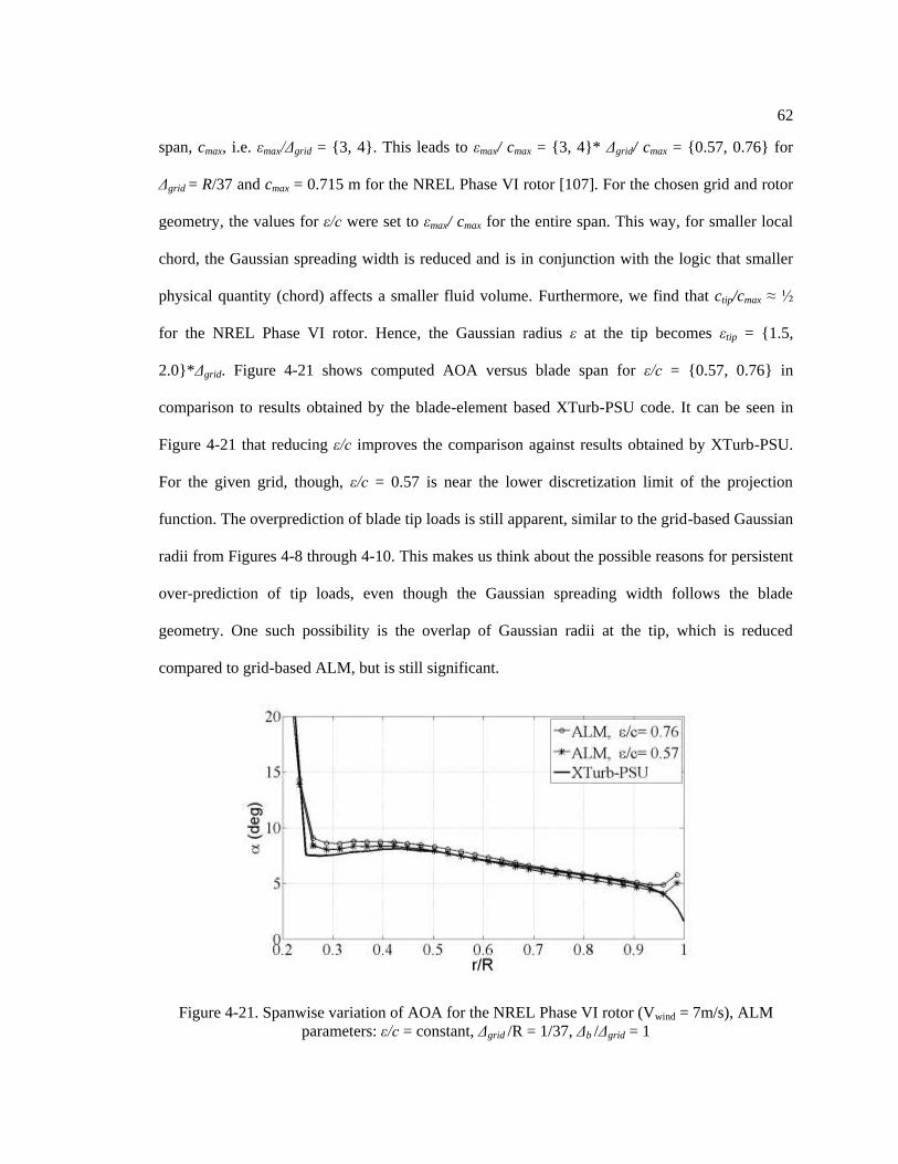
62

span, cmax, i.e. εmax/Δgrid = {3, 4}. This leads to εmax/ cmax = {3, 4}* Δgrid/ cmax = {0.57, 0.76} for

Δgrid = R/37 and cmax = 0.715 m for the NREL Phase VI rotor [107]. For the chosen grid and rotor

geometry, the values for ε/c were set to εmax/ cmax for the entire span. This way, for smaller local

chord, the Gaussian spreading width is reduced and is in conjunction with the logic that smaller

physical quantity (chord) affects a smaller fluid volume. Furthermore, we find that ctip/cmax ≈ ½

for the NREL Phase VI rotor. Hence, the Gaussian radius ε at the tip becomes εtip = {1.5,

2.0}*Δgrid. Figure 4-21 shows computed AOA versus blade span for ε/c = {0.57, 0.76} in

comparison to results obtained by the blade-element based XTurb-PSU code. It can be seen in

Figure 4-21 that reducing ε/c improves the comparison against results obtained by XTurb-PSU.

For the given grid, though, ε/c = 0.57 is near the lower discretization limit of the projection

function. The overprediction of blade tip loads is still apparent, similar to the grid-based Gaussian

radii from Figures 4-8 through 4-10. This makes us think about the possible reasons for persistent

over-prediction of tip loads, even though the Gaussian spreading width follows the blade

geometry. One such possibility is the overlap of Gaussian radii at the tip, which is reduced

compared to grid-based ALM, but is still significant.


parameters: ε/c = constant, Δgrid /R = 1/37, Δb /Δgrid = 1

63


(Vwind = 7m/s), ALM parameters: ε/c = 0.57, Δgrid/R = 1/37, Δb /Δgrid = constant


(Vwind = 7m/s), ALM parameters: ε/c = 0.57, Δgrid/R = 1/37, Δb /Δgrid = constant

In the following, the actuator spacing Δb/Δgrid is varied with the idea of reducing the

overlap regions of the volumetric body-force distribution around an actuator point. Figures 4-22

and 4-23 show the normal and tangential force coefficients, Cn and Ct, respectively. They reveal

that increasing the actuator spacing has a small, though positive, effect on predicting the blade tip

loads. The reason for this observation is believed to be related to the strength of the trailing

vorticity emanating from the actuator line between the two actuator points closest to the blade tip.

64

If the Gaussian radius ε is too large compared to the actuator spacing Δb, then adjacent

overlapping force distributions may lower the strength of the trailing vorticity and hence induce

less downwash at the actuator line that leads to the observed overprediction in the AOA close to

the blade tip. For εtip = 1.5 Δgrid in Figures 4-22 and 4-23, the Gaussian has reduced to 64 % of its

peak strength at the adjacent inboard actuator point for Δb/Δgrid = 1.0 (ε = 1.5 Δgrid and |r| = 1.0

Δgrid in equation 3-10, making the Gaussian decay to at the adjacent inboard actuator

point). Similarly, the Gaussian reduces to 37 % and 24 %, respectively, for Δb/Δgrid = 1.5 and 1.8.

As noted earlier, a small improvement can be seen in the tip-load prediction in Figures 4-22 and

4-23; however, one has to be aware that Δb/Δgrid = 1.8 results in Δb/R ≈ 1/20 (or 20 actuator points

along the actuator line), which can be considered a minimum requirement for the number of blade

elements along an actuator (or lifting) line.

Computed rotor power and thrust are summarized in Table 4-6. Maximum discrepancies

between results obtained by XTurb-PSU and ALM amount to 1.8% for the rotor power and 4.0%

for the rotor thrust for the ALM simulation with Δb /Δgrid = 1.5. Figures 4-22 and 4-23 support,

however, that the close agreement between XTurb-PSU and ALM results is an artifact of

cancelling spanwise under- and overprediction of blade loads.

Table 4-6. Rotor power and thrust - NREL Phase VI rotor (Vwind = 7 m/s), ALM parameters: ε/c =

0.57, Δgrid /R = 1/37, Δb /Δgrid = constant



XTurb-PSU 6,100 1,240

ALM (Δb /Δgrid = 1.0) 6,170 1,280

ALM (Δb /Δgrid = 1.5) 6,210 1,290

ALM (Δb /Δgrid = 1.8) 6,105 1,275

65

4.6 Proposed Guidelines for Gaussian Spreading

As mentioned in section 4.1, the main parameters that affect the volumetric distribution

of body forces Fp around the actuator line are the Gaussian radius ε, the grid spacing Δgrid in the

vicinity of the actuator line, and the distance between actuator points Δb. To date, the main

lessons learned about the choice of ALM parameters (through studies conducted by other

researchers and the assessment conducted in section 4.5) are:

i) the Gaussian radius ε should be small, to resemble a line, but must be large enough

relative to the grid to maintain numerical stability [63];

ii) depending on the choice of grid resolution and a spanwise constant value of Gaussian

radius, the predicted power may vary substantially [93]; and

iii) a blade-conforming ε/c = constant yields improved results of the computed inflow

distribution along an elliptic wing on stretched RANS-type grids [94].

In summary, the state-of-the-art in ALM suggests either a grid-based [63] or a chord-

based [94] Gaussian radius ε. In the following, a set of guidelines for choosing ALM parameters

towards a consistent body-force representation on LES-type grids is presented. As a first step,

some requirements and bounds for ALM parameters on LES-type grids are stated:

i) A relative grid spacing is approximately limited between Δgrid/R = [1/30, 1/60] and is

uniform along the actuator line to be both accurate and computationally feasible for

using the ALM to model large wind farms using LES.

ii) The relative spacing between actuator points satisfies Δb/R ≤ 1/20 such that rotor thrust

and power are computed accurately via integration over the actuator points along the

blade radius (or span), a guideline used in general for BEM methods.

iii) It is hypothesized that an elliptic Gaussian radius ε along the actuator line complies

with a first-order representation of a general blade loading. This hypothesis is the result

66

of a simple thought experiment that a chord based ε/c = constant criterion is equivalent

to a grid-based ε/Δgrid = constant Gaussian radius if the blade has a rectangular

planform. However, the blade may be appropriately twisted such that it achieves an

elliptic blade loading (as described in section 4.5.3), in which case the advantage of the

chord-based ε/c = constant criterion no longer applies.

The basic idea for the proposed guidelines was inspired by the ―Schrenk Approximation‖

[106] used in the fixed-wing community to estimate the wing loading distribution during the

aircraft design process. Here Schrenk‘s methodology is not followed exactly, but it is

hypothesized that the Gaussian radius ε should be chosen based on an elliptic blade planform of

the same aspect ratio as the actual blade, thus representing the first mode of the Fourier-series

solution of a general blade loading. A methodology for finding the ALM parameters ε, Δgrid, and

Δb is described below:

1. Determine the blade aspect ratio, AR

AR

∫

(4-1)

where R is the blade radius (or span ranging from –R/2 to R/2) and is the average blade

chord.

2. Find an ―equivalent‖ elliptic planform with the same AR

∗ √ (

)

(4-2)

3. Discretize the ―equivalent‖ ellipse for given Δgrid /R ≤ 1/30.

Set minimum discretization levels as:

a. nmin*Δgrid ; use nmin = 1 as a minimum discretization

threshold on any given grid. (4-3)

67

nmin need not be an integer.

nmin= 0 leads to numerical instabilities [108].

b. nmaxΔgrid ; The value for nmax is determined from

(4-4)

so that blade force is projected onto about 3 to 4 cells in the center of the ellipse if there

are about 30 cells along the blade span.

Complying with Δgrid /R ≤ 1/30, this results in nmax 3 and leads to a consistent

representation of the equivalent elliptic planform with grid refinement along the actuator line. nmax

need not be an integer.

Using Eqs. (4-1), (4-2), and (4-4), postulate that

∗ (

) constant (4-5)

while satisfying the minimum threshold of as shown in Figure 4-

24.

4. Actuator spacing, Δb /Δgrid

It is recommended that the actuator spacing be chosen approximately such that

(4-6)

As the actuator line is discretized into segments and actuator points that lie in the middle

of the segments, there are no actuator points coincident with the tip and root. Eq. (4-5) in

conjunction with εR/2 =Δgrid from Eq. (4-3) thus ensures that, when the Gaussian in equation 3-10

is used to project the actuator point force at the point adjacent to the blade tip and that adjacent to

the root, the projected force at the actual tip and root is only 10% of its peak value at the adjacent

actuator points. This assures that the body force does not extend appreciably beyond the location

68

of the blade tip and root due to force projection with a three-dimensional Gaussian. For the

coarsest grid spacing of Δgrid//R = 1/30, this results in Δb/R = 1/20, which represents a minimum

for blade-element integration.

Figure 4-24. Equivalent elliptic distribution of Gaussian radius, ε

Here the equivalent blade ellipse that defines the Gaussian radius ε(r) is shown on –R/2 ≤

r ≤ +R/2 for demonstration purposes only. For the actual computations of rotating blades and

reporting the blade loads, the equivalent ellipse is shifted such that 0 ≤ r ≤ +R in the code.

(a) NREL Phase VI rotor (b) NREL 5-MW turbine

Figure 4-25. Examples of the ‗equivalent‘ elliptic planform to define the Gaussian radius, ε

69

Thus, for a given blade planform and grid that satisfy Δgrid /R ≤ 1/30, Eqs. (4-1)–(4-6)

describe a general methodology for determining the most relevant ALM parameters, i.e., the

Gaussian radius ε, the grid spacing Δgrid, and the actuator spacing Δb. Figure 4-25 shows the

―equivalent‖ elliptic planform c* for the NREL Phase VI rotor blade and the NREL 5-MW

turbine blade. It is important to note that the equivalent elliptic planform c* is used solely for the

purpose of defining the Gaussian radius ε along the blade span; the actual blade forces are

computed using the actual blade chord distribution c.

4.7 Simulations Using Proposed Guidelines for Elliptic Gaussian Spreading

In this section, the new method described in section 4.6 for an elliptic Gaussian spreading

width ε is tested for the NREL Phase VI rotor under rotating and parked conditions and for an

elliptic wing. The guidelines presented in the previous section are then established for the NREL

Phase VI rotor under rotating condition. Finally, these guidelines are applied to the NREL 5-MW

turbine.

4.7.1 Preliminary Test for the NREL Phase VI Rotor, ε/c* = constant

The NREL Phase VI rotor blade has an aspect ratio (AR) of 10.455 as shown in Figure 4-

25(a). The ε/c*criterion in Equation (4-5) for the fictitious elliptic planform c* can be computed

for a chosen grid resolution and a user-specified nmax. The test cases for the proposed method

were performed on a grid with resolution Δgrid /R = 1/30 or Δgrid = 0.175 m. The values for nmax

were {3, 4} and those for nmin were {0, 1, 2}. Table 4-7 comprises the parameters associated with

the test cases. For comparison with the results for the grid-based and chord-based ALM, the

relevant parameters are also presented. The same set of parameters has been used for both

70

rotating and parked conditions. The integrated values of thrust and power, after the solutions

become stationary, have also been documented for each of these cases for the rotating condition

and are presented in Table 4-7.

Table 4-7. Parameters for constant, chord-based, and elliptic Gaussian spreading for NREL Phase

VI rotor, ALM parameters: Δgrid /R = 1/30, Δb /Δgrid = 1

ε - Method Fictitious

Chord,

(m)

ε (m)

ε/c

or

ε/c*

εmin /Δgrid

or

εtip /Δgrid

Integrated

Thrust

(N)

Integrated

Power

(W)

ε/Δgrid =

const

NA NA 0.7025

(4* Δgrid)

≠

const.

4 1450 7950

ε/c =

const

NA 4 ≠ const. 1.11 1 1425 7640

ε/c* =

const

0.6124 4 ≠ const. 1.11 2 1415 7545

0.6124 4 ≠ const. 1.11 1 1395 7350

0.6124 4 ≠ const. 1.11 0 1390 7340

0.6124 3 ≠ const. 0.83 1 1365 6970

4.7.1.1 Rotating Condition

The results obtained, using the method described in section 4.6 for an elliptic Gaussian

spreading width ε, are presented below for the NREL Phase VI rotor under rotating conditions.

The operating conditions are the same as for the accuracy assessment, as presented in Table 4-2.

Figures 4-26, 4-27 and 4-28 show the spanwise variation of AOA, Cn, and Ct respectively. It can

be observed that compared to the case of ε/Δgrid = constant, ε/c = constant (with actual planform)

produces slightly better results. However, it is the ε/c* = constant case that produces substantially

better results, particularly for the tip loads. It is worth noting that the Glauert/Prandtl correction is

not needed to obtain improved results for the blade tip loads. Comparing the various cases for the

proposed methods, it appears that nmax = 3 and nmin = 1 work quite well for the rotating case.

Apart from the sectional loads, the integrated thrust and power were also analyzed. It can

be noted from Table 4-7 that the new method alleviates the over-prediction of thrust and power.

The integrated thrust and power for nmax = 3 and nmin = 1 are 1365 N and 6970 W, respectively.

71

These values are much closer to the measured data, as listed in Table 4-4, compared to when a

constant ε/Δgrid is used, for the chosen grid resolution. It can be noted that the intergrated

power and thrust presented in Table 4-4 and Table 4-7 are for Δgrid /R = 1/32 and Δgrid /R = 1/30.

This also shows the dependence of integrated quantities on grid resolution for grid-based ALM

and calls for a more general approach, which alleviates this problem and is consistent across grid

resolutions. This work is presented in sub-section 4.7.3.

Figure 4-26. Spanwise variation of angle of attack for NREL Phase VI rotor (Vwind = 7m/s), ALM

parameters: Δgrid /R = 1/30, Δb /Δgrid = 1

72

Figure 4-27. Spanwise variation of normal force coefficient for NREL Phase VI rotor (Vwind =

7m/s), ALM parameters: Δgrid /R = 1/30, Δb /Δgrid = 1

73

Figure 4-28. Spanwise variation of tangential force coefficient for NREL Phase VI rotor (Vwind =

7m/s), ALM parameters: Δgrid /R = 1/30, Δb /Δgrid = 1

4.7.1.2 Parked Condition

The results for the NREL Phase VI rotor under parked conditions are presented below.

Figures 4-29, 4-30 and 4-31 show the spanwise variation of AOA, Cn, and Ct respectively. The

observations here are similar to those made for the rotating case. It can be noticed that the

proposed method produces improved results and that nmax = 3 and nmin = 1 work again well for the

parked case.

74

Figure 4-29. Spanwise variation of angle of attack for NREL Phase VI rotor (Parked, Vwind = 20.1

m/s), ALM parameters: Δgrid /R = 1/30, Δb /Δgrid = 1

Figure 4-30. Spanwise variation of normal force coefficient for NREL Phase VI rotor (Parked,

Vwind = 20.1 m/s), ALM parameters: Δgrid /R = 1/30, Δb /Δgrid = 1

75

Figure 4-31. Spanwise variation of tangential force coefficient for NREL Phase VI rotor (Parked,

Vwind = 20.1 m/s), ALM parameters: Δgrid /R = 1/30, Δb /Δgrid = 1

4.7.2 Preliminary Test for Elliptically Loaded Wing, ε/c* = constant

Having observed that the proposed method in section 4.6 for an elliptic Gaussian

spreading width ε shows improved results for the NREL Phase VI rotor, the classical

aerodynamics problem of an elliptically loaded wing was studied with the newly proposed

spreading method. Here, only the elliptic planform is considered as the rectangular planform of

the same AR results in the same fictitious elliptic planform c*. The criterion in Equation (4-5) for

the fictitious elliptic planform c* can be computed in the same manner as for the NREL Phase VI

76

rotor. Table 4-8 comprises the parameters associated with the test cases. The test cases were

performed on a grid with resolution Δgrid /R = 1/37 or Δgrid = 0.135 m.


elliptically loaded wing (elliptic planform, uniform grid), ALM parameters: Δgrid /R = 1/37, Δb

/Δgrid = 1


Chord,

(m)

ε (m)

ε/c

or

ε/c*

εmin /Δgrid

or

εtip /Δgrid

ε/Δgrid =

const

NA NA 0.5026

(4* Δgrid)

≠

const.

4

ε/c* =

const

0.7762 4 ≠ const. 0.5761 2

0.7762 4 ≠ const. 0.5761 1

0.7762 4 ≠ const. 0.5761 0

0.7762 3 ≠ const. 0.4321 1

Figures 4-32, 4-33 and 4-34 show the spanwise variation of AOA, Cn, and Ct,

respectively, obtained on a uniform grid described in section 4.4. It can be observed that,

compared to the case of ε/Δgrid = constant, the cases with ε/c* = constant show an under-

prediction of the blade tip loads except for one case. Comparing the various cases for the

proposed method, it appears that nmax = 4 and nmin = 1 work quite well for the wing. It can also be

seen that nmax = 4 and nmin = 0 leads to some instability.


uniform grid, Vwind = 20.1 m/s), ALM parameters: ε/c* = const, Δgrid /R = 1/37, Δb /Δgrid = 1

77


planform, uniform grid, Vwind = 20.1 m/s), ALM parameters: ε/c* = const, Δgrid /R = 1/37, Δb /Δgrid

= 1


(Elliptic planform, uniform grid, Vwind = 20.1 m/s), ALM parameters: ε/c* = const, Δgrid /R = 1/37,

Δb /Δgrid = 1

Figures 4-35, 4-36 and 4-37 show the spanwise variation of AOA, Cn, and Ct,

respectively, for the elliptic wing using a stretched grid (as shown in Figure 4-1(b)). The grid

used had the smallest resolution of 1% of span (0.05029 m) with the refined region around the

actuator line and near the tips extending over 20% span. An expansion factor of 1.05 was used.

The resulting radial spacing was 0.1242 m at the mid-span. Table 4-9 comprises the parameters

78

associated with the test cases for the stretched grid. Considering the resolutions at the tip as well

as mid-span, the ε/c* criterion in Equation (4-5) was computed with nmax = 4 and nmin = 1. The

cases for ε/Δgrid = constant were also considered for comparison. The Gaussian spreading width ε

was chosen such that ε/c0 was the same as ε/c* from above for each of the two grid resolutions

considered. Comparing the various cases for the proposed method, it appears that nmax = 4 and

nmin = 1 along with the ε/c* criterion based on the grid resolution at the mid-span produces the

best result. Thus, it can be concluded that grid stretching has a positive effect on the computed

inflow distribution. However, it should be noted that a nested grid is easier to use and has been

used everywhere else.


elliptically loaded wing (elliptic planform, stretched grid)


Chord,

(m)

Grid Resolution,

Δgrid (m)

ε (m)

ε/c

or

ε/c*

εmin /Δgrid

or

εtip /Δgrid

ε/Δgrid =

const

NA 0.05029 NA NA 0.2011 ≠ const. 4

NA 0.12420 NA NA 0.4968 ≠ const. 4

ε/c* =

const

0.7762 0.05029 4 1 ≠ const 0.2591 1

0.7762 0.12420 4 1 ≠ const 0.6400 1


stretched grid, Vwind = 20.1 m/s), ALM parameters: ε/c* = const, Δgrid /R = 1/37, Δb /Δgrid = 1

79


planform, stretched grid, Vwind = 20.1 m/s), ALM parameters: ε/c* = const, Δgrid /R = 1/37, Δb /Δgrid

= 1


(Elliptic planform, stretched grid, Vwind = 20.1 m/s), ALM parameters: ε/c* = const, Δgrid /R =

1/37, Δb /Δgrid = 1

4.7.3 Establishing Guidelines Using Simulations for the NREL Phase VI Rotor, ε/c* =

constant

In this sub-section, it is demonstrated that the proposed method in section 4.6 for

determining the ALM parameters ε, Δgrid, and Δb leads to improved and consistent results for

80

various computational grids and hence the guidelines are established. Figure 4-38 shows that an

elliptic Gaussian radius ε determined by the guidelines in section 4.6 results in AOA prediction

very comparable to the XTurb-PSU results. For a standard actuator spacing of Δb/Δgrid = 1.0,

however, the AOA at the blade tip is still overpredicted in comparison to XTurb-PSU. Increasing

Δb/Δgrid for εtip = εR/2 = Δgrid according to Eq. (4-3), the Gaussian in equation3-10 reduces to 0.21

(Δb/Δgrid = 1.25) and 0.11 (Δb/Δgrid = 1.50) of its peak value at the adjacent actuator point, and

eliminates the overprediction of AOA at the blade tip. It is apparent in Figure 4-38 that the elliptic

Gaussian radius ε governed by Eq. (4-5) for nmax = 3 results in an improved AOA prediction

compared to a grid-based or chord-based Gaussian radius.


parameters: ε/c* = 0.67, Δgrid /R = 1/37, Δb /Δgrid = constant

Next, it is shown that the general guidelines for ALM parameters described in section 4.6

predict consistent tip loads for various grid spacings Δgrid/R. Figures 4-39 and 4-40 show

computed sectional normal and tangential forces respectively, using the general guidelines for

ALM parameters defined in section 4.6 in comparison to the results computed by XTurb-PSU and

measured NREL data. It can be seen that consistent predictions are obtained when following the

general guidelines for the ALM parameters barring some load overprediction for all grids. For all

cases, εtip = εR/2 = Δgrid was used according to Eq. (4-3). For a reference grid of Δgrid/R = 1/37, nmax

81

= 3 was chosen, so that nmax Δgrid/R = 0.081 satisfies Eq. (4-4). As the grid spacing Δgrid/R is

refined, nmax is increased accordingly. Equation (4-5) hence results in ε/c* = 0.67 for a blade

aspect ratio of AR = 10.54. Furthermore, the time step Δt is reduced with grid refinement such

that the actuator line never traverses more than one grid cell per time step.


(Vwind = 7 m/s), ALM parameters: ε/c* = 0.67, Δgrid/R = constant, Δb /Δgrid = 1.5



In Figures 4-39 and 4-40, computed ALM results are very close to those obtained by

XTurb-PSU. In particular, the blade tip loads show improved agreement compared to a grid-

based or chord-based Gaussian radius, ε. There is still some apparent discrepancy between

82

computed and measured NREL data. At this stage, this is attributed to some inaccuracy in the

airfoil tables used for the ALM and XTurb-PSU computations. The airfoil tables for the S809

airfoil were obtained exclusively from the computer program XFOIL at various Reynolds

numbers and without any modifications to the built-in transition criterion within XFOIL. The

authors had decided not to use experimental data because previous work [109] had shown

apparent differences in measured S809 airfoil characteristics obtained in different facilities that

are not easy to assess. It was found, though [109], that XFOIL is capable of predicting the S809

airfoil characteristics very well within the experimental data range. Furthermore, no corrections

that account for blade rotation and three-dimensionality [99] were added to the airfoil tables in

order not to introduce additional empiricism that would distract from the main objective of this

work. It is apparent from the obtained ALM results that the proposed general guidelines show

improved comparison to computed XTurb-PSU and measured NREL data than those obtained

with a grid-based or chord-based Gaussian radius ε.

Although the load distributions in Figures 4-39 and 4-40 are quite consistent, integrated

rotor power and thrust in Table 4-10 seem to have not yet reached a converged state with respect

to grid refinement. For the ALM simulation with Δgrid/R = 1/64, the rotor power computed by

ALM is 8.4% higher and the rotor thrust 6.0% higher compared to results obtained by XTurb-

PSU. For the ALM simulations in Figures 4-39 and 4-40 and Table 4-10, nmax was scaled

according to Eq. (4-4) as the grid was refined. However, nmin = 1 was kept constant for all ALM

runs using Eq. (4-3) of the general guidelines as a minimum discretization level on a given grid.

Hence, the Gaussian radius ε has a slightly different distribution near the blade tips for each case.

It was therefore investigated whether scaling nmin according to nmax, i.e., having exactly the same

physical ε(r) between grids, would affect integrated rotor power and thrust. The corresponding

results in Table 4-10 for nmin = 1.2 on the grid with Δgrid /R = 1/45 and nmin = 1.7 on the grid with

Δgrid /R = 1/64 show in comparison to their counterparts on the same grid with nmin = 1 that the

83

effect is only on the order of one percent. This actually supports the use of Eq. (4-3) with nmin = 1

on any given grid. It is worth mentioning in this context that a previous study [93] has shown a

similar trend in ALM computed power with grid refinement where it was found that the

computed rotor power is converged to within approximately two percent for grids finer than

Δgrid/R = 1/64. The computational grid was therefore not refined beyond this resolution.

Table 4-10. Rotor power and thrust - NREL Phase VI rotor (Vwind = 7 m/s), ALM parameters: ε/c*

= 0.67, Δgrid /R = constant, Δb /Δgrid = 1.5.



XTurb-PSU 6,100 1,240

ALM (Δgrid /R = 1/37) 6,210 1,280

ALM (Δgrid /R = 1/45) 6,310 1,290

ALM (Δgrid /R = 1/64) 6,615 1,315

ALM (Δgrid /R = 1/45, nmin = 1.2) 6,340 1,300

ALM (Δgrid /R = 1/64, nmin = 1.7) 6,570 1,325

Figure 4-41 and 4-42 present the local AOA α and the square of the local velocity

magnitude V2mag respectively, both of which contribute directly to sectional forces. It can be seen

that both quantities have nearly converged. It is true, though, that rotor thrust and, in particular,

rotor power are very sensitive to small changes in the respective quantities.

Figure 4-41. Spanwise variation of AOA for the NREL Phase VI rotor (Vwind = 7 m/s), ALM

parameters: ε/c* = 0.67, Δgrid/R = constant, Δb /Δgrid = 1.5

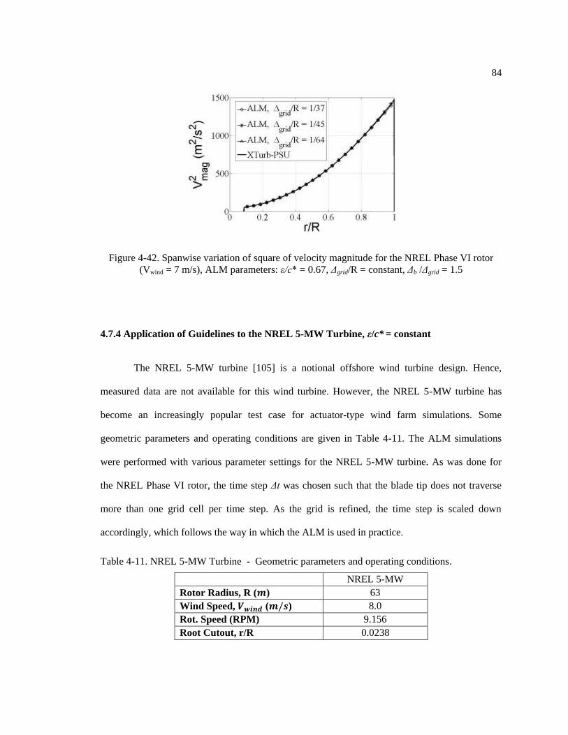
84

Figure 4-42. Spanwise variation of square of velocity magnitude for the NREL Phase VI rotor


4.7.4 Application of Guidelines to the NREL 5-MW Turbine, ε/c* = constant

The NREL 5-MW turbine [105] is a notional offshore wind turbine design. Hence,

measured data are not available for this wind turbine. However, the NREL 5-MW turbine has

become an increasingly popular test case for actuator-type wind farm simulations. Some

geometric parameters and operating conditions are given in Table 4-11. The ALM simulations

were performed with various parameter settings for the NREL 5-MW turbine. As was done for

the NREL Phase VI rotor, the time step Δt was chosen such that the blade tip does not traverse

more than one grid cell per time step. As the grid is refined, the time step is scaled down

accordingly, which follows the way in which the ALM is used in practice.

Table 4-11. NREL 5-MW Turbine - Geometric parameters and operating conditions.

NREL 5-MW

Rotor Radius, R ( ) 63

Wind Speed, ( ) 8.0

Rot. Speed (RPM) 9.156

Root Cutout, r/R 0.0238

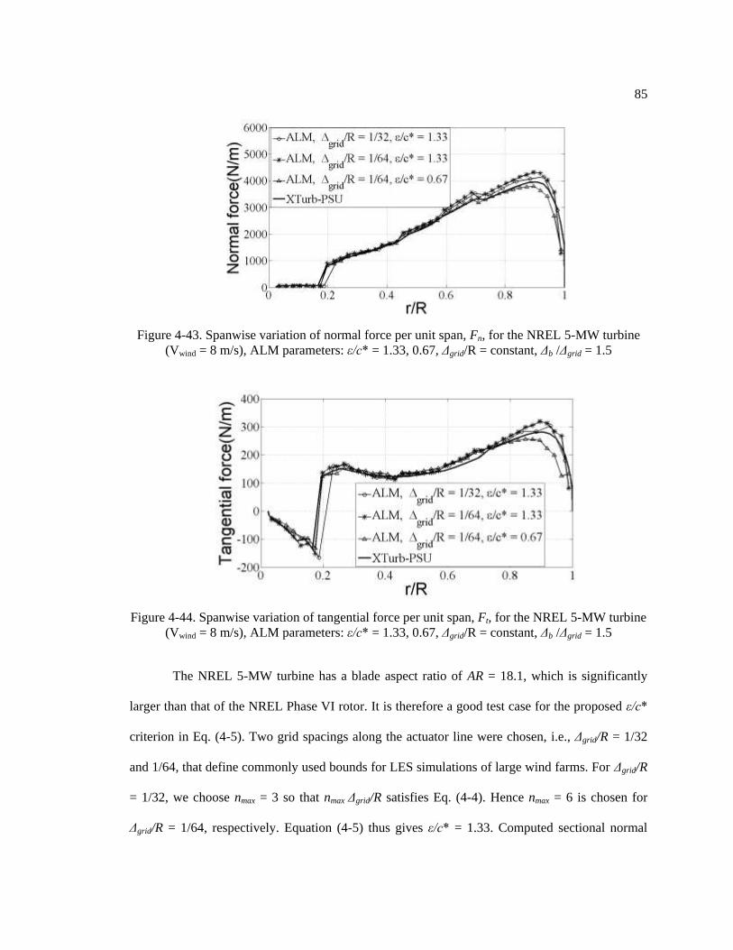
85

Figure 4-43. Spanwise variation of normal force per unit span, Fn, for the NREL 5-MW turbine

(Vwind = 8 m/s), ALM parameters: ε/c* = 1.33, 0.67, Δgrid/R = constant, Δb /Δgrid = 1.5

Figure 4-44. Spanwise variation of tangential force per unit span, Ft, for the NREL 5-MW turbine

(Vwind = 8 m/s), ALM parameters: ε/c* = 1.33, 0.67, Δgrid/R = constant, Δb /Δgrid = 1.5

The NREL 5-MW turbine has a blade aspect ratio of AR = 18.1, which is significantly

larger than that of the NREL Phase VI rotor. It is therefore a good test case for the proposed ε/c*

criterion in Eq. (4-5). Two grid spacings along the actuator line were chosen, i.e., Δgrid/R = 1/32

and 1/64, that define commonly used bounds for LES simulations of large wind farms. For Δgrid/R

= 1/32, we choose nmax = 3 so that nmax Δgrid/R satisfies Eq. (4-4). Hence nmax = 6 is chosen for

Δgrid/R = 1/64, respectively. Equation (4-5) thus gives ε/c* = 1.33. Computed sectional normal

86

and tangential forces are shown in Figures 4-43 and 4-44, respectively. The force convention

again follows NREL‘s definition [107] where the normal force acts orthogonal to the local chord

line and towards the sectional airfoil‘s upper surface, while the tangential force is parallel to the

local chord line and oriented towards the leading edge. It can be seen that the shape of the loading

profiles along the span are consistent and behave properly at the tips when using the ALM

parameters chosen according to the guidelines developed in section 4.6. However, it is apparent

that using ε/c* = 1.33 with both grid resolutions creates larger loads than predicted with XTurb-

PSU. For comparison, a case for ε/c* = 0.67 is also shown, and it can be seen that computed loads

are too low, especially near the sensitive tip region. This clearly demonstrates that the value of

ε/c* is a function of the blade aspect ratio, as suggested by Eq. (4-5). However, the fact that using

ε/c* = 1.33 or ε/c* = 0.67 overpredicts or underpredicts, respectively, blade loads across the entire

span compared to XTurb-PSU suggest that the guideline provided in Eq. (4-4) for choosing the

value of nmax is not a hard rule, but a mere guideline. It is only through future work, possibly with

application to other rotors, that a more precise means of computing nmax can be found.

As a final investigation, the best practices for a grid-based, chord-based, and elliptic

Gaussian radius ε are applied to the NREL 5-MW turbine using Δgrid/R = 1/64. The

Glauert/Prandtl correction was only used for the best-practice case of a grid-based Gaussian

radius ε. The results are presented in Figures 4-45 and 4-46. In comparison to the NREL Phase VI

rotor, a chord-based Gaussian radius ε/c = constant exhibits improved results. This is attributed to

the fact that the chord distribution near the blade tip of the NREL 5-MW turbine is not too

different from an elliptic shape (Fugure 4-25(b)). It is clear, though, that the proposed elliptic

Gaussian radius with ε/c* = constant gives consistent results between various blade designs and

grid spacing. It is therefore a more general method for determining ALM parameters. In

particular, it suggests a suitable value for ε/c* for a given grid resolution Δgrid/R and blade aspect

ratio AR.

87

Figure 4-45. Spanwise variation of normal force per unit span, Fn, for the NREL 5-MW turbine

(Vwind = 8 m/s), ALM parameters: Δgrid/R = 1/64

Figure 4-46. Spanwise variation of tangential force per unit span, Ft, for the NREL 5-MW turbine

(Vwind = 8 m/s), ALM parameters: Δgrid/R = 1/64

Table 4-12 summarizes computed rotor power and thrust for the best-practice cases in

Figures 4-45 and 4-46. The wake structure, characteristic of the momentum deficit, corresponding

to the results in Figures 4-45 and 4-46 are presented in Figure 4-47. The advantage of using the

proposed method of Gaussian spreading is evident. It can be seen that both tip and root vortices

appear tighter for the case of a variable Gaussian radius ε along the blade span. Furthermore, the

bound vorticity along the blade is less tube-like and appears to have more of an elliptic shape.

88

Table 4-12. Rotor power and thrust - NREL 5-MW turbine (Vwind = 8 m/s), ALM parameters: ε,

Δgrid /R = 1/64

NREL 5-MW turbine Power (kW) Thrust (kN)

XTurb-PSU 1,890 384

ALM (ε/Δgrid = 2, Prandtl

factor)

1,737 358

ALM (ε/c = 1.33) 2,066 403

ALM (ε/c* = 1.33) 2,113 409

(a) ε/Δgrid = 2

(b) ε/c = 1.33

(c) ε/c* = 1.33

Figure 4-47. Wake structure and strength for the NREL 5-MW turbine (Vwind = 8m/s) showing

iso-surface of vorticity magnitude 0.5 s-1

89

4.8 Chapter Summary

The objective of this chapter was to assess and improve the accuracy of the state-of-the-

art actuator-line method ALM in predicting rotor blade loads. The ALM was applied within an

OpenFOAM computational fluid dynamics (CFD) solver to various blade planform geometries

including the NREL Phase VI rotor in rotating and parked conditions, two wing designs with an

elliptic load distribution, and the NREL 5-MW turbine. Results obtained for sectional AOA as

well as normal and tangential force coefficients were compared to data, when available, and to

results obtained by the wind turbine design and analysis code XTurb-PSU.

It was found that the current ALM shows a consistent overprediction in rotor tip loads for

all blade planforms considered when using a constant spreading radius (or width) ε/Δgrid of the

Gaussian within the ALM discretization. Consequently, integrated rotor thrust and power are

overpredicted, which is likely to have an effect on the recovery process of the wake momentum

deficit in the rotor wake, which is a subject of a future chapter (chapter 6). Furthermore, it was

noted that increasing the constant ε/Δgrid further increases the integrated rotor loads. A new

method was developed for a variable spreading width ε along the blade span that is based on a

‗fictitious‘ elliptic planform c* with the same aspect ratio AR as the actual blade. The proposed

ε/c* criterion is a function of the blade AR, the grid resolution Δgrid, and free parameters nmax and

nmin that describe the maximum and minimum spreading width at the mid-blade and tip locations,

respectively, in multiples of the grid spacing Δgrid along the blade. It was demonstrated that the

proposed ε/c* criterion gives improved predictions of computed rotor loads for all blade designs

considered. In addition, choosing nmax = {3, 4} and nmin = 1 consistently gave the best predictions

for all cases. A stretched grid with refinement at the blade tips of about Δgrid /R further improved

the prediction of the local inflow in terms of AOA.

90

Chapter 5

Turbulence Statistics and Unsteadiness of Blade

Loads for Turbine-Turbine Interaction

The previous chapter presented an accuracy assessment of the state-of-the-art ALM,

development of a new method of force projection, and guidelines for using the proposed method.

This chapter presents the application of the state-of-the-art as well as modified ALM to a turbine-

turbine interaction problem. First, uniform inflow is considered for a general understanding of

turbine-turbine interaction using the state-of-the-art ALM. This is followed by a detailed study of

the problem with turbulent inflow and the use of two types of ALM approaches. The detailed

study includes analysis of blade loads, integrated quantities such as power, wake profiles, and

blade load unsteadiness.

5.1 Turbine-Turbine Interaction with Uniform Inflow

The turbine-turbine interaction problem consists of two NREL 5-MW turbines spaced 6D

apart with a uniform inflow of 8 m/s and the turbine RPM fixed at 9.16. The grid used was

similar to the one used for simulations of the NREL 5-MW turbines in section 4.7.4 with a

resolution of R/32 in the vicinity of the turbine and in the wake. The simulation was performed

for 500 sec of real time to ensure that the wake exits the domain. A time series of power for both

turbines is shown in Figure 5-1. Initially, both power histories converge to the expected power of

2MW. At about 100 sec, the wake of turbine 1 starts interacting with turbine 2. Consequently, the

91

power for turbine 2 converges into a limit cycle. It should be noted that the power for turbine 2 is

lower than would be expected in a real wind turbine array.

Figure 5-1. Time series of turbine power (Turbine-Turbine Interaction Problem, Uniform Inflow,

VWind = 8m/s). ALM parameters: ε/Δgrid = constant, Δgrid /R = 1/32, Δb /Δgrid = 1.

This lower power is attributed to the absence of recovery of the wake momentum deficit

before it reaches turbine 2. However, an interesting observation is that the power of turbine 2

enters an approximate limit cycle whose time period is approx. 25sec, i.e. ≈ 5 rotor revolutions. In

order to understand this limit cycle better, the flow field was investigated. Figure 5-2 shows the

contours of vorticity magnitude in an axial plane. It can be noticed that the flow field comprises

the structures of merged tip vortices that are spaced around 50 m and are convected at a speed of

2 m/s. The convection speed of 2 m/s (approx.) was determined by looking at the flow field at

two different time instants and tracking a vortex structure. This explains the power variation of

turbine 2. In order to further enhance the understanding of the flow field and turbulent structures,

an iso-surface of Q = 0.01 was observed. Here, Q is the second invariant of the strain-rate tensor.

92

This is shown in Figure 5-3. The breakdown of vortices downstream of both turbines and

increased turbulence level in the wake of turbine 2 are apparent.

Figure 5-2. Contours of vorticity magnitude in an axial plane (Turbine-Turbine Interaction

Problem, Uniform Inflow, VWind = 8m/s).

Figure 5-3. Iso-surface of Q = 0.01 1/s2 (Turbine-Turbine Interaction Problem, Uniform Inflow,

VWind = 8m/s).

93

5.2 Simulation Methodology with Turbulent Inflow

The simulation of wind turbine(s) with turbulent inflow using the LES-OpenFOAM

framework involves two steps. A precursor ABL simulation is first performed on a grid of normal

hexahedral cells that typically extends 3 km x 3 km x 1 km in the two horizontal directions and

the vertical direction, respectively, with a resolution of about 10 m. The simulation is run until a

quasi-stationary state is achieved, which commonly takes between 10,000 s and 30,000 s,

depending in large part upon the atmospheric stability state simulated. The simulation is then

continued for 2,000 s to extract precursor boundary-layer data at the inlet plane(s) at a sampling

frequency between 1-2 Hz. These boundary data serve as inflow to the actual ALM simulations.

Simulation statistics are collected and analyzed as the simulation progresses.

The ALM simulations, forced by precursor boundary-layer data, are performed on grids

of type and resolution that have been found to give accurate and consistent results, see chapter 4.

An illustration is given in Figure 5-4. Typically, 2 to 3 layers of grid refinement are performed in

the region surrounding the turbines and their wakes, starting with the original grid used for the

ABL precursor simulation. The refinement is done by splitting cells in half in each direction

within each successive refinement zone. A grid resolution of 2.5 m near the turbine is used as a

baseline. This is the finest grid resolution of the innermost grid, and it is maintained up to the end

of the region of interest to allow the proper resolution of smaller scale important turbulent

structures generated by the turbine blades and the turbine wakes. It should also be noted that the

extent of the innermost refinement zone along the spanwise direction is about 2.5D to capture the

meandering wake. Time-averaging of the AOA, blade loads, and power etc. for each turbine as

well as the velocity components, and Reynolds stress components at various locations in the wake

of both turbines starts after 300 seconds of real time when initial transients have subsided, and the

94

wake from the upstream turbine starts interacting with the downstream turbine. The time-

averaging has been performed for 1700 sec (about 260 revolutions).

Figure 5-4. Computational domain used for turbine-turbine interaction problem.

Two different techniques are used to determine the body force projection width, or

Gaussian radius ε, along the span of the blade. These were explained in chapter 4. The two

methods are:

1. Grid-based 𝛆

2. Elliptic 𝛆 ∗ [Ref. 108]

(5-1)

The first of these, the grid-based method, is the standard method that is widely used, and

the second method is a result of recent improvements [108] and was presented in chapter 4. The

focus of this chapter is to answer the questions of how these two techniques for determining the

body-force projection width, or Gaussian radius ε, affect the time-varying blade loads and

integrated power, the associated turbulence statistics in the wake, and the degree of unsteadiness

of blade loads.

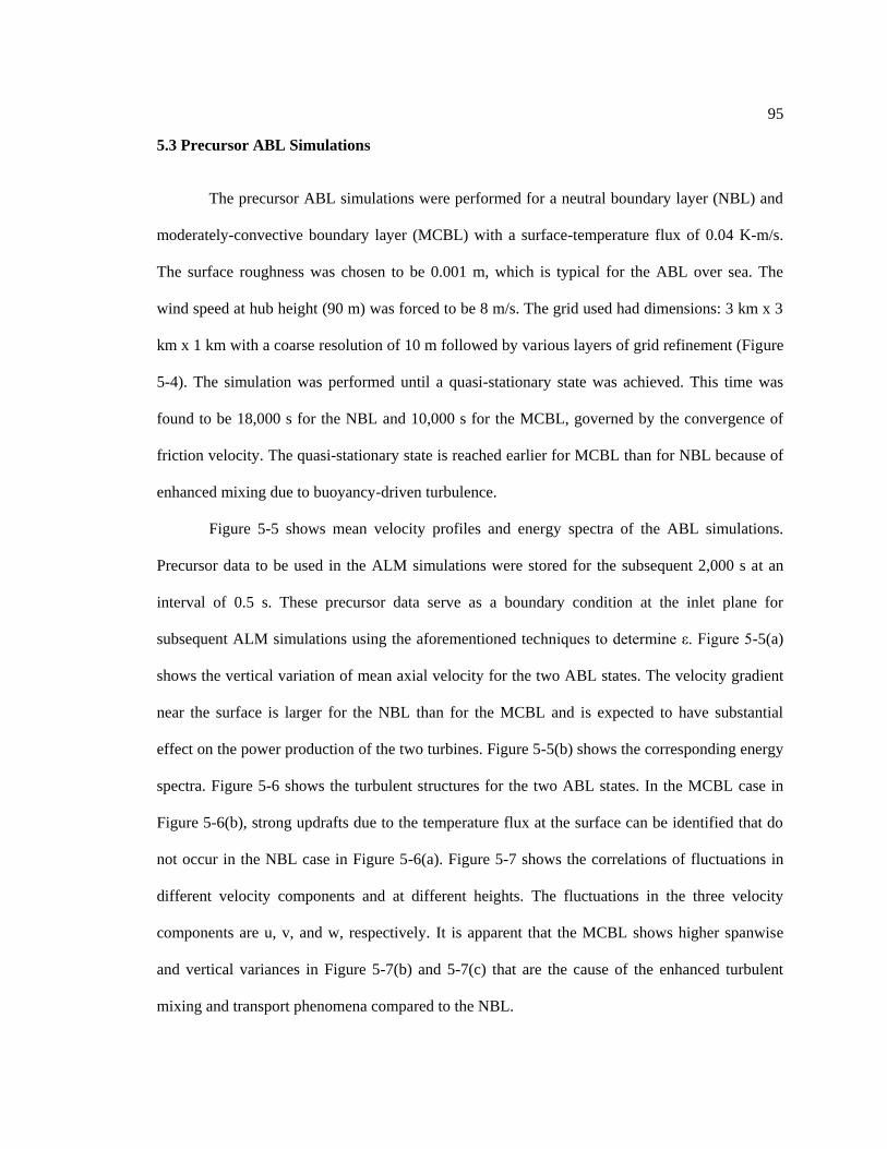
95

5.3 Precursor ABL Simulations

The precursor ABL simulations were performed for a neutral boundary layer (NBL) and

moderately-convective boundary layer (MCBL) with a surface-temperature flux of 0.04 K-m/s.

The surface roughness was chosen to be 0.001 m, which is typical for the ABL over sea. The

wind speed at hub height (90 m) was forced to be 8 m/s. The grid used had dimensions: 3 km x 3

km x 1 km with a coarse resolution of 10 m followed by various layers of grid refinement (Figure

5-4). The simulation was performed until a quasi-stationary state was achieved. This time was

found to be 18,000 s for the NBL and 10,000 s for the MCBL, governed by the convergence of

friction velocity. The quasi-stationary state is reached earlier for MCBL than for NBL because of

enhanced mixing due to buoyancy-driven turbulence.

Figure 5-5 shows mean velocity profiles and energy spectra of the ABL simulations.

Precursor data to be used in the ALM simulations were stored for the subsequent 2,000 s at an

interval of 0.5 s. These precursor data serve as a boundary condition at the inlet plane for

subsequent ALM simulations using the aforementioned techniques to determine ε. Figure 5-5(a)

shows the vertical variation of mean axial velocity for the two ABL states. The velocity gradient

near the surface is larger for the NBL than for the MCBL and is expected to have substantial

effect on the power production of the two turbines. Figure 5-5(b) shows the corresponding energy

spectra. Figure 5-6 shows the turbulent structures for the two ABL states. In the MCBL case in

Figure 5-6(b), strong updrafts due to the temperature flux at the surface can be identified that do

not occur in the NBL case in Figure 5-6(a). Figure 5-7 shows the correlations of fluctuations in

different velocity components and at different heights. The fluctuations in the three velocity

components are u, v, and w, respectively. It is apparent that the MCBL shows higher spanwise

and vertical variances in Figure 5-7(b) and 5-7(c) that are the cause of the enhanced turbulent

mixing and transport phenomena compared to the NBL.

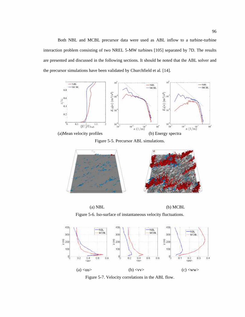
96

Both NBL and MCBL precursor data were used as ABL inflow to a turbine-turbine

interaction problem consisting of two NREL 5-MW turbines [105] separated by 7D. The results

are presented and discussed in the following sections. It should be noted that the ABL solver and

the precursor simulations have been validated by Churchfield et al. [14].

(a)Mean velocity profiles (b) Energy spectra

Figure 5-5. Precursor ABL simulations.

(a) NBL (b) MCBL

Figure 5-6. Iso-surface of instantaneous velocity fluctuations.

(a) <uu> (b) <vv> (c) <ww>

Figure 5-7. Velocity correlations in the ABL flow.

97

5.4 Simulations of Two NREL-5 MW Turbines with Turbulent Inflow

The simulations with two turbines were performed for 2,000 s for which stored precursor

ABL inflow data were available. The averaging was started at 300 sec when the initial transients

disappeared. The near-blade grid resolution was 2.5 m, and the time step of the ALM simulation

was smaller compared to the precursor ABL simulations such that the actuator-line tips did not

traverse more than one grid cell per time step. This constraint is similar to a CFL criterion based

on the rotor tip speed. The time-step size was chosen to be 0.02 s corresponding to an average

azimuthal step of 1.1 degree. Stored precursor ABL inflow data were used as inflow boundary

conditions; the opposite boundaries were outflow boundaries. As the precursor boundary-data

time interval need not coincide with the ALM simulation time step, the boundary data are linearly

interpolated in time.

The selected time interval of 1,700 seconds, corresponding to 260 revolutions, is

adequate to yield meaningful turbulence statistics, since the wake is fully evolved. The

horizontally-averaged mean velocity at hub height from the ABL simulation was 8 m/s, for NBL

as well as MCBL. This was achieved by altering the pressure gradient in the ABL solver, and this

velocity at hub height served as a reference velocity. The actual ALM simulation did not have

this constraint. The velocity profiles were sampled along a vertical line passing through a line

connecting the turbine hubs, for the entire 2,000 s of simulation time, saving line data every 1 sec

(or 50 time steps).

Before delving into the blade loads and statistics etc., some idea can be gained about

them by looking at the flow field. Figure 5-8 illustrates iso-surface of vorticity magnitude 0.5 1/s

extracted from the computed flow field in NBL using the modified ALM. The second turbine

(Turbine 2) is located 7D downstream of the first turbine (Turbine 1). A CAD model of the

NREL 5-MW turbine has been added to the figure to illustrate the position of the actuator lines

98

(or rotor blades) at this particular instant in time. It can be seen in Figure 5-8 that the tip vortices

trailing downstream of the first turbine remain stable for approximately four revolutions. It is also

apparent that the flow becomes dominated by turbulent eddy motion before interacting with the

second (downstream) turbine and even more so downstream of the second turbine. Figure 5-8

also indicates that tip vortices break down sooner downstream of Turbine 2 than they do

downstream of Turbine 1. It is shown later that the enhanced turbulence in the inflow plane to

Turbine 2 results in a higher standard deviation of turbine power.

Figure 5-8. Turbine-Turbine interaction in a neutral ABL (NREL 5-MW Turbines, VWind = 8m/s).

Figure 5-9 shows an axial plane through the rotor hub colored with instantaneous

contours of velocity magnitude, again for NBL and using the modified ALM. It can be seen that

the upper (above hub height) sheet of tip vortices becomes unstable and eventually breaks down

in large structures that further break down in the wake into progressively finer structures of

turbulence. It is interesting to note that the lower (below hub height) sheet of tip vortices becomes

unstable much sooner than its upper counterpart. This is attributed to higher shear in the lower

parts of the atmospheric surface layer. This is expected to affect the wake profile for the upper

and lower halves and hence the wake recovery pattern. In addition, Figure 5-9 shows that the root

vortices appear less strong, which is attributed to the transition region from the root airfoil section

99

into a cylindrical section close to the hub that essentially does not produce any aerodynamic lift.

The actual root vortices are hence spread over that transition region and thus appear to be weaker

than the tip vortices.

Figure 5-9. Instantaneous contours of velocity magnitude. (NBL, NREL 5-MW Turbine 1, VWind =

8m/s)

(a) ε/Δgrid = const. (b) ε/c*= const.

Figure 5-10. Instantaneous flow field in a horizontal plane at hub height (t = 2,000 sec, NBL

inflow). The quantity shown is the component of vorticity normal to the plane.

Figure 5-10 shows instantaneous flow fields at t = 2,000 sec. The two turbines are not

synchronized; rather, the downstream turbine attempts to achieve the design tip speed ratio. Iso-

100

contours of the z-component of vorticity are shown for the two types of body-force projection

methods discussed earlier and for NBL inflow. It can be seen that the wakes for the two cases

exhibit indiscernible differences. However, it is unclear from Figure 5-10 what the quantitative

differences of the two ALM approaches are. In the subsequent sections, sectional AOA, which is

the most fundamental physical parameter relevant to the ALM, and blade loads, will be discussed.

In particular, the statistics, probability density function (PDF), and power spectral density (PSD)

are quantified. Next, the integrated quantities are analyzed. The blade loads affect the tip vortices

and vortex sheets emanating from the turbines (as shown in Figures 5-8 and 5-9). Therefore, the

effect of the ALM projection method on wake turbulence, and hence the inflow to the

downstream turbine, are assessed.

5.4.1 Sectional Blade Loads

The underlying method of any ALM starts with the determination of the flow-field

velocity vector at the actuator points, see the schematic of ALM in Figure 3-3. These velocity

components determine the local AOA at a given actuator point at each time step. Figure 5-11

shows spanwise distributions of sectional mean and standard deviation (indicated as error bars) of

AOA along the blades of both turbines, for both ABL stability states, and for both ALM

projection methods. Results are shown for one blade at a time, contrasting the two ALM

spreading methods considered in this work. It can be observed in all the cases that a constant

Gaussian spreading radius ε/Δgrid leads to higher AOA at the blade tips compared to those

computed with the elliptic Gaussian radius ε/c*. It should be noted that no tip correction was

applied to the airfoil data. At this stage, no dynamic-stall or stall-delay model was used to modify

the airfoil tables, a restriction that will be discussed later. Both types of ALM spreading methods

yield similar AOA distributions inboard of r/R = 0.85. In general, the inboard stations show

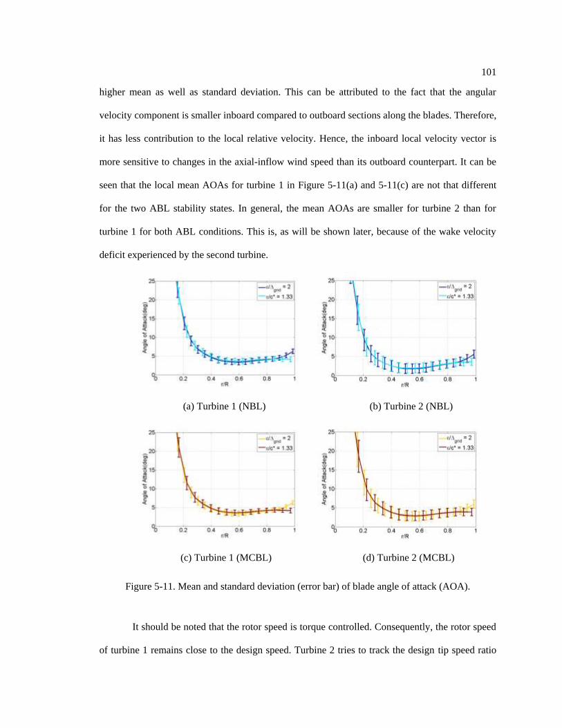
101

higher mean as well as standard deviation. This can be attributed to the fact that the angular

velocity component is smaller inboard compared to outboard sections along the blades. Therefore,

it has less contribution to the local relative velocity. Hence, the inboard local velocity vector is

more sensitive to changes in the axial-inflow wind speed than its outboard counterpart. It can be

seen that the local mean AOAs for turbine 1 in Figure 5-11(a) and 5-11(c) are not that different

for the two ABL stability states. In general, the mean AOAs are smaller for turbine 2 than for

turbine 1 for both ABL conditions. This is, as will be shown later, because of the wake velocity

deficit experienced by the second turbine.

(a) Turbine 1 (NBL) (b) Turbine 2 (NBL)

(c) Turbine 1 (MCBL) (d) Turbine 2 (MCBL)

Figure 5-11. Mean and standard deviation (error bar) of blade angle of attack (AOA).

It should be noted that the rotor speed is torque controlled. Consequently, the rotor speed

of turbine 1 remains close to the design speed. Turbine 2 tries to track the design tip speed ratio

102

(TSR) in response to the velocity deficit in the wake but because of rotor inertia it cannot do this

instantaneously. The difference in AOA for turbine 2 in Figure 5-11(b) and 5-11(d) is more

pronounced for NBL than for MCBL flow because vertical turbulent mixing in the MCBL

accelerates the recovery process of the wake velocity deficit. We can therefore conclude that the

mean wind (or axial) component of the resultant velocity compared to the local angular velocity

component is higher in the MCBL than in the NBL, thus resulting in turbine 2 having a higher

mean AOA in MCBL flow than in NBL flow. The standard deviations in AOAs are, in general,

larger for turbine 2 than for turbine 1 and for both ABL states because turbine 2 encounters

turbulence due to both the ABL as well as the wake of turbine 1. Also, the turbine wakes

meander, so the blades of turbine 2 vary between being waked and unwaked conditions.

The statistics presented above take into account the entire simulation time interval after

the wake of the upstream turbine 1 starts interacting with the downstream turbine 2, i.e. t = 300

sec – 2,000 sec. One question that arises, though, is how likely the local AOA is to lie within a

certain range as this has implications on attached and separated flow regions along the blade span.

This can only be studied by looking at the probability density function (PDF) of the local AOA at

selected radial stations of relevance. Figure 5-12 shows the PDFs of the AOA for the two turbines

and at the spanwise locations r/R = 0.340 and r/R = 0.914 that represent one inboard and one

outboard blade station. Comparisons are performed for the two types of ALM spreading for the

Gaussian radius ε and the two ABL states. For both turbines and both ABL stability states,

constant ε/Δgrid spreading moves the PDF curve to a higher mean AOA at the outboard location

r/R=0.914, which reflects the higher AOA observed in Figure 5-11. The ALM spreading method

does not shift the curves at the inboard location r/R = 0.340. Smaller AOAs for turbine 2 are

again observed, consistent with Figure 5-11. Both inboard and outboard, the ABL state does not

cause a shift in the curve for turbine 1. However, this is different for turbine 2 where the PDFs are

shifted to higher mean AOA for MCBL inflow, i.e. the AOAs for turbine 2 are higher in an

103

MCBL than in an NBL at both inboard and outboard locations. This is again consistent with the

observations in Figure 5-11. Moreover, the PDF curves for turbine 2 are, in general, flatter than

the corresponding curves for turbine 1, reflecting higher standard deviation. Also, the PDF curves

for turbine 2 are not as smooth, which is attributed to the enhanced turbulence experienced by the

second turbine.

(a) Turbine 1, r/R = 0.34 (b) Turbine 1, r/R = 0.91

(c) Turbine 2, r/R = 0.34 (d) Turbine 2, r/R = 0.91

Figure 5-12. Probability density function (PDF) of blade angle of attack (AOA).

So far, the statistics and PDF of local AOA at selected blade stations have been

discussed. They give an overall idea of how the blade loads and the integrated power are expected

to reflect this behavior. However, one needs to look at the PSD of AOA to gain an insight into the

frequency content in the time histories of the sectional AOAs. Figure 5-13 shows the PSD of

computed AOAs for turbine 1 and spanwise locations r/R = 0.340 and r/R = 0.914 for both NBL

104

and MCBL inflow. The sampling frequency was 50 Hz corresponding to the simulation time step

of 0.02 s, thus resulting in 85,000 samples. In order to get smooth spectra, 85 windows of 1,000

samples each were used, and the mean of the PSD of each of these windows was computed.

(a) Turbine 1, r/R = 0.34 (NBL) (b) Turbine 1, r/R = 0.91 (NBL)

(c) Turbine 1, r/R = 0.34 (MCBL) (d) Turbine 1, r/R = 0.91 (MCBL)


spanwise stations.

Comparisons are again performed for the two types of ALM spreading methods. Figure

5-14 shows the corresponding plots for turbine 2. For both turbines, both NBL and MCBL inflow

conditions, and for each of the spreading methods, the dominant frequency inboard is the

rotational frequency 1/rev, i.e. about 0.15 Hz (or 9 RPM). The higher harmonics of n*(1/rev)

apart from the dominant frequency are also visible in Figures 5-13 and 5-14 at the outboard

105

station r/R = 0.91, while they are much less pronounced at the inboard station r/R = 0.34. This is

attributed to the fact that the blade tip has a more sensitive response to smaller-scale ABL

turbulence, which is in part due to the combination of a smaller blade chord outboard and higher

velocities, both leading to a smaller time scale associated with the blade tip region. It can also be

observed that the higher harmonics of turbine 2 are not perfectly aligned with the higher

harmonics of rotational frequency. This is attributed to the variable rotor speed of turbine 2 in

response to the turbulent wake from turbine 1. The frequency response and hence the PSD of

integrated power is expected to comprise the various frequency responses at inboard as well as

outboard locations. This will be further analyzed in the section on integrated quantities. For both

turbines in Figures 5-13 and 5-14, inboard as well as outboard, the NBL and MCBL stability

states do not seem to result in a noticeable difference in the PSD; however, the spreading method

affects the spectra predominantly at the outboard station r/R = 0.91 (Figures 5-13(c), 5-13(d), 5-

14(c) and 5-14(d)). The PSD for the two spectra differ for frequencies higher than about 6 Hz.

This means that the ALM method using ε/c* is more sensitive to the higher frequencies (or

smaller-scale turbulence) than the one using a constant Gaussian radius defined by ε/Δgrid. It is

interesting to note that the ALM spreading methods do not affect the PSD at the inboard station

r/R = 0.340. This observation is in agreement with those made for the AOA variation along the

blade span where tip loads (r/R > 0.85) are quite different between the two ALM methods.

Therefore, a further investigation into the frequencies above 6 Hz is necessary to understand the

turbulence scales and unsteady aerodynamics resolved by the two ALM approaches. A

convective time scale is defined as the time taken to traverse half the local chord length by the

local relative velocity, i.e.

(5-2)

The corresponding convective frequency is defined as:

106

(5-3)

(a) Turbine 2, r/R = 0.34 (NBL) (b) Turbine 2, r/R = 0.91 (NBL)

(c) Turbine 2, r/R = 0.34 (MCBL) (d) Turbine 2, r/R = 0.91 (MCBL)


spanwise stations.

Figures 5-13 and 5-14 show vertical lines at frequencies corresponding to different

multiples of local . It is obvious that the ALM method using ε/c* can sense frequencies

corresponding to the time scales in the range of higher multiples of , at the outboard location.

The peaks in the aforesaid range do not match the exact multiples of . This can be attributed to

the fact that the actual chord geometry is not meshed. It can only be established through a highly

blade-resolved simulation whether these frequencies are manifestations of the accuracy of the

ALM approaches used. It should be noted that the highest frequency sensed corresponding to the

107

sampling frequency of 50 Hz might have missed further small-scale motions. A study with higher

sampling frequency will potentially unravel this. However, this would require a smaller time step,

putting a more stringent requirement on the blade tip than traversing at the most one grid cell per

time step. Apart from the peaks of the frequencies discussed, it can be observed that the inertial

sub-range of the spectra gets prolonged for the ALM method using ε/c*, meaning sensing smaller

turbulence scales. The above observation holds true for both the turbines and both the ABL states.



Figure 5-15. Mean and standard deviation (error bar) of local lift coefficient (cl).

Once the AOAs are determined locally at the actuator points, the next step in the ALM is

to look up the aerodynamic force coefficients from the airfoil data tables and to compute local

blade forces. Figure 5-15 shows the mean and standard deviation as error bars in local sectional

lift coefficient for one selected blade of the two turbines and for the two ABL states, i.e. NBL and

MCBL. Again, comparisons are made for the two types of spreading methods. The observations

108

here are in line with those for the local AOAs in Figure 5-11, as expected. It is apparent that

turbine 1 operates at overall higher AOAs compared to turbine 2. However, the standard

deviation in the sectional lift coefficient is significantly higher along the blade span of turbine 2

than it is for turbine 1. Furthermore, it can be seen that the most inboard stations operate at high

lift coefficients. It is therefore reasonable to assume that inboard blade stations operate under

unsteady aerodynamic conditions including separation and dynamic stall, both of which are not

accounted for in the simulations.

5.4.2 Integrated Quantities

The sectional blade loads, for the most part proportional to the sectional AOA, are

integrated along the span yielding power, thrust, and root-flap bending moment. Here, the time

histories, statistics, and PSD of integrated power and bending moment are discussed. The time

history of thrust is presented for the sake of completeness. The frequency response of the

integrated power and bending moment and their relation to the frequency response of sectional

AOA are also addressed. Figure 5-16 shows the power histories of the two turbines for the two

ABL states. In each subfigure, comparisons are made between the two ALM spreading methods.

For both turbines, the power for the second turbine is lower than the first turbine due to a velocity

deficit in the wake that has not fully recovered at turbine 2. However, this power drop for the

downstream turbine (turbine 2) is more pronounced for the NBL than for the MCBL. This is

attributed to the fact that, for the MCBL, higher turbulent mixing relative to the NBL helps to

recover the wake velocity deficit at a higher rate. Higher fluctuations in the power for both

turbines are visible for MCBL flow, which is again associated with higher turbulence levels due

to enhanced mixing as a result of surface heating. The effect of the ALM spreading method can

also be observed. For each turbine and for each ABL state, constant Gaussian spreading

109

according to the ε/Δgrid criterion leads to slightly higher peaks, which is attributed to the over-

prediction of blade tip loads as seen in Figure 5-11. The time trace of integrated power clearly

shows a range of frequencies. The lower frequencies are attributed to the average large-eddy

turnover time in the respective ABL flows, which are of higher amplitude in the MCBL flow

compared to the NBL flow and attributed to higher vertical velocity fluctuations in the MCBL

compared to the NBL.



Figure 5-16. Power histories for turbine-turbine interaction problem.

Similar to AOA, more insight about the frequencies can be gained from the spectra of

integrated power. Figure 5-17 shows the PSD of the two turbines for the two ABL states and with

comparisons between the two ALM spreading methods. Since the integrated power incorporates

the accumulated effects of all three blades, the dominant frequency here is 3/rev. It is apparent

110

from Figure 5-17 that the turbine rotation is responsible for the dominant PSD peak reflected at

3/rev (or 0.45 Hz). The higher harmonics of n*(3/rev) can also be seen and occur because of the

fluctuating velocity components that result in a different incoming mean shear flow for every

single blade revolution. These higher harmonics have most contributions from the outboard

spanwise blade locations as observed in the spectra of AOAs in Figures 5-13 and 5-14. Similar to

the spectra of AOA, the peak frequencies for turbine 2 are not perfectly aligned with the

harmonics of 3/rev. The effect of the elliptic ALM spreading method according to a ε/c* criterion

can be observed for the higher frequencies where the reduced tip loads compared to ALM

spreading according to ε/Δgrid in Figure 5-11 are more sensitive to the turbulent eddies. The

frequencies beyond 6-7 Hz resolved by the ALM method using ε/c* are a combined effect of the

sectional convective time scales.



Figure 5-17. Power spectral density (PSD) of turbine power.

111

(a) Mean turbine power (b) Std. dev. in turbine power

(c) Std. dev. relative to mean power

Figure 5-18. Mean and standard deviation of turbine power.

Figure 5-18 shows the mean, standard deviation, and the ratio of the two for the

integrated power, where the statistics comprise data from 300 s to 2,000 s of simulation time.

Comparisons are made for the two ABL states, i.e. NBL and MCBL, and the two spreading

methods. The observations for the mean and standard deviations for the two turbines are in

accordance with their respective time traces, i.e. the mean power for turbine 2 is smaller than that

of turbine 1. This is more pronounced in NBL flow as the wake does not recover as quickly in the

absence of enhanced vertical mixing due to surface heating. For turbine 1, the ABL stability state

does not have as much effect as on turbine 2. The standard deviation in power for both the

turbines is higher in MCBL flow compared to NBL flow. The absolute values of standard

deviation for turbine 2 compared to turbine 1 may be misleading. It is therefore more instructive

to look at standard deviation normalized by the corresponding mean power. For both ABL states,

112

the ratio of standard deviation to mean power is almost twice as much for turbine 2 compared to

turbine 1. With regards to the effect of the ALM spreading method, both the mean power and the

standard deviation are affected for both turbines and both ABL states. In general, the elliptic

spreading according to ε/c* leads to lower predicted values due to reduced tip loads. The

numerical values are given in Tables 5-1 and 5-2, respectively. The difference in mean power due

to the ALM spreading method is about 2.6 – 2.7 % for turbine 1 and about 3.90 - 4.26 % for

turbine 2. A difference of about 4% is not insignificant for an array of wind turbines since it may

result in an over-estimation of array efficiency. It is not surprising that turbine 2 exhibits an

accumulated effect of differences in the ALM spreading methods as discrepancies in wake

parameters downstream of turbine 1 are amplified through an additional ALM step at turbine 2. It

is hypothesized that the difference due to spreading would be further augmented if more turbines

are placed downstream because of the accruing difference as mentioned above. Further

simulations with more turbines may shed some light on this behavior but is beyond the scope of

the current work.

Table 5-1. Mean power for the turbines.

Mean Power (MW) Turbine 1 Turbine 2

NBL

Constant ε 1.9820 0.8731

Elliptic ε 1.9305 0.8359

% Difference 2.60 4.26

MCBL

Constant ε 2.1294 1.3554

Elliptic ε 2.0719 1.3025


Table 5-2. Standard deviation in power for the turbines.

Std. Dev. in Power (MW) Turbine 1 Turbine 2

NBL

Constant ε 0.1926 0.1273

Elliptic ε 0.1878 0.1196


MCBL

Constant ε 0.2883 0.2853

Elliptic ε 0.2821 0.2669


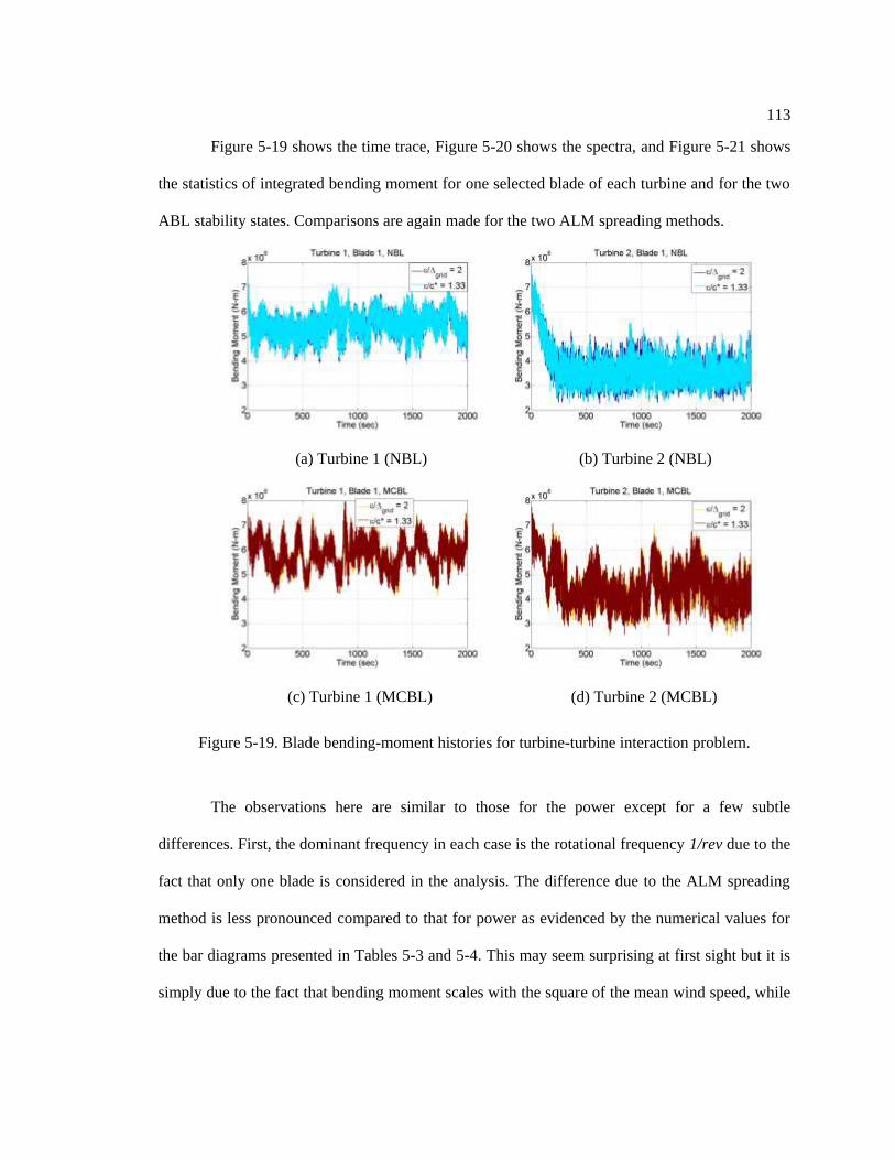
113

Figure 5-19 shows the time trace, Figure 5-20 shows the spectra, and Figure 5-21 shows

the statistics of integrated bending moment for one selected blade of each turbine and for the two

ABL stability states. Comparisons are again made for the two ALM spreading methods.



Figure 5-19. Blade bending-moment histories for turbine-turbine interaction problem.

The observations here are similar to those for the power except for a few subtle

differences. First, the dominant frequency in each case is the rotational frequency 1/rev due to the

fact that only one blade is considered in the analysis. The difference due to the ALM spreading

method is less pronounced compared to that for power as evidenced by the numerical values for

the bar diagrams presented in Tables 5-3 and 5-4. This may seem surprising at first sight but it is

simply due to the fact that bending moment scales with the square of the mean wind speed, while

114

power scales with the cube of the mean wind speed. Therefore, the observed discrepancies

between both ALM spreading methods are most pronounced for the turbine power.



Figure 5-20. Power spectral density (PSD) of blade bending moment.

As was observed for integrated power, the effect of the elliptic ALM spreading method

according to a ε/c* criterion can be observed for the higher frequencies where the reduced tip

loads compared to ALM spreading according to ε/Δgrid are more sensitive to the turbulent eddies.

Here again, the frequencies beyond 6-7 Hz resolved by the ALM method using ε/c* are a

combined effect of the sectional convective time scales.

115

(a) Mean turbine power (b) Std. dev. in turbine power

(c) Std. dev. relative to mean power

Figure 5-21. Mean and standard deviation of bending moment.

Table 5-3. Mean bending moment for one turbine blade.

Mean BM (x106 Nm) Turbine 1 Turbine 2

NBL

Constant ε 5.5441 3.5621

Elliptic ε 5.5285 3.5497


MCBL

Constant ε 5.8324 4.5134

Elliptic ε 5.8076 4.4754


Table 5-4. Standard deviation in root-flap bending moment for one turbine blade.

Std. Dev. in BM (x106 Nm) Turbine 1 Turbine 2

NBL

Constant ε 0.4746 0.5190

Elliptic ε 0.4750 0.5124

% Difference -0.08 1.27

MCBL

Constant ε 0.5637 0.7365

Elliptic ε 0.5586 0.7355


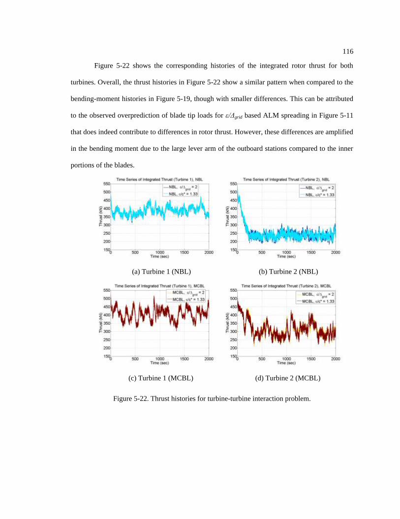
116

Figure 5-22 shows the corresponding histories of the integrated rotor thrust for both

turbines. Overall, the thrust histories in Figure 5-22 show a similar pattern when compared to the

bending-moment histories in Figure 5-19, though with smaller differences. This can be attributed

to the observed overprediction of blade tip loads for ε/Δgrid based ALM spreading in Figure 5-11

that does indeed contribute to differences in rotor thrust. However, these differences are amplified

in the bending moment due to the large lever arm of the outboard stations compared to the inner

portions of the blades.



Figure 5-22. Thrust histories for turbine-turbine interaction problem.

117

5.4.3 Wake Parameters

So far, we have looked exclusively at the loads and integrated quantities for the two

turbines. We have discussed the differences in the sectional loads, integrated quantities, and the

relation between them. It is equally important, however, to gain a deeper understanding of how

the turbine wakes develop under different ABL stability states and what impact the ALM

spreading methods have on the wake and how the differences between them affect the

performance of the downstream turbine.

(a) 2D downstream of Turbine 1 (b) 6D downstream of Turbine 1

(c) 2D downstream of Turbine 2 (d) 6D downstream of Turbine 2

Figure 5-23. Mean streamwise velocity distributions in the vertical direction.

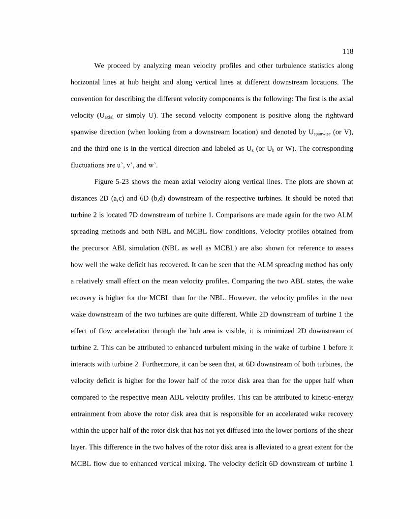
118

We proceed by analyzing mean velocity profiles and other turbulence statistics along

horizontal lines at hub height and along vertical lines at different downstream locations. The

convention for describing the different velocity components is the following: The first is the axial

velocity (Uaxial or simply U). The second velocity component is positive along the rightward

spanwise direction (when looking from a downstream location) and denoted by Uspanwise (or V),

and the third one is in the vertical direction and labeled as Uz (or Uh or W). The corresponding

fluctuations are u‘, v‘, and w‘.

Figure 5-23 shows the mean axial velocity along vertical lines. The plots are shown at

distances 2D (a,c) and 6D (b,d) downstream of the respective turbines. It should be noted that

turbine 2 is located 7D downstream of turbine 1. Comparisons are made again for the two ALM

spreading methods and both NBL and MCBL flow conditions. Velocity profiles obtained from

the precursor ABL simulation (NBL as well as MCBL) are also shown for reference to assess

how well the wake deficit has recovered. It can be seen that the ALM spreading method has only

a relatively small effect on the mean velocity profiles. Comparing the two ABL states, the wake

recovery is higher for the MCBL than for the NBL. However, the velocity profiles in the near

wake downstream of the two turbines are quite different. While 2D downstream of turbine 1 the

effect of flow acceleration through the hub area is visible, it is minimized 2D downstream of

turbine 2. This can be attributed to enhanced turbulent mixing in the wake of turbine 1 before it

interacts with turbine 2. Furthermore, it can be seen that, at 6D downstream of both turbines, the

velocity deficit is higher for the lower half of the rotor disk area than for the upper half when

compared to the respective mean ABL velocity profiles. This can be attributed to kinetic-energy

entrainment from above the rotor disk area that is responsible for an accelerated wake recovery

within the upper half of the rotor disk that has not yet diffused into the lower portions of the shear

layer. This difference in the two halves of the rotor disk area is alleviated to a great extent for the

MCBL flow due to enhanced vertical mixing. The velocity deficit 6D downstream of turbine 1

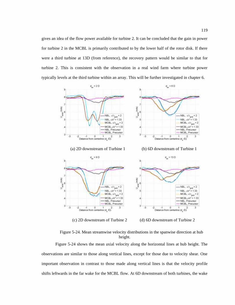
119

gives an idea of the flow power available for turbine 2. It can be concluded that the gain in power

for turbine 2 in the MCBL is primarily contributed to by the lower half of the rotor disk. If there

were a third turbine at 13D (from reference), the recovery pattern would be similar to that for

turbine 2. This is consistent with the observation in a real wind farm where turbine power

typically levels at the third turbine within an array. This will be further investigated in chapter 6.



Figure 5-24. Mean streamwise velocity distributions in the spanwise direction at hub

height.

Figure 5-24 shows the mean axial velocity along the horizontal lines at hub height. The

observations are similar to those along vertical lines, except for those due to velocity shear. One

important observation in contrast to those made along vertical lines is that the velocity profile

shifts leftwards in the far wake for the MCBL flow. At 6D downstream of both turbines, the wake

120

has meandered about 1D, i.e., the peak velocity deficit has drifted one rotor diameter from the

hub axis. Since the velocity profile at 6D downstream of each turbine is representative of the

power available for the next downstream turbine, the downstream turbine is expected to

encounter higher unsteady loadings due to the observed wake meandering. Therefore, while

MCBL helps in recovering the velocity deficit and hence enhancing the power production by the

downstream turbines, the unsteady loading due to up- and downdrafts in addition to wake

meandering may be detrimental to the structural health of downstream turbines. It is also apparent

that the eddy-structure and advection, determined by the ABL stability state, lead to wake-

meandering.



Figure 5-25. TKE distribution in the vertical direction.

121

We have thus far observed that the mean velocity profiles are affected by the ABL states

and exhibit different behavior at different downstream locations. While the ALM spreading

method had some noticeable effect on mean turbine power and its standard deviation, it has a

smaller effect on the mean velocity profiles in the wakes of the turbines. However, it is expected

that the difference in tip loads observed in Figure 5-11 result in subtle differences in the tip

vortices for the two ALM spreading methods. The tip vortices, though, do affect the wake. It is

therefore important to investigate the turbulent kinetic energy (TKE) and Reynolds stresses.



Figure 5-26. TKE distribution in the spanwise direction at hub height.

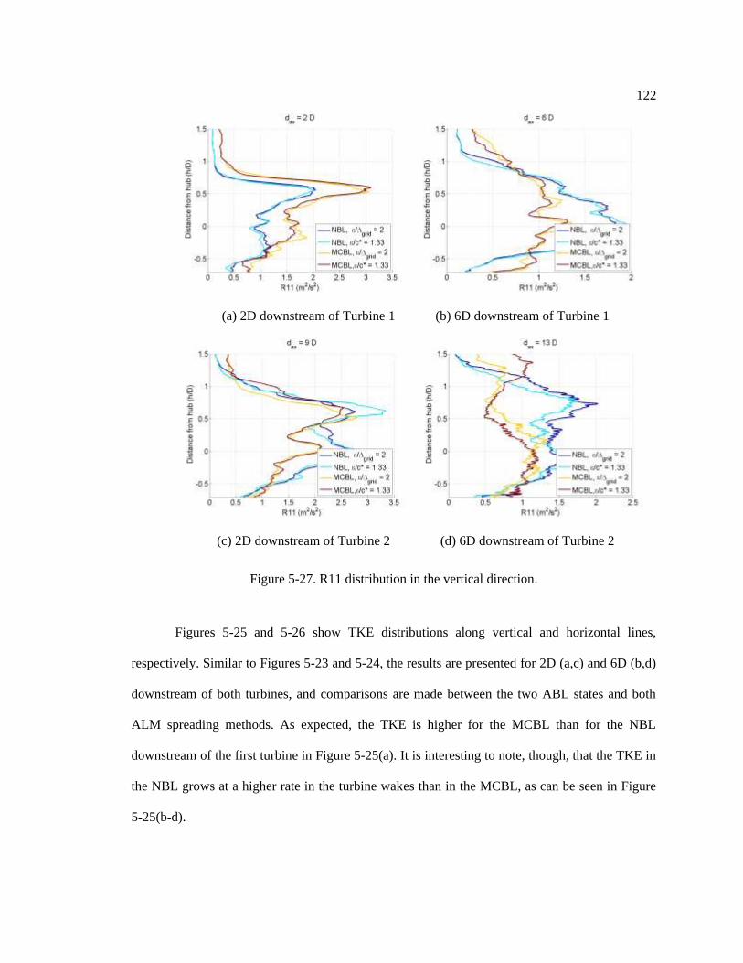
122



Figure 5-27. R11 distribution in the vertical direction.

Figures 5-25 and 5-26 show TKE distributions along vertical and horizontal lines,

respectively. Similar to Figures 5-23 and 5-24, the results are presented for 2D (a,c) and 6D (b,d)

downstream of both turbines, and comparisons are made between the two ABL states and both

ALM spreading methods. As expected, the TKE is higher for the MCBL than for the NBL

downstream of the first turbine in Figure 5-25(a). It is interesting to note, though, that the TKE in

the NBL grows at a higher rate in the turbine wakes than in the MCBL, as can be seen in Figure

5-25(b-d).

123



Figure 5-28. R11 distribution in the spanwise direction at hub height.

The meandering of the wake is also evidenced by the shift of TKE concentration along

the horizontal lines in Figure 5-26. One additional interesting observation is that the TKE for the

two ALM spreading methods differs mostly along the inner part of the rotor disk between z/D =

+/- 0.5. While the ALM spreading method according to ε/Δgrid shows slightly higher TKE

inboard, a Gaussian spreading following the ε/c* criterion exhibits slightly higher TKE injected

by the tip vortices, see Figure 5-25(a, c). It is hypothesized that this is related to the fact that

Gaussian spreading following ε/c* leads to tighter tip vortices than for the ε/Δgrid method due to a

smaller Gaussian radius ε at the blade tips. The situation is reversed around the mid-blade

124

location z/D = +/- 0.25, and, indeed, the TKE levels are higher for the ε/Δgrid method than for the

ε/c* criterion. This indicates that body-force projection as used in today‘s ALMs generates local

TKE somewhat inversely proportional to the Gaussian spreading radius ε. It also supports another

hypothesis, i.e. that coarse grids may generate tip vortices with too large cores and consequent too

low TKE. To date, there are, unfortunately, no data available that could be used for validation of

various ALM methods and the TKE that is being generated by the actuator lines.



Figure 5-29. R12 distribution in the spanwise direction at hub height.

Figures 5-27 and 5-28 show R11 on vertical and horizontal lines, respectively. The

Reynolds stress R11 is representative of the fluctuations in the power available in the wind. At 2D

downstream, the MCBL shows higher correlation, while at subsequent downstream locations the

125

correlation is higher for the NBL. This observation is in accordance with the sectional loads and

histories of power and bending moment. As for TKE, R11 shows some difference between the two

ALM spreading methods. It can be noted that R11 (and all subsequent Reynolds stresses) were

averaged between t = 300 s – 2,000 s. A lateral shift in the peak at 6D downstream of both

turbines for the MCBL in Figure 5-28 confirms wake meandering once more.



Figure 5-30. R13 distribution in the vertical direction.

Further insight into the wake meandering process can be gained by investigating the

correlation of streamwise and spanwise velocities. Figure 5-29 shows R12 along horizontal lines at

2D and 6D downstream of the two turbines. The sign change of R12 about the wake centerline and

126

the increase of R12 with distance in the wake are associated with wake diffusion as a result of

stronger mixing of the wake flow with the freestream wind above the rotor disk area. The lateral

shift of the peaks at 6D for the MCBL is again attributed to wake meandering. Both ALM

spreading methods show very similar distributions and trends. Finally, Figure 5-30 shows R13

along vertical lines. Similar to Figure 5-29, the wake diffusion in the vertical direction can be

observed. The correlations become noisier at 13D. Small differences between the two ALM

spreading methods are noted but they follow overall the same trends.

5.4.4 Unsteadiness of Blade Loads

As outlined earlier, the turbulent inflow to the turbines is the primary cause of the

unsteady blade loads, which in turn are a contributor to blade fatigue. In this section, we study the

influence of the ALM projection method and the ABL stability state on the unsteadiness of the

blade loads. Since the transient flow leads to different velocity profiles at a given actuator point

as the blades sweep through the atmosphere, the resulting AOA and hence the blade loads are

also transient at that actuator point. A natural choice to quantify the unsteadiness in the blade

loads is, therefore, the rate of change of AOA, i.e. . This can be converted to a non-

dimensional reduced frequency which is defined as:

(5-4)

where is the local chord and is the local resultant velocity.

Analogous to Figure 5-11, Figure 5-31 shows the PDFs of the reduced frequency in

space, k, for the two turbines and at the spanwise locations r/R = 0.340 and r/R = 0.914

representative of one inboard and one outboard station, respectively. Comparisons are performed

for the two types of ALM projection method and the two ABL states. A vertical line is drawn at

the cut-off reduced frequency of 0.05, the measure of unsteadniess. The area under the curve

127

above this cut-off, i.e. k > 0.05, quantifies the extent of unsteadiness. In order to quantify the

unsteadiness, the percentage area under the PDF curve, above and below this k = 0.05 cut-off

reduced frequency, was computed.


frequency of k = 0.05, Turbine 1.

Turbine 1 Inboard (r/R = 0.34) Outboard (r/R = 0.91)

k ≤ 0.05 k > 0.05 k ≤ 0.05 k > 0.05

NBL Constant

ε

63.69 36.31 99.67 0.33

Elliptic ε 64.52 35.48 88.02 11.98

MCBL Constant

ε

54.20 45.80 99.41 0.59

Elliptic ε 64.12 35.88 87.17 12.83


frequency of k = 0.05, Turbine 2.

Turbine 2 Inboard (r/R = 0.34) Outboard (r/R = 0.91)

k ≤ 0.05 k > 0.05 k ≤ 0.05 k > 0.05 NBL Constant ε 42.23 57.77 92.08 7.92

Elliptic ε 43.37 56.63 84.09 15.91

MCBL Constant ε 42.90 57.10 94.55 5.45

Elliptic ε 44.29 55.71 83.75 16.25

Table 5-5 shows this for the two ABL states and the two ALM projection methods for the

inboard as well as outboard location of turbine 1; Table 5-6 shows the same for turbine 2. For

both turbines and both ABL states, the unsteadiness at the inboard location is less for the

simulation with elliptic Gaussian spreading compared to the simulation with constant Gaussian

spreading. This is opposite at the outboard location where the simulation with elliptic Gaussian

spreading predicts considerably higher unsteadiness than that with constant spreading. This can

be attributed to the fact that, when constant spreading is used in the ALM, the body force close to

the blade tip is spread over a larger volume, and hence the small-scale fluctuations (higher

frequencies) associated with the tip loads are less responsive to the ABL turbulence as is the case

for elliptic spreading. This leads to a lower degree of unsteadiness and may lead to incorrect

128

blade-fatigue prediction. Though constant spreading results in higher tip loads, as was discussed

in Figure 5-11, the unsteady aerodynamics may be well underestimated compared to elliptic

spreading. It is only here that either field measurements on turbine blades or fully-resolved hybrid

RANS-LES methods can shed further light into the importance of unsteady aerodynamics effects

in the blade tip region and validation data for advanced ALM methods. In general, for turbine 2, it

can be observed that the unsteadiness is higher at the inboard location than at the outboard

location for each ABL, both turbines, and both projection methods. The unsteadiness for MCBL

is, in general, higher except for the outboard location of turbine 2. It can also be observed that the

unsteadiness at turbine 2 is substantially higher than at turbine 1, for both ABL states, blade

locations, and projection methods. This is attributed to higher turbulence levels experienced by

turbine 2.

(a) Turbine 1, r/R = 0.34 (b) Turbine 1, r/R = 0.91

(c) Turbine 2, r/R = 0.34 (d) Turbine 2, r/R = 0.91

Figure 5-31. Probability density function (PDF) of reduced frequency.

129

(a) Mean, r/R = 0.34 (b) Mean, r/R = 0.91

(c) Std. Dev., r/R = 0.34 (d) Std. Dev., r/R = 0.91

Figure 5-32. Mean and std. dev. of reduced frequency.

Figure 5-32 shows the mean (a, b) and standard deviation (c, d) of reduced frequency at

the two representative radial locations. These bar plots are consistent with the PDF curves in

Figure 5-31 and corroborate the observations from the PDF curve. For example, a higher mean

and standard deviation inboard corresponds to more unsteadiness and a wider PDF curve. The

same observation holds true for turbine 2 compared with turbine 1. Figure 5-32 further stresses

the importance of unsteady aerodynamics effects occurring on wind turbine blades operating in

the ABL, particularly at the inboard station in Figures 5-32 (a) and 5-32 (c), where the mean

reduced frequency k is well above the quasi-steady limit value of k = 0.05. This is pronounced

130

much greater for turbine 2 than for turbine 1. The fact that, at this stage, no unsteady aerodynamic

models are included in state-of-the-art ALM methods (ALM is a sole table look-up procedure)

calls for further research needed in this area. It is therefore that either experiment and/or highly

resolved hybrid RANS-LES data are needed to further extend current state-of-the-art ALM

projection methods and table look-up procedures so that uncertainty in fatigue-loads prediction

can be reduced in ALM modeling of wind farms.

5.5 Chapter Summary

This chapter assessed how differences in two actuator-line methods affect local as well as

integrated turbine quantities such as the turbine power along with wake profiles at various

locations in the wake. Two atmospheric stability states were considered, i.e. a neutral and a

moderately-convective atmospheric boundary layer representative of an offshore environment.

The simulations were performed for an array of two NREL 5-MW wind turbines separated by

seven rotor diameters. A comprehensive summary is presented in chapter 9.

131

Chapter 6

Turbulence Transport Phenomena and Wake

Recovery Pattern in a Wind Farm

A detailed analysis of a turbine-turbine interaction problem was presented in chapter 5.

The effect of ALM approaches and the ABL stability state were studied in detail. The study

involved bladed loads (including unsteadiness), integrated power, wake profiles, etc. The analysis

of wake profile and associated Reynolds stresses and TKE provided insight about wake

meandering and entrainment.

Nevertheless, a true physical understanding of the mysteries involved in the recovery

process of the wake momentum deficit downstream of utility-scale wind turbines in the

atmosphere has not been obtained to date. At present, field data are not acquired at sufficient

spatial and temporal resolution to dissect some of the mysteries of wake turbulence. This chapter

extends the understanding of turbulence transport in an array of wind turbines. An array of five

NREL 5-MW wind turbines arranged in two staggered arrays of two and three turbines,

respectively, has been chosen for detailed analysis. Out of the four types of simulations (two

stability states and two ALM approaches) presented in chapter 5, the modified ALM approach

(based on elliptic planform) in unstable atmospheric conditions (MCBL) has been considered

here. High-resolution surface data extracts using FieldView and the associated analyses provide

valuable insight into the complex recovery process of the wake momentum deficit governed by

turbulence transport phenomena. The focus here is on understanding the mechanism of turbulence

transport in a wind farm rather than a comparison between stability states.

132

6.1 Wind Farm Layout and Computational Setup

Two arrays, one consisting of three (upper or main diagonal, turbines numbered 1, 2, and

3) and the other of two (lower or subdiagonal, turbines numbered 4 and 5) NREL 5-MW wind

turbines are considered in MCBL flow. Figure 6-1 shows the arrangement of the turbines in the

wind farm. The turbine spacing is 6D within each array, and the 2-turbine (lower diagonal) array

is staggered with respect to the other (upper diagonal) array. The offset between the two

diagonals is 2.5D.

The grid used for the wind farm simulation is similar to that used for the turbine-turbine

interaction problem. Figure 6-1 also shows the refinement regions and indicates the end of the

outer refinement zone (red rectangle) and the beginning of the innermost refinement zone (green

rectangle). The baseline grid spacing is 10m, followed by 5 m in the outer refinement zone and

2.5m in the vicinity of the turbine array. The innermost refinement region starts 2.5D upstream of

the first turbine row and extends 6D downstream of the farthest turbine. The refinement in the

vertical direction spans from the surface to twice the hub height. For best LES accuracy, the grid

spacing in the innermost refinement zone is uniform with a cell aspect ratio of approximately one.

From previous experience, it was found that 25 grid points are needed along the actuator line.

This results in a near-turbine grid spacing of approximately 2.5m. Hence, turbulent eddies are

being directly resolved down to length scales close to the blade tip chord. The resulting grid

contains a total of 32 million cells. For a typical tip speed ratio of about 5 for utility-scale wind

turbine rotors at an average wind speed, e.g. VWind = 8m/s, this means that it takes approximately

40 rotor revolutions (or 250s of real time) for the wake to exit the computational domain. On 512

2.6GHz processors, such a simulation using the ALM OpenFOAM-LES solver requires about 10

days of wall-clock time to simulate 500 seconds of real time.

133

Figure 6-1. Wind farm layout and nest grid used for actuator line simulations.

6.2 XDB Workflow

In this work, the CFD post-processing tool FieldView [110] was used to create flow-field

visualizations and to integrate the turbulent kinetic energy and momentum flux for detailed wake

analysis. In addition, surface extracts via FieldView‘s XDB workflow were employed to reduce

the amount of data stored on disk by as much as 30 times, while maintaining the pertinent amount

of data required for the visualizations and analyses. The analyses performed required up to 10

rotor revolutions of data and would have required up to 10 Terabytes of volume grid and solution

data files written and saved for processing, exceeding the user storage policy of the Aerospace

Engineering (AERSP) department‘s computing cluster.

Using the FieldView XDB workflow a concurrent set of batch jobs were executed on 16

processors on the AERSP cluster. These read the volume data files and created iso-surfaces of

vorticity magnitude, coordinate and arbitrary planar surfaces. Once these surfaces were saved to

disk, the volume data were deleted. Each surface extract has the same grid resolution as the

134

original volume grid; however, all the XDBs (iso-surfaces and planar surfaces) are 30 times

smaller than the original OpenFOAM volume data, a major advantage for post-processing.

To create the extracts, the FieldView FVX programming language was used. FVX is a

complete interpretive programming language based upon the LUA programming language. It

allows the user to build very complex post-processing workflows using all the post-processing

toolsets available in FieldView. The FieldView FVX programs were executed both concurrently

and in shared- memory parallel mode using up to 16 cores and 32GB of memory per concurrent

batch job. In a concurrent session, multiple FieldView jobs can be executed at the same time.

Each individual job then created the surface extracts for a different set of time steps. The

combination of concurrent processing and shared-memory parallel processing significantly

reduced the amount of wall-clock time required to create the surface extracts. For 10 revolutions

of data saved every 10 degrees (i.e. 360 time steps total), and using 6 concurrent jobs, there by

each job handling 60 time steps, the total wall-clock time to create all the XDBs was about 30

hours.

The surface extracts were created for detailed flow-field visualizations (image stills and

animated key framed movies) and for detailed integrated surface analyses. With these in mind,

the iso-surfaces were created based upon vorticity magnitude and then written to disk as XDB

files. The XDB file contains the iso-surface geometry along with the corresponding scalar

quantities of velocity and vorticity magnitudes. For the coordinate and planar iso-surfaces, the

time-variant mean and instantaneous velocity vector, vorticity vectors, and turbulent kinetic

energy were saved. The XDB files were then transferred to a local workstation where the

visualizations were created. Since the surfaces are much smaller than the OpenFOAM volume

data, the surfaces are quickly read into an interactive FieldView session as a transient dataset. In

addition, using FieldView's StereoLithography (STL) reader capability, STL data files based on a

CAD model of the NREL 5-MW turbine blades and tower were loaded in with the XDB surfaces.

135

Once loaded into FieldView, the STL defined surfaces were scaled, transposed, rotated, and

synchronized to provide a reference of where the physical wind turbine would have been located

as the ALM solver method does not resolve the true shape of the blade or tower, only the

sectional blade forces. The detailed surface integrations of turbulent kinetic energy and

momentum were based upon the time-varying mean and instantaneous velocity vectors. The XDB

coordinate and planar iso-surface files were transferred to a local workstation where a FieldView

FVX program further processed the surfaces. Sweeping both in time and to each surface location,

FieldView loaded and integrated the appropriate flux vector. Also, since both the coordinate

surface and the iso-surface planar cuts extend to the boundary of the respective domain, the

surfaces were trimmed to a smaller domain of interest using the "dynamic clipping" feature in

FieldView. These domains of interest were defined based upon expected wake expansion and

subdivided into regions above and below turbine hub height.

6.3 Simulation of Wind Farm

The simulation for the five-turbine array was performed with a precursor ABL such that

the wind speed at hub height was 8 m/s. The surface roughness was 0.2 m, representative of

shrubs on land. Figure 6-2 shows an iso-surface of vorticity magnitude equal to 0.5 1/s colored by

streamwise velocity. It can be seen that tip vortices of the downstream turbines break down faster

than their upstream located counterparts. In addition, the coloring of the contours of iso-vorticity

with the streamwise velocity reveals a lower advection velocity (higher wake deficit) at

downstream turbines. It is also interesting to note that the upstream turbine in the lower array

(Turbine 4) appears to be affected by the wake of the first turbine in the upper array (Turbine 1)

in the sense that tip vortices break down faster, and streamwise velocity appears to be lower at

that particular instant in time.

136

Figure 6-2. Five-Turbine Wind Farm in MCBL flow (NREL 5-MW Turbines, VWind = 8m/s).

Contour level ranges from 0 to 8 m/s, blue to red.

6.4 Turbine Power

The flow field for the five-turbine array shows several structures that are expected to

have an impact on the blade loads and integrated power of the individual turbines. Here we study

the integrated power, which is the combined effect of spanwise blade loads. The time series of

turbine power up to 500 seconds of real time are shown in Figures 6-3 and 6-4. For all

downstream located turbines (Turbines 2 and 3 in the main diagonal and Turbine 5 in the

subdiagonal), the wakes of upstream turbines take approximately 150 seconds to reach the

downstream turbines and interact with the upper array. It should be noted that this time is less

than that for NBL flow because of faster wake recovery. For Turbine 1, a large low-speed eddy

passes through the rotor disk between 200 s and 300 s. The power loss within the upper array

(main diagonal) is apparent from Figures 6-3(b) and 6-3(c). The power suffers a dip at around

150 s when the wake from the upstream turbine starts affecting the former. Furthermore, it can be

seen that Turbines 2 and 3 appear to have similar mean power. This is further substantiated in

Figure 6-5, which shows the mean and standard deviation in power from 150 s to 500 s. It is also

137

interesting to observe in Figure 6-3 how the low-speed eddy passing through Turbine 1 between

200 s and 300 s affects Turbine 2 at approximately 300 s and Turbine 3 around 400 s. The dip in

power of Turbine 3 is due to the combined effects of wakes from Turbines 1 and 2 and the large

eddy due to atmospheric turbulence. These correlations can be of importance for future strategies

in controlling wind farms as the apparent eddy passage through Turbine 1 can be detected in time

to alleviate some of the additional power drop in Turbines 2 and 3. As for the lower array

(subdiagonal) of turbines in Figure 6-4, it is interesting to note that the time series of power is

overall less fluctuating than in the upper array in Figure 6-3. This can be attributed to the

possibility that the subdiagonal array does not interact with the same low-speed atmospheric

eddy, and the fluctuations are mainly due to mean shear in the ABL and the wake interference

from the main diagonal array. It should be noted that the actual eddies could not be visualized.

The inferences were made from the time-history of power after the hightly computation-intensive

simulation was already completed. It is recommended that simulations in the future include

visualization of transient eddies (iso-surfaces or contours in vertical planes) and their correlation

with the time-history of power.

(a) Turbine 1 (b) Turbine 2

138

(c) Turbine 3

Figure 6-3. Time series of turbine power (Main diagonal, VWind = 8m/s).

(a) Turbine 4 (b) Turbine 5

Figure 6-4. Time series of turbine power (Sub-diagonal, VWind = 8m/s).

Figure 6-5 shows the mean and standard deviation in turbine power for the five-turbine

Wind Farm. It can be seen in Figure 6-5(a) that the power has leveled at Turbine 3 in the main

diagonal. This is a typical behavior observed in many wind farms to date and one of the unsolved

‗mysteries‘. As far as the subdiagonal (Turbines 4 and 5) is concerned, the staggered arrangement

with respect to the main diagonal supports the hypothesis that the wake of Turbine 1, which is

more upstream, does affect the power production of a staggered downstream array of wind

139

turbines. Indeed, Turbines 4 and 5 produce less power than Turbines 1 and 2; however, a

relatively larger drop can be seen in the standard deviation of turbine power in Figure 6-5(b).

Here it is apparent that power fluctuations are less for Turbines 4 and 5 (subdiagonal) than for

Turbines 1-3 (main diagonal). This is consistent with the time series of turbine power in Figures

6-3 and 6-4. This suggests that there may be an adverse effect in mean power when staggering an

array of wind turbines. This smaller fluctuation in Figure 6-5 (b) is likely due to both different

eddy structures interacting with the sub-diagonal, and less mean power in Figure 6-5(a).

(a) Mean (b) Std. Dev.

Figure 6-5. Mean and standard deviation of turbine power (5-Turbine Wind Farm, VWind = 8m/s).

6.5 Flux Analysis with Dynamic Surface Clipping

As described in chapter 5, correlations resulting from distributions of Reynolds stresses

and TKE are useful in providing directional information on momentum transport and wake

meandering; however, they do not provide integral values of total fluxes needed to quantify the

subtleties of observed phenomena in the wake recovery process. It is here that the ―Dynamic

Surface Clipping‖ feature in FieldView enables efficient data extractions on surface planes

combined with integrative post-processing methods. Figure 6-6 shows one of the extracted planar

140

surfaces upstream of Turbine 4 in the sub-diagonal after ―dynamic clipping‖ was applied. All

―clipped‖ surface integration cutting planes are 2.5D wide and 1.4D high, allowing for equal

areas, A, above/below turbine hub height at 0.7D. Figure 6-7 shows more examples of ―clipped‖

surface integration cutting planes orthogonal to the primary flow direction. A total of 18 wake

cutting planes were used in both the main diagonal and sub-diagonal of the considered 5-Turbine

wind farm; not all are shown in Figure 6-7 for clarity. By integrating mass and momentum fluxes

as well as energy flux (power density) and TKE across these planes, the mechanisms of the wake

recovery process can be better understood.

Figure 6-6. Example of ―clipped‖ integration surface cutting plane. (Cutting plane is divided into

equal areas, A, above/below hub height).

Figure 6-7. Locations of ―clipped‖ integration surface cutting planes in 5-Turbine Wind Farm. (For

clarity, not all integration planes are shown).

141

6.5.1 Mass flux

Mass flux was computed by integrating over the clipped axial cross planes shown in

Figures 6-6 and 6-7. It is plotted in Figure 6-8 for both diagonals and for the portions above and

below rotor hub height. The positions of the turbines are indicated in Figure 6-8. They are at 0D,

6D, and 12D in the main diagonal and 3D and 9D in the sub-diagonal. As expected, the turbines

reduce the mass flux through the cross planes as momentum and energy are being extracted from

the upstream flow. Here we can interpret the reduction in mass flux as an effective streamtube

expansion with mass leaving to the sides and top, i.e. away from the clips under consideration. It

can be seen in Figure 6-8 that the mass flux through the clipped axial cross planes recovers with

downstream distance. An interesting observation in Figure 6-8(a) is that the mass flux below hub

height recovers very slowly downstream of Turbine 3 while, up to that point, the mass fluxes

above/below hub height changed approximately by the same magnitude. This is consistent with

the observation for wake velocity deficit presented in Figure 5-23. Downstream of Turbine 5 in

Figure 6-8(b), the recovery patterns for above and below hub height are similar, indicating that a

two-turbine array and a 3-turbine array have different recovery pattern.

(a) Main diagonal (b) Sub-diagonal

Figure 6-8. Mass flux through surface clips (5-Turbine Wind Farm, VWind = 8m/s).

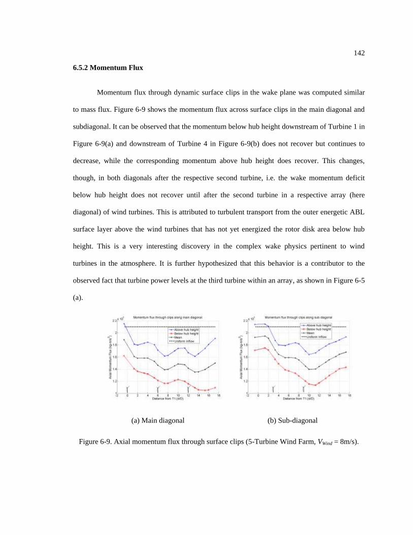
142

6.5.2 Momentum Flux

Momentum flux through dynamic surface clips in the wake plane was computed similar

to mass flux. Figure 6-9 shows the momentum flux across surface clips in the main diagonal and

subdiagonal. It can be observed that the momentum below hub height downstream of Turbine 1 in

Figure 6-9(a) and downstream of Turbine 4 in Figure 6-9(b) does not recover but continues to

decrease, while the corresponding momentum above hub height does recover. This changes,

though, in both diagonals after the respective second turbine, i.e. the wake momentum deficit

below hub height does not recover until after the second turbine in a respective array (here

diagonal) of wind turbines. This is attributed to turbulent transport from the outer energetic ABL

surface layer above the wind turbines that has not yet energized the rotor disk area below hub

height. This is a very interesting discovery in the complex wake physics pertinent to wind

turbines in the atmosphere. It is further hypothesized that this behavior is a contributor to the

observed fact that turbine power levels at the third turbine within an array, as shown in Figure 6-5

(a).


Figure 6-9. Axial momentum flux through surface clips (5-Turbine Wind Farm, VWind = 8m/s).

143

6.5.3 Power Density

The observation regarding the lagging of momentum recovery in the cross planes below

hub height and downstream of the first turbine in an array is further substantiated by analyzing

the actual power density [W/m2] through different surface clips. This is presented in Figure 6-10.

It is obvious that above hub height, the recovery in power density is fairly shallow after Turbine 1

in Figure 6-10(a) but progressively increases downstream of Turbine 2 and Turbine 3. This is

similar in Figure 6-10(b) for the subdiagonal array. This supports the thought that downward

momentum transport into the rotor disk area requires a long spatial distance in the ABL to

develop. Comparing Figures 6-10(a) and 6-10(b), it can be seen that Figure 6-10(b) shows a

nearly parallel recovery of power density after the second turbine in the sub-diagonal, while this

is not the case in Figure 6-10(a) for the main diagonal. This might support an idea of not placing a

third turbine in an array but instead letting the wake recover evenly for a longer distance before

placing an additional turbine.


Figure 6-10. Power density through surface clips (5-Turbine Wind Farm, VWind = 8m/s).

144

6.5.4 Turbulent Kinetic Energy

So far, we have analyzed mass and momentum fluxes and power density across surface

clips in wake planes and have studied the wake recovery. Now, it is worth discussing the TKE

across the surface clips. Figure 6-11 presents area averages of Turbulent Kinetic Energy (TKE)

through the cross-plane clips. The values shown in Figures 6-11 were averaged over 5 rotor

revolutions. It is best to interpret the plots shown in Figure 6-11 by looking at the mean (black

line) and differences between sub-areas above/below hub height. It is apparent that wind turbines

add TKE to the flow field. Unlike the observation in Figures 6-8, 6-9, and 6-10, it is interesting to

note, though, that the addition of TKE is similar above and below hub height, in contrast to the

momentum recovery in Figure 6-9. Furthermore, addition of TKE increases progressively for

downstream turbines, though the peak values in Figures 6-11(a) and 6-11(b) are almost identical.

This means that there seems to be a maximum possible TKE in a wind turbine array. The pattern

of rise and fall in TKE downstream of turbines in an array is consistent with the observations for

the turbine-turbine interaction problem in Figures 5-25 and 5-26 presented in chapter 5.


Figure 6-11. TKE through surface clips (5-Turbine Wind Farm, VWind = 8m/s).

145

6.6 Chapter Summary

This work presented a number of turbulence phenomena in the wakes of wind turbines

arranged in different arrays. A unique wake-plane integration analysis was used. It was

discovered that the lower portion of a cross plane lags behind in its recovery process by about 1

turbine spacing. The enhanced understanding of wake recovery pattern in a wind farm can help in

efficient planning of wind farm layouts. A comprehensive summary is presented in chapter 9.

146

Chapter 7

Actuator Curve Embedding-I: Development

It was shown in chapters 4 through 6 how the enhancement to the state-of-the-art ALM

affects the blade loads, integrated power, turbulence statistics, unsteadiness, and wake profile.

While the improvement and the ensuing study was a step ahead in advancing the state-of-the-art

in ALM, it was also noted that some limitations persist. Therefore, a more robust method to

model lifting surfaces is devised.

This chapter deals with the development of a method named actuator curve embedding

(ACE) that can model a general-shaped lifting surface (as a curve), either fixed or rotating. The

model is based on the most relevant physical parameter we are concerned with, i.e. the actual

blade/wing planform. This model could establish the reasoning outlined earlier that the Gaussian

spreading width, ε, be based on the actual planform such that the overlap of Gaussian spheres is

eradicated.

7.1 Persisting Issues with Actuator Line Method

It was mentioned earlier that the issue of overlap of the Gaussian spheres leads to an

over-prediction of blade tip loads. The overlap is shown by a schematic in Figure 7-1. It is thus

suggested that a method be devised such that the projection of blade forces on the volume grid

and the computation of volumetric forces using a kernel function do not have the issue of overlap.

This can be achieved if the kernel function is chosen in such a way that the projection of blade

forces is only in the disk region normal to the local blade section or the locus of actuator points.

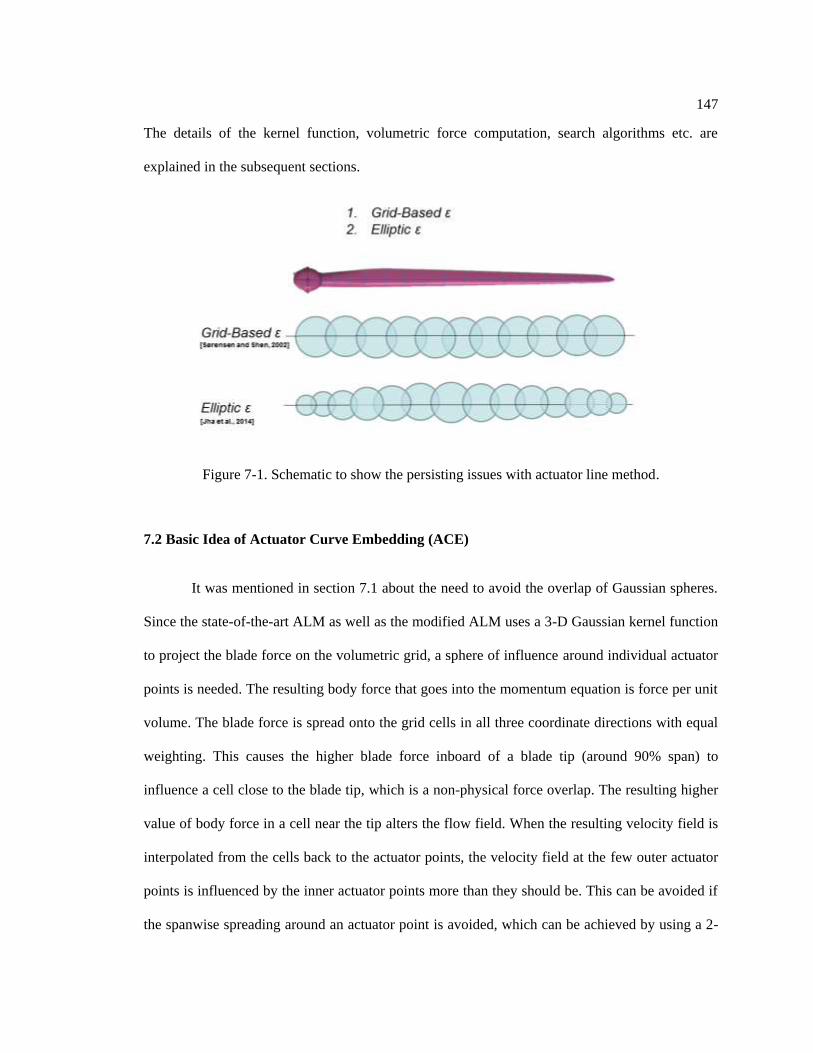
147

The details of the kernel function, volumetric force computation, search algorithms etc. are

explained in the subsequent sections.

Figure 7-1. Schematic to show the persisting issues with actuator line method.

7.2 Basic Idea of Actuator Curve Embedding (ACE)

It was mentioned in section 7.1 about the need to avoid the overlap of Gaussian spheres.

Since the state-of-the-art ALM as well as the modified ALM uses a 3-D Gaussian kernel function

to project the blade force on the volumetric grid, a sphere of influence around individual actuator

points is needed. The resulting body force that goes into the momentum equation is force per unit

volume. The blade force is spread onto the grid cells in all three coordinate directions with equal

weighting. This causes the higher blade force inboard of a blade tip (around 90% span) to

influence a cell close to the blade tip, which is a non-physical force overlap. The resulting higher

value of body force in a cell near the tip alters the flow field. When the resulting velocity field is

interpolated from the cells back to the actuator points, the velocity field at the few outer actuator

points is influenced by the inner actuator points more than they should be. This can be avoided if

the spanwise spreading around an actuator point is avoided, which can be achieved by using a 2-

148

D Gaussian kernel function. Here, the blade force computed at each of the actuator points along

the arc (or locus of actuator points) is spread in a disk normal to the local arc. The conservation of

blade and body force is taken care of by taking the actuator width into account. Moreover, instead

of looping over each actuator point and finding a sphere of influence around that actuator point,

and computing the contribution to body force in each cell in the sphere of influence, a reverse

approach is followed. Here, the entire flow field sees the influence of a blade/wing as a whole.

Some geometric properties are defined. The algorithm to accomplish this is explained in section

7.3. The 2-D Gaussian kernel function is explained in section 7.4. Once the entire flow field has

the information about how a blade is going to influence it, the blade force and the projected body

force can be computed. Each grid cell is associated with a unique actuator point on the curve

rather than visited by multiple actuator points, thus the issue of overlap is avoided. The

consideration of the entire curve at a time is illustrated in Figure 7-2. The idea of 3-D and 2-D

Gaussian kernel functions for ALM and ACE, respectively, is illustrated in Figure 7-3. The right

hand side of Figure 7-2 is an exaggerated view. In reality, the variation of local Gaussian

spreading width is much smoother as in Figure 7-3.

Figure 7-2. Schematic to illustrate the basic idea underlying actuator curve embedding (ACE).

149

Figure 7-3. Schematic to illustrate the 2-D Gaussian kernel function underlying the actuator curve

embedding (ACE).

7.3 Geometric Properties

Before explaining the methodology for ACE further, some geometeric parameters

associated with it are defined and tested on a small uniform grid. The turbine used for testing is

one with elliptic planform. The grid extent is 4R X 4R X 4R and the dimension is 80

X 80 X 80, resulting in a total of 512,000 cells with a grid resolution of R/20, where R is the

radius of the blade. The actuator width is chosen to be equal to the grid resolution, so that there

are 20 actuator points along the span in the baseline test case. The input parameters are chosen

such that, at the start of the simulation, the actuator points are coincident with the cell centroids

they lie in.

The different geometric parameters are illustrated in Figure 7-4. These parameters are

described in the following. The primitive or basic geometric parameters are named as ―pn‖, ―ps‖,

150

and ―fIndex‖. These are described via illustration in Figure 7-4. It is emphasized again that unlike

ALM, in ACE the entire blade is considered and seen by the flow field (cells) at a time instant.

While looping over each cell, the cell is assigned unique geometric properties depending on how

it sees the current blade under consideration. Unlike ALM where a cell can be influenced by

multiple actuator points and have cumulative effects, in ACE each cell is influenced by a unique

actuator point (―fIndex‖), which need not be a physical actuator point. The algorithm to determine

the unique geometric properties is presented in Appendix D but the key points are described here.

Figure 7-4. Schematic to illustrate the primitive geometric parameters associated with ACE.

For a given cell, a loop goes over all the actuator points of a blade that it sees at the

current time instant. For each actuator point pair m and m+1, the normal distance (―pn‖), and the

spanwise distance normalized by the local actuator width (―ps‖) are computed as illustrated in

Figure 7-4. The cell under consideration is said to be associated with the pair of actuator points

for which ―pn‖ is minimum. The fictitious actuator index that the cell is associated with is defined

151

as fIndex = m + ps. It can be noted from Figure 7-4 that two different cells can be associated with

the same pair of actuator points, m and m+1, but still have unique ―pn‖, ―ps‖, and ―fIndex‖.

The derived geometric parameters, defined for each cell, include the Gaussian spreading

width called ―epsLocal‖ and the coefficient of the Gaussian kernel function called ―etaField‖.

These will be explained and demonstrated in the forthcoming subsections.

(a) Algorithm for ACE

152

(b) Algorithm for ALM

Figure 7-5. Flow charts to illustrate the algorithm for ACE and its contrast with ALM.

A spanwise variation of Gaussian spreading width, ε, is provided as input. The Gaussian

spreading width at the fictitious actuator point, fIndex, is computed by interpolation of the values

at m-th and (m+1)-th actuator points. This is analogous to interpolation of blade loads from

physical actuator points to a fictitious one. For each cell for which the primitive geometric

parameters have been computed, the derived geometric parameters are computed based on

interpolated quantities at the fictitious actuator index, fIndex, associated with that cell. Once the

geometric parameters are computed, the algorithm for ACE can be completed. This is shown by a

flow chart in Figure 7-5.

153

7.3.1 Actuator Index Associated with Cells

As mentioned above, each cell is associated with a fictitious index for each of the blades.

At each time step and for each cell, the effect of each blade on that cell is computed by looping

over the blades and then accumulating the effect of all the blades. While looping over blades, the

geometric properties are computed afresh at the current time step. ―fIndex‖ is the index of the

fictitious actuator point on the current blade associated with the cell under consideration. Figure

7-6 shows a contour of the ―fIndex‖ in the rotor plane, and Figure 7-7 shows the ―fIndex‖ in a

horizontal plane through the rotor apex. These results are for a simulation with a single-bladed

rotor with elliptic planform. The intial position of the actuator curve (a line in this simple text

case) is also shown. The convention for the axes is the same as that for the ALM simulations, i.e.

an unconed rotor is in the y-z plane, and freestream flow is in the positive x-direction.

Figure 7-6. Contour plot of the basic geometric parameter ―fIndex‖ in the rotor plane.

154

It is obvious from these contour plots that the contour levels in the cells change as the

actuator index changes, hence suggesting that the actuator index that a cell is associated with is

computed correctly. All the cells cut through by a disk centered at an actuator point and normal to

the local arc have the same ―fIndex‖. It should also be noted that the geometric properties are not

computed beyond the sphere of influence of the rotor, which is centered at the intersection of

tower and rotor shaft. Overhang, the offset of rotor apex from tower-shaft intersection, is

illustrated in Figure 7-7. The basic geometric properties including ―fIndex‖ for cells lying to the

left of the first actuator point are the same as those of the cells associated with the first actuator

index. Similarly, the basic geometric properties of the cells lying to the right of the last actuator

point is same as that of the cells associated with the last actuator index.

Figure 7-7. Contour plot of the basic geometric parameter ―fIndex‖ in a horizontal plane through

the rotor apex.

7.3.2 Normal Distance

Similar to ―fIndex‖, ―pn‖, or the normal distance from a cell to the actuator curve, is a

primitive geometric parameter. It is illustrated in Figure 7-4. Figure 7-8 shows the contour of

155

―pn‖ in the rotor plane, Figure 7-9 shows ―pn‖ in a horizontal plane through the rotor apex, and

Figure 7-10 in a plane normal to the actuator curve at actuator index 1.

Figure 7-8. Contour plot of the basic geometric parameter ―pn‖ in the rotor plane.

Figure 7-9. Contour plot of the basic geometric parameter ―pn‖ in a horizontal plane through the

rotor apex.

It should be noted that the sphere of influence is centered at the intersection of tower and

shaft and not at the rotor apex; however, the normal distance is computed from the actuator curve,

156

which is hinged at the rotor apex (Figures 7-9 and 7-10). These contour plots suggest that the

basic geometric parameter ―pn‖ is computed correctly.

Figure 7-10. Contour plot of the basic geometric parameter ―pn‖ in a plane normal to the actuator

curve.

7.3.3 Spanwise Distance

The other component of the distance from a cell to the actuator point associated with it is

the normalized spanwise distance, ―ps‖ as illustrated in Figure 7-4. For a given cell, a value of

―ps‖ lying between 0 and 1 suggests that the actuator index it is associated with is between 1 and

Imax-1 where Imax is the highest actuator index. A negative ―ps‖ suggests that the cell lies to the left

of the first actuator point, and a value of ―ps‖ greater than 1 suggests that the cell lies to the right

of the highest actuator index. Once ―pn‖ and ―fIndex‖ have been computed, ―ps‖ is recomputed to

set it to either 0 or 1. If ―ps‖ is greater than or equal to 1, it is reset to 1, otherwise to 0. The

details of the algorithms are presented in Appendix D. Figure 7-11 shows a contour of ―ps‖ in the

157

rotor plane and Figure 7-12 shows ―ps‖ in a horizontal plane through the rotor apex. The

concurrence with the algorithm is apparent.

Figure 7-11. Contour plot of the basic geometric parameter ―ps‖ in the rotor plane.

Figure 7-12. Contour plot of the basic geometric parameter ―ps‖ in a horizontal plane through the

rotor apex.

158

7.3.4 Gaussian Distribution

The Gaussian spreading distance, ε, along the blade span, as described in chapter 4, is

now associated with the flow field because each cell is now associated with a fictitious actuator

point. The Gaussian spreading width at the fictitious actuator point, ―fIndex‖, is computed by

interpolation. For each cell for which the primitive geometric parameters have been computed,

―epsLocal‖ is computed based on the interpolated ε at ―fIndex‖ associated with that cell.

Figure 7-13 shows a contour plot of the derived geometric parameter ―epsLocal‖ in the

rotor plane and Figure 7-14 shows the ―epsLocal‖ in a horizontal plane through the rotor apex.

An elliptic variation of ―epsLocal‖ along the span is provided as input. Each cell sees ―epsLocal‖

at the ―fIndex‖ it is associated with. It is also obvious that all the cells cut through by a disk

normal to actuator arc have the same ―epsLocal‖, as expected.

Figure 7-13. Contour plot of the derived geometric parameter ―epsLocal‖ in the rotor plane.

159

Figure 7-14. Contour plot of the derived geometric parameter ―epsLocal‖ in a horizontal plane

through the rotor apex.

7.3.5 Eta field

The derived geometric parameter ―etaField‖ is finally computed as the net effect of the

Gaussian spreading width associated with a cell (―epsLocal‖) and the normal distance of this cell

from the actuator curve (―pn‖). Equation 7-1 shows the expresson for computed ―etaField‖. For

sake of simplicity, epsLocal is represented by ε in equation 7-1.

(7-1)

This is essentially the coefficient of blade force in using a 2-D Gaussian projection

function described in section 7.4. This is a measure of the effect in a cell, of the blade force

computed at the actuator point associated with that cell (―fIndex‖). This depends on ―epsLocal‖

associated with ―fIndex‖ and the normal distance from the actuator curve to the cell, ―pn‖. As the

distance grows, the effect of blade force in a cell decays rapidly. Moreover, the effect is only

along a disk normal to the local arc. There is no overlap between these disks.

160

Figure 7-15. Contour plot of the derived geometric parameter ―etaField‖ in the rotor plane.

Figure 7-16. Contour plot of the derived geometric parameter ―etaField‖ in a horizontal plane

through the rotor apex.

Figure 7-15 shows the contour of ―etaField‖ in the rotor plane, Figure 7-16 shows ―pn‖ in

a horizontal plane through the rotor apex, and Figure 7-17 in a plane normal to the actuator curve

at actuator index 1. The concentration of effect at the tips, due to smaller ―epsLocal‖ is visible.

The decay with ―pn‖ limits ―etaField‖ mostly in the vicinity of the actuator curve.

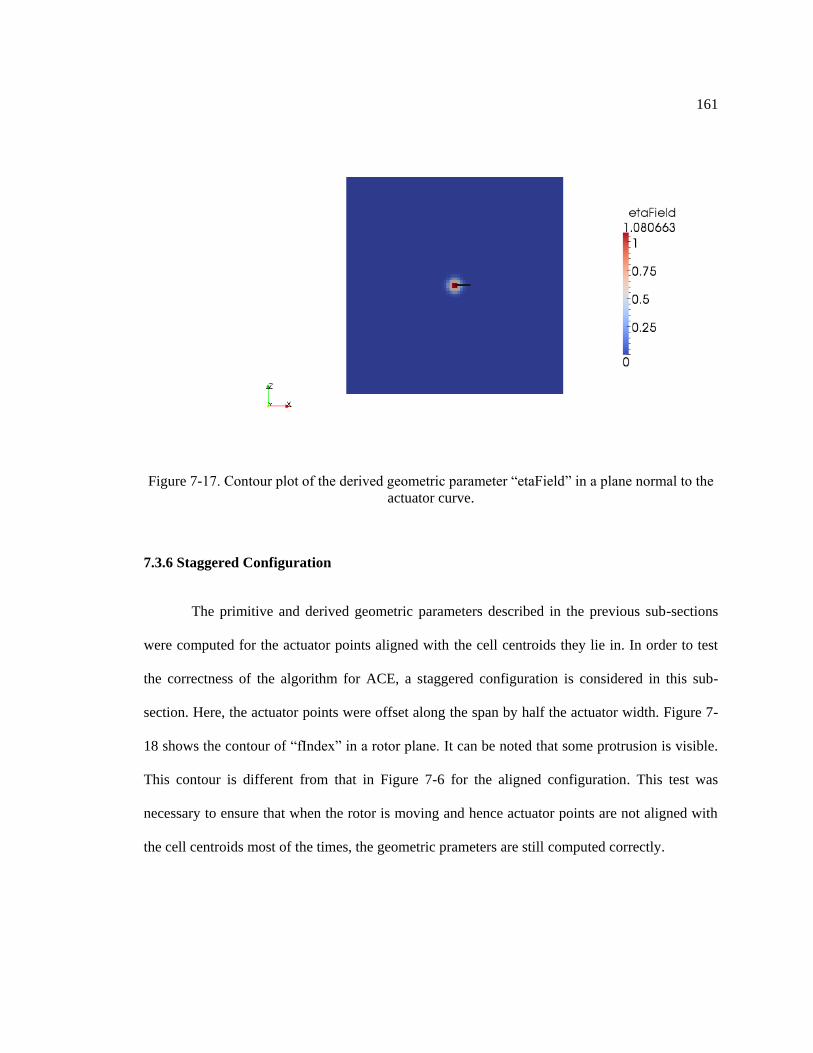
161

Figure 7-17. Contour plot of the derived geometric parameter ―etaField‖ in a plane normal to the

actuator curve.

7.3.6 Staggered Configuration

The primitive and derived geometric parameters described in the previous sub-sections

were computed for the actuator points aligned with the cell centroids they lie in. In order to test

the correctness of the algorithm for ACE, a staggered configuration is considered in this sub-

section. Here, the actuator points were offset along the span by half the actuator width. Figure 7-

18 shows the contour of ―fIndex‖ in a rotor plane. It can be noted that some protrusion is visible.

This contour is different from that in Figure 7-6 for the aligned configuration. This test was

necessary to ensure that when the rotor is moving and hence actuator points are not aligned with

the cell centroids most of the times, the geometric prameters are still computed correctly.

162

Figure 7-18. Contour plot of the basic geometric parameter ―fIndex‖ in the rotor plane for a

staggered configuration.

7.3.7 Rotated Actuator Curve

Apart from the staggered configuration, it is also important to ensure that the geometric

parameters are computed correctly for all azimuthal poitions of the actuator curve as the rotor is

moving. The results are presented in this sub-section for the rotor in a position rotated in the rotor

plane (y-z plane) by 45 degrees in the counter clockwise direction when viewed from behind the

rotor (downstream). Figure 7-19 shows the contour of primitive and derived geometric properties

in the rotor plane. These contour plots suggest the correct computation of geometric parameters

for the rotated actuator curve.

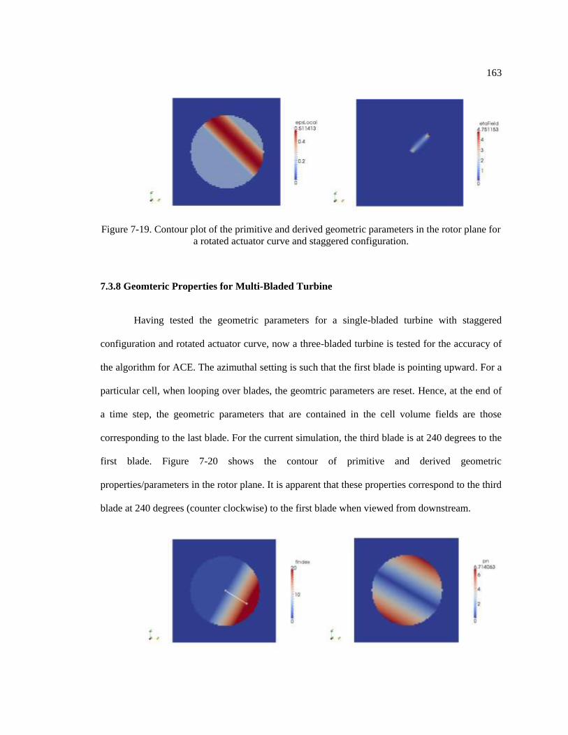
163

Figure 7-19. Contour plot of the primitive and derived geometric parameters in the rotor plane for

a rotated actuator curve and staggered configuration.

7.3.8 Geomteric Properties for Multi-Bladed Turbine

Having tested the geometric parameters for a single-bladed turbine with staggered

configuration and rotated actuator curve, now a three-bladed turbine is tested for the accuracy of

the algorithm for ACE. The azimuthal setting is such that the first blade is pointing upward. For a

particular cell, when looping over blades, the geomtric parameters are reset. Hence, at the end of

a time step, the geometric parameters that are contained in the cell volume fields are those

corresponding to the last blade. For the current simulation, the third blade is at 240 degrees to the

first blade. Figure 7-20 shows the contour of primitive and derived geometric

properties/parameters in the rotor plane. It is apparent that these properties correspond to the third

blade at 240 degrees (counter clockwise) to the first blade when viewed from downstream.

164

Figure 7-20. Contour plot of the primitive and derived geometric parameters in the rotor plane for

a three-blade turbine.

7.3.9 Transient Geomteric Properties for Multi-Bladed Turbine

In the previous three sub-sections, different possible scenarios of an actual rotating

turbine have been considered. The new algorithm for ACE must yield correct geometric

parameters for different azimuthal positions of the blade and for staggered configurations, and the

geometric properties must be reset after visiting each blade. These have been verified in the

previous three sub-sections. At this stage, an actual rotating turbine is simulated and the

geometric parameters are studied as the rotor moves, thereby changing azimuth and most of the

times being in staggered configuration.

At each time step, since the geometric parameters are reset and written to a volume field,

the geometric parameters are corresponding to the last blade. The transient simulations are

performed for a three-bladed turbine with 72 RPM and the first blade pointing upward. Figure 7-

21 shows the geometric parameter ―fIndex‖ for this simulation at different time instants. The

initial position of the third rotor is at 240 degrees counted counter-clockwise from the vertical

position.

165

t= 0.02 sec t= 0.04 sec t= 0.06 sec

t= 0.08 sec t= 0.10 sec

Figure 7-21. Contour plot of the basic geometric parameter ―fIndex‖ in the rotor plane for a three-

bladed turbine at different time instants.

7.4 Kernel Integration

The previous section described the computation of different geometric parameters

according to the algorithm for ACE presented in Appendix D. These geometric parameters are

used to compute the kernel function for projecting blade force onto the volumetric grid. The

computation of the body force for ACE implementation is different from that for the ALM

implementation. In order to avoid the overlap of the Gaussian, the spreading is done only in 2-D

normal to the local arc. This yields a force-per-unit-area term in projecting the blade force onto

the volumetric grid. The body force used in the momentum equation (analogous to the ALM) is

computed using equation 7-2.

∭ ( ) ∫ (∬( ∗ (

)

) ) (7-2)

166

Here, is the actuator width. The computation of geometric parameters and body force

to be used in the momentum equation is illustuated in Appendix D and is summarized below:

For each cell, loop over each blade and make the effect of individual blades cumulative

For a cell and the blade under consideration

find the set of actuator points with the shortest distance from the cell to the blade

(curve)

For the cell and blade pair, find the unique geometric parameters

Compute blade force at the modified actuator index

Compute body force at the cell by projecting the blade force computed using

Equation 7-2

• Each cell has cumulative effect of different blades, which is only the case close to the

blade root

t= 0.02 sec t= 0.04 sec t= 0.06 sec

t= 0.08 sec t= 0.10 sec

Figure 7-22. Contour plot of the magnitude of body force in the rotor plane for a three-blade

turbine at different time instants.

The above steps complete the description for representing the effect of turbines in the

flow field using the algorithm for ACE and without having the Gaussian overlap issues of ALM.

167

To conclude this section, results are presented for transient simulation for a three-bladed turbine

as in section 7.3.9, with kernel function implemented. Figure 7-22 shows the magnitude of the

computed ―bodyForce‖ (per unit volume) for this simulation at different time instants. The initial

position of the third rotor is at 240 degrees counter-clockwise from the vertical position.

7.5 Testing Different Curves

The real benefit of ACE is in applying this method to model an arbitrarily shaped lifting

surface (modeled as a curve), fixed or rotating. Therefore, testing this method for different types

of curves can assure its applicability to general-shaped lifting surfaces. The simplest case of a

straight line has already been presented in the previous section of kernel integration. In this

section, results for testing three different types of curves are presented. The first curve is a 2nd

order polynomial and the second is a 4th order polynomial

7.5.1 2nd

Order Polynomial

Figure 7-23. 2nd order polynomial for testing ACE.

-2 -1.5 -1 -0.5 0 0.5 1 1.5 2

-1.5

-1

-0.5

0

0.5

1

1.5

2

y

z

z = 0.1 y*2 + 0.0 y* + 0.0, y* = y-R/2

168

The 2nd order polynomial used ro represent a curved blade (could be due to aeroelasticity)

is

(

) (7-3)

Figure 7-23 shows the 2nd order polynomial used to test ACE. A transient simulation

similar to that in section 7.4 is performed with the straight rigid blades replaced by the 2nd order

polynomial and the first blade pointing in the positive y direction (azimuth = -90 degrees). Figure

7-24 shows the transient geometric parameter ―fIndex‖ at different time instants. Figure 7-25

shows the transient body force and Figure 7-26 shows the other geometric parameters, ―pn‖,

―epsLocal‖, and ―etaField‖, at t= 0.02 second.

t= 0.02 sec t= 0.04 sec t= 0.06 sec

t= 0.08 sec t= 0.10 sec


blade turbine at different time instants. The blade span is a 2nd order polynomial.

169

t= 0.02 sec t= 0.04 sec t= 0.06 sec

t= 0.08 sec t= 0.10 sec

Figure 7-25. Contour plot of the body force in the rotor plane for a three-blade turbine at different

time instants. The blade span is a 2nd order polynomial.

Figure 7-26. Contour plot of the geometric parameters in the rotor plane for a three-blade turbine

at t = 0.02 s. The blade span is a 2nd order polynomial.

7.5.2 4th

Order Polynomial

The 4th order polynomial used to represent a curved blade is:

(7-4)

where (

) (7-5)

170

Figure 7-27. 4th order polynomial for testing ACE.

Figure 7-27 shows the 4th order polynomial used to test ACE. Figure 7-28 shows the

transient geometric parameter ―fIndex‖ at different time instants. Figure 7-29 shows the transient

body force, and Figure 7-30 shows the other geometric parameters, ―pn‖, ―epsLocal‖, and

―etaField‖, at t= 0.02 second.

t= 0.02 sec t= 0.04 sec t= 0.06 sec

t= 0.08 sec t= 0.10 sec


blade turbine at different time instants. The blade span is a 4th order polynomial.

t= 0.02 sec t= 0.04 sec t= 0.06 sec

-2 -1.5 -1 -0.5 0 0.5 1 1.5 2

-1

-0.5

0

0.5

1

1.5

2

2.5

y

z

z = 0.02 y*4 + 0.03 y*

3 + 0.04 y*

2 + 0.05 y* + 0.06, y* = y-R/2

171

t= 0.08 sec t= 0.10 sec

Figure 7-29. Contour plot of the body force in the rotor plane for a three-blade turbine at different

time instants. The blade span is a 4th order polynomial.

Figure 7-30. Contour plot of the geometric parameters in the rotor plane for a three-blade turbine

at t = 0.02 s. The blade span is a 4th order polynomial.

7.6 Chapter Summary

This chapter presented the development of an actuator curve embedding method to model

a general-shaped lifting surface. The issues with using a 3-D Gaussian in the ALM were

addressed by using a Gaussian spreading normal to the local arc. This is accomplished by

defining several geometric parameters, computing kernel function using these parameters to

project the blade force onto the volumetric grid, and then implementing the effect of the turbine

or blade in the flow field as a body force. Different types of curves were tested to ascertain the

applicability of ACE to a general-shaped lifting surface modeled as a curve.

172

Chapter 8

Actuator Curve Embedding-II: Application

The details of the algorithm for ACE and several test cases including those for two

different curves were presented in chapter 7. This chapter deals with the application of ACE to

different types of rotors and operating conditions. Similar to the results presented in chapter 4

with state-of-the-art ALM and the improved ALM, here results are presented for the NREL Phase

VI rotor under rotating and parked conditions, elliptic wing, and the rotating NREL 5-MW

turbine. The operating conditions of the turbines and wing are the same as those in chapter 4.

The grid used for the simulations presented in this chapter has resolutions such that Δgrid

/R = 1/37 unless otherwise mentioned, so that comparisons can be made with the key results

presented in chapter 4 or results from similar simulations. The proposed guidelines for the

improved ALM require Δb/Δgrid to be greater than 1.5 to minimize the overlap of Gaussian

spheres. This puts a constraint on the maximum number of actuator points that can be used with

the improved ALM in chapter 4 for a given grid resolution. A benefit of using ACE is that this

constraint no longer exists, since there is no overlap of adjacent Gaussians. In principle, any

number of actuator points can be used. However, a reasonable number of actuator points that

yields good results for integrated quantities is around 40, without requiring much computational

resources. All the ACE simulations presented in this chapter were performed with 40 actuator

points.

A parameteric study of the spanwise distribution of Gaussian spreading width, which

follows the equivalent elliptic planform, is performed for the NREL phase VI rotor under roating

conditions. This parameteric study effectively means finding the ε/c* that yields the correct blade

173

loads, which are in turn dependent on the distribution of bound vortices. For all other simulations,

the results are presented for the ε/c* that yields correct blade loads.

8.1 NREL Phase VI Rotor: Rotating (72 RPM, Vwind = 7 m/s)

This section presents the results for the NREL Phase VI rotor under rotating conditions.

The wind speed is 7 m/s and the rotation speed of the rotor is 72 RPM. Firstly, a parametric study

is performed to find the Gaussian spreading width that yields correct blade loads. XTurb-PSU is

used for benchmarking the parametric study. Next, results are presented for ACE with the correct

distribution of Gaussian width. Comparisons are made with the results obtained with the state-of-

the-art as well as the improved ALM in chapter 4.

8.1.1 Parametric Study

The guidelines proposed in chapter 4 (section 4.6) for the improved ALM, especially for

the spanwise variation of Gaussian spreading width cannot be used as such for ACE. This is

because each actuator point represents a bound vortex element and its strength depends on the

local Gaussian spreading width. In ALM, there is interference between vortices resprented by

different actuator points. However, in ACE the interference is not there. The overall vorticity (due

to the rotor system as a whole) is conserved. This means the distribution of bound vortices along

the span is different from that in case of ALM, requiring a different distribution of Gaussian

spreading width.

A parameteric study for the chosen grid is presented in Figures 8-1, 8-2, and 8-3. The

spanwise distribution of Gaussian spreading width, ε, follows the equivalent elliptic planform.

The difference from ALM lies in the fact that the blade force is only spread normal to the blade

174

arc rather than in a spherical volume around the actuator point, which in turn is determined by the

Gaussian spreading width. Four different values of ε/c*, i.e. 0.3, 0.4, 0.5, and 0.6 are shown.

Figure 8-1 shows the AOA. Figure 8-2 shows the normal force coefficient and Figure 8-3 the

tangential force coefficient. It is observed that ε/c* = 0.4 results in very good comparison with the

XTurb-PSU results. It should be noted that ACE doesn‘t use any artificial tip correction.

Figure 8-1. Parametric study of spanwise variation of AOA for the rotating NREL Phase VI rotor

(Vwind = 7 m/s).

Figure 8-2. Parametric study of spanwise variation of normal force coefficient for the rotating

NREL Phase VI rotor (Vwind = 7 m/s).

175

Figure 8-3. Parametric study of spanwise variation of tangential force coefficient for the rotating

NREL Phase VI rotor (Vwind = 7 m/s).

8.1.2 Results

It is observed in the above sub-section that ε/c* = 0.4 yields the best comparison to blade

loads, in comparison to results obtained by XTurb-PSU. Figures 8-4, 8-5, and 8-6 show the

spanwise variation of AOA, normal force coefficient, and tangential force coefficient,

respectively. Comparions are made amongst the state-of-the-art ALM (grid based), the modified

ALM, ACE, XTurb-PSU, and the NREL data available for normal and tangential force

coefficients. It can be noted that the modified ALM as well as ACE predict tip loads well, without

using any artificial correction. However, the constraint on the number of actuator points is

alleviated by non-overlapping Gaussians along the span of the blade. This is expected to yield

more reliable integrated quantities, since a large number of actuator points can be used, even for a

coarse grid resolution. For the current case under consideration, the integrated power and thrust

are presented in Table 8-1. An improved comparison with NREL data and Xturb-PSU can be

observed.

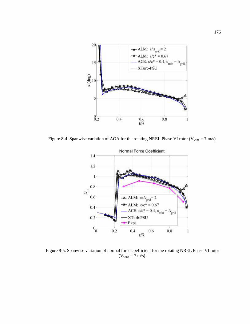
176

Figure 8-4. Spanwise variation of AOA for the rotating NREL Phase VI rotor (Vwind = 7 m/s).

Figure 8-5. Spanwise variation of normal force coefficient for the rotating NREL Phase VI rotor

(Vwind = 7 m/s).

177

Figure 8-6. Spanwise variation of tangential force coefficient for the rotating NREL Phase VI

rotor (Vwind = 7 m/s).

Table 8-1. Rotor power and thrust - NREL Phase VI rotor (Vwind = 7 m/s), Δgrid /R = 1/37.



XTurb-PSU 6,100 1,240

ALM (ε/Δgrid = 2.0, Δb /Δgrid = 1.0) 6,350 1,300

ALM (ε/c* = 0.67, Δb /Δgrid = 1.5) 6,210 1,280

ACE (ε/c* = 0.40) 6,150 1,250

8.2 NREL Phase VI Rotor: Parked (Vwind = 20.1 m/s)

This section presents the results for the NREL Phase VI rotor under parked condition.

The wind speed is 20.1 m/s and the pitch is 81.59 degrees. Results are presented for ACE with the

distribution of Gaussian width yielding correct blade loads. Comparisons are made with the

results obtained with the state-of-the-art ALM, the improved ALM, and XTurb-PSU as well as

the experimental data.

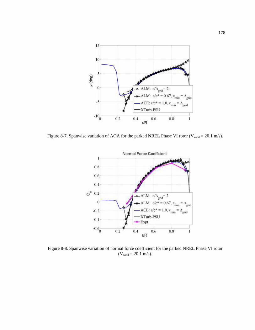
178

Figure 8-7. Spanwise variation of AOA for the parked NREL Phase VI rotor (Vwind = 20.1 m/s).

Figure 8-8. Spanwise variation of normal force coefficient for the parked NREL Phase VI rotor

(Vwind = 20.1 m/s).

179

Figure 8-9. Spanwise variation of tangential force coefficient for the parked NREL Phase VI rotor

(Vwind = 20.1 m/s).

It is observed that ε/c* = 1.0 yields the correct blade loads. Figures 8-7, 8-8, and 8-9

show the spanwise variation of AOA, normal force coefficient, and tangential force coefficient,

respectively. It can be noted that here also ACE predicts tip loads well, without using any

artificial correction. Moreover, there is no contstraint on the maximum number of actuator points.

It is also worth noting that the Gaussian spreading width along the span (represented by

ε/c*) is different from the case of the rotating NREL Phase VI rotor. This suggests that apart from

the blade geometry and grid that comprise parameters for the guidelines using the improved

ALM, wake rotation and freestream velocity may also affect the strength of the vortices and

hence the Gaussian spreading width, which represents the source of vortices at the actuator

points. This is recommended as a subject of future work.

180

8.3 Elliptic Wing

Results are presented for ACE with the distribution of Gaussian width yielding correct

blade loads. This is achieved for ε/c* = 0.7. Figure 8-10 shows the spanwise distribution of AOA

for the elliptic wing considered. Comparisons are made with the results obtained with the state-

of-the-art ALM, the improved ALM, and XTurb-PSU as well as the theory. It can be observed

that the issue of over-prediction of tip-loads is eradicated.

It should be noted that compared to the parked NREL Phase VI rotor, the twist along the

span and the rotor solidity (and induction factor) are different. These are the possible reasons for

the difference in the Guassian spreading width compared to the parked NREL Phase VI rotor,

since the equivalent elliptic planform and freestream velocity are the same in the two cases.

For the sake of completeness, tip vortices trailing from the elliptic wing are shown

qualitatively in Figure 8-11 and they augment the quantitative AOA in Figure 8-10.

Figure 8-10. Spanwise variation of AOA for the elliptic wing (Vwind = 20.1 m/s).

181

Figure 8-11. Tip vortices trailing from an elliptic wing modeled using ACE (Vwind = 20.1 m/s)

8.4 NREL 5-MW Turbine (9.16 RPM, Vwind = 8 m/s)

Having validated the actuator curve embedding algorithm for the NREL Phase VI rotor

and elliptic wing, it is now applied to the NREL 5-MW turbine, a conceptual utility-scale turbine.

The wind speed is 8 m/s, and the rotation speed of the rotor is 9.16 RPM. The grid used has

resolution Δgrid /R = 1/32. Results for ACE are presented for ε/c* = 1.2. Comparisons are made

with the results obtained with the state-of-the-art ALM, the improved ALM, and XTurb-PSU.

Experimental data are not available for this turbine. ACE simulations are also performed for a

Gaussian spreading width based on actual blade planform. This is done to assess the importance

of equivalent elliptic planform even for a turbine with equivalent elliptic planform being very

close to the actual planform, except near the blade tip. Figures 8-12, 8-13, and 8-14 show the

spanwise variation of AOA, normal force coefficient, and tangential force coefficient,

182

respectively. It can be observed that ACE results are very consistent with XTurb-PSU results. It

can also be observed that ACE with a Gaussian width based on elliptic planform performs better.

Figure 8-12. Spanwise variation of AOA for the rotating NREL 5-MW turbine (Vwind = 8 m/s).

Figure 8-13. Spanwise variation of normal force coefficient for the rotating NREL 5-MW turbine

(Vwind = 8 m/s).

183

A possible reason that the Gaussian spreading width requirement is very different from

that of the NREL Phase VI rotor is the wake advection rate (nearly the same for the two cases)

compared to the size of the domain (an order of magnitude difference). This reason is in addition

to other parameters such as planform (aspect ratio), wake rotation etc.

Figure 8-14. Spanwise variation of tangential force coefficient for the rotating NREL 5-MW

turbine (Vwind = 8 m/s).

8.6 Chapter Summary

This chapter was devoted to the application of ACE to different rotors and elliptic wing.

Its capability to model curves was tested in chapter 7. This makes ACE possibly suitable for

aeroelastic study of utility-scale turbines.

The Gaussian spreading width identified in the ACE simulation that yield correct blade

loads for different cases are:

NREL Phase VI (Rotating): ε/c* = 0.4

NREL Phase VI (Parked): ε/c* = 1.0

184

Elliptic wing: ε/c* = 0.7

NREL 5-MW turbine: ε/c* = 1.2

It was noted in the discussions that there could be several parameters determining the

Gaussian spreading width along the span, which would result in correct vorticity distribution and

hence the blade loads. These are:

Freestream velocity

Wake rotation

Twist along the span

Rotor solidity (and induction factor)

Wake advection rate

The results presented in this chapter and the parameters identified above make the ground

for further research into the development of ACE and its dependence on these parameters.

185

Chapter 9

Summary and Recommendations for Future

Research

This chapter presents a comprehensive summary of the work presented in previous

chapters and some recommendations for future research.

9.1 Summary

This dissertation started with an overview of the wind farm operations and the issue of

interest. This was followed by a detailed literature survey and previous work to model and

understand wind farm wakes. An outline of the work presented in this dissertation was discussed.

This was followed by the description of numerical tools to model atmospheric boundary layer,

turbine arrays, and a combination of the two. The accuracy of state-of-the-art ALM was assessed

by studying different rotor configurations under different operating conditions. It was found that

the standard ALM is grid-dependent and leads to over-prediction of blade tip-loads. Moreover, an

artificial tip correction is used to deal with this over-prediction. A new method implementing the

Gaussian spreading width based on equivalent elliptic planform was developed and validated.

This new method (ALM*) produced consistent results for different grid resolutions and rotors,

without using any artificial tip correction. Some general guidelines for using ALM* were

developed. Both ALM and ALM* were applied to a turbine-turbine interaction problem for two

ABL stability states. The differences in blade loads, integrated quantities, unsteadiness, and wake

profiles were quantified. The ALM* was then applied to an array of five NREL 5-MW turbines.

Recovery behavior of wakes using a unique wake-plane integration analysis was studied. This

186

improved understading can help in efficient planning of wind farms. Next, an actuator curve

embedding method to model a general-shaped surface as a lifting curve was developed. This was

validated for the NREL Phase VI rotor under rotating and parked conditions and an elliptic wing.

This was then applied to study the NREL 5-MW turbine. A comprehensive summary of the

different studies mentioned above is presented in the sub-sections below.

9.1.1 Accuracy Assessment and Improvement of Actuator-Line Modeling

The ALM within the ABL-LES solver is increasingly used as the evolving standard for

the computation of wake interactions in large wind farms. As of today, however, no general

guidelines exist for choosing ALM modeling parameters on LES-type grids. The main

contribution of this work is the development and testing of a much-needed set of guidelines to

determine the most important ALM parameters, i.e., the Gaussian radius ε, the grid resolution

Δgrid/R, and the actuator spacing Δb/Δgrid. An elliptic spanwise distribution of the Gaussian radius ε

is proposed along the blade where the equivalent elliptic planform c* has the same aspect ratio as

the actual blade. With reference to Schrenk‘s approximation used in the fixed-wing community,

this represents a first-order approximation of the actual blade loading and defines a constant value

for ε/c* along the blade that predominantly depends on the grid resolution and the blade aspect

ratio. This is essentially a more general way of representing tip loss.

The new set of guidelines for determining ALM parameters was tested for the NREL

Phase VI rotor and the NREL 5-MW turbine. For the NREL Phase VI rotor, it was first

demonstrated that the current best-practice of a grid-based Gaussian radius ε/Δgrid = constant leads

to an overprediction of blade tip loads; hence, rotor power and thrust are not necessarily correct.

Furthermore, the value of ε/Δgrid could be tuned to give the correct power and thrust, which are

integrated quantities, but the spanwise distribution of loading would not have the proper shape. A

187

recent idea of using a chord-based Gaussian radius ε/c = constant was also shown not to solve the

apparent issue of overpredicting blade tip loads for the NREL Phase VI rotor; however, there was

some improvement compared to the grid-based ε/Δgrid = constant. As for the proposed guidelines

that involve an elliptic Gaussian radius ε/c* = constant along the actuator line, good comparisons

were obtained against measured NREL data and results computed by the BEM-based XTurb-PSU

code using the same airfoil tables as the ALM simulations. Given the airfoil tables, the ALM

results obtained with the proposed guidelines are believed to be as close to measured NREL data

as the unmodified airfoil tables allow. It should be noted, though, that the NREL Phase VI rotor

blade has tips of finite chord (the rotor does not elliptically approach zero chord length at the tip);

however, it exhibits more of an elliptic-shaped loading. The ε/c = constant force projection

reflects the chord distribution and not the load distribution, so it is understandable that the method

is in error and highlights a common blade geometry upon which that method does not work as

well as the ε/c* = constant projection. For the NREL 5-MW turbine, no data are available, and

quantitative comparisons of ALM-computed blade loads along with rotor power and thrust were

performed against results obtained by the XTurb-PSU code. It was shown that the proposed

guidelines for ALM parameters rooted in an elliptic Gaussian radius ε/c* show consistent and

good results for blade loads as well as rotor power and thrust on various LES-type grids used in

large wind farm wake simulations.

In conclusion, the proposed guidelines for ALM parameters on LES-type grids have

proven to give consistent and good comparisons and thus provide the wind energy community

with a useful and much-needed methodology to model wind turbine wakes as accurately as

embedded airfoil data tables allow. The ALM computations for the NREL 5-MW turbine suggest,

however, that some future work is needed to provide a tighter criterion for equation 4-4 of this

work that relates the maximum spreading radius parameter to the grid spacing as the product nmax

Δgrid/R. It is surmised that application to other wind turbine rotors by the wind energy community

188

will provide more precise values for this product. The main contribution of this work has been to

develop and test the idea of an elliptic Gaussian radius along the blade span that accounts for a

consistent and correct distribution of blade loads along the actuator line.

9.1.2 Turbulence Statistics and Unsteadiness of Blade Loads for Turbine-Turbine

Interaction

While a lot of effort has been expended towards predicting wake velocity deficits and

turbulence statistics downstream of wind turbines and deep into large wind farms, little attention

has been given to predicting the spanwise blade loads of individual turbine blades and their local

response to variable atmospheric inflow conditions, and whether or not unsteady blade-section

aerodynamics is of importance. Also, the detailed study of Reynolds stresses and TKE has not

been carried out earlier.

The objective of this work was to assess how differences in two actuator-line methods

affect local as well as integrated turbine quantities such as the turbine power along with wake

velocity deficits and Reynolds stresses at various locations in the wake. Two atmospheric stability

states were considered, i.e. a neutral and a moderately-convective atmospheric boundary layer

representative of an offshore environment. The simulations were limited to an array of two NREL

5-MW wind turbines separated by seven rotor diameters. It was found that a difference (or

uncertainty) in mean turbine power of the order of 4 percent occurs as a result of the specific

actuator-line method. This difference was mainly attributed to a difference in local blade loads

outboard of the r/R = 0.85 spanwise blade station.

As such, for the first turbine in an array, the uncertainty between particular actuator-line

modeling approaches is of the same order as the variations associated with the atmospheric

stability state itself. This is potentially important for estimating blade fatigue and associated

189

operating and maintenence costs as well as array performance. An improved volumetric

projection method based on an equivalent elliptic chord distribution responds more sensitively to

unsteady inflow conditions near the blade tip, which is important to monitor the structural health

of the blades, yet it can only be validated with future field and/or highly-resolved hybrid RANS-

LES blade loads data. It should be noted that the best-practice values for parameter settings in

either ALM approach were used; more uncertainty is expected when deviating from these

recommended settings. These differences, starting with the local blade angle of attack outboard of

the r/R = 0.85 spanwise station, are propagated into the respective turbine wakes and are observed

in the wake deficits. This gives confidence that the underlying OpenFOAM LES solver does not

artificially (numerically) dissipate these differences. Furthermore, this work quantified, for the

first time, the importance of unsteady aerodynamic effects through a reduced frequency defined

by means of the rate-of-change of the sectional blade angle of attack. It is apparent now that

unsteady aerodynamics, currently not accounted for in the ALM table look-up procedure using

steady airfoil data, is of importance, particularly at inboard blade stations and downstream

turbines. The two ALM methods considered in this work differ in how important unsteady

aerodynamic effects are at outboard stations close to the blade tip. The two ALM methods,

however, do not differ much in terms of Reynolds stresses and TKE.

The true message of this work to the wind energy community is the following: an

uncertainty of only one percent in the performance of a large wind farm, for example the Horns

Rev wind farm in Denmark, can cost an operator more than one million dollars per year. While

the present work pushes the physical and accuracy limits of state-of-the-art actuator-line

modeling, there is a need for the wind energy community to quantify uncertainties for modeling

accuracy of wind farm wake models that account for unsteady aerodynamics at blade sections. It

is apparent that modeling accuracy is still not at a sufficient level, and the community of wind

energy researchers is tasked with both finding innovations to the current modeling techniques that

190

include unsteady aerodynamics but also to advance modeling fidelity on highly parallel

computing systems and defining needs for experimental data campaigns to validate the various

computational efforts.

9.1.3 Turbulence Transport Phenomena and Wake Recovery Pattern in a Wind Farm

This work presented a number of turbulence transport phenomena in the wakes of wind

turbines arranged in an array. The actuator line method (ALM) was used in an ALM

OpenFOAM-LES solver for all computations. The turbine model was that of the notional NREL

5-MW baseline turbine developed by NREL. The analyses included time series of turbine power,

wake momentum (velocity) deficits, turbulent kinetic energy (TKE) signifying wake turbulence

and wake meandering, and integrated surface fluxes enabled through post-processing. The

analyses presented in this work lead to the following conclusions:

The ABL stability state defines the shear in the atmospheric boundary layer (ABL)

and has a profound effect on the wake recovery and power production of wind

turbine arrays.

For wind farms arranged in staggered arrays, the downstream array is affected by the

wake of the upstream array, even for perfectly aligned wind conditions (zero yaw).

This leads to a small power loss in the (downstream) staggered array; however, the

standard deviation in power, and most probably fatigue loads, are reduced at a higher

rate compared to the power loss. This may be of interest for future array planning.

The observed fact from many wind farms that power production has leveled out by

the third turbine in an array has been confirmed in the computations of this work in

the example of a 5-turbine wind farm.

191

The use of the ‗dynamic surface clipping‘ method in FieldView allowed to separate

integrated fluxes of mass, momentum, power density, and Turbulent Kinetic Energy

(TKE) in wake surface cutting planes above and below hub height. It was discovered

that the lower portion of a wake surface cutting plane lags in its recovery process by

about 1 turbine spacing.

There are still many questions that are unanswered about the complex flow physics in

atmospheric flows and their interaction with wind turbines. This work showed how state-of-the-

art flow visualization combined with quantitative analyses is a promising means of unraveling the

remaining mysteries of wind turbine wakes.

9.1.4 Actuator Curve Embedding

An actuator curve embedding (ACE) method to model a general-shaped lifting surface

was developed and validated. The issues with using 3-D Gaussian in ALM were addressed by

using a Gaussian spreading normal to the local arc. A new force projection method using several

geometric parameters was developed. Different types of curves were tested to ascertain the

applicability of ACE to a general shaped lifting surface.

The ACE was applied to different rotors and elliptic wing. The capability of ACE to

model curves makes it suitable for aeroelastic studies of utility-scale turbines. Several parameters

such as freestream velocity, wake rotation, twist distribution along the blade span, and wake

advection rate etc. were identified, that possibly determine the Gaussian spreading width along

the span, which would result in correct vorticity distribution and hence the blade loads. This work

has prepared the ground for further research into the development of ACE and its dependence on

these parameters.

192

9.2 Future Research

This section describes some proposed research that could be performed on the basis of

the work presented in this dissertation.

9.2.1 Coupling Actuator Curve Embedding with a Structural Solver

The actuator curve embedding method (ACE) has been developed for a general-shaped

lifting surface (modeled as a curve). This makes it very suitable for simulating utility-scale wind

turbines with large flexible blades. A future research to couple ACE with a structural solver is

proposed. As the blade rotates through the flow field, it undergoes flap-wise and edge-wise

bending. It also experiences torsion. The physics of these phenomena is not modeled in the ACE

or ALM. Since ACE can model a general-shaped surface as a lifting curve, it is proposed that the

structural effects be incorporated at each time step of the simulation. At each time step, the ACE

algorithms would provide coordinates of the blade (and actuator points) and blade loads. Based

on these, the structural solver would compute the new bent and/or twisted position of the blade

until a convergence is achieved. The new coordinates of the flexible blade would then be used to

compute the blade loads again, which in turn, would be used to compute the new flow-field based

on two-way ACE-structural solver coupling. The ACE computation at the next time step would

then proceed with the modified flow-field.

9.2.2 Actuator Curve Embedding Applied to a Turbine Array

ACE has been validated for the NREL Phase VI rotor under rotating and parked

conditions, the NREL 5-MW turbine, and an elliptic wing, all in uniform inflow. A research that

could be performed is to apply ACE (with and without coupling with a structural solver) to a

193

turbine-turbine interation problem and a mini wind farm analogous to the studies presented in

chapters 5 and 6. A detailed study of the difference in prediction of blade loads, turbulence

statistics, unsteadiness, wake profiles, integrated power etc., by the two ALM methods and ACE,

is proposed. It is anticipated that ACE will perform better in predicting integrated quantities.

Application of ACE to actual wind farm such as Horns Rev. is also proposed.

9.2.3 Correlation between Blade Loads and Wake Parameters

It was noted in chapter 5 that the two ALM approaches showed noticeable difference in

the blade loads, turbulence statistics, integrated quantities, and unsteadiness. However, the

difference in wake profiles could not be ascertained. It is proposed that simulations be performed

for larger turbine arrays. The discrepancies in prediction of blade loads results in discrepancies in

prediction of the streangth of the tip vortices and their breakdown behavior and the subsequent

inflow to the downstream turbine. It is anticipated that far downstream in a row, the prediction of

wake profiles would be noticeably different using different approaches. In this regard, a detailed

study of the correlation between blade laods and wake profiles could shed some light on the

interdependence of blade loads (due to different actuator approaches) and the wake parameters

such as velocity deficit and Reynolds stresses.

9.2.4 Uncertainty Quantification in Wind Farm Modeling

The predictions of blade loads or wake parameters differ with the actuator approaches.

All these models attempt to represent the physics as closely as possible. However, each of these

models is based on certain assumptions that lead to some uncertainty in the results, apart from the

difference amongst themselves. It is proposed that a formal study of the uncertainty quantification

194

of the different actuator approaches be performed. In particular, the propagation of uncertainties

downstream in a row as well in lateral directions could be performed for a large wind farm such

as Horns Rev. This would provide answers to several physical questions about the operation of a

wind farm, modeling them using the aforesaid mathods, and the interaction between different

turbines.

195

References

1. Ammara, I., Leclerc, C., Masson, C., 2002. A Viscous Three-Dimensional

Differential/Actuator-Disk Method for the Aerodynamic Analysis of Wind Farms,

Journal of Solar Einergy Engineering, 124, 345-356.

2. Ainsle, J. J., 1988. Calculating the Flow in the Field of Wind Turbines, Journal of Wind

Engineering and Industrial Aerodynamics, 27, 213-224.

3. Barthelmie, R. J., Folkerts, L., Ormel, F., Sanderhoff, P., Eecen, P, Stobbe, O., Nielsen,

N. M., 2003. Offshore wind turbine wakes measured by SODAR, Journal of Atmospheric

and Oceanic Technology, 30, 466-477.

4. Barthelmie, R. J., and Coauthors, 2004. ENDOW (efficient development of offshore

wind farms): modeling wake and boundary layer interactions, Wind Energy, 7, 225-245.

5. Barthelmie, R. J., Folkerts, L., Rados, K., Larsen, G. C., Pryor, S., C., Frandsen, S.,

Lange, B., Schepers, G., 2006. Comparison of wake model simulations with offshore

wind turbine wake profiles measured by SODAR, Journal of Atmospheric and Oceanic

Technology, 33, 888-901.

6. Barthelmie, R. J., Frandsen, S. T., Nielsen, N. M., Pryor, S. C., Rethore, P. E., Jorgensen,

H. E., 2007. Modelling and measurements of power losses and turbulence intensity in

wind turbine wakes at Middelgrunden offshore wind farm, Wind Energy, 10, 217-228.

7. Barthelmie, R. J., Frandsen, S. T., Rethore, P. E., Jensen, L., 2007. Analysis of

atmospheric impacts on the development of wind turbine wakes at the Nysted wind farm,

Proceedings of the European Offshore Wind Conference, Berlin, Germany.

8. Barthelmie, R. J., Hansen, K., Frandsen, S. T., Rathmann, O., Schepers, J. G., Schlez, W.,

Phillips, J., Rados, K., Zervos, A., Politis, E. S., Chaviaropoulos, P. K., 2009. Modeling

196

and Measuring Flow and Wind Turbine Wakes in Large Offshore Wind Farms, Wind

Energy, 12, 431-444.

9. Barthelmie, R.J., Rathmann, O., Frandsen, S.T., Hansen, K., Politis, E., Prospathopoulos,

J., Rados, K., Cabezón, D., Schlez, W., Phillips, J., Neubert, N., Schepers, J.G., van der

Pijl, S.P, ―Modelling and measurements of wakes in large wind farms,‖ Journal of

Physics: Conference Series 75 (2007) 012049 doi:10.1088/1742-6596/75/1/012049

10. Bowen, A. J., Mortensen, N. G., 1996. Exploring the Limits of WAsP: The Wind

Analysis and Application Programme, Proceedings of the European Union Wind Energy

Conference, Gothenburg, Sweden.

11. Chevray, R., "The Turbulent Wake of a Body of Revolution", Journal of Basic

Engineering, pp. 275-284, June 1968

12. Churchfield, M. J., Moriarty, P. J., Vijayakumar, G., Brasseur, J., 2010. Wind Energy-

Related Atmospheric Boundary-Layer Large-Eddy Simulation Using OpenFOAM.

NREL/CP-500-48905.

13. Churchfield, M. J., 2011. Wind Energy / Atmospheric Boundary Layer Tools and

Tutorials. Training Session at the 6th OpenFOAM Workshop, The Pennsylvania State

University.

14. Churchfield, M. J., Li, Y., Moriarty, P. J., 2011. A Large-Eddy Simulation Study of

Wake Propagation and Power Production in an Array of Tidal-Current Turbines.

NREL/CP-5000-51765.

15. Conzemius, B., Lu, H., Chamorro, L., Wu, Y.-T., Porte-Agel, F., 2010. Development

and testing of a 21 wind farm simulator at an operating wind farm. Presentation from

AWEA 2010 WindPower Conference and Exhibition, Dallas, Texas.

197

16. Crespo, A., Hernandez, J., Fraga, E., Andreu, C., 1988. Experimental validation of the

UPM computer code to calculate wind turbine wakes and comparison with other models,

Journal of Wind Engineering and Industrial Aerodynamics, 27, 77-88.

17. Crespo, A., Hernandez, J., 1996. Turbulence Characteristics in Wind-Turbine Wakes,

Journal of Wind Engineering and Industrial Aerodynamics, 61, 71-85.

18. Dobrev, I., Massouh, F., Rapin, M., 2007. Actuator surface hybrid model. Journal of

Physics Conference Series, The Science of Making Torque from Wind, Technical

University of Denmark, Lyngby, Denmark.

19. Fletcher,T. M., and Brown, R.E., ‗‗Simulating Wind Turbine Interactions using the

Vorticity Transport Model,‘‘ 47th AIAA Aerospace Sciences Meeting , 5 - 8 January

2009, Orlando, Florida, AIAA 2009-838

20. L Hansen, K., Barthelmie, Cabezon, Politis (2008) UPWIND: Wake measurements used

in the model evaluation. UPWIND

21. Hassan, U. A., 1993. A Wind Tunnel Investigation of the Wake Structure within Small

Wind Turbine Farms, Rep. ETSU WN 5113.

22. Ivanell, S., Mikkelsen, R., Sorensen, J., Henningson, D., 2009. ACD Modelling of Wake

Interaction in the Horns Rev Wind Farm. In Extended Abstracts for Euromech Colloquim

508 on Wind Turbine Wakes, European Mechanics Society, Madrid, Spain.

23. Jensen, L. E., 2007. Analysis of array efficiency at Horns Rev and the effect of

atmospheric stability. EWEC Conference, Milan, Italy.

24. Jiminez, A., Crespo, A., Migoya, E., Garcia, J., 2007. Advances in Large-Eddy

Simulation of a Wind Turbine Wake. In The Science of Making Torque from Wind.

Conference Series, 75.

198

25. Johnson, C., 2008. Summary of actual versus predicted wind farm performance – a recap

of wind power 2008. Presentation from 2008 AWEA Wind Resource Assessment

Workshop, Portland, Oregon.

26. Katic, I., Hoejstrup, J., Jensen, N. O., 1986. A Simple Model for Cluster Efficiency,

Proceedings of the European Wind Energy Association, Rome, Italy.

27. Lange, B., Waldl, H., Guerrero, A. G., Heinemann, D., Barthelmie, R. J. 2003.Modeling

of Offshore Wind Turbine Wakes with the Wind Farm Program FLaP. Wind Energy, 6,

87-104.

28. Larsen, G. C., Carlen, I, Schepers, G. J., 1999. European Wind Turbine Standards 2.

Project Results, Rep. ECN-C-99-073 89.

29. Leclerc, C., Masson, C., 2004. Toward Blade-Tip Vortex Simulation with an Actuator-

Lifting Surface Model. AIAA-2004-0667.

30. Leclerc, C., Masson, C., 2005. Wind Turbine Performance Predictions Using a

Differential Actuator-Lifting Disk Model. J. Sol. Energ.Engin. Transactions of the

ASME, 127, 200-208.

31. Lu, H., and Porté-Agel, F., 2011, ―Large-Eddy Simulation of a Very Large Wind Farm in

a Stable Atmospheric Boundary Layer,‖ Phys. Fluids, 23, p. 065101.

32. Mann, J., 1994. The Spatial Structure of Neutral Atmospheric Surface-Layer Turbulence.

Journal of Fluid Mechanics, 273, 141-168.

33. Mann, J., 1998. Wind Field Simulation. Probabilistic Engineering Mechanics, 13, 269-

282.

34. Madsen, H. Aa., 1996. A CFD Analysis of the Actuator Disc Flow Compared With

Momentum Theory Results, Proceedings of the IEA Joint Action of Tenth Symposium on

Aerodynamics of Wind Turbines.

http://scitation.aip.org/content/aip/journal/pof2/23/6/10.1063/1.3589857

199

35. Magnusson, H., Rados, K. G., Voutsinas, S. G., 1996. A Study of the Flow Downstream

of a Wind Turbine Using Measurements and Simulations, Wind Engineering, 20(6), 389-

403.

36. Masson, C. Smaili, A., Leclerc, C., 2001. Aerodynamic Analysis of HAWTs Operating in

Unsteady Conditions, Wind Energy, 4, 1-22.

37. Masson, C, Ammara, I., Leclerc, C., and. Paraschivoiu, I. " Numerical simulations of the

three-dimensional turbulent flow in a wind park," AIAA-98-0058

38. Mechali, M., Jensen, L., Barthelmie, R., Frandsen, S., Rethore, P. E., 2006. Wake effects

at Horns Rev and their influence on energy production, Proceeding of the European Wind

Energy Conference and Exhibition, Athens, Greece.

39. Meyers. J., and Meneveau, C., 2010, ―Large Eddy Simulations of large wind-turbine

arrays in the atmospheric boundary layer,‖ AIAA-2010-827.

40. Mikkelsen, R., 2003. Actuator Disc Methods Applied to Wind Turbines. Technical

University of Denmark, PhD Thesis.

41. OpenFOAM – The Open Source CFD Toolbox, Programmer‘s Guide, Version1.6. Open

CFD Ltd., 9 Albert Road, Caversham, Reading, Berkshire RG4 7AN, UK.

42. OpenFOAM – The Open Source CFD Toolbox, User‘s Manual, Version1.6. Open CFD

Ltd., 9 Albert Road, Caversham, Reading, Berkshire RG47AN, UK.

43. Quarton, D., Ainsle, J., 1990. Turbulence in Wind Turbine Wakes, Wind Engineering, 14,

15-23.

44. Rados, K., Larsen, G., Barthelmie, R., Schlez, W., Lange, B., Schepers, G., Hegberg, T.,

Magnusson, M., 2002. Comparison of wake models with data from offshore wind farms,

Wind Engineering, 25, 271-280.

http://arc.aiaa.org/doi/abs/10.2514/6.2010-827

200

45. Rathmann, O., Frandsen, S. T., Barthelmie, R. J., 2007. Wake Modelling for Intermediate

and Large Wind Farms, Proceedings of the European Wind Energy Conference and

Exhibition, Milan, Italy.

46. Rethore, P. E., Sørensen, N. N., Zahle, F., 2010. Validation of an Actuator Disc Model,

EWEC 2010.

47. Sanderse, B., " Aerodynamics of wind turbine wakes," Energy Research Center of the

Netherlands report, ECN-E--09-016

48. Schepers, J. G., 1998. Wakefarm, Nabij zog model en ongestood windsnelheisveld (in

Dutch), Rep. ECN-C—98-016.

49. Schlez, W., Umana, A. E., Barthelmie, R., Larsen, S., Rados, K., Lange, B., Schepers, G.,

Hegberg, T., 2002. ENDOW: Improvement of wake models within offshore wind farms,

Wind Engineering, 25, 281-287.

50. Schlez, W., Umana, A., Barthelmie, R., Larsen, G., Rados, K., Lange, B., Schepers, G.,

Hegberg, T., 2001. ENDOW: Improvement of Wake Models within Offshore Wind

Farms. In Proceedings EWEC 2007.

51. Schmitz, S., Bhagwat, M., Caradonna, F. X., 2009. A Generalized Potential Method for

Modeling Rotor Wake Flows, AIAA-2009-3856.

52. Shen, W. Z., Zhang, J. H., Sorensen, J. N., 2009. The Actuator Surface Model: A New

Navier-Stokes Based Model for Rotor Computations. J. Sol. Energy Eng. Trans. ASME,

131(1), doi:10.1115/1.3027502.

53. Sibuet Watters, C., Masson, C., 2010. Modelling of Lifting-Device Aerodynamics Using

the Actuator Surface Concept. Int. J. Numer. Meth. Fl., 62(11), 1264-1298.

54. Singer, M., Mirocha, J., Lundquist, J., Cleve, J., 2010. Implementation and assessment of

turbine wake models in the Weather Research and Forecasting model for both mesoscale

and large-eddy simulation.

201

55. Sørensen, J. N., Shen, W. Z., Munduate, X., 1998. Analysis of Wake States by a Full-

Field Actuator Disc Model. Wind Energy. Int. J. Numer. Meth. Fl., 1, 73-78.

56. Sørensen, J. N., Shen, W. Z., 2002. Numerical modeling of Wind Turbine Wakes. J

Fluids Engineering, 124, 393-399.

57. Sørensen, J. N., Shen, W. Z., Munduate, X., 1998. Analysis of Wake States by a Full-

Field Actuator Disc Model. Wind Energy, 1, 73-88

58. Stovall, T. D., Pawlas, G., Moriarty, P. J., 2010. Wind farm wake simualtions in

OpenFOAM. AIAA-2010-0825.

59. Stull, R. B., 1988. An Introduction to Boundary Layer Meteorology. Kluwer Academic

Publishers, ISBN 10: 9027727694

60. Troen, I., Petersen, E. L., 1989. European Wind Atlas. Risoe National Laboratory for

Sustainable Energy, Roskilde, Denmark.

61. Troldborg, N., Sørensen, J. N., Mikkelsen, R., 2007. Actuator Line Simulation of Wake

of Wind Turbine Operating in Turbulent Inflow. Journal of Physics: Conference Series,

The Science of Making Torque from Wind, Technical University of Denmark, Lyngby,

Denmark.

62. Troldborg, N., 2008. Actuator Line Modeling of Wind Turbine Wakes, Technical

University of Denmark, PhD Thesis.

63. Troldborg, N., Sørensen, J., Mikkelsen, R., 2010. Numerical Simulations of Wake

Characteristics of a Wind Turbine in Uniform Flow. Wind Energy, 13, 86-99.

64. Troldborg, N., Sorensen, J.N., and Mikkelsen, R., "Actuator Line Simulation of Wake of

Wind Turbine Operating in Turbulent Inflow," Journal of Physics: Conference Series 75

(2007) 012063 doi:10.1088/1742-6596/75/1/012063

65. Veers, P. S., 1988. Three-Dimensional Wind Simulation. Technical Report SAND88-

0152, Sandia National Laboratories.

202

66. Vermeer, L. J., Soerensen, J. N., Crespo, A. 2003. Wind Turbine Wake Aerodynamics.

Progress in Aerospace Sciences, 39, 467-510.

67. Vermeulen, P. E. J., 1980. An Experimental Analysis of Wind Turbine Wakes,

Proceedings of the 3rd Symposium on Wind Energy Systems, 431-450.

68. WAsP – The Wind Atlas Analysis and Application Program. Risoe National Laboratory

for Sustainable Energy, Roskilde, Denmark. [Online]. Available:

http://www.wasp.dk/Products/WAsP.html (Accessed July 17th 2011)

69. Wharton, S. and J. K. Lundquist, 2010: Atmospheric stability impacts on power curves of

tall wind turbines — an analysis of a west coast north amer- ican wind farm. Technical

report, Lawrence Liver-more National Laboratory (LLNL), lLNL-TR-424425, https://e-

reports-ext.llnl.gov/pdf/387609.pdf.

70. Wolton, P.R., ―Wind farm wake prediction using CFD,‖ M.S. thesis, Mechanical

Engineering, University of Colorado at Boulder, 2008

71. Zahle, F., Soerensen, N. N., 2007. On the Influence of Far-Wake Resolution on Wind

Turbine Flow Simulations. In The Science of Making Torque from Wind. Conference

Series, 75.

72. Lavely, A.W., et al. Space-Time Loadings on Wind Turbine Blades Driven by

Atmospheric Boundary Layer Turbulence. in Proc. 49th AIAA Aerospace Sciences

Meeting, AIAA Paper 2011-635. 4-7 Jan 2011.

73. Segalini, A., and Alfredsson, P.H., 2013, ―A simplified vortex model of propeller and

wind-turbine wakes,‖ J. Fluid Mech., 725, pp. 91-116. doi:10.1017/jfm.2013.182

74. Okulov, V.L., and Sørensen, J.N., 2010, ―Maximum efficiency of wind turbine rotors

using Joukowsky and Betz approaches,‖ J. Fluid Mech., 649, pp. 497–508.

doi:10.1017/S0022112010000509

http://www.wasp.dk/Products/WAsP.html

https://e-reports-ext.llnl.gov/pdf/387609.pdf

https://e-reports-ext.llnl.gov/pdf/387609.pdf

http://journals.cambridge.org/action/displayAbstract?fromPage=online&aid=8912663&fileId=S0022112013001821


203

75. Calaf, M., Meneveau, C., and Meyers. J., 2010, ―Large eddy simulation study of fully

developed wind-turbine array boundary Layers,‖ Phys. Fluids, 22, 015110. doi:

10.1063/1.3291077

76. Meyers. J., and Meneveau, C., 2012, ―Optimal turbine spacing in fully developed wind

farm boundary layers,‖ Wind Energy, 15, pp. 305–317. DOI: 10.1002/we.469

77. VerHulst, C. and Meneveau, C., 2014, ―Large eddy simulation study of the kinetic energy

entrainment by energetic turbulent flow structures in large wind farms,‖ Phys. Fluids, 26,

025113. doi: 10.1063/1.4865755

78. Nathan, J., Bautista, M., Masson, C., and Dufresne, L., 2014, ―Study of the near wake of

a wind turbine in ABL flow using the actuator line method,‖ J. Physics: Conf. Ser., 524,

012141. doi:10.1088/1742-6596/524/1/012141

79. Okulov, V.L, and Sørensen,J.N, 2007, ―Stability of helical tip vortices in a rotor far

wake,‖ J. Fluid Mech., 576, pp. 1–25. doi:10.1017/S0022112006004228

80. Viola, F., Iungo, G. V., Camarri, S., Porté-Agel, F., and Gallaire, F., 2014, ―Prediction of

the hub vortex instability in a wind turbine wake: stability analysis with eddy-viscosity

models calibrated on wind tunnel data,‖ J. Fluid Mech., 750, R1,

doi:10.1017/jfm.2014.263

81. Hong, J., Toloui, M., Chamorro, L.P., Guala, M., Howard, K., Riley, S.,Tucker, J., and

Sotiropoulos, F., 2014, ―Natural snowfall reveals large-scale flow structures in the wake

of a 2.5-MW wind turbine,‖ NATURE COMMUNICATIONS, 5, 4216. DOI:

10.1038/ncomms5216

82. Chatelain, P., Backaert, S., Winckelmans, G., and Kern, S., 2013, ―Large Eddy

Simulation of Wind Turbine Wakes,‖ Flow Turbulence Combust, 91 (3), pp. 587–605.

DOI 10.1007/s10494-013-9474-8

http://scitation.aip.org/content/aip/journal/pof2/22/1/10.1063/1.3291077?ver=pdfcov

http://onlinelibrary.wiley.com/doi/10.1002/we.469/full/

http://scitation.aip.org/content/aip/journal/pof2/26/2/10.1063/1.4865755

http://journals.cambridge.org/download.php?file=%2FFLM%2FFLM576%2FS0022112006004228a.pdf&code=0d85ef12cc544ae34786ecfec8f757c2


http://www.nature.com/ncomms/2014/140624/ncomms5216/full/ncomms5216.html

http://link.springer.com/article/10.1007/s10494-013-9474-8

204

83. Stevens, R.J.A.M., Graham, J., and Meneveau, C., 2014, ―A concurrent precursor inflow

method for Large Eddy Simulations and applications to finite length wind farms,‖

Renewable Energy, 68, pp. 46-50. doi: 10.1016/j.renene.2014.01.024

84. Leishman, J.G., 2002, ―Challenges in modelling the unsteady aerodynamics of wind

turbines,‖ Wind Energy, 5, pp. 85–132. doi: 10.1002/we.62

85. Smagorinsky, J., 1963, ―General Circulation Experiments with the Primitive Equations,‖

Monthly Weather Review, 91, pp. 99-164.

86. R.B. Stull, 2000, ―Meteorology for Scientists and Engineers,‖ 2nd ed., Brooks/Cole,

Florence, KY.

87. R.B. Stull, 2009, ―An Introduction to Boundary Layer Meteorology,‖ Springer Science +

BusinessMedia B.V., Dordrecht Netherlands.

88. C.H. Moeng, 1984, ―A large-eddy simulation model for the study of planetary boundary

layer turbulence,‖ J. Atmos. Sci. 41, pp. 2052–2062.

89. D. Etling, Chapter 2, 1996 in ―Modelling of Atmospheric Flow Fields,‖ International

Atomic Energy Agency, Vienna, Austria, pp. 54–58.

90. Issa, R. I., 1985, ―Solution of the Implicitly Discretized Fluid Flow Equations by

Operator-Splitting,‖ Journal of Computational Physics, 62, pp. 40–65.

91. Rhie, C. M., and Chow W. L., 1983, ―Numerical Study of the Turbulent Flow Past an

Airfoil with Trailing Edge Separation,‖ AIAA Journal, 21 (11), pp. 1525–1532.

92. Wesseling, P., 2001, ―Elements of Computational Fluid Dynamics,‖ Lecture Notes

WI4011 TU Delft.

93. Martínez, L. A., Leonardi, S., Churchfield, Matthew J., and Moriarty, Patrick J., 2012, ―A

Comparison of Actuator Disk and Actuator Line Wind Turbine Models and Best

Practices for Their Use,‖ AIAA 2012-0900.

http://www.sciencedirect.com/science/article/pii/S0960148114000536

http://dx.doi/

http://onlinelibrary.wiley.com/doi/10.1002/we.62/abstract

205

94. Shives, M., and Crawford, C., 2012 ―Mesh and Load Distribution Requirements for

Actuator Line CFD Simulations,‖ Wind Energy, Vol. 15.

95. Schmitz, S., ―XTurb-PSU: A Wind Turbine Design and Analysis Tool,‖

http://www.aero.psu.edu/Faculty_Staff/schmitz/XTurb/XTurb.html

96. Jha, P. K., Brillembourg, D., and Schmitz, S., ―Wind Turbines under Atmospheric Icing

Conditions - Ice Accretion Modeling, Aerodynamics, and Control Strategies for

Mitigating Performance Degradation,‖ AIAA 2012-1287-868, 2012.

97. Moriarty, P.J., and Hansen, A.C., ―AeroDyn Theory Manual,‖ NREL/TP-500-36881,

January 2005, URL: http://www.nrel.gov/docs/fy05osti/36881.pdf.

98. Chattot, J.J., ―Design and Analysis of Wind Turbines Using Helicoidal Vortex

Model,‖ Computational Fluid Dynamics Journal, Vol. 11, No. 1, April 2002, pp. 50-54.

99. Du, Z., and Selig, M.S., ―A 3-D Stall-Delay Model for Horizontal Axis Wind Turbine

Performance Prediction,‖ AIAA 98-0021, 36th AIAA Aerospace Sciences Meeting and

Exhibit, 1998; ASME Wind Energy Symposium, Reno, NV, USA, January 12-15, 1998.

100. Hansen, C., AirfoilPrep, NWTC Design Code, Ver. 2.0, [available online]

National Renewable Energy Laboratory, Golden, CO, 2005, URL:

http://wind.nrel.gov/designcodes/preprocessors/airfoilprep/ [last modified 9 March 2010,

accessed December 7 2012].

101. Glauert, H., Airplane Propellers, Dover, New York, 1985, pp. 251-268.

102. Shen, W. Z., Zhu, W. J., and Sørensen, J. N., ―Actuator Line/Navier-Stokes

Computations for the MEXICO Rotor: Comparison with Detailed Measurements,‖ Wind

Energy, Vol. 15, No. 5, July 2012, pp. 811-825.

103. Shen, W. Z., Mikkelsen, R., Sørensen, J. N., and Bak, C., ―Tip Loss Corrections

for Wind Turbine Computations,‖ Wind Energy, Vol. 8, No. 4, October 2005, pp. 457-

475.

http://www.aero.psu.edu/Faculty_Staff/schmitz/XTurb/XTurb.html

http://arc.aiaa.org/doi/pdf/10.2514/6.2012-1287

http://www.nrel.gov/docs/fy05osti/36881.pdf

http://wind.nrel.gov/designcodes/preprocessors/airfoilprep/

206

104. Shen, W. Z., Sørensen, J. N., and Mikkelsen, R., ―Tip Loss Corrections for

Actuator/Navier-Stokes Computations,‖ ASME Journal of Solar Energy Engineering,

Vol. 127, No. 2, April 2005, pp. 209-213.

105. Jonkman, J., Butterfield, S., Musial, W., and Scott, G., ―Definition of a 5-MW

Reference Wind Turbine for Offshore System Development,‖ National Renewable

Energy Laboratory, NREL/TP-500-38060, Feb. 2009.

106. Schrenk, O., ―A Simple Approximation Method for Obtaining the Spanwise Lift

Distribution,‖ NACA TM No. 948, 1940.

107. Hand, M. M., Simms, D. A., Fingersh, L. J., Jager, D. W., Cotrell, J. R., Schreck,

S., and Larwood, S. M., ―Unsteady Aerodynamics Experiment Phase VI: Wind Tunnel

Test Configurations and Available Data Campaigns,‖ Rep. NREL/TP-500-29955, Dec.

2001.

108. Jha, P. K., Churchfield, M. J., Moriarty, P. J., and Schmitz, S., ―Accuracy of

State-of-the-Art Actuator-Line Modeling for Wind Turbine Wakes,‖ AIAA 2013-0608,

2013.

109. Schmitz, S., and Chattot, J. J., ―A Parallelized Couple Navier-Stokes/Vortex-

Panel Solver,‖ ASME Journal of Solar Energy Engineering, Vol. 127, No. 4, 2005, pp.

475–487.

110. Intelligent Light, http://www.ilight.com, Last accessed: April 03, 2014

111. Schmitz, Sven, ―AERSP 583, Wind Turbine Aerodynamics: Lecture Notes‖

http://arc.aiaa.org/doi/pdf/10.2514/6.2013-608

207

Appendices

Appendix A: MATLAB code to compute equivalent elliptic planform

clc; clear; close all;

inputFile = load('5MW_BladeData.txt');

outputFile = '5MW_BladeData_Fic.txt';

%R = ; % m, Phase VI

R = 63; % m, 5-MW

% Dimensionalize

r = inputFile(:,1);

chord = inputFile(:,2);

r = [0; r; R]

chord = [chord(1); chord; chord(length(chord))];

% Compute Area and Aspect Ratio of the Extrapolated blade

A_planform = trapz(r, chord);

AR_blade = R^2/A_planform;

% Ellipse

a = R/2.0; % Semi-major axis

AR_ellip = AR_blade; % Keep the same AR as the extrapolated blade....

A_ellip = R^2/AR_ellip;

b = 2*R/pi/AR_ellip;

% b = A_ellip/pi/a; % Both give the same answer

x = r;

y = b*sqrt(1 - (x/a -1).^2);

chord_ellip = 2*y;

bladeData_OpenFOAM = [inputFile(:,1) inputFile(:,2) chord_ellip(2:length(chord_ellip)-1)

inputFile(:,3) inputFile(:,4)];

dlmwrite(outputFile,bladeData_OpenFOAM,'delimiter','\t','precision','%8.4f %8.4f %8.4f %8.4f %d');

figure (1);

set(gca, 'FontSize',18);

plot(r,0.25*chord,'-or','LineWidth',2); hold on; grid on;

plot(x,y-0.25*b,'b','LineWidth',4);

plot(r,-0.75*chord,'-or','LineWidth',2);

plot(x,-y-0.25*b,'b','LineWidth',4);

xlabel('r (m)'); ylabel('c (m)'); title('Blade Planform');

axis('equal')

legendText2 = sprintf('Elliptic, A = %.3f m^2, AR = %.3f', A_ellip, AR_ellip);

legend('Original Planform',legendText2);

figure (2);

set(gca, 'FontSize',18);

plot(r/R,0.25*chord,'-or','LineWidth',2); hold on; grid on;

plot(x/R,y-0.25*b,'b','LineWidth',4);

plot(r/R,-0.75*chord,'-or','LineWidth',2);

plot(x/R,-y-0.25*b,'b','LineWidth',4);

xlabel('r/R'); ylabel('c (m)'); title('Blade Planform');

legendText2 = sprintf('Elliptic, A = %.3f m^2, AR = %.3f', A_ellip, AR_ellip);

legend('Original Planform',legendText2);

dummy = 0;

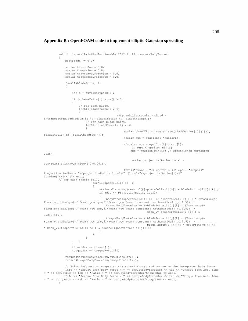
208

Appendix B : OpenFOAM code to implement elliptic Gaussian spreading

void horizontalAxisWindTurbinesALM_2012_11_18::computeBodyForce()

{

bodyForce *= 0.0;

scalar thrustSum = 0.0;

scalar torqueSum = 0.0;

scalar thrustBodyForceSum = 0.0;

scalar torqueBodyForceSum = 0.0;

forAll(bladeForce, i)

{

int n = turbineTypeID[i];

if (sphereCells[i].size() > 0)

{

// For each blade.

forAll(bladeForce[i], j)

{

//DynamicList<scalar> chord =

interpolate(bladeRadius[i][j], BladeStation[n], BladeChord[n]);

// For each blade point.

forAll(bladeForce[i][j], k)

{

scalar chordFic = interpolate(bladeRadius[i][j][k],

BladeStation[n], BladeChordFic[n]);

scalar eps = epsilon[i]*chordFic;

//scalar eps = epsilon[i]*chord[k];

if (eps < epsilon_min[i])

eps = epsilon_min[i]; // Dimensioned spreading

width

scalar projectionRadius_local =

eps*Foam::sqrt(Foam::log(1.0/0.001));

Info<<"Chord = "<< chordFic <<" eps = "<<eps<<"

Projection Radius = "<<projectionRadius_local<<" (local)"<<projectionRadius[i]<<"

Turbine["<<i<<"]"<<endl;

// For each sphere cell.

forAll(sphereCells[i], m)

{

scalar dis = mag(mesh_.C()[sphereCells[i][m]] - bladePoints[i][j][k]);

if (dis <= projectionRadius_local)

{

bodyForce[sphereCells[i][m]] += bladeForce[i][j][k] * (Foam::exp(-

Foam::sqr(dis/eps))/(Foam::pow(eps,3)*Foam::pow(Foam::constant::mathematical::pi,1.5)));

thrustBodyForceSum += (-bladeForce[i][j][k] * (Foam::exp(-

Foam::sqr(dis/eps))/(Foam::pow(eps,3)*Foam::pow(Foam::constant::mathematical::pi,1.5))) *

mesh_.V()[sphereCells[i][m]]) &

uvShaft[i];

torqueBodyForceSum += ( bladeForce[i][j][k] * (Foam::exp(-

Foam::sqr(dis/eps))/(Foam::pow(eps,3)*Foam::pow(Foam::constant::mathematical::pi,1.5))) *

bladeRadius[i][j][k] * cos(PreCone[n][j])

* mesh_.V()[sphereCells[i][m]]) & bladeAlignedVectors[i][j][1];

}

}

}

}

}

thrustSum += thrust[i];

torqueSum += torqueRotor[i];

}

reduce(thrustBodyForceSum,sumOp<scalar>());

reduce(torqueBodyForceSum,sumOp<scalar>());

// Print information comparing the actual thrust and torque to the integrated body force.

Info << "Thrust from Body Force = " << thrustBodyForceSum << tab << "Thrust from Act. Line

= " << thrustSum << tab << "Ratio = " << thrustBodyForceSum/thrustSum << endl;

Info << "Torque from Body Force = " << torqueBodyForceSum << tab << "Torque from Act. Line

= " << torqueSum << tab << "Ratio = " << torqueBodyForceSum/torqueSum << endl;

}

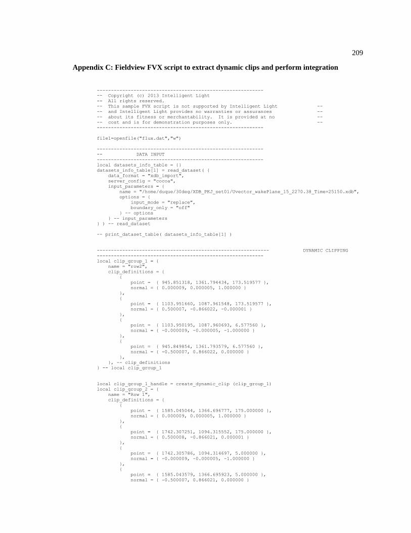
209

Appendix C: Fieldview FVX script to extract dynamic clips and perform integration

-----------------------------------------------------------

-- Copyright (c) 2013 Intelligent Light

-- All rights reserved.

-- This sample FVX script is not supported by Intelligent Light --

-- and Intelligent Light provides no warranties or assurances --

-- about its fitness or merchantability. It is provided at no --

-- cost and is for demonstration purposes only. --

-----------------------------------------------------------

file1=openfile("flux.dat","w")

-----------------------------------------------------------

-- DATA INPUT

-----------------------------------------------------------

local datasets_info_table = {}

datasets_info_table[1] = read_dataset( {

data_format = "xdb_import",

server_config = "cocoa",

input_parameters = {

name = "/home/duque/30deg/XDB_PKJ_set01/Uvector_wakePlane_15_2270.38_Time=25150.xdb",

options = {

input_mode = "replace",

boundary_only = "off"

} -- options

} -- input_parameters

} ) -- read_dataset

-- print_dataset_table( datasets_info_table[1] )

------------------------------------------------------------- DYNAMIC CLIPPING

-----------------------------------------------------------

local clip_group_1 = {

name = "row2",

clip_definitions = {

{

point = { 945.851318, 1361.794434, 173.519577 },

normal = { 0.000009, 0.000005, 1.000000 }

},

{

point = { 1103.951660, 1087.961548, 173.519577 },

normal = { 0.500007, -0.866022, -0.000001 }

},

{

point = { 1103.950195, 1087.960693, 6.577560 },

normal = { -0.000009, -0.000005, -1.000000 }

},

{

point = { 945.849854, 1361.793579, 6.577560 },

normal = { -0.500007, 0.866022, 0.000000 }

},

}, -- clip_definitions

} -- local clip_group_1

local clip_group_1_handle = create_dynamic_clip (clip_group_1)

local clip_group_2 = {

name = "Row 1",

clip_definitions = {

{

point = { 1585.045044, 1366.696777, 175.000000 },

normal = { 0.000009, 0.000005, 1.000000 }

},

{

point = { 1742.307251, 1094.315552, 175.000000 },

normal = { 0.500008, -0.866021, 0.000001 }

},

{

point = { 1742.305786, 1094.314697, 5.000000 },

normal = { -0.000009, -0.000005, -1.000000 }

},

{

point = { 1585.043579, 1366.695923, 5.000000 },

normal = { -0.500007, 0.866021, 0.000000 }

210

},

}, -- clip_definitions

} -- local clip_group_2

local clip_group_2_handle = create_dynamic_clip (clip_group_2)

-----------------------------------------------------------

-- BOUNDARY SURFACES

-----------------------------------------------------------

local boundary_surfs={}

boundary_surfs[1] = create_boundary(

{

transparency = 0,

show_legend = "off",

number_of_contours = 16,

visibility = "on",

line_type = "thin",

geometric_color = 4,

types = {

"Iso Surf 1: CUTTING PLANE = 2270.38 [NORMALS]",

}, -- types

display_type = "mesh_shading",

contours = "none",

vector_func = "none",

scalar_func = "U.vector.x",

dataset = 1,

threshold_func = "none",

show_mesh = "off",

}

) -- boundary_surfs[1]

---

-- Integrate for Ux surface

---

modify (clip_group_1_handle, {

dataset = 1,

active = "on"

})

result = integrate_surface(boundary_surfs[1])

IntUxNx_row2=result.sum_Nx

IntUxNy_row2=result.sum_Ny

IntUxNz_row2=result.sum_Nz


dataset = 1,

active = "on"

})


IntUxNx_row1=result.sum_Nx

IntUxNy_row1=result.sum_Ny

IntUxNz_row1=result.sum_Nz

str=IntUxNx_row1.." "..IntUxNx_row2

---

-- Integrate for Uy surface

---


dataset = 1,

active = "on"

})

modify (boundary_surfs[1], {

scalar_func="U.vector.y"

})


211

IntUyNx_row2=result.sum_Nx

IntUyNy_row2=result.sum_Ny

IntUyNz_row2=result.sum_Nz


dataset = 1,

active = "on"

})


IntUyNx_row1=result.sum_Nx

IntUyNy_row1=result.sum_Ny

IntUyNz_row1=result.sum_Nz

---

-- Integrate for Uz surface

---


dataset = 1,

active = "on"

})

modify (boundary_surfs[1], {

scalar_func="U.vector.z"

})


IntUzNx_row2=result.sum_Nx

IntUzNy_row2=result.sum_Ny

IntUzNz_row2=result.sum_Nz


dataset = 1,

active = "on"

})


IntUzNx_row1=result.sum_Nx

IntUzNy_row1=result.sum_Ny

IntUzNz_row1=result.sum_Nz

--

-- write out results

--

Ux_row1=IntUxNx_row1.." "..IntUxNy_row1.." "..IntUxNz_row1

Uy_row1=IntUyNx_row1.." "..IntUyNy_row1.." "..IntUyNz_row1

Uz_row1=IntUzNx_row1.." "..IntUzNy_row1.." "..IntUzNz_row1

Ux_row2=IntUxNx_row2.." "..IntUxNy_row2.." "..IntUxNz_row2

Uy_row2=IntUyNx_row2.." "..IntUyNy_row2.." "..IntUyNz_row2

Uz_row2=IntUzNx_row2.." "..IntUzNy_row2.." "..IntUzNz_row2

str=Ux_row1.." "..Uy_row1.." "..Uz_row1.." "..Ux_row2.." "..Uy_row2.." "..Uz_row2

write(file1, str, '\n' )

closefile(file1)

212

Appendix D: OpenFOAM code to compute the geometric parameters relevant to ACE

void horizontalAxisWindTurbinesALM_2014_05_01::computeParametersACE()

{

// Zero out the body force to begin with for the current time step...all through the

domain

bodyForce*= 0.0;

scalar thrustSum = 0.0;

scalar torqueSum = 0.0;

scalar thrustBodyForceSum = 0.0;

scalar torqueBodyForceSum = 0.0;

//dimensionedScalar test_pn("pn",dimensionSet(0, 1, 0, 0, 0, 0, 0),10.0);

distNormal*=0; //+= test_pn; //This was just for testing, as time step increases this

becomes a multiple of 10.

distAlongArc*=0; //+=20;//This was just for testing, as time step increases this becomes

a multiple of 20.

fIndexField*=0; //+=30;//This was just for testing, as time step increases this becomes

a multiple of 30.

epsLocal*=0;

etaField*=0; //+=40;//This was just for testing, as time step increases this becomes a

multiple of 40.

cellIndex*=0; //This is not that efficient, but nevertheless works....modify this

later

scalar tolerance = toleranceForACE; // Tolerance for the field searches....better mnake

this input and then copy here

forAll(sphereCells, i)

{

int n = turbineTypeID[i];

//Info<<" Inside the loop for sphereCells"<<endl;

//Info<<"Processor #: "<<Pstream::myProcNo()<<" ...................."<<endl;

Info<<endl<<"Turbine # "<<i<<" Size of Cell Sphere :

"<<sphereCells[i].size()<<endl;

// Proceed to compute ACE parameters for turbine i only if there are sphere cells

on this processor for this turbine.

if (sphereCells[i].size() > 0)

{

forAll(sphereCells[i], m)

{

//Info<<"Sphere Cell #: "<<m<<" ,Cell ID: "<<sphereCells[i][m]<<endl;

if (sphereCells[i][m] == cellIndexToDiagnose)

{

// Create a diagnosis file

diagnosisFile_ = new OFstream("diagnosisFile.txt");

*diagnosisFile_<<"Cell ID: "<<sphereCells[i][m]<<", Cell

Center: ("<<mesh_.C()[sphereCells[i][m]].x()<<", "<<mesh_.C()[sphereCells[i][m]].y()<<",

"<<mesh_.C()[sphereCells[i][m]].z()<<")"<<tab<<"Turbine Type"<<n<<endl;

*diagnosisFile_<<"ActuatorIndex ActPt

ActPtNext vecP vecS ps

pn_orig pn nmin nind dind[]

smin[]"<<endl;

// Create a diagnosis file

//precisionFile = fopen("precisionFile.txt","w");

//fprintf(precisionFile,"abs(pn)-abs(nmin) \t\t +tolerance

\t\t -tolerance\n");

logicFile = fopen("logicFile.txt","w");

}

// For each blade.

forAll(bladeForce[i], j)

{

/* At the current time step, for a particular cell find out

what influence does this

cell have due to blade force ...one blade at a time....so

before visiting each blade reset all the ACE parameters */

int mamax = numBladePoints[i];

//dimensionedScalar

minNormalDist("minNormalDist",dimensionSet(0, 1, 0, 0, 0, 0, 0),1e20);

int nind = 0;

scalar nmin = 0.0;

int dind[101];

scalar smin[101];

213

// For each blade point.

for(int mFort=1; mFort <= mamax-1; mFort++)

{

vector vecP = mesh_.C()[sphereCells[i][m]]

- bladePoints[i][j][mFort-1];

vector vecS = bladePoints[i][j][mFort]

- bladePoints[i][j][mFort-1];

scalar ps = (vecP&vecS)/magSqr(vecS);

vector vec_pn = -ps*vecS + vecP;

scalar pn = mag(vec_pn);

scalar pn_orig = pn;

if ((ps < -tolerance) && (mFort != 1))

pn = mag(vecP);

else if ((ps > (1+tolerance)) && (mFort !=

(mamax-1)))

pn = mag(vecP - vecS);

// Save minimum pn

if (sphereCells[i][m] ==

cellIndexToDiagnose)

{

fprintf(logicFile,"**************** Actuator Index: %d

*****************************\n",mFort);

fprintf(logicFile,"fabs(pn) = %12f

\t, fabs(nmin) = %12f \t, fabs(pn)-fabs(nmin) = %12f \t\t +tolerance = %e \t -tolerance =

%e\n",fabs(pn), fabs(nmin), fabs(pn)-fabs(nmin), tolerance, -tolerance);

}

if ((nind == 0) || ((fabs(pn)-fabs(nmin))

<= tolerance))

{



{

fprintf(logicFile,"Inside

the MAIN 'if' condition\n");

if (nind == 0)

fprintf(logicFile,"\t The condition 'nind == 0' is satisfied\n");

if ((fabs(pn)-fabs(nmin))

<= tolerance)

fprintf(logicFile,"\t The condition '(fabs(pn)-fabs(nmin)) <= tolerance' is satisfied\n");

}

if ((nind == 0) || ((fabs(pn)-

fabs(nmin)) < -tolerance))

{



{

fprintf(logicFile,"\t\t Inside the FIRST 'if' inside MAIN 'if' condition\n");

if (nind == 0)

fprintf(logicFile,"\t\t\t The condition 'nind == 0' is satisfied\n");

if ((fabs(pn)-

fabs(nmin)) < -tolerance)

fprintf(logicFile,"\t\t\t The condition '(fabs(pn)-fabs(nmin)) < -tolerance' is satisfied\n");

}

nind = 1; //

! First minimum OR replacement

dind[nind] = mFort;

nmin = pn;

smin[nind] = ps;

}

else if(nind == 1)

{



{

fprintf(logicFile,"\t\t Inside the FIRST 'else if' inside MAIN 'if' condition\n");

if (nind == 1)


}

214

nind = nind + 1; //

! Allow a second minimum

dind[nind] = mFort;

nmin = pn;

smin[nind] = ps;

}

else if (nind == 2)

{



{

fprintf(logicFile,"\t\t Inside the LAST 'else if' inside MAIN 'if' condition\n");

if (nind == 2)


}

if (mFort != (dind[nind]-

1))

{

if

(sphereCells[i][m] == cellIndexToDiagnose)

{

fprintf(logicFile,"\t\t\t Inside the 'if' condition in the LAST 'else if' inside main 'if'

condition\n");

if

(mFort != (dind[nind]-1))

{

fprintf(logicFile,"\t\t\t\t The condition 'mFort != (dind[nind]-1' is satisfied\n");

fprintf(logicFile,"\t\t\t\t mFort = %d, \t nind = %d, \t dnind[nind] - 1 = %d \n",

mFort,nind,dind[nind]-1 );

}

}

dind[nind] =

mFort; // ! Replace second minimum

nmin = pn;

smin[nind] = ps;

}

}

}


{

*diagnosisFile_<<mFort<<tab;

*diagnosisFile_<<"("<<bladePoints[i][j][mFort-1].x()<<", "<<bladePoints[i][j][mFort-1].y()<<",

"<<bladePoints[i][j][mFort-1].z()<<")"<<tab;

*diagnosisFile_<<"("<<bladePoints[i][j][mFort ].x()<<", "<<bladePoints[i][j][mFort ].y()<<",

"<<bladePoints[i][j][mFort ].z()<<")"<<tab;

*diagnosisFile_<<"("<<vecP.x()<<",

"<<vecP.y()<<", "<<vecP.z()<<")"<<tab;

*diagnosisFile_<<"("<<vecS.x()<<",

"<<vecS.y()<<", "<<vecS.z()<<")"<<tab;

*diagnosisFile_<<tab<<ps<<tab<<pn_orig<<tab<<pn<<tab<<nmin<<tab<<nind<<tab<<tab;

for (int t = 1; t <= nind; t++)

*diagnosisFile_<<dind[t]<<tab;

for (int t = 1; t <= nind; t++)

*diagnosisFile_<<smin[t]<<tab;

*diagnosisFile_<<endl<<endl<<endl;

}

}

// for each actuator point of the i-th turbine and j-th

blade

//Find fIndexField

scalar fIndex = 0.0;

scalar ps;

//scalar ps_sum = 0.0;

for(int t = 1; t <= nind; t++)

{

ps = smin[t];

if (ps < 0) ps = 0;

if (ps > 1) ps = 1;

215

int mFort = dind[t];

fIndex+= 1.0*mFort + ps;

//ps_sum+= ps;


{

//*diagnosisFile_<<"m = "<<mFort<<", ps =

"<<ps<<", ps_sum = "<<ps_sum<<" ,fIndex = "<<fIndex<<endl<<endl;

*diagnosisFile_<<"m = "<<mFort<<", ps =

"<<ps<<" ,fIndex = "<<fIndex<<endl<<endl;

}

}

fIndex = fIndex/(1.0*nind);

//ps = ps_sum/(1.0*nind);


{

*diagnosisFile_<<"For the cell under

diagnosis, pn = "<<nmin<<", ps = "<<ps<<" ,fIndex = "<<fIndex<<endl;

}

// Write the geometric properties to volumeField

distNormal[ sphereCells[i][m]] = nmin;

distAlongArc[sphereCells[i][m]] = ps;

fIndexField[ sphereCells[i][m]] = fIndex;

cellIndex[ sphereCells[i][m]] = sphereCells[i][m];

/* Keep track of cells affected by an actuator point.....

For the i-th turbine, and the m-th cell in its sphere of

influence...

This cell is affected by the actuator index which is same

as "int(fIndex) -1".....

so append this to the list of all the cells affected by

this actuator point */

//int fIndexToTrack = (int)fIndex -1;

//cellsAffected[i][j][fIndexToTrack].append(sphereCells[i][m]);

//psToTrack[i][j][fIndexToTrack].append(ps);

//pnToTrack[i][j][fIndexToTrack].append(pn);

//

***********************************************************************************

// Find etafield

scalar etaFactor = 1.0;

if (fIndex == 1 && ps ==0) //If ps<0 lies to left of first

actuator point

etaFactor = 0.0;

if ((fIndex == mamax) && (ps ==1)) //If ps>0 lies to the

right of last actuator point

etaFactor = 0.0;

int ind = (int)(fIndex);

if (ind < 1)

ind = 1;

if (ind > mamax)

ind = mamax;

int indpo = ind + 1;

if (indpo > mamax)

indpo = mamax;

scalar chordFic_ind = interpolate(bladeRadius[i][j][ind-

1], BladeStation[n], BladeChordFic[n]);

scalar chordFic_indpo =

interpolate(bladeRadius[i][j][indpo-1], BladeStation[n], BladeChordFic[n]);

scalar eps_ind = epsilon[i]*chordFic_ind;

scalar eps_indpo = epsilon[i]*chordFic_indpo;

if (eps_ind < epsilon_min[i])

eps_ind = epsilon_min[i]; // Dimensioned spreading

width

if (eps_indpo < epsilon_min[i])

eps_indpo = epsilon_min[i]; // Dimensioned

spreading width

scalar epsalocal = eps_ind + (fIndex-1.0*ind)*(eps_indpo -

eps_ind);

216

scalar eta = 1.0/(3.1415*epsalocal*epsalocal)*exp(-

pow((nmin/epsalocal),2));

eta = eta*etaFactor;


{

//*diagnosisFile_<<"m = "<<mFort<<", ps =

"<<ps<<", ps_sum = "<<ps_sum<<" ,fIndex = "<<fIndex<<endl<<endl;

*diagnosisFile_<<"ind = "<<ind<<", indpo =

"<<indpo<<", c*(ind) = "<<chordFic_ind<<", c*(indpo) = "<<chordFic_indpo<<", eps(ind) = "<<eps_ind<<",

eps(indpo) = "<<eps_indpo<<", eps_local = "<<epsalocal<<", eta = "<<eta<<endl;

}

// write thelocal epsilon and etaField to volumeField

epsLocal[ sphereCells[i][m]] = epsalocal;

etaField[ sphereCells[i][m]] = eta;

// Now that ACE parameters are computed, compute

"bodyForce"

scalar bf_ind = ind-1;

scalar bf_indpo = indpo-1;

vector incBladeForce = bladeForce[i][j][bf_ind] + (fIndex-

1.0*ind)*(bladeForce[i][j][bf_indpo] - bladeForce[i][j][bf_ind]);// dimension of force

vector incBodyForce = incBladeForce*eta/db[i][bf_ind]; //

bodyForce per unit volume

bodyForce[sphereCells[i][m]] += incBodyForce*factorBodyForce;

thrustBodyForceSum += (-

incBodyForce*mesh_.V()[sphereCells[i][m]]) & uvShaft[i];

torqueBodyForceSum +=

((incBodyForce*mesh_.V()[sphereCells[i][m]])* bladeRadius[i][j][bf_ind] * cos(PreCone[n][j])) &

bladeAlignedVectors[i][j][1];

}// for the j-th blade of the i-th turbine


fclose(logicFile);

} //for each cell for the i-th turbine

}// if sphereCells is not empty

thrustSum += thrust[i];

torqueSum += torqueRotor[i];

}//for each turbine

reduce(thrustBodyForceSum,sumOp<scalar>());

reduce(torqueBodyForceSum,sumOp<scalar>());

// Print information comparing the actual thrust and torque to the integrated body

force.

Info << "Thrust from Body Force = " << thrustBodyForceSum << tab << "Thrust from Act.

Line = " << thrustSum << tab << "Ratio = " << thrustBodyForceSum/thrustSum << endl;

//Info << "Torque from Body Force = " << torqueBodyForceSum << tab << "Torque from Act.

Line = " << torqueSum << tab << "Ratio = " << torqueBodyForceSum/torqueSum << endl;

}//function

VITA

Pankaj Kumar Jha

Pankaj Kumar Jha was born and raised in India, in the states of Bihar and Jhakhand. His early

upbringing amongst carpenters, blacksmiths, and astrologers and later at an industrial township, involving

works in mining, metallurgical, and mechanical engineering nurtured his engineering mindset and

triggered his curiosity about earth and space science. It was during high school (tenth grade) that he

decided to learn and contribute to the science and art of flight. He earned an Integrated M.Sc. in

Mathematics and Computing along with a minor in Aerospace Engineering at Indian Institute of

Technology (IIT), Kharagpur. He worked on turbomachinery aerodynamics and database programming at

GE Aviation in Bangalore before joining Penn State. Apart from the work presented in this dissertation,

he has worked on some other projects at Penn State. These include the work on ducted fans, helicopter

rotor hub, and airfoil and wind turbine icing.

Documents

CHARACTERIZATION OF WAKE TURBULENCE IN A WIND TURBINE