Embed Size (px)
Citation preview

Characterization of the Stiffness of Unbound Materials forPavement Design: Do We Follow the Right Approach?
Angel Mateos, Ph.D.1; and Jorge B. Soares, Ph.D.2
Abstract: Two main approaches have been followed to determine the modulus of unbound materials in six asphalt pavement sections testedat the CEDEX test track. The first one consists on back-calculation from the deflection bowls measured under the load of a falling weightdeflectometer. In the second approach, a nonlinear constitutive relationship is calibrated from repeated load triaxial testing, and layer modulusis estimated through this relationship for the stresses calculated under traffic loads by using a multilayer linear elastic model. Significantdifferences were found between the two procedures, with back-calculation resulting in higher modulus. The two approaches were evaluatedby comparing model predictions to actual response measured under the load of the traffic simulation vehicles of the test track. The resultsindicate that back-calculation provided more realistic estimations of the stiffness of unbound materials than the laboratory approach. This lastapproach significantly underestimated the stiffness of granular materials located at shallow depths in the pavement structure. DOI: 10.1061/(ASCE)TE.1943-5436.0000645. © 2014 American Society of Civil Engineers.
Author keywords: Mechanistic-empirical design; Pavement instrumentation; Unbound materials characterization.
Introduction
Mechanistic-empirical design methods are increasingly gainingacceptance in the pavement community, and they have beenadopted as the official design procedure by many road authoritiesworldwide (Soares et al. 2009). These methods conceive pave-ments as multilayered structures subjected to environment andtraffic loads: stresses and strains at critical locations are usedto predict distress levels by using simplified damage models–commonly fatigue laws–which still incorporate a high degreeof empiricism.
Different mechanistic models have been used to determine pave-ment structural response to traffic vehicles, with the multilayerlinear elastic (m.l.e.) solution under static load (Burmister solution)the most widely used. Either by an apparent Young moduluswhen using m.l.e. models, or by a more advanced constitutive re-lationship when using finite-element programs, soils and granularmaterials layers have to be characterized in a realistic way. Thischaracterization represents the main issue of any pavement designmethodology, and it has been typically dealt with by adopting oneof the three following alternatives:1. Laboratory or field testing of the actual materials (both will be
investigated in this paper).2. Estimating modulus from other material parameters, like plas-
ticity index, CBR (California bearing ratio), and gradation.3. Adopting representative values as a function of soil or granular
material type.
These three alternatives constitute the hierarchical approachadopted by the current AASHTO pavement design procedure(AASHTO 2008), widely known as the MEPDG (mechanistic-empirical pavement design guide). The highest reliability isachieved with the first alternative, by testing actual materialseither in the laboratory or in the field. In the first case, repeatedload triaxial testing is conducted by applying different stressconditions–confining and deviator stresses–and measuring axialand, depending on the standard, radial deformation. Stiffness isestimated for each cycle by using the strain recovered after peakload, which results in an effective modulus termed resilientmodulus. In the case of field testing, the generalized procedureis the back-calculation of stiffness parameters–typically Youngmodulus–from deflection bowls measured under the load of aFWD (falling weight deflectometer). This device applies a pulseload whose length, typically 20–60 ms, is representative of amoving vehicle. Even though both options–laboratory and fieldtesting–have been widely recommended and recognized, it is alsoaccepted that they result in quite different stiffness estimations.Discrepancies between both procedures have been reported in theopen literature, with the FWD back-calculated moduli being typ-ically higher than the laboratory measured moduli for equivalentstress state: Nazarian et al. (1998) obtained ratios FWD/lab in theinterval 1.4–1.9 for granular bases; Ping et al. (2002) obtained aratio of 1.65 for granular subgrades; Rahim and George (2003)reported ratios between 0.85 and 2.0 for clayey and sandy sub-grade soils, and Ji et al. (2012) obtained ratios between 1.6 and5.0 for subgrade soils. Several reasons have been provided forsuch discrepancies, like differences between laboratory and fieldcompaction, long-term effects on the in situ materials (such asdegradation or cementation of particles), differences betweenFWD and triaxial test pulse loads, and the inability of the labo-ratory tests to simulate the actual confinement and the effect ofthe surrounding material on the in situ material’s response (VonQuintus and Killingsworth 1998). These studies show the highvariability and low correlation between FWD and lab results,which reflects that a simple relationship between both ap-proaches probably does not exist.
1Civil Engineering, CEDEX Transport Research Center, Autovía deColmenar Viejo km 18, Madrid 28760, Spain (corresponding author).E-mail: [email protected]
2Civil Engineering, Universidade Federal do Ceará—Laboratório deMecânica dos Pavimentos, Campus do Pici S/N, Bloco 703, 60455-760Fortaleza, Ceará, Brazil. E-mail: [email protected]
Note. This manuscript was submitted on May 21, 2013; approved onNovember 7, 2013; published online on January 6, 2014. Discussion periodopen until June 6, 2014; separate discussions must be submitted for indi-vidual papers. This paper is part of the Journal of Transportation Engi-neering, © ASCE, ISSN 0733-947X/04014001(9)/$25.00.
© ASCE 04014001-1 J. Transp. Eng.
J. Transp. Eng. 2014.140.
Dow
nloa
ded
from
asc
elib
rary
.org
by
HU
NT
LIB
RA
RY
AC
Q D
EPT
on
10/2
7/14
. Cop
yrig
ht A
SCE
. For
per
sona
l use
onl
y; a
ll ri
ghts
res
erve
d.

Problem Statement
It is highly remarkable that despite numerous studies comparingFWD versus lab moduli exist, little effort has been dedicated todetermine which of the two approaches better represents pavementstructural behavior under traffic loads. When the unbounded ma-terial’s modulus was treated as an input variable for the statisticalcalibration of pavement design procedures (as was the case for“Resilient Modulus of Roadbed Soil” in the 1993 AASHTO designguide), there was not an immediate need to answer that question.However, when mechanistic-empirical design methods are fol-lowed, and the unbounded material’s modulus is used within amultilayered model to predict pavement response to traffic loads,the need to answer the question is evident. At present, the mostcommon approach is the use of the laboratory modulus determinedfor a stress state representative of in situ stress conditions undertraffic loads. This is the approach adopted by the MEPDG, which
establishes the need to apply adjustment factors when moduli ofsoils and granular layers are obtained from FWD back-calculation.It is worth noting that no matter which adjustment factors are usedfor correcting the unbound layer’s moduli, the use of any factorother than 1 implies that our structural response model will notbe able to predict pavement response under the load of a FWD,which is supposedly designed to resemble traffic loads.
Objective
The objective of the research here presented is the comparisonof two approaches to determine the modulus of unbound materi-als, FWD back-calculation and laboratory repeated load triaxialtesting, and the evaluation of the two approaches in terms oftheir ability to predict pavement structural response under trafficloads.
Research Approach
Experimental data for this research come from six asphalt pavementsections tested at the CEDEX full-scale test track (Fig. 1). This fa-cility consists of a closed circuit with a total travel distance of300 m and two automatic vehicles simulating real traffic. Pavementsections are built along the 75-m-long tangents of the track, inside areinforced concrete test pit (2 m deep and 8 m wide), by using con-ventional road-building procedures. The pavement structuresconsisted of a 120–150-mm asphalt layer placed directly on topof the subgrades (Fig. 2). A 150-mm asphalt layer was used forsection 1 on top of the reference subgrade, and 120 mm was usedfor sections 2–6 on an improved subgrade. The improvement wasachieved by either introducing cement-stabilized soils in thecapping layer or by introducing medium to high quality soils be-tween the soil 3 capping layer and the soil 0 embankment. Labo-ratory characterization of the different soils is presented in Table 1.The test lasted two and a half years, during which the automaticvehicles applied 1,323,600 load repetitions of a 6.5-ton half-axlewith dual tires [800 kPa (8-bar inflation pressure)].
Fig. 1. CEDEX test track
Fig. 2. Sections layout and instrumentation
© ASCE 04014001-2 J. Transp. Eng.
J. Transp. Eng. 2014.140.
Dow
nloa
ded
from
asc
elib
rary
.org
by
HU
NT
LIB
RA
RY
AC
Q D
EPT
on
10/2
7/14
. Cop
yrig
ht A
SCE
. For
per
sona
l use
onl
y; a
ll ri
ghts
res
erve
d.

Sections were instrumented in order to measure the structuralresponse under the 6.5-ton (half-axle) traffic simulation vehicles(Fig. 2). Sensor records were automatically registered throughoutthe test and analyzed with specially dedicated software. Eachrecord consists of the sensor response as vehicle approaches(−5 m) and leaves (þ5 m) sensor longitudinal position. The10-m-long records were automatically registered at regular cycleintervals, and stored together with cycle number and vehicle andenvironment data (vehicle number, speed and transverse position,and air and asphalt temperature). The specially dedicated softwareautomatically analyzes the records and extracts the peak values thathave been used for model validation in this study. Additionalinformation on this process can be found in Pérez Ayuso et al.(2008). All sensor data presented in this paper were collected withvehicles moving at 20–30 km=h and for the transverse position cor-responding to sensors right below the center of the dual wheel.Only data registered at the beginning of the test, before cycle70,000, were used for this particular research, since the first signifi-cant rainfall took place around cycle 72,000. Moisture condition ofunbound materials along this initial period can be assumed to beclose to the modified Proctor optimum moisture content that wastargeted during construction. The same moisture content wasadopted for laboratory triaxial specimens, so that both sourcesof information–lab and field–could be directly compared.
FWD testing was conducted after construction of the sections,and soils moduli were determined through back-calculation by us-ing Evercalc 5.20. This program incorporates an m.l.e. model thatis run iteratively by changing moduli of the different layers until asatisfactory match is found between calculated and measured de-flection bowls. Evercalc is a linear model, which means that result-ing moduli will only be applicable when the pavement structure issubjected to load levels that are similar to those applied by theFWD. For this reason, the FWD load used for back-calculationwas 6.5 tons, weight of the traffic simulation vehicles, so that re-sulting moduli could be used to predict pavement structural re-sponse under the pass of such vehicles. Loading plate diameterwas 300 mm. Evercalc is also a static model, which means thatresulting moduli will be representative of the mean frequency ofthe FWD load pulse, which was 15 Hz in this particular study. Thiswill have a limited effect on some plastic soils whose modulus mayexhibit some time-dependency. One layer was assumed in the modelfor each actual pavement layer, which means that the stiffness gra-dient of the different layers could not be determined: each value re-sulting from back-calculation can be regarded as an overall mean ofthe corresponding layer. For sections 2 and 3, additionally, soil 1 and
soil 0 courses were merged into one due to the uncertainties of back-calculation technique for detecting the modulus of a small-thicknesslayer under relatively rigid materials like cement-stabilized soil. Thisstabilized material presented a compressive strength of 2.3 MPa afterseven days, and a modulus of 1,500 MPa was determined throughback-calculation at the beginning of the test.
Repeated load triaxial testing was conducted for soils 0 through3 following AASHTO T307-99 (AASHTO 2007), and a slightlymodified version of Uzan universal model (Uzan 1985), accordingto Eq. (1), was calibrated. This formulation is virtually the sameas the one used in the MEPDG, but including the deviator term,q, instead of the octahedral shear stress, τoct. Once the model iscalibrated from laboratory data, it is applied to the field three-dimensional (3D) stress state by substituting q with 3 · τoct=ð21=2Þ.This way, Eq. (1) produces the same results as the MEPDG formu-lation. Proctor modified maximum density, ϒmax, and optimummoisture content, ωopt:, were targeted for preparing the laboratoryspecimens. In situ density was around 98% of ϒmax for the im-proved subgrade and around 95% ϒmax for soil 0 embankment.No triaxial testing was conducted for the cement-stabilized soil,since laboratory testing showed that the mechanical behavior of thismaterial was essentially linear for the stress levels considered inthis study.
MR ¼ k0
�pσref
�k1�
qσref
þ 1
�k2 ð1Þ
where MR = resilient modulus; p = mean normal stress,ðσ1 þ σ2 þ σ3Þ=3; q = deviator stress, σ1-σ3; σref ¼ 0.1 MPa(reference stress); and k0, k1, k2 are model parameters.
Results and Discussion
Comparison of FWD Back-Calculated Modulus versusLaboratory Results
The pseudo-nonlinear approach of Kenlayer (Huang 1993) wasused to determine the elastic modulus of each layer when unboundmaterials were characterized by the laboratory-calibrated nonlinearconstitutive relationship of Eq. (1). According to this approach,each layer is divided in a number of sublayers whose moduliare determined in an iterative process as a function of stress com-puted by an m.l.e. program at a certain characteristic point in eachsublayer. Horizontal variation of modulus is not considered in thisapproach, and neither a failure criteria. The total maximum numberof sublayers for each pavement section was 10, since this was thelimitation of the Bisar (De Jong et al. 1979) m.l.e. program used forthe present research. Soil and asphalt layer weight, as well as lateralearth stress, are added to m.l.e. model stresses in order to computeresilient modulus according to Eq. (1). The iterative process con-tinues until modulus convergence is achieved. A similar approachis proposed by Von Quintus and Killingsworth (1997) and is rec-ommended in the MEPDG. The modulus obtained for each layer, asa weighted mean value of the different sublayers, is referred to asthe laboratory apparent modulus of the layer hereafter.
A constitutive law, according to Eq. (1), was calibrated for eachsoil based on laboratory triaxial data, resulting in the model param-eters presented in Table 2. Soil 0 presents a high (in absolute value)k2 exponent and a low k1, which is typical of a cohesive materialwhose stiffness decreases as shear stresses (distortion) increase.Soils 2 and 3 present the typical behavior of a granular material,whose modulus increases as confinement increases (high k1 expo-nent). Soil 1 behavior is between cohesive and granular, but closerto the former.
Table 1. Soils Characterization in the Laboratory
Test result Soil 0 Soil 1 Soil 2 Soil 3
Percent passing# 20 mm 85.9 97.7 82.2 100# 2 mm 65.8 86.1 35.9 50.7# 0.4 mm 57.7 48.3 17.0 31.2# 0.08 mm(no. 200)
46.3 31.5 5.9 16.5
Liquid limit 37.6 34.8 nonplastic nonplasticPlasticity index 19.3 18.0
Modified Proctorϒmax 1.88 2.07 2.19 2.20ωopt 12.2 7.9 5.7 5.8
Soaked CBR95% ϒmax 4.5 9.6 33.5 66.2100% ϒmax 5.9 27.4 83.3 136.7
© ASCE 04014001-3 J. Transp. Eng.
J. Transp. Eng. 2014.140.
Dow
nloa
ded
from
asc
elib
rary
.org
by
HU
NT
LIB
RA
RY
AC
Q D
EPT
on
10/2
7/14
. Cop
yrig
ht A
SCE
. For
per
sona
l use
onl
y; a
ll ri
ghts
res
erve
d.

The modulus of the asphalt layer had to be assumed in the iter-ative process. This value was determined in the laboratory, byconducting temperature and frequency sweep dynamic modulustesting in compression. A frequency of 15 Hz was selected asrepresentative of the load pulse of the KUAB FWD device withthe particular weight-buffer configuration adopted in this study.The validity of asphalt layer modulus determined in the laboratoryis supported by the excellent agreement that was found with FWDback-calculation results (Mateos et al. 2012a). Asphalt layer tem-perature (mean value from two thermocouples) varied between 20and 49°C during FWD measurements, with a mean value of 32°C.This temperature was then selected to determine the modulus. Themodulus of the cement-stabilized layer was also fixed in the iter-ative process: 1,500 MPa, as resulting from FWD back-calculation.
The laboratory apparent modulus of the different layers (ELab)are compared to FWD back-calculated values (EFWD) in Fig. 3.Two points are included for each layer and section, correspondingto two different offsets: the center of the wheel path and a parallelline 2.5 m apart. Each FWD back-calculated value represents theaverage of three measurements where 16–20 longitudinal pointsper section were tested. A reasonable agreement was obtained be-tween measured and theoretical deflection bowls: the root-mean-square error presented an average value of 2.9% through all inversecalculations, and it was below 4% in 80% of the cases. The resultspresented in Fig. 3 agree with previous studies that show thatmodulus predictions based on laboratory data are lower thanFWD back-calculation results. The average ratios EFWD=ELab were2.7 for soil 3 capping layer, 2.2 for the intermediate layer ofsections 4–6, 1.4 for soils below the cement-stabilized layer ofsections 2–3, and 1.3 for the soil 0 embankment. Except for soil0, these values are not very different from MEPDG recommendedadjustment factors that are 1.9 for soils below an asphalt pavementwithout a granular base (sections 1, 4, 5, and 6) and 1.3 for soilsbelow a stabilized subgrade (sections 2 and 3). The results are alsoin line with other studies that show that a better agreement is ob-tained for unbound materials that are deeper in the pavementstructure (Parker and Elton 1990; Seeds et al. 2000). A reasonablecorrelation (compared to similar studies) was found between lab
and field results (R2 ¼ 0.58), although it is not likely that acalibrated empirical relationship could be extrapolated to otherpavement sections and materials. In general, the laboratory appar-ent modulus of the layers did not significantly change from onesection to another, and even changes between different materialswere very reduced, as reflected in Fig. 3. The opposite happenedfor FWD back-calculated moduli, which varied considerably be-tween materials and sections.
Comparison of Model Prediction versus MeasuredStructural Response
Structural response was estimated under the traffic simulationvehicles by using the Bisar m.l.e. model. Two approaches for thedetermination of soils moduli were followed: FWD back-calculationand laboratory triaxial testing. In the first case, back-calculatedmoduli were direct inputs to the model, while in the second case,the Kenlayer pseudo-nonlinear approach was followed. Asphaltlayer modulus was determined from laboratory data (dynamicmodulus testing in compression) as a function of temperature, ve-hicle speed (20–30 km=h for this comparison) and layer thickness.Further details on asphalt characterization can be found in Mateoset al. (2012b).
Measured and predicted responses are presented in Figs. 4–7 interms of surface deflection, longitudinal strain at the bottom of theasphalt layer and vertical stress at the top of soil 3 capping layer andsoil 0 embankment. As a general rule, two sensors per section wereavailable for each variable. Three sensors per section were used forasphalt longitudinal strain in sections 2 and 3, since previous ex-periences had shown a high variability when strain was measuredbetween asphalt and a cement treated layer. Only one pressure cellper section was used at the top of soil 0 in sections 4–6, since a verylow stress level was anticipated. It should be noted that three sen-sors did not work properly and were not included in this study (anasphalt strain gage in section 5, a stress cell in section 6 soil 3 andanother one in section 1 soil 0). No information is included forsection 4 due to a problem with its data acquisition system atthe beginning of the test.
It is important to bear in mind that the process of measuring thestructural response of pavements is not as reliable as in other civilengineering structures, as can be deduced from the relatively highwithin and between sensor variability in Figs. 4–7. Most differen-ces between sections could be attributed to actual differences in thestructure of the sections, but construction variability and measure-ment variability played also an important role.
The first conclusion that can be extracted from Figs. 4–7 is thatthe m.l.e. model, calibrated from FWD back-calculation, providesan overall good prediction of the stress-strain state developed in aflexible pavement structure under a moving wheel. Prediction er-rors are within sensor to sensor variability range for most variables.A slight underestimation of deflections seems to happen, whichdoes not seem to be related to the asphalt or capping layer modulus,since asphalt strain and vertical stress at the top of subgrades areadequately predicted. Consequently, it is likely related to an over-estimation of soil 0 embankment modulus. This could be attributedto a slight time-dependency of the modulus of this plastic soil, to-gether with the fact that the representative frequency of the movingvehicle, below 2.5 Hz, was much smaller than the representativefrequency of the FWD pulse, which was 15 Hz. The FWD-calibrated model underpredicted vertical stress at the top of the sub-grade of section 5 and at the top of soil 0 in section 3. No definitiveexplanation was found for this underestimation, which happenedmore sharply for the lab-calibrated models. On the contrary, themodel overestimated vertical stress at the top of soil 0 in section 6,Fig. 3. Comparison of FWD back-calculation versus laboratory results
Table 2. Parameters of Soils’ Constitutive Equation [Eq. (1)]
Material k0 (MPa) k1 k2
Soil 0 123 0.296 −0.929Soil 1 155 0.375 −0.754Soil 2 159 0.615 −0.200Soil 3 173 0.743 −0.092
© ASCE 04014001-4 J. Transp. Eng.
J. Transp. Eng. 2014.140.
Dow
nloa
ded
from
asc
elib
rary
.org
by
HU
NT
LIB
RA
RY
AC
Q D
EPT
on
10/2
7/14
. Cop
yrig
ht A
SCE
. For
per
sona
l use
onl
y; a
ll ri
ghts
res
erve
d.
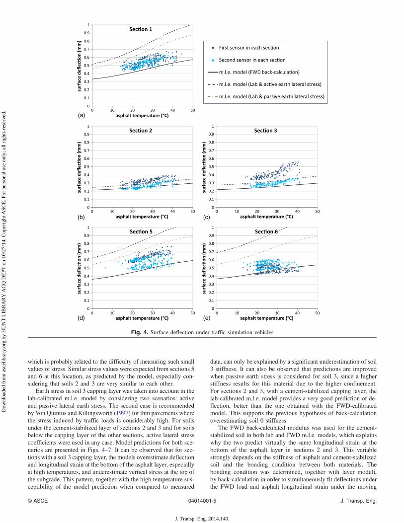
which is probably related to the difficulty of measuring such smallvalues of stress. Similar stress values were expected from sections 5and 6 at this location, as predicted by the model, especially con-sidering that soils 2 and 3 are very similar to each other.
Earth stress in soil 3 capping layer was taken into account in thelab-calibrated m.l.e. model by considering two scenarios: activeand passive lateral earth stress. The second case is recommendedby Von Quintus and Killingsworth (1997) for thin pavements wherethe stress induced by traffic loads is considerably high. For soilsunder the cement-stabilized layer of sections 2 and 3 and for soilsbelow the capping layer of the other sections, active lateral stresscoefficients were used in any case. Model predictions for both sce-narios are presented in Figs. 4–7. It can be observed that for sec-tions with a soil 3 capping layer, the models overestimate deflectionand longitudinal strain at the bottom of the asphalt layer, especiallyat high temperatures, and underestimate vertical stress at the top ofthe subgrade. This pattern, together with the high temperature sus-ceptibility of the model prediction when compared to measured
data, can only be explained by a significant underestimation of soil3 stiffness. It can also be observed that predictions are improvedwhen passive earth stress is considered for soil 3, since a higherstiffness results for this material due to the higher confinement.For sections 2 and 3, with a cement-stabilized capping layer, thelab-calibrated m.l.e. model provides a very good prediction of de-flection, better than the one obtained with the FWD-calibratedmodel. This supports the previous hypothesis of back-calculationoverestimating soil 0 stiffness.
The FWD back-calculated modulus was used for the cement-stabilized soil in both lab and FWD m.l.e. models, which explainswhy the two predict virtually the same longitudinal strain at thebottom of the asphalt layer in sections 2 and 3. This variablestrongly depends on the stiffness of asphalt and cement-stabilizedsoil and the bonding condition between both materials. Thebonding condition was determined, together with layer moduli,by back-calculation in order to simultaneously fit deflections underthe FWD load and asphalt longitudinal strain under the moving
(a)
(b) (c)
(d) (e)
Fig. 4. Surface deflection under traffic simulation vehicles
© ASCE 04014001-5 J. Transp. Eng.
J. Transp. Eng. 2014.140.
Dow
nloa
ded
from
asc
elib
rary
.org
by
HU
NT
LIB
RA
RY
AC
Q D
EPT
on
10/2
7/14
. Cop
yrig
ht A
SCE
. For
per
sona
l use
onl
y; a
ll ri
ghts
res
erve
d.

vehicles. This explains the good agreement that was achieved forthis last variable. A specially dedicated software was programmedfor conducting this back-calculation.
Discussion
The lack of agreement obtained between laboratory moduli andFWD back-calculation results is not surprising, as it has been pre-viously shown by many studies. The comparison of m.l.e. modelpredictions to actual measured response indicates that an overallgood agreement is achieved when moduli of the unbound layersare determined from FWD back-calculation. On the contrary, whenlab-calibrated constitutive relationships are used for soil characteri-zation, the m.l.e. model fails to predict measured response. Thisfailure is mainly related to the underestimation of the stiffnessof soil 3 capping layer, whose modulus is 2 to 3 times what wouldbe expected from laboratory triaxial testing. Such underestimation
is not related to actual density of the material, since in situ densitywas approximately 2% lower than that achieved in triaxialspecimens, and it is neither related to moisture changes betweenconstruction and FWD testing, as indicated by time-domain reflec-tometry sensors located in this material.
Soil 3 come from a tunnel boring machine excavation in gran-ite rocks, and its gradation is not very different from the typicalgranular bases used in flexible pavements. The granular nature ofthis material was previously shown in terms of k-parameters re-flected in Table 2. As a consequence, the subgrade capping layercan be also regarded as a granular base plus a granular subbase.With this consideration, the 2.7 ratio EFWD=ELab that was ob-tained for the capping layer is almost identical to values reportedby Parker and Elton (1990), who obtained a mean ratio of 2.8 forgranular bases and subbases, and Seeds et al. (2000), who ob-tained ratios between 2 and 3 for granular bases. An attemptto explain these results has to consider the differences betweenthe mechanistic behavior of a granular material and the linear
(a)
(b) (c)
(d) (e)
Fig. 5. Asphalt longitudinal strain under traffic simulation vehicles
© ASCE 04014001-6 J. Transp. Eng.
J. Transp. Eng. 2014.140.
Dow
nloa
ded
from
asc
elib
rary
.org
by
HU
NT
LIB
RA
RY
AC
Q D
EPT
on
10/2
7/14
. Cop
yrig
ht A
SCE
. For
per
sona
l use
onl
y; a
ll ri
ghts
res
erve
d.

elastic material model assumed to determine the laboratory ap-parent modulus of the layer.
Mechanical behavior of a granular material is determined byits particulate nature, which confers strong nonlinearity on thismaterial and determines its response to imposed actions. Insteadof a continuum medium, an aggregate skeleton is formed by par-ticles packed closely together. Aggregate interlock increases forincreasing confining pressure, which explains the influence ofthis variable on the modulus. Only a very minor part of the macro-scopic deformation of these materials under load is due to defor-mation of the particles; almost all of it is due to particles slidingor rolling on other particles. Besides, shear strains force particlesto climb on each other, which tends to increase the bulk volumeof the material. This explains shear dilatancy and shear softeningas well as the high Poisson ratios—even higher than 1—thathave been reported from laboratory triaxial testing (Uzan 1992).This type of performance has been successfully explained byUllidtz (1997), using the discrete element method (DEM). Ullidtzshows that while a reasonable prediction of vertical stresses in aparticulate media can be achieved by using linear elasticity, thesame is not applicable to horizontal stresses. In general, horizontalstress predicted by DEM is much higher than predicted by lin-ear elastic theory, which frequently results in negative (tension)values. The same outcomes were obtained by Hoff et al. (1999)based on hyperelasticity theory, which can be used to model sheardilatancy. According to these results, the m.l.e. model will under-predict material confinement in the field. Consequently, an under-estimation of the stiffness can be expected when predicted meanstress is input to the laboratory-calibrated nonlinear constitutiverelationship of a typical granular material. This underestimationwill be more significant as shear stresses become importantcompared to confining stress, e.g., for granular materials under
small-thickness asphalt layers like the soil 3 capping layer in thisexperiment.
A better agreement (EFWD=ELab ¼ 1.3) was achieved for soil 0embankment. The stiffness of this material is mainly determinedby the amount of shear distortion, quantified by the deviator stressin triaxial testing or by the octahedral shear stress in the field.The particulate nature of this soil is much less pronounced thanin soil 3, which makes the linear elastic theory (based on continu-ity) more applicable. The same can be said of the combination ofsoil 1 intermediate layer and soil 0 embankment in sections 2 and 3,where a ratio EFWD=ELab of 1.4 was obtained. Stresses are rela-tively low in both situations, as well as distortion compared to con-finement. This might be another reason for the better agreementbetween Lab moduli and FWD back-calculation, which is in linewith other studies reporting the same result for unbound materialsthat are deeper in the pavement structure (Parker and Elton 1990;Seeds et al. 2000).
These results question the adoption of the laboratory approachas the reference or true approach for mechanistic-empirical pave-ment design. If this approach was followed for the sections withsoil 3 capping layer of this study, a significant overestimation ofthe longitudinal strain at the bottom of the asphalt layer and thevertical strain at the top of the subgrade would result. Thesetwo variables are of main importance for predicting the evolutionof structural distresses and, consequently, pavement life. The lim-itations of this approach are not related to the laboratory testing,but to the m.l.e. model that is used to calculate stresses. A majorimprovement would be expected if a realistic material model wereimplemented in the calculations, by using the discrete-elementmethod, nonlinear hyperelasticity, or a stress-dependent model withfailure criteria.
(a)
(b) (c)
Fig. 6. Vertical stress at the top of the subgrade (soil 3) under traffic simulation vehicles
© ASCE 04014001-7 J. Transp. Eng.
J. Transp. Eng. 2014.140.
Dow
nloa
ded
from
asc
elib
rary
.org
by
HU
NT
LIB
RA
RY
AC
Q D
EPT
on
10/2
7/14
. Cop
yrig
ht A
SCE
. For
per
sona
l use
onl
y; a
ll ri
ghts
res
erve
d.

Conclusions
Two different approaches have been followed to determine themoduli of unbound materials layers: FWD back-calculation andlaboratory repeated load triaxial testing. The moduli of the layersthat were obtained by the laboratory approach did not significantlychange from one section to another, and even changes between dif-ferent materials were very reduced. The opposite happened forFWD back-calculated moduli, which considerably varied betweenmaterials and sections. A ratio EFWD=ELab of 2.7 was obtained for ahigh-quality granular soil located under a 120–150-mm asphaltlayer. A better agreement, ratios EFWD=ELab of 1.3–1.4, was ob-tained for cohesive soils located deeper in the pavement sections.The two approaches have been evaluated in terms of their ability topredict the structural response that was measured in full-scale sec-tions tested at the CEDEX test track. Different conclusions can beextracted from this evaluation.• FWD back-calculation provided realistic values for the modulus
of soils and granular materials layers, which were used in a
multilayer linear elastic model to predict key variables ofpavement response that are typically used within the frameof mechanistic-empirical design.
• The laboratory approach significantly underestimated the mod-ulus of the high-quality granular soil located at the top of thesubgrades, but provided realistic values for the modulus of co-hesive soils located deeper in the pavement structure or sub-jected to low shear stresses.
• When the stresses predicted by a multilayer linear elastic modelare used to compute the modulus of a granular layer, by meansof a laboratory-calibrated nonlinear constitutive relationship, anunderestimation of the stiffness can be expected. This underes-timation will be more significant as shear stresses become im-portant compared to confining stress, e.g., for granular materialsunder small-thickness asphalt layers.
• The adoption of the laboratory approach as the reference or trueapproach for any situation, which is a common option inmechanistic-empirical design, is questioned by the experimentalresults obtained in the present research. The application of an
(a)
(b) (c)
(d) (e)
Fig. 7. Vertical stress at the top of soil 0 embankment under traffic simulation vehicles
© ASCE 04014001-8 J. Transp. Eng.
J. Transp. Eng. 2014.140.
Dow
nloa
ded
from
asc
elib
rary
.org
by
HU
NT
LIB
RA
RY
AC
Q D
EPT
on
10/2
7/14
. Cop
yrig
ht A
SCE
. For
per
sona
l use
onl
y; a
ll ri
ghts
res
erve
d.
adjustment factor to FWD back-calculation results is alsoquestioned. It is expected, though, that both approaches willproduce similar results as soon as realistic models are usedfor granular materials, that adequately take into account theirparticulate nature.
Acknowledgments
Results presented here come from a full-scale experiment that wasfunded by the Spanish General Road Directorate. The authors ofthis paper would like to express their gratitude to this institution.
References
AASHTO. (2007). “Standard method of test for determining the resilientmodulus of soils and aggregate materials.” T 307-99, Washington, DC.
AASHTO. (2008). “Mechanistic-empirical pavement design guide, interimedition: A manual of practice.” Washington, DC.
De Jong, L., Peutz, M. G. F., and Korswagen, A. R. (1979). Computer pro-gram BISAR, layered systems under normal and tangential surfaceloads, Koninklijke/Shell-Laboratorium, Amsterdam, Netherlands.
Evercalc 5.20 [Computer software]. Washington State Dept. of Transpor-tation Materials Laboratory, Olympia, WA.
Hoff, I., Nordal, S., and Nordal, R. S. (1999). “Constitutive model for un-bound granular materials based on hyperelasticity.” Unbound granularmaterials—laboratory testing, in-situ testing and modelling, A. GomesCorreia, ed., A. A. Balkema, Rotterdam, Netherlands, 187–196.
Huang, H. (1993). Pavement analysis and design, Prentice Hall,Englewood Cliffs, NJ.
Ji, Y., Siddiki, N., Nantung, T., and Kim, D. (2012). “Effect of moisturevariation on subgrade and base material MR design values and its im-plementation in MEPDG.” Proc., Transportation Research Board 91stAnnual Meeting, Transportation Research Board, Washington, DC.
Mateos, A., Ayuso, J., Cadavid, B., and Marrón, J. (2012a). “Lessonslearned from the application of CalME asphalt fatigue model to exper-imental data from CEDEX test track.” Advances in Pavement Designthrough Full-scale Accelerated Pavement Testing, Taylor & FrancisGroup, London.
Mateos, A., Ayuso, J., and Cadavid, B. (2012b). “Evolution of asphaltmixture stiffness under the combined effects of damage, aging and
densification under traffic.” Transport Research Record 2304, Trans-portation Research Board, Washington, DC, 185–194.
Nazarian, S., Rojas, J., Pezo, R., Yuan, D., Abdallah, I., and Scullion, T.(1998). “Relating laboratory and field moduli of Texas base materials.”Transportation Research Record, Transportation Research Board,Washington, DC, 1–11.
Parker, F., and Elton, D. J. (1990). Methods for evaluating resilient moduliof paving materials, Auburn Univ. Highway Research Center, Auburn,AL.
Pérez Ayuso, J., Cadavid, B., and Mateos, A. (2008). “Managing data frominstrumentation in the CEDEX test track.” Proc., 3rd Int. Conf. onAccelerated Pavement Testing, Transportation Research Board, Madrid.
Ping, W. V., Yang, Z., and Gao, Z. (2002). “Field and laboratory determi-nation of granular subgrade moduli.” J. Perform. Constr. Facil., 10.1061/(ASCE)0887-3828(2002)16:4(149), 149–159.
Rahim, A. A., and George, K. P. (2003). “Falling weight deflectometer forestimating subgrade elastic moduli.” J. Transp. Eng., 10.1061/(ASCE)0733-947X(2003)129:1(100), 100–107.
Seeds, S. B., Alavi, S. H., Ott, W. C., Mikhail, M., and Mactutis, J. A.(2000). “Evaluation of laboratory determined and nondestructivetest based resilient modulus values from the westrack experiment.”Nondestructive testing and backcalculation of moduli, ASTM, WestConshohocken, PA.
Soares, J. B., Mateos, A., and Goretti da Motta, L. M. (2009). “Aspectosgerais de métodos de dimensionamento de pavimentos asfálticos devários países e a relação com um novo método Brasileiro.” RevistaPavimentação, 4(14), 20–35 (in Portuguese).
Ullidtz, P. (1997). “Modelling of granular materials using the discreteelement method.” Proc., 8th Int. Conf. on Asphalt Pavements,International Society for Asphalt Pavements, Lino Lakes, MN.
Uzan, J. (1985). “Characterization of granular materials.” TransportationResearch Record 1022, Transportation Research Board, Washington,DC, 52–59.
Uzan, J. (1992). “Resilient characterization of pavement materials.” Int. J.Numer. Anal. Meth. Geomech., 16(6), 453–459.
Von Quintus, H. R., and Killingsworth, B. (1997). “Design pamphlet for thedetermination of design subgrade in support of the AASHTO guide forthe design of pavement structures.” Rep. No. FHWA-RD-97-083,Federal Highway Administration, McLean, VA.
Von Quintus, H. R., and Killingsworth, B. (1998). “Analyses relating topavement material characterizations and their effects on pavement per-formance.” FHWA-RD-97-085, Federal Highway Administration,McLean, VA.
© ASCE 04014001-9 J. Transp. Eng.
J. Transp. Eng. 2014.140.
Dow
nloa
ded
from
asc
elib
rary
.org
by
HU
NT
LIB
RA
RY
AC
Q D
EPT
on
10/2
7/14
. Cop
yrig
ht A
SCE
. For
per
sona
l use
onl
y; a
ll ri
ghts
res
erve
d.