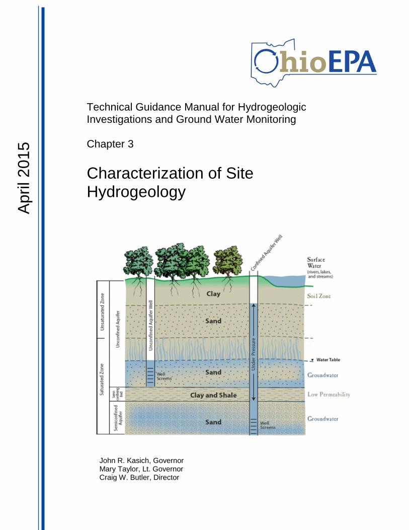
Technical Guidance Manual for Hydrogeologic Investigations and Ground Water Monitoring Chapter 3

Characterization of Site Hydrogeology

April 2015

John R. Kasich, Governor Mary Taylor, Lt. Governor Craig W. Butler, Director

TGM Chapter 3: Site Hydrogeology 3-ii Revision 2, April 2015

CHAPTER 3

Characterization of Site Hydrogeology

April 2015

Revision 2

Ohio Environmental Protection Agency Division of Drinking and Ground Waters

P.O. Box 1049 50 West Town Street, Suite 700

Columbus, Ohio 43216-1049 Phone: (614) 644-2752 epa.ohio.gov/ddagw/

TECHNICAL GUIDANCE MANAUAL FOR HYDROGEOLOGIC

INVESTIGATIONS AND GROUND WATER MONITORING

TGM Chapter 3: Site Hydrogeology 3-iii Revision 2, April 2015

TABLE OF CONTENTS

TABLE OF CONTENTS ................................................................................................................. iii PREFACE ....................................................................................................................................... v CHANGES FROM THE FEBRUARY 2006 TGM ............................................................................ vi 1.0 PRELIMINARY EVALUATIONS ................................................................................................ 2 2.0 FIELD METHODS TO COLLECT HYDROGEOLOGIC SAMPLES AND DATA ......................... 5

2.1 DIRECT TECHNIQUES ....................................................................................................... 5 2.1.1 Boring/Coring ................................................................................................................ 5 2.1.2 Test Pits and Trenches ................................................................................................. 7 2.1.3 Pumping and Slug Tests ............................................................................................... 7 2.1.4 Tracer Tests .................................................................................................................. 7 2.1.5 Ground Water Level Measurements .............................................................................. 9

2.2 SUPPLEMENTAL TECHNIQUES ...................................................................................... 11 2.2.1 Geophysics ................................................................................................................. 11 2.2.2 Cone Penetration Tests .............................................................................................. 11 2.2.3. Aerial Imagery ............................................................................................................ 12

3.0 HYDROGEOLOGIC CHARACTERIZATION............................................................................ 12 3.1 STRATIGRAPHY ............................................................................................................... 13 3.2 DESCRIPTION AND CLASSIFICATION OF UNCONSOLIDATED MATERIALS ............... 13

3.2.1 Classification Systems ................................................................................................ 13 3.2.2 Texture (Particle Size, Particle Shape and Packing) ................................................... 15 3.2.3 Plasticity...................................................................................................................... 15 3.2.4 Toughness .................................................................................................................. 16 3.2.5 Dilatancy ..................................................................................................................... 17 3.2.6. Typical Field USCS Fine Grained Soil Classes in Ohio .............................................. 17 3.2.7 Consistency ................................................................................................................ 17 3.2.8 Color ........................................................................................................................... 18 3.2.9 Moisture Content ......................................................................................................... 18 3.2.10 Consistency .............................................................................................................. 19 3.2.11 Sedimentary Structures and Depositional Environment ............................................. 20

3.3 DESCRIPTION AND CLASSIFICATION OF CONSOLIDATED MATERIALS ..................... 22 3.4 FRACTURING .................................................................................................................... 23 3.5 ANTHROPOGENIC INFLUENCE ....................................................................................... 26 3.6 GROUND WATER OCCURRENCE ................................................................................... 27

3.6.1 Flow Direction ............................................................................................................. 28 3.6.2 Hydraulic Gradient ...................................................................................................... 35 3.6.3 Porosity/Effective Porosity .......................................................................................... 35 3.6.4 Hydraulic Conductivity................................................................................................. 36 3.6.5 Intrinsic Permeability/Coefficient of Permeability ......................................................... 42 3.6.6 Transmissivity ............................................................................................................. 43 3.6.7 Storage Coefficient, Specific Storage and Specific Yield ............................................. 43 3.6.8 Flow Rate .................................................................................................................... 43 3.6.9 Saturated Zone Yield .................................................................................................. 44

4.0 GROUND WATER USE DETERMINATION ............................................................................ 45 4.1 PUBLICLY AVAILABLE RECORDS ................................................................................... 45 4.2 SURVEYS .......................................................................................................................... 45 4.3 OTHER LINES OF EVIDENCE .......................................................................................... 45

5.0 ANALYSIS AND PRESENTATION OF HYDROGEOLOGIC INFORMATION .......................... 46 5.1 WRITTEN DESCRIPTION .................................................................................................. 46 5.2 RAW DATA ........................................................................................................................ 47 5.3 CROSS SECTIONS ........................................................................................................... 48

TGM Chapter 3: Site Hydrogeology 3-iv Revision 2, April 2015

5.4 MAPS ................................................................................................................................. 48 5.5 METHODOLOGY ............................................................................................................... 49

6.0 REFERENCES ........................................................................................................................ 50

TGM Chapter 3: Site Hydrogeology 3-v Revision 2, April 2015

PREFACE The subject of this document is techniques to characterize hydrogeology beneath a site. It is part of a series of chapters incorporated in Ohio EPA’s Technical Guidance Manual for Hydrogeologic Investigations and Ground Water Monitoring (TGM), which was originally published in 1995. Ohio EPA now maintains this guidance as a series of chapters rather than as an individual manual. These chapters can be obtained at epa.ohio.gov/ddagw/tgmweb.aspx.

The TGM identifies technical considerations for performing hydrogeologic investigations and ground water monitoring at potential or known ground water pollution sources. The purpose of the guidance is to enhance consistency within the Agency and inform the regulated community of the Agency’s technical recommendations and the basis for them.

Ohio EPA utilizes guidance to aid regulators and the regulated community in meeting laws, rules, regulations and policy. Guidance outlines recommended practices and explains their rational. The methods and practices described in this guidance are not intended to be the only methods and practices available to an entity for complying with a specific rule. Unless following the guidance is specifically required within a rule, the agency cannot require an entity to follow methods recommended by the guidance. The procedures used to meet requirements usually should be tailored to the specific needs and circumstances of the individual site, project, and applicable regulatory program, and should not comprise a rigid step-by-step approach that is utilized in all situations.

TGM Chapter 3: Site Hydrogeology 3-vi Revision 2, April 2015

CHANGES FROM THE FEBRUARY 2006 TGM Ohio EPA’s Technical Guidance Manual for Hydrogeologic Investigations and Ground Water Monitoring (TGM) was first finalized in 1995. Chapter 3 (Characterization of Site Hydrogeology) was subsequently updated in October 2006. This is the second revision to the chapter. Section numbers were added to make the document easier to read. References were updated, in particular, the references to ASTM standards. The appendix listing out geophysical techniques was removed. The Agency decided that it would maintain a Geophysical Chapter (Chapter 16- Application of Geophysical Methods for Site Characterization), thus did not need to repeat the information. Additional information has been added on

Description and Classification of Unconsolidated Deposits. In particular, on sedimentary structures (3.3.11), toughness (3.2.4), and dilatancy (3.3.5). In addition, some of the major USCS for fine grain classifications found in Ohio were identified.

Environmental and Injected Tracers (2.1.4)

Ground water level measurements. (2.1.5). Incorporated the guidance from the supplementary document Monitoring Well Fixed Survey Elevation Reference Point (March 23, 2010).

TGM Chapter 3: Site Hydrogeology 3-1 Revision 2, April 2015

CHAPTER 3 CHARACTERIZATION OF SITE HYDROGEOLOGY

Investigations of existing or potential ground water pollution sources should include an adequate characterization of site hydrogeology. Typically, an evaluation includes a three-dimensional assessment of the underlying geologic materials and the movement of ground water within the materials. This information is needed to assess whether ground water has been impacted by pollution sources, determine the extent of contamination, and determine whether contaminants have reached a receptor. The scope of an investigation should be based on its objectives, any regulatory requirements, and site-specific conditions. The following approach should be used:

Define the requirements and technical objectives. The requirements and objectives are dependent on the objectives of the investigation and may be dictated by the regulatory program. An entity may be evaluating the hydrogeology of an area to: 1) determine if it is compatible with its intended use; 2) ascertain the impact of a past, existing, or proposed activity on the ground water resources of the region; and/or 3) provide a basis for a site clean-up program. Project requirements and objectives should be discussed with the appropriate Agency representative prior to initiating studies.

Perform a preliminary evaluation. A preliminary evaluation is a comprehensive review of existing information, including regional and site-specific hydrogeologic data. The evaluation should be utilized to develop a preliminary conceptual model.

Collect site-specific hydrogeologic data. The results of the preliminary evaluation, along with project requirements and technical objectives, should be utilized to design the first phase of a site-specific investigation. Information gathered can be utilized to refine the conceptual model and assist in developing additional phases, if needed. In general, the characterization is considered complete when enough information has been collected to satisfy regulatory requirements and the potential pathways for contaminant migration have been defined and characterized. Prior to performing any field work, a site safety plan may need to be developed in accordance with the Occupational Safety and Health Administration (OSHA) requirements of 29 CFR 1910.120.

When conducting hydrogeologic investigations, the user may want to consider approaches as discussed in the following U.S.EPA programs to focus the assessment and promote efficient collection of data.

Guidance on Systematic Planning Using the Data Quality Objectives Process EPA QA/G-4. epa.gov/quality/qs-docs/g4-final.pdf

Guidance for the Data Quality Objectives Process EPA QA/G-4. orau.org/ptp/PTP%20Library/library/EPA/QA/g4.pdf

Dynamic Workplans epa.gov/superfund/programs/dfa/dynwork.htm

Triad: triadcentral.org/over/index.cfm

TGM Chapter 3: Site Hydrogeology 3-2 Revision 2, April 2015

1.0 PRELIMINARY EVALUATIONS Characterization should begin with a review of available regional and site-specific hydrogeologic information. Wastes or constituents of concern should also be investigated. This preliminary evaluation should serve as the basis for the conceptual model and field investigation. Information that may be gathered includes, but is not limited to:

Logs from private, public, industrial, agricultural, monitoring, oil, gas, and injection wells.

Logs from building or quarry activities.

Records documenting local influences on ground water flow and use (for example, on- or off-site production wells, irrigation or agricultural use, river stage variations and land use patterns, etc.).

Geologic and ground water data obtained from various reports for the area or region.

Topographic, geologic, soil, hydrogeologic and geohydrochemical maps and aerial photographs.

Information may be obtained from the sources listed below. Division of Mineral Resources Management, Ohio Department of Natural Resources (ODNR). (2045 Morse Road, Building H-3, Columbus, Ohio 43229 Phone: (614) 265-6633 Web: minerals.ohiodnr.gov). The Division of Mineral Resource Management is comprised of the following departments: Industrial Minerals, Coal Mining, Mine Safety, Shale Development, and Abandoned Mined Lands. The Department of Industrial Minerals has hydrogeologic reports for new and existing quarry operations. This information may contain useful data on quarry geology and potential dewatering effects on local wells, including pumping test data and aquifer characteristics. In addition, each quarry must file an annual water withdrawal report with the ODNR Division of Water, which can provide an estimate of ground water pumpage. The Department of Coal Mining administers and regulates both surface and deep mines and has permits and hydrogeologic data on file, possibly in addition to what is available with the Division of Geological Survey. Division of Oil and Gas Resources, Ohio Department of Natural Resources (ODNR). (2045 Morse Road, Building F-2, Columbus, Ohio 43229 Phone: (614) 265-6922 Web: oilandgas.ohiodnr.gov). The Division of Oil and Gas Resources has oil and gas well completion records, which may provide general information on bedrock geology. Borehole geophysical logs may also be available. Division of Soil and Water Resources, ODNR (2045 Morse Road, Building B-3, Columbus, Ohio 43229 Phone: (614) 265-6610 Web: soilandwater.ohiodnr.gov). The Ground Water Mapping and Technical Services Section is responsible for the quantitative evaluation of ground water resources. Specific functions include ground water mapping, administration of Ohio's ground water well log and drilling report law, and special assistance to municipalities, industries, and the general public regarding local geology, well drilling and development, and quantitative problem assessment. Ground water availability maps have been published. These maps can be downloaded from the Division’s internet site or a paper copy can be ordered. The Division's file of well logs contains submitted records for water supply and monitoring wells. Well logs are available online, or arrangements can be made to search the well log files. The Division is also involved in drafting pollution potential maps (often referred to as DRASTIC maps), which can be used in general planning. These maps are available online. Potentiometric surface maps are also available for some

TGM Chapter 3: Site Hydrogeology 3-3 Revision 2, April 2015

counties. These maps can be used for general planning. Other available information includes ground water reports and bulletins. The Water Use and Planning Unit operates continuous ground water level recorders within about 140 observation wells. The Water Inventory Program continually compiles and stores ground water elevations, precipitation data, water storage, palmer drought indices and stream flow data. The Unit characterizes the condition of Ohio’s ground water resources through continuous monitoring and evaluating long-term trends in ground water level fluctuations throughout the state’s various aquifer systems. Division of the Geological Survey, ODNR (2045 Morse Road, Building C, Columbus, Ohio 43229 Phone: (614) 265-6576 Web: geosurvey.ohiodnr.gov). The Division of the Geological Survey, ODNR, is responsible for the collection and dissemination of information relating to bedrock and surficial geology. Through mapping, core drilling, and seismic interpretation, the Survey compiles maps and inventories of bedrock and surficial materials and offers advice concerning mining-related issues. Published reports regarding bedrock and glacial geology are available for many counties. Additional information on bedrock geology is available from files of logs produced for oil and gas exploration. The USGS 7½ minute topographic maps are available from the Survey. These maps can provide basic information on spatial location of buildings (for example, homes, schools, factories, etc.), roads and streams, surface elevations and topography, and general land use. These maps and reports can be ordered from the Division, and some are available online. The ODNR Division of Geological Survey Horace R. Collins Laboratory (HRCL), located at Alum Creek State Park in Delaware County, houses a collection of geologic samples (for example, rock and unconsolidated glacier sediments) that can be reviewed by the public by appointment. It also has aerial photographs from 1947 to 1979. Natural Resources Conservation Services (NRCS), United States Department of Agriculture (200 North High Street, Room 522, Columbus, Ohio 43215 Phone: (614) 255-2472 Web: nrcs.usda.gov/wps/portal/nrcs/site/oh/home). The NRCS (formerly Soil Conservation Services) provides leadership in a partnership effort to help private land owners and managers conserve their soil, water and other natural resources. One source of information useful for preliminary investigations is the soil surveys. These maps illustrate major soil types and their agricultural and engineering attributes. The NRCS has digitized many of the surveys (Soil Survey Geographical [SSURGO] database) and they are available online for almost all counties in Ohio. Maps also are available through the ODNR, Division of Soil and Water Resources. United States Geological Survey (USGS), Ohio Water Science Center (6480 Double Tree Avenue, 43229 Phone: (614) 430-7700 Web: oh.water.usgs.gov). The mission of the USGS Water Resources Division is to provide the hydrologic information and understanding needed for the optimum utilization and management of the Nation's water resources for the overall benefit of the United States. A summary of the Survey's program in Ohio can be found in USGS Fact Sheet 2014-3097 (2014). Responsibilities include collection of the basic data needed for determination and evaluation of the quantity, quality, and use of Ohio's water resources, conductance of analytical and interpretive water-resources appraisals describing the occurrence, availability, physical, chemical and biological characteristics of surface water and precipitation, and implementation of similar appraisals associated with ground water. The USGS publishes an annual series of reports titled "Water Resources Data-Ohio, Volume 1 and 2" in which the hydrologic data collected during each water year are presented. The USGS, National Center for Earth Resources Observation and Science (EROS) is the primary source for country-wide aerial photography. For a list of USGS publications per county, see oh.water.usgs.gov/reports/pub-biblio.html.

TGM Chapter 3: Site Hydrogeology 3-4 Revision 2, April 2015

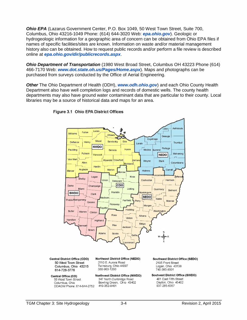
Ohio EPA (Lazarus Government Center, P.O. Box 1049, 50 West Town Street, Suite 700, Columbus, Ohio 43216-1049 Phone: (614) 644-3020 Web: epa.ohio.gov). Geologic or hydrogeologic information for a geographic area of concern can be obtained from Ohio EPA files if names of specific facilities/sites are known. Information on waste and/or material management history also can be obtained. How to request public records and/or perform a file review is described online at epa.ohio.gov/dir/publicrecords.aspx. Ohio Department of Transportation (1980 West Broad Street, Columbus OH 43223 Phone (614) 466-7170 Web: www.dot.state.oh.us/Pages/Home.aspx). Maps and photographs can be purchased from surveys conducted by the Office of Aerial Engineering. Other The Ohio Department of Health (ODH), www.odh.ohio.gov) and each Ohio County Health Department also have well completion logs and records of domestic wells. The county health departments may also have ground water contaminant data that are particular to their county. Local libraries may be a source of historical data and maps for an area.

TGM Chapter 3: Site Hydrogeology 3-5 Revision 2, April 2015

2.0 FIELD METHODS TO COLLECT HYDROGEOLOGIC SAMPLES AND DATA This section covers various direct and supplemental field tools and methodologies used to characterize the subsurface materials and ground water conditions present within a given area by sampling or in-situ testing. The extent of characterization and specific methods used will be determined by the project objectives, regulatory requirements and the data quality objectives of the investigations. Specific hydrogeologic information that should be collected and appropriate techniques (both field and laboratory) to collect the data are covered in the Hydrogeologic Characterization Section (Page 3-14). 2.1 DIRECT TECHNIQUES Hydrogeologic site characterization generally includes the collection of subsurface samples from borings or excavations. These samples are needed to describe and classify subsurface materials and to evaluate subsurface conditions and stratigraphy. Other direct techniques include aquifer testing, environmental and injected tracers, and ground water level measurements. 2.1.1 Boring/Coring The objectives of a subsurface boring/coring program1 are to collect data to characterize subsurface conditions. Available geologic and hydrogeologic information should be used to develop a preliminary conceptual model of the subsurface conditions. This will aid in selecting appropriate boring locations and depths. Supplemental techniques such as geophysical or aerial imagery may be helpful in evaluating the number, location and depth of borings. Information about designing a subsurface boring/coring program is discussed below. Details on how to describe and classify the material is discussed on page 3-15. Subsurface investigations include the collection of soil and unconsolidated materials using a split-barrel sampler, thin-walled (Shelby tube) sampler, or continuous sampler, and the collection of rock using a coring device. These samples are used to determine the physical and chemical properties of the subsurface materials. The type of drilling equipment and sampling methods depends on the material, nature of the terrain, intended use of the data, depth of exploration, and prevention of cross-contamination. Detailed information pertaining to drilling and sampling is covered in Chapter 6 (Drilling and Subsurface Sampling) and Chapter 15 (Use of Direct Push Technologies for Soil and Ground Water Sampling). The number, location, depth, and spatial distribution (density) of borings depends on subsurface complexity, the size of the site being investigated, and on the importance of understanding the site stratigraphy and other conditions with respect to the investigation objectives. The locations of individual borings should depend on site hydrogeology, geomorphic features, spatial location of waste (or suspected waste), and anthropogenic (human-made) impediments such as underground utility lines. In general, the density should be greater when characterizing geology that is more complex. Table 3.1 lists factors that should be considered. Exploration should be deep enough to identify all strata that might be significant in assessing the environmental conditions. At a minimum, initial borings should be sampled continuously. Once control has been established, the continuous approach may no longer be necessary. It should be noted that the proper interval may not be constant and may depend on the target zone(s) of interest.

1Borings not to be converted into wells must be properly sealed (See Chapter 9).

TGM Chapter 3: Site Hydrogeology 3-6 Revision 2, April 2015

Borings should not be installed through waste material; however, in some instances this is unavoidable. Authorization from Ohio EPA is required before drilling through waste (ORC 3734.02(H))2. The applicable regulatory program should be contacted for appropriate authorization. Care should be taken when drilling into confining units so that the borehole does not create a conduit for migration of contaminants between hydraulically separated saturated zones. Two approaches for drilling through confining layers should be considered:

If sampling and analytical data are available, drill initially in less contaminated or uncontaminated areas. These borings could penetrate the confining zone to characterize deeper units. At a minimum, borings upgradient of the source could be drilled through the possible confining layer to characterize site geology. The appropriateness of this approach should be evaluated on a site-specific basis.

Drill using techniques (for example, telescoped casing) that minimize potential cross-contamination, particularly from dense non-aqueous phase liquids (DNAPLs). Telescoped casing involves drilling partially into a confining layer, installing an exterior casing, sealing the annular space in the cased portion of the borehole, and drilling a smaller diameter borehole through the confining layer (See Chapter 6).

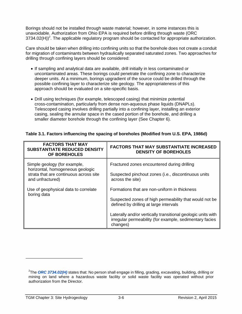
Table 3.1. Factors influencing the spacing of boreholes (Modified from U.S. EPA, 1986d)

FACTORS THAT MAY SUBSTANTIATE REDUCED DENSITY

OF BOREHOLES

FACTORS THAT MAY SUBSTANTIATE INCREASED DENSITY OF BOREHOLES

Simple geology (for example, horizontal, homogeneous geologic strata that are continuous across site and unfractured) Use of geophysical data to correlate boring data

Fractured zones encountered during drilling Suspected pinchout zones (i.e., discontinuous units across the site) Formations that are non-uniform in thickness Suspected zones of high permeability that would not be defined by drilling at large intervals Laterally and/or vertically transitional geologic units with irregular permeability (for example, sedimentary facies changes)

2The ORC 3734.02(H) states that: No person shall engage in filling, grading, excavating, building, drilling or

mining on land where a hazardous waste facility or solid waste facility was operated without prior authorization from the Director.

TGM Chapter 3: Site Hydrogeology 3-7 Revision 2, April 2015

2.1.2 Test Pits and Trenches Pits and trenches may be cost-effective in characterizing shallow, unconsolidated materials and determining depth to shallow bedrock or a shallow water table. The depth limit is dependent on the reach of the backhoe/excavator (for example, 15 to 20 feet), and any safety issues that need to be addressed (for example, stable slopes, and sidewalls, buried structures, etc.). Depth is also limited to a few feet below the water table. A pumping system may be necessary to control water levels. Authorization from Ohio EPA is required before drilling through waste (ORC 3734.02(H)). Test pit/trench locations should be accurately surveyed with the dimensions noted. Field logs should contain a sketch of pit conditions, approximate surface elevation, depth, method of sample acquisition, soil and rock description, ground water levels, and other pertinent information such as waste material encountered or organic gas or methane levels (if monitored). Any significant features should be photographed (scale should be indicated). Backfilling should be completed to prevent the pit/trench from acting as a conduit. One method is to use a soil-bentonite mixture prepared in proportions that represent permeability equal to or less than original conditions. The material should be placed to prevent bridging and subsequent subsidence. Since proper sealing is difficult, pits/trenches should be limited to the vicinity of a proposed waste disposal site (i.e., within the area to be excavated) or adjacent to suspected areas of contamination. Disadvantages of test pits/trenches include potential handling/disposal of contaminated soils and water (see Chapter 6), disruption of business activities, and safety hazards. If entry into excavations is necessary, several Occupational Safety and Health Administration (OSHA) regulations must be followed. The reader should refer to 29 CFR 1926, 29 CFR 1910.120, and 29 CFR 1910.134. A detailed description of test pit/trench programs can be found in A Compendium of Superfund Field Operations Methods: Volume 1 (U.S. EPA, 1987). 2.1.3 Pumping and Slug Tests Pumping and slug tests are used to define the hydraulic characteristics of ground water zones and confining layers that lie above or below. These properties may also be needed to predict the ground water flow rate and design effective ground water remediation systems. Slug tests can provide information about the hydraulic conductivity of a layer. Pumping tests can provide information on hydraulic conductivity, interconnectiveness between ground water zones, heterogeneity, and boundary conditions. One drawback of long-term pumping tests is the handling and disposing of the large volume of water that is generated. Information on how to design pumping and slug tests is provided in Chapter 4. 2.1.4 Tracer Tests Tracer tests can help quantify the hydrogeologic characteristics of the ground water. Tracers can be naturally-occurring, such as heat carried by hot-spring waters; globally-produced from anthropogenic sources, such as an above-ground nuclear weapon detonation test; or intentionally injected3, such as dyes. Naturally-occurring and globally-produced types often are referred to as environmental tracers. If sufficient information is collected, tracers may be used to determine hydraulic conductivity (K), porosity, dispersivity, chemical distribution coefficients, flow direction, flow rate, sources of

3If fluids are injected into the subsurface, a Class V well operating permit may be required. Ohio EPA,

Division of Drinking and Ground Waters, Underground Injection Control Unit (UIC) has jurisdiction over review and issuance of these permits. If you have any questions concerning Class V wells, please contact the Ohio EPA-DDAGW, UIC unit. epa.ohio.gov/portals/28/documents/uic/classvinventory.pdf.

TGM Chapter 3: Site Hydrogeology 3-8 Revision 2, April 2015

recharge, and ground water age. More information on tracer tests can be found at the USGW webpage: toxics.usgs.gov/topics/tracer_tests.html. 2.1.4.1 Injected Tracers Injected tracer tests are used to "trace" the path of flowing water and may be conducted in pipelines, lakes, rivers, and ground water. An injected tracer should have a number of properties to be useful. It should be non-reactive. This means the mass of the tracer is not lost through reaction or partitioning into differing phases (vapor, solids). Thus, the only solute transport processes affecting a non-reactive tracer are advection and dispersion. The tracer should also be relatively inexpensive and easily sampled, analyzed and detected. Any injected tracer should be non-toxic and should be used with careful consideration of possible health effects. The tracer should not be related to known site contamination. The most commonly injected tracers used in ground water studies are:

fluorescent dyes such as fluorescein and rhodamine-WT, and

halides such as chloride, bromide and iodide.

Information on types of injected tracers and tracer tests can be found in Field et al., 1995; Aley, 2002; Weight and Sonderegger, 2001; Boulding, 1995; U.S. EPA, 1996; and U.S. EPA, 2003 - cfpub.epa.gov/ncea/cfm/recordisplay.cfm?deid=56892#Download. 2.1.4.2 Environmental Tracers Isotopes, which are atoms of the same element that differ in mass because of a difference in the number of neutrons in the nucleus, serve as valuable tracers. The naturally-occurring elements give rise to more than 1,000 stable and radioactive isotopes, commonly referred to as environmental isotopes. These can be used to identify the origin of ground water, determine its relative age (i.e., length of time it has been out of contact with the atmosphere), and determine if saturated zones are interconnected. This can be important when trying to determine how long it may take a potential contaminant to reach a ground water zone or receptor. Age-dating shows which wells draw more recently recharged ground water and, therefore, may be more susceptible to contamination from the surface. Older water may be less contaminated because it has either been shielded from contact with pollutants or has had more time for natural processes to reduce or eliminate contamination. All dating techniques have limitations. Greater confidence in apparent age will be realized as multiple dating techniques are applied to the same sample. Isotopes and/or isotope ratios that may assist in evaluating the ground water include:

Tritium H3, which is used to determine if ground water was recharged prior to 1954 or after 1954.

Oxygen-18/oxygen -16 ratio (18O/16O), which indicates if ground water is pre-Holocene or post-Holocene in age. The calculated mass can yield information about the temperature at the time of its formation (NASA website-Paleoclimatology at earthobservatory.nasa.gov/Features/Paleoclimatology_OxygenBalance/).

Relative fractions of deuterium (δH2) and oxygen-18 (δ18O) (Fetter, 2001). Where glacial tills are wide-spread, vertical profiles of δH2 and δ18O in pore waters are valuable natural isotopes

that yield independent information on hydraulic properties and solute transport mechanism. The ratio can also be helpful in age dating the ground water (Kazemi, et al., 2006).

TGM Chapter 3: Site Hydrogeology 3-9 Revision 2, April 2015

Carbon -14 (14C), which is used to estimate the relative age of ground water.

Tritium (3H)/Helium-3 (3He) ratio. When 3He is due to decay of 3H and can be separated from that due to other sources, parent-daughter ratios enable accurate estimations of ground water age. Such information can be useful to estimate ground water residence and flow velocities (Solomon and Cook, 2000).

Chlorofluorocarbons (CFCs) are stable, synthetic, halogenated alkanes, developed in the early 1930s as an alternative to ammonia sulfur dioxide refrigeration. They provide tracer and dating tools of younger water (50-year time scale.) Additional information on the application of chlorofluorocarbons can be found in Plummer and Busenberg (2000).

The complexities of natural systems together with the use criteria for tracers makes selection and use almost as much of an art as it is a science (U.S. EPA, 1991). The potential chemical and physical behavior of the tracer in the ground water must be understood. The type of medium and flow regime should also be considered. It is beyond the scope of this document to detail the proper use, selection and design of tracers. Sources of information include: Kazemi et al., (2006), Cook and Herczeg (editors, 2000), Alley (1993), Davis et al. (1985), and the USGS National Research Program: water.usgs.gov/nrp/groundwater.html. 2.1.5 Ground Water Level Measurements Water level measurements in wells are needed to: determine ground water flow and hydraulic gradients; interpret the amount of water available for withdrawal; and determine the effects of natural and anthropogenic (human-induced) influences on flow. Reliable water table and potentiometric surface maps are essential to any hydrogeologic investigation and the design, installation and maintenance of an adequate ground water monitoring system. Accurate static water level elevation measurements from monitoring wells and piezometers must be obtained to create these maps. The number and location of observation wells are critical to any water level data program. Selection of the location and depth should be based on hydrogeologic/geologic characteristics of the area, physical boundaries, anthropogenic influences and contaminant characteristics. Areas with multiple ground water zones may necessitate well clusters. 2.1.5.1 Surveying the Monitoring Wells To enable consistent and accurate static water level elevation measurements, each monitoring well should have a surveyed elevation reference point that is consistently used when measuring water levels and total well depth. Typically, this point is on the north side of the inner well casing and should be clearly visible with a notch or some other permanent mark. If the surveyed reference point is made on a removable well cap from which a pump is suspended within the well, then the reference point should be next to the water level measuring hole in the well cap and the orientation and depth of the well cap on the well casing should be marked. If the well cap is removed, it should be replaced in the same place and orientation as before it was removed based on the marks on the casing. The level of accuracy needed for the measured reference point depends on any regulatory requirements and the water level data quality objectives. In addition, the accuracy is dependent on the type, accuracy, and precision of the surveying method used. Some regulations require water level measurements to be accurate to the nearest 0.01 foot; and therefore, may necessitate the elevation reference point be established by a licensed surveyor. If an accuracy of ±0.01 is not needed, then the reference point may be established by a qualified professional and a Global

TGM Chapter 3: Site Hydrogeology 3-10 Revision 2, April 2015

Positioning System (GPS) elevation survey with accuracies up to ±0.04 may be adequate. The method used and the accuracy should be documented. Regardless, the surveyed referenced elevation error should be equal or less than the error of water level measurement data to properly evaluate ground water flow direction. The established elevation of the reference point is generally based on mean sea level. Another datum can be used as long as the entire monitoring well network is tied to it. Both the elevation datum and the x, y coordination system used should be documented. Total depth measurements also need to be taken at times to determine if the well is being maintained properly. The elevation of an individual well should be re-surveyed when it:

Has been damaged (for example, by vehicle/heavy equipment) and repaired.

Shows evidence of frost heaving.

Has been altered or modified (well casing cut shorter or extended).

Shows evidence of settling over time. In some cases, the entire network of wells may need to be resurveyed when there are unexplainable shifts in ground water flow direction that cannot be attributed to a single well. This is particularly true when the ground water table or potentiometric surface is flat and slight changes in elevation (even hundredths of a foot) could change the interpretation of flow direction and gradient. The re-surveying needs to be conducted using the same datum system established for the original monitoring well network. If monitoring wells have been installed and surveyed over time during successive phases of investigations at a site, it is recommended that a single elevation survey be performed for the entire network to ensure that the reference point elevations are accurate. 2.1.5.2 Measuring and Recording Water Levels Water levels can be collected manually or by continuous recorders. In addition to measurements from wells, information from springs, seeps, rivers, ponds and lakes may also be useful if they are shown to be hydraulically connected to the ground water zone being studied. Manual water level measurements are generally obtained with electrical probes or transducers and are a component of any ground water sampling program (See Chapter 10: Ground Water Sampling). When measuring manually, water levels from all wells should be taken in as short a time as possible. Influences, such as recharge from precipitation, barometric pressure changes, water withdrawal, artificial recharge (for example, injection wells, leakage around a poorly sealed well) and heavy physical objects that compress the sediments (for example, passing train), may change the water level in wells and affect the interpretation of ground water flow. However, often wells within a study area do not change significantly in a short time. It is often necessary to monitor the continuous fluctuation of water. Continuous measurement methods include: a mechanical float recording system; electromechanical iterative conductance probes connected to chart recorders; and transducers with data loggers (Dalton et al., 2006). In general, Ohio EPA recommends that water level measurements be provided in a table and include the date and time of the measurement. The values should also be included on potentiometric maps. ASTM 6000 provides graphical and tabular methods for presenting ground water level information.

TGM Chapter 3: Site Hydrogeology 3-11 Revision 2, April 2015

2.2 SUPPLEMENTAL TECHNIQUES Supplemental techniques such as geophysics, cone penetration tests, and aerial imagery can be used to help guide and implement a boring program and assist in defining site hydrogeology. Use of these techniques can be cost-effective, as they may reduce the number of borings necessary. 2.2.1 Geophysics Geophysics may be used to augment direct field methods or guide their implementation. Geophysical measurements supplement borehole and outcrop data and assist in the interpolation between boreholes. Geophysics can also be useful in identifying surface drilling hazards and contamination. Geophysical techniques can be categorized as either surface or borehole. Surface methods are generally non-intrusive. Borehole methods require that wells or borings exist so that tools can be lowered into the subsurface. Direct push (DP) technology probes have been fitted with sensors and can provide information rapidly (See Chapter 15: Use of Direct Push Technologies for Soil and Ground Water Sampling). Surface techniques can provide information on depth to bedrock, types and thicknesses of geologic material, presence of fracture zones and solution channels, structural discontinuities, and depth to the water table. They are also useful in locating drilling hazards (for example, buried drums and pipelines). Types of surface geophysical techniques include: ground penetrating radar, electromagnetic induction, electrical resistivity, seismic refraction, seismic reflection and magnetic surveys. Borehole techniques can be used to obtain information on material type, stratigraphy, formation and aquifer properties, ground water flow, borehole fluid characteristics, contaminant characteristics and borehole/casing conditions. They may indicate areas of high porosity and hydraulic conductivity, ground water flow rates and direction, subsurface stratigraphy, lithology of bedrock units and chemical and physical characteristics of ground water. Borehole methods include nuclear logs (natural gamma, gamma-gamma, neutron-neutron), non-nuclear logs and physical logs (temperature, fluid conductivity, fluid flow and caliper.) This chapter does not describe the various geophysical methods, however, a list of various methods helpful to characterize site hydrogeology, along with techniques that may help identify contaminants and contaminant sources (buried drums, pipelines, etc.) can be found in Chapter 11 - Application of Geophysical Methods for Site Characterization. All geophysical methods require site conditions that provide contrast in the subsurface properties being measured. Depending on the method, implementation may be affected by interferences such as metal fences, power lines, FM radio transmissions or ground vibrations. Data collected and interpreted from geophysical surfaces require skilled personnel familiar with the principles and limitations of the method being used. 2.2.2 Cone Penetration Tests Cone penetration testing (CPT) is applicable where formations are uncemented and unlithified; free from impenetrable obstructions such as rock ledges, hardpans, caliche layers, and boulders; and conducive to penetration with minimal stress to the testing equipment (Smolley and Kappmeyer, 1991). The technique consists of advancing a mechanical or electronic rod to determine the end-bearing and side friction components of resistance to penetration (ASTM D3441, ASTM D5778).

TGM Chapter 3: Site Hydrogeology 3-12 Revision 2, April 2015

These two parameters typically are different for coarse-grained and clayey soils, making the CPT a particularly useful tool for defining and correlating the occurrence of sands and gravels versus clays and silts (Smolley and Kappmeyer, 1991). Mechanical cone penetrometers are addressed in ASTM D3441, while electronic cone penetrometers are addressed in ASTM D5778. The mechanical penetrometer operates incrementally using a telescoping tip, which results in no movement of the push rod. Electronic cone penetrometers use force transducers located in a non-telescoping penetrometer tip to measure penetration resistance. Other sensors--such as piezometric head transducers, pH indicators, and detectors for petroleum hydrocarbons--may also be included in the cone to provide additional information. At sites where the technique is applicable, CPT surveys can provide a continuous vertical profile of subsurface stratigraphy and indications of permeability. In all cases, the data needs to be compared with information from borings and geologic material sampling. Proper interpretation of cone penetrometer data requires comparison with a logged soil boring (geologic material description) at a minimum of one location per area investigated. Additional information on the use of CPT for environmental site investigations is presented in U.S. EPA (1997). 2.2.3. Aerial Imagery Aerial imagery, if they can be reasonably obtained, can be used to help: 1) identify rock and surface soil types, geomorphological features and the nature and extent of joint and fault patterns; 2) approximate stream flow, evapotranspiration, infiltration and runoff values; and 3) map topographic features such as streams, seeps and other surface waters not readily apparent from ground level. Comparing old and new topographic maps and aerial photographs can help ascertain changes over time such as those caused by cut and fill activities, drainage alteration and land use (Benson, 2006). Vegetative stress identified in aerial imagery may indicate the location of a contaminant plume. Aerial imagery can be used for fracture analysis. Fracture traces are surface expressions of joints or faults. Fractures may provide pathways for ground water and contaminants. The greatest yields may be located at the intersection of two fracture traces. Therefore, fracture trace analysis may help identify appropriate boring and monitoring well locations. Fracture trace analysis is covered on page 3-31. Aerial photographs may be obtained from the U.S. Department of Agriculture, Agriculture Stabilization and Conservation Service (ASCS) offices in each county. They may also be available through the Ohio Department of Transportation, Office of Aerial Engineering. Documentation of analysis of aerial photographs should include source, date, and type of photograph. Internet sources of aerial maps are also available (for example, Google Earth®). Information on the use of aerial photography can be found in Nielsen et al. (2006).

3.0 HYDROGEOLOGIC CHARACTERIZATION

A proper evaluation of site hydrogeology should include, but not be limited to, identification of the lateral and vertical extent of subsurface materials, the type of materials, the geological influences that may control ground water flow (for example, high permeability zones, fractures, fault zones, fracture traces, buried stream deposits, etc.), and the occurrence and use of ground water. As indicated above, direct information is collected through borings, test pits, and field and laboratory identification of subsurface materials. Supplemental information (for example, geophysical data) can be used to augment the direct methods or to guide their implementation, but should not be used as a substitute.

TGM Chapter 3: Site Hydrogeology 3-13 Revision 2, April 2015

3.1 STRATIGRAPHY Stratigraphy is the study of the formation, composition, sequence and correlation of unconsolidated materials and consolidated materials (rock). It includes formation designation, age, thickness, areal extent, composition, sequence and correlation. In effect, stratigraphy defines the geometric framework of the ground water flow system. Therefore, knowledge of the local stratigraphy is necessary to define the hydrogeologic framework and identify pathways of chemical migration and extent of migration. Necessary determinations include zones that may restrict movement of ground water (confining zones) and zones that enhance ground water movement. Existing information such as driller’s logs and regional information can provide information on stratigraphy. This information may be helpful in designing a site-specific drilling program. Sample collection from borings and cores is needed to determine whether the subsurface layers have the ability to transmit water or prohibit the movement of water by serving as a confining layer. Geophysical methods can be used to direct or augment the characterization of stratigraphy. Thick, continuous layers of unfractured clay, fine silt, or shale may retard flow. They are generally identified by observing and testing the material from boreholes. Vertical hydraulic conductivity testing is conducted to assess the ability of these layers to retard flow vertically. Methods to determine hydraulic conductivity are discussed from page 3-44 to page 3-46. Correlation between boreholes is necessary to assure that the layer is laterally continuous across the site. Testing of the fraction of organic carbon and/or cation exchange capacity is often done to assess a layer’s ability to retard the migration of contaminants (See Table 3.2). Characteristics of zones that enhance ground water movement include: permeability; depth; thickness; lateral and vertical extent; flow direction, including temporal and seasonal fluctuations; flow rate; interconnection to surface water; and anthropogenic influences. 3.2 DESCRIPTION AND CLASSIFICATION OF UNCONSOLIDATED MATERIALS Unconsolidated materials need to be described and classified to provide the basic framework for evaluating all other subsurface data and developing a hydrogeologic conceptual model of the study area and surroundings. It is critical for the understanding of contaminant transport, locating and constructing monitoring wells and soil gas probes, performing risk assessments, and designing engineering controls and remediaton systems. This section includes classification systems and other information that are needed to characterize the unconsolidated deposits, including texture, plasticity, toughness, dilatancy, consistency, color, moisture content, and sedimentary structures. Other physical properties that may be useful include dry strength and cementation; however, dry strength can be time consuming and not necessarily needed. Criteria for describing these are given in ASTM 2488. If the goal of an investigation is to determine if subsurface material will attenuate contaminant migration, then bulk density, cation exchange capacity, soil pH, and mineral content may need to be determined. Table 3.2 gives references and analytical methods for these parameters. 3.2.1 Classification Systems The two commonly used soil classification systems for hydrogeologic and environmental investigations are the Unified Soil Classification System (USCS) and the United States Department of Agriculture (USDA) soil classification system. Both systems are based on examination of soil texture (percentages of gravel, sand, silt and clay) in the field or laboratory. Ohio EPA recommends the USCS for hydrogeologic and engineering investigations, especially for subsurface investigations

TGM Chapter 3: Site Hydrogeology 3-14 Revision 2, April 2015

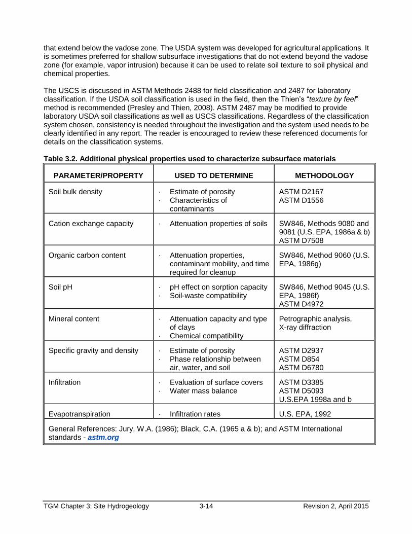
that extend below the vadose zone. The USDA system was developed for agricultural applications. It is sometimes preferred for shallow subsurface investigations that do not extend beyond the vadose zone (for example, vapor intrusion) because it can be used to relate soil texture to soil physical and chemical properties. The USCS is discussed in ASTM Methods 2488 for field classification and 2487 for laboratory classification. If the USDA soil classification is used in the field, then the Thien’s “texture by feel” method is recommended (Presley and Thien, 2008). ASTM 2487 may be modified to provide laboratory USDA soil classifications as well as USCS classifications. Regardless of the classification system chosen, consistency is needed throughout the investigation and the system used needs to be clearly identified in any report. The reader is encouraged to review these referenced documents for details on the classification systems. Table 3.2. Additional physical properties used to characterize subsurface materials

PARAMETER/PROPERTY

USED TO DETERMINE

METHODOLOGY

Soil bulk density

· Estimate of porosity · Characteristics of

contaminants

ASTM D2167 ASTM D1556

Cation exchange capacity

· Attenuation properties of soils

SW846, Methods 9080 and 9081 (U.S. EPA, 1986a & b) ASTM D7508

Organic carbon content

· Attenuation properties,

contaminant mobility, and time required for cleanup

SW846, Method 9060 (U.S. EPA, 1986g)

Soil pH

· pH effect on sorption capacity · Soil-waste compatibility

SW846, Method 9045 (U.S. EPA, 1986f) ASTM D4972

Mineral content

· Attenuation capacity and type

of clays · Chemical compatibility

Petrographic analysis, X-ray diffraction

Specific gravity and density

· Estimate of porosity · Phase relationship between

air, water, and soil

ASTM D2937 ASTM D854 ASTM D6780

Infiltration

· Evaluation of surface covers · Water mass balance

ASTM D3385 ASTM D5093 U.S.EPA 1998a and b

Evapotranspiration

· Infiltration rates

U.S. EPA, 1992

General References: Jury, W.A. (1986); Black, C.A. (1965 a & b); and ASTM International standards - astm.org

TGM Chapter 3: Site Hydrogeology 3-15 Revision 2, April 2015

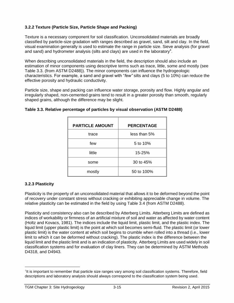
3.2.2 Texture (Particle Size, Particle Shape and Packing) Texture is a necessary component for soil classification. Unconsolidated materials are broadly classified by particle-size gradation with ranges described as gravel, sand, silt and clay. In the field, visual examination generally is used to estimate the range in particle size. Sieve analysis (for gravel and sand) and hydrometer analysis (silts and clays) are used in the laboratory4. When describing unconsolidated materials in the field, the description should also include an estimation of minor components using descriptive terms such as trace, little, some and mostly (see Table 3.3. (from ASTM D2488)). The minor components can influence the hydrogeologic characteristics. For example, a sand and gravel with “few” silts and clays (5 to 10%) can reduce the effective porosity and hydraulic conductivity. Particle size, shape and packing can influence water storage, porosity and flow. Highly angular and irregularly shaped, non-cemented grains tend to result in a greater porosity than smooth, regularly shaped grains, although the difference may be slight. Table 3.3. Relative percentage of particles by visual observation (ASTM D2488)

PARTICLE AMOUNT

PERCENTAGE

trace less than 5%

few 5 to 10%

little 15-25%

some 30 to 45%

mostly 50 to 100%

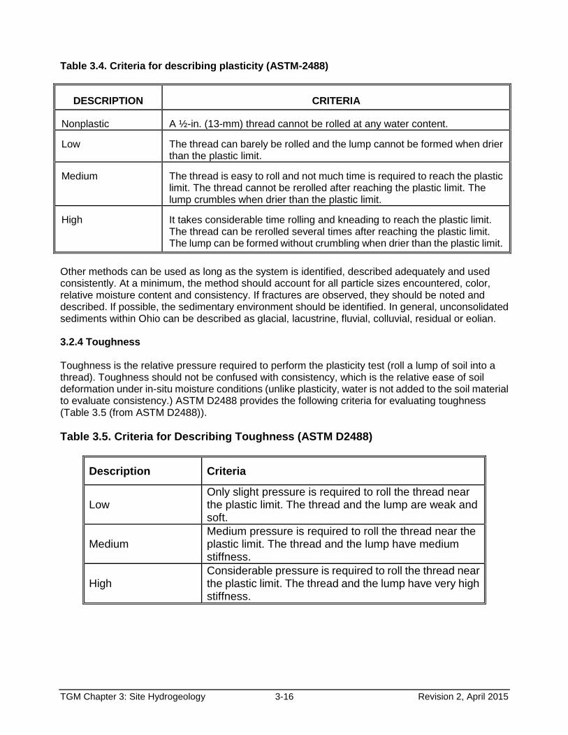
3.2.3 Plasticity Plasticity is the property of an unconsolidated material that allows it to be deformed beyond the point of recovery under constant stress without cracking or exhibiting appreciable change in volume. The relative plasticity can be estimated in the field by using Table 3.4 (from ASTM D2488). Plasticity and consistency also can be described by Atterberg Limits. Atterberg Limits are defined as indices of workability or firmness of an artificial mixture of soil and water as affected by water content (Holtz and Kovacs, 1981). The indices include the liquid limit, plastic limit, and the plastic index. The liquid limit (upper plastic limit) is the point at which soil becomes semi-fluid. The plastic limit (or lower plastic limit) is the water content at which soil begins to crumble when rolled into a thread (i.e., lower limit to which it can be deformed without cracking). The plastic index is the difference between the liquid limit and the plastic limit and is an indication of plasticity. Atterberg Limits are used widely in soil classification systems and for evaluation of clay liners. They can be determined by ASTM Methods D4318, and D4943.

4It is important to remember that particle size ranges vary among soil classification systems. Therefore, field

descriptions and laboratory analysis should always correspond to the classification system being used.

TGM Chapter 3: Site Hydrogeology 3-16 Revision 2, April 2015

Table 3.4. Criteria for describing plasticity (ASTM-2488) DESCRIPTION

CRITERIA

Nonplastic

A ½-in. (13-mm) thread cannot be rolled at any water content.

Low

The thread can barely be rolled and the lump cannot be formed when drier than the plastic limit.

Medium

The thread is easy to roll and not much time is required to reach the plastic limit. The thread cannot be rerolled after reaching the plastic limit. The lump crumbles when drier than the plastic limit.

High

It takes considerable time rolling and kneading to reach the plastic limit. The thread can be rerolled several times after reaching the plastic limit. The lump can be formed without crumbling when drier than the plastic limit.

Other methods can be used as long as the system is identified, described adequately and used consistently. At a minimum, the method should account for all particle sizes encountered, color, relative moisture content and consistency. If fractures are observed, they should be noted and described. If possible, the sedimentary environment should be identified. In general, unconsolidated sediments within Ohio can be described as glacial, lacustrine, fluvial, colluvial, residual or eolian. 3.2.4 Toughness Toughness is the relative pressure required to perform the plasticity test (roll a lump of soil into a thread). Toughness should not be confused with consistency, which is the relative ease of soil deformation under in-situ moisture conditions (unlike plasticity, water is not added to the soil material to evaluate consistency.) ASTM D2488 provides the following criteria for evaluating toughness (Table 3.5 (from ASTM D2488)).

Table 3.5. Criteria for Describing Toughness (ASTM D2488)

Description Criteria

Low Only slight pressure is required to roll the thread near the plastic limit. The thread and the lump are weak and soft.

Medium Medium pressure is required to roll the thread near the plastic limit. The thread and the lump have medium stiffness.

High Considerable pressure is required to roll the thread near the plastic limit. The thread and the lump have very high stiffness.

TGM Chapter 3: Site Hydrogeology 3-17 Revision 2, April 2015

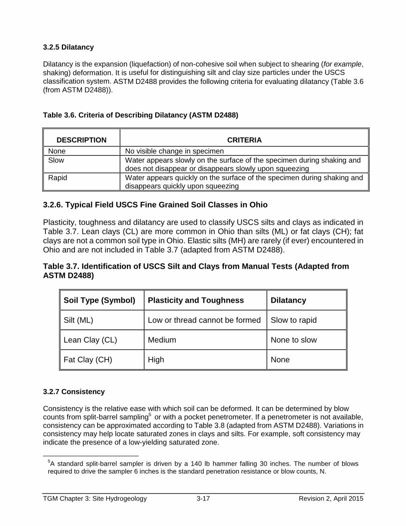
3.2.5 Dilatancy Dilatancy is the expansion (liquefaction) of non-cohesive soil when subject to shearing (for example,

shaking) deformation. It is useful for distinguishing silt and clay size particles under the USCS

classification system. ASTM D2488 provides the following criteria for evaluating dilatancy (Table 3.6 (from ASTM D2488)). Table 3.6. Criteria of Describing Dilatancy (ASTM D2488)

DESCRIPTION

CRITERIA

None No visible change in specimen

Slow Water appears slowly on the surface of the specimen during shaking and does not disappear or disappears slowly upon squeezing

Rapid Water appears quickly on the surface of the specimen during shaking and disappears quickly upon squeezing

3.2.6. Typical Field USCS Fine Grained Soil Classes in Ohio

Plasticity, toughness and dilatancy are used to classify USCS silts and clays as indicated in Table 3.7. Lean clays (CL) are more common in Ohio than silts (ML) or fat clays (CH); fat clays are not a common soil type in Ohio. Elastic silts (MH) are rarely (if ever) encountered in Ohio and are not included in Table 3.7 (adapted from ASTM D2488).

Table 3.7. Identification of USCS Silt and Clays from Manual Tests (Adapted from ASTM D2488)

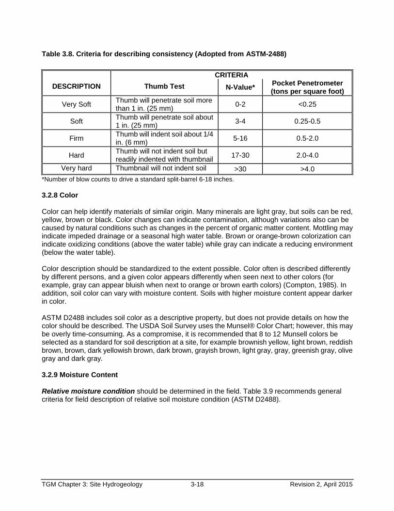
3.2.7 Consistency Consistency is the relative ease with which soil can be deformed. It can be determined by blow counts from split-barrel sampling5 or with a pocket penetrometer. If a penetrometer is not available, consistency can be approximated according to Table 3.8 (adapted from ASTM D2488). Variations in consistency may help locate saturated zones in clays and silts. For example, soft consistency may indicate the presence of a low-yielding saturated zone.

5A standard split-barrel sampler is driven by a 140 lb hammer falling 30 inches. The number of blows

required to drive the sampler 6 inches is the standard penetration resistance or blow counts, N.

Soil Type (Symbol) Plasticity and Toughness Dilatancy

Silt (ML) Low or thread cannot be formed Slow to rapid

Lean Clay (CL) Medium None to slow

Fat Clay (CH) High None

TGM Chapter 3: Site Hydrogeology 3-18 Revision 2, April 2015

Table 3.8. Criteria for describing consistency (Adopted from ASTM-2488)

*Number of blow counts to drive a standard split-barrel 6-18 inches.

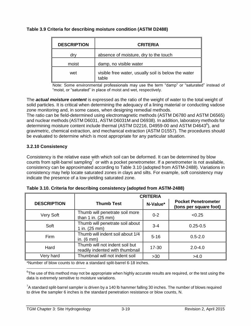
3.2.8 Color Color can help identify materials of similar origin. Many minerals are light gray, but soils can be red, yellow, brown or black. Color changes can indicate contamination, although variations also can be caused by natural conditions such as changes in the percent of organic matter content. Mottling may indicate impeded drainage or a seasonal high water table. Brown or orange-brown colorization can indicate oxidizing conditions (above the water table) while gray can indicate a reducing environment (below the water table). Color description should be standardized to the extent possible. Color often is described differently by different persons, and a given color appears differently when seen next to other colors (for example, gray can appear bluish when next to orange or brown earth colors) (Compton, 1985). In addition, soil color can vary with moisture content. Soils with higher moisture content appear darker in color. ASTM D2488 includes soil color as a descriptive property, but does not provide details on how the color should be described. The USDA Soil Survey uses the Munsel® Color Chart; however, this may be overly time-consuming. As a compromise, it is recommended that 8 to 12 Munsell colors be selected as a standard for soil description at a site, for example brownish yellow, light brown, reddish brown, brown, dark yellowish brown, dark brown, grayish brown, light gray, gray, greenish gray, olive gray and dark gray. 3.2.9 Moisture Content Relative moisture condition should be determined in the field. Table 3.9 recommends general criteria for field description of relative soil moisture condition (ASTM D2488).

CRITERIA

DESCRIPTION Thumb Test N-Value* Pocket Penetrometer (tons per square foot)

Very Soft Thumb will penetrate soil more than 1 in. (25 mm)

0-2 <0.25

Soft Thumb will penetrate soil about 1 in. (25 mm)

3-4 0.25-0.5

Firm Thumb will indent soil about 1/4 in. (6 mm)

5-16 0.5-2.0

Hard Thumb will not indent soil but readily indented with thumbnail

17-30 2.0-4.0

Very hard Thumbnail will not indent soil >30 >4.0

TGM Chapter 3: Site Hydrogeology 3-19 Revision 2, April 2015

Table 3.9 Criteria for describing moisture condition (ASTM D2488)

DESCRIPTION

CRITERIA

dry

absence of moisture, dry to the touch

moist

damp, no visible water

wet

visible free water, usually soil is below the water table

Note: Some environmental professionals may use the term “damp” or “saturated” instead of “moist, or “saturated” in place of moist and wet, respectively.

The actual moisture content is expressed as the ratio of the weight of water to the total weight of solid particles. It is critical when determining the adequacy of a lining material or conducting vadose zone monitoring and, in some cases, when designing remedial methods. The ratio can be field-determined using electromagnetic methods (ASTM D6780 and ASTM D6565) and nuclear methods (ASTM D6031, ASTM D6031M and D6938). In addition, laboratory methods for determining moisture content include thermal (ASTM D2216, D4959-00 and ASTM D46436), and gravimetric, chemical extraction, and mechanical extraction (ASTM D1557). The procedures should be evaluated to determine which is most appropriate for any particular situation. 3.2.10 Consistency Consistency is the relative ease with which soil can be deformed. It can be determined by blow counts from split-barrel sampling7 or with a pocket penetrometer. If a penetrometer is not available, consistency can be approximated according to Table 3.10 (adopted from ASTM-2488). Variations in consistency may help locate saturated zones in clays and silts. For example, soft consistency may indicate the presence of a low-yielding saturated zone. Table 3.10. Criteria for describing consistency (adopted from ASTM-2488)

*Number of blow counts to drive a standard split-barrel 6-18 inches.

6The use of this method may not be appropriate when highly accurate results are required, or the test using the

data is extremely sensitive to moisture variations. 7A standard split-barrel sampler is driven by a 140 lb hammer falling 30 inches. The number of blows required

to drive the sampler 6 inches is the standard penetration resistance or blow counts, N.

CRITERIA

DESCRIPTION Thumb Test N-Value* Pocket Penetrometer (tons per square foot)

Very Soft Thumb will penetrate soil more than 1 in. (25 mm)

0-2 <0.25

Soft Thumb will penetrate soil about 1 in. (25 mm)

3-4 0.25-0.5

Firm Thumb will indent soil about 1/4 in. (6 mm)

5-16 0.5-2.0

Hard Thumb will not indent soil but readily indented with thumbnail

17-30 2.0-4.0

Very hard Thumbnail will not indent soil >30 >4.0

TGM Chapter 3: Site Hydrogeology 3-20 Revision 2, April 2015

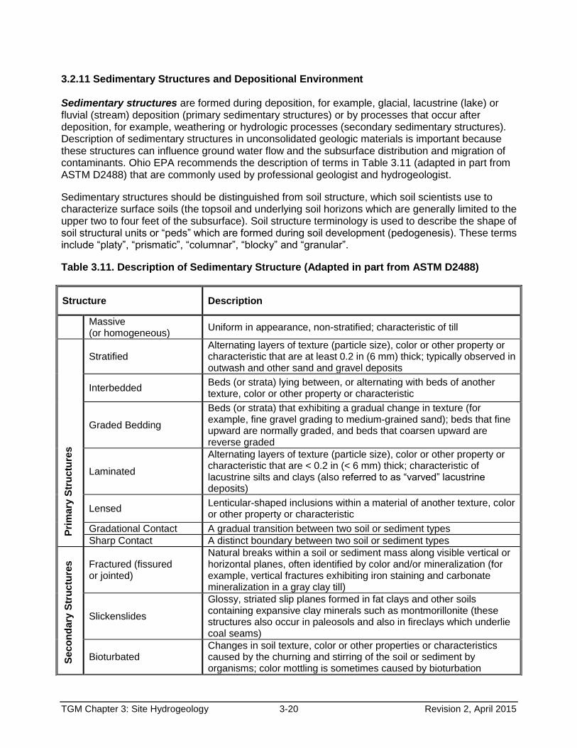
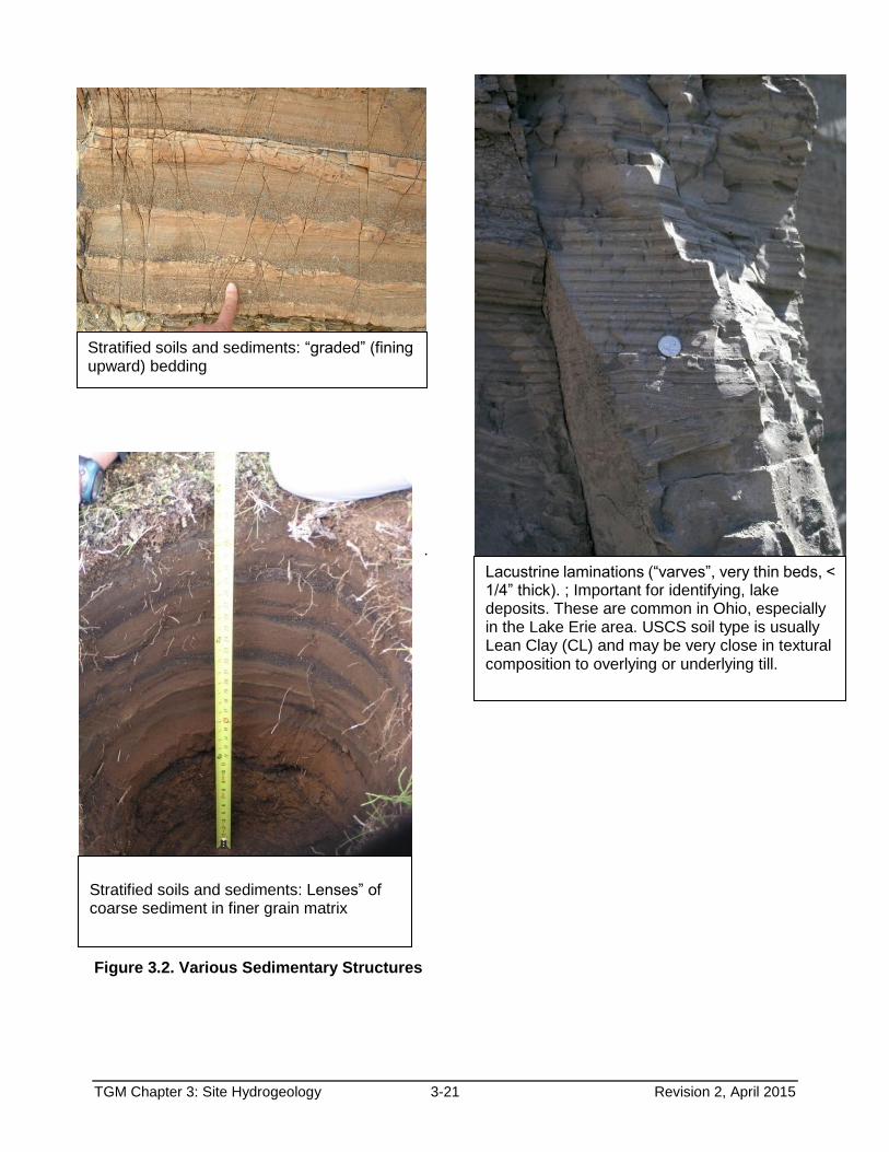
3.2.11 Sedimentary Structures and Depositional Environment Sedimentary structures are formed during deposition, for example, glacial, lacustrine (lake) or fluvial (stream) deposition (primary sedimentary structures) or by processes that occur after deposition, for example, weathering or hydrologic processes (secondary sedimentary structures). Description of sedimentary structures in unconsolidated geologic materials is important because these structures can influence ground water flow and the subsurface distribution and migration of contaminants. Ohio EPA recommends the description of terms in Table 3.11 (adapted in part from ASTM D2488) that are commonly used by professional geologist and hydrogeologist.

Sedimentary structures should be distinguished from soil structure, which soil scientists use to characterize surface soils (the topsoil and underlying soil horizons which are generally limited to the upper two to four feet of the subsurface). Soil structure terminology is used to describe the shape of soil structural units or “peds” which are formed during soil development (pedogenesis). These terms include “platy”, “prismatic”, “columnar”, “blocky” and “granular”.

Table 3.11. Description of Sedimentary Structure (Adapted in part from ASTM D2488)

Structure Description

Massive (or homogeneous)

Uniform in appearance, non-stratified; characteristic of till

P

rim

ary

Str

uc

ture

s

Stratified Alternating layers of texture (particle size), color or other property or characteristic that are at least 0.2 in (6 mm) thick; typically observed in outwash and other sand and gravel deposits

Interbedded Beds (or strata) lying between, or alternating with beds of another texture, color or other property or characteristic

Graded Bedding

Beds (or strata) that exhibiting a gradual change in texture (for example, fine gravel grading to medium-grained sand); beds that fine upward are normally graded, and beds that coarsen upward are reverse graded

Laminated

Alternating layers of texture (particle size), color or other property or characteristic that are < 0.2 in (< 6 mm) thick; characteristic of lacustrine silts and clays (also referred to as “varved” lacustrine deposits)

Lensed Lenticular-shaped inclusions within a material of another texture, color or other property or characteristic

Gradational Contact A gradual transition between two soil or sediment types

Sharp Contact A distinct boundary between two soil or sediment types

S

eco

nd

ary

Str

uc

ture

s

Fractured (fissured or jointed)

Natural breaks within a soil or sediment mass along visible vertical or horizontal planes, often identified by color and/or mineralization (for example, vertical fractures exhibiting iron staining and carbonate mineralization in a gray clay till)

Slickenslides

Glossy, striated slip planes formed in fat clays and other soils containing expansive clay minerals such as montmorillonite (these structures also occur in paleosols and also in fireclays which underlie coal seams)

Bioturbated Changes in soil texture, color or other properties or characteristics caused by the churning and stirring of the soil or sediment by organisms; color mottling is sometimes caused by bioturbation

TGM Chapter 3: Site Hydrogeology 3-21 Revision 2, April 2015

.

Figure 3.2. Various Sedimentary Structures

Stratified soils and sediments: Lenses” of coarse sediment in finer grain matrix

Stratified soils and sediments: “graded” (fining upward) bedding

Lacustrine laminations (“varves”, very thin beds, < 1/4” thick). ; Important for identifying, lake deposits. These are common in Ohio, especially in the Lake Erie area. USCS soil type is usually Lean Clay (CL) and may be very close in textural composition to overlying or underlying till.

TGM Chapter 3: Site Hydrogeology 3-22 Revision 2, April 2015

Depositional environment describes the combination of physical, chemical and biological processes associated with the deposition of a particular sediment type. Depositional environments are identified based on the geologic interpretation of texture, sedimentary structures and other sediment characteristics. Identification of depositional environments is helpful for development of site conceptual models (especially at large sites or properties) because knowledge of depositional environment can help to correlate or interpolate subsurface conditions between boring locations and to predict the most likely contaminant migration pathways.

Much of Ohio is underlain by glacial till, and the term “till” is sometimes used on boring logs as a soil type classification, generally as a synonym for clay or silty clay. This is improper because “till” does not refer to soil type but to the specific depositional environment, i.e., non-texture specific, non-stratified sediment that is deposited under a glacier without subsequent reworking (Jackson, J.A., 1997). If the soil type is a silt or clay it should be classified as such, for example, “lean clay”, “silty clay loam”, etc., and its depositional environment identified as “till” if it exhibits the appropriate characteristics.

3.3 DESCRIPTION AND CLASSIFICATION OF CONSOLIDATED MATERIALS The uppermost consolidated units (bedrock) in Ohio are sedimentary and generally consist of carbonate rock, sandstone, shale or coal that ranges in age from Ordovician to Permian. Distinctive characteristics that are influential with respect to ground water movement include porosity, permeability, fracturing (including stress release), bedding and solution weathering (karst). Porosity and hydraulic conductivity measurements are discussed later in this chapter. Fractures can be identified by a boring program and fracture trace analysis. Bedding plane spacing, strike, and dip should be indicated. Prominent bedding planes should be distinguished from banding due to color or textural variation. An attempt should be made to determine the formation name to assess regional characteristics. The competence of the consolidated materials can be described by the Rock Quality Designation (RQD). The RQD is calculated by measuring the total length of all competent core pieces greater than four or more inches, dividing it by the length of the core run, and multiplying by 100. Competent core sections are those that do not exhibit natural fracturing but may have been fractured during the drilling process (See Section 3.4: Fracturing).

In general, the higher the RQD value, the higher the integrity of the rock. Table 3.12 lists RQD and a description of rock quality (Ruda et al., 2006).

Table 3.12. Correlation Between RQD and Rock Mass Quality (Ruda et al., 2006)

RQD

Description of Rock Quality

0-25

Very Poor

50

Poor

75

Fair

90

Good

100

Excellent

TGM Chapter 3: Site Hydrogeology 3-23 Revision 2, April 2015

3.4 FRACTURING Fractures are breaks in geologic material due to stress. As they play an important role in the movement of water and contaminants through bedrock and unconsolidated materials, their presence needs to be identified and evaluated. However, the mere presence of fractures may not be enough to allow for ground water flow. Aspects of fractures that may need to be evaluated to determine if the fractures contribute or control ground water flow include orientation, density, depth, aperture opening and connectivity. Clayey soils are generally assumed to act as low permeability confining units, providing acceptable isolation distances to underlying ground water resources that could be impacted by contaminant sources. However, if fractures and other macropores are not adequately evaluated and accounted for, the hydraulic conductivity of clayey soils may be underestimated by as much as two to four orders of magnitude. Consolidated rocks can contain secondary porosity and permeability due to fracturing. Microfractures in bedrock may add very little to the original hydraulic conductivity; however, major fracture zones may have localized hydraulic conductivities several orders of magnitude greater than that of the unfractured rock (Fetter, 2001). Fractures can be highly localized and unpredictable or more evenly distributed (Nielsen et al., 2006). Accordingly, the evaluation of fractures is critical for the proper siting, design and operation of waste disposal units; evaluation of the potential for existing contaminant sources to affect the ground water; interpretation of ground water flow; and the fate and transport of contaminants. It should be noted that fractures can be induced from drilling and coring. It can be difficult to distinguish between natural and induced occurrences. However, distinguishing between naturally-occurring fractures and coring-induced fractures is very important. Natural fractures often occur at high (near-vertical) or low (near-horizontal) angles and exhibit oxidation, weathering and/or mineralization along their surfaces as opposed to coring-induced fractures which do not. Coring–induced fractures typically are formed at angles of 30 to 60 degrees in massive sedimentary rocks such as sandstone or crystalline limestone and along horizontal bedding planes in highly stratified or laminated rocks such as shale or siltstone. Bedding plane fractures also may be formed in core (especially shale) due to vertical expansion in response to the relief of overburden pressure. However, the absence of those features does not necessarily imply inducement. Information concerning natural versus induced fractures in rock cores has been provided by Kulander et al. (1990). Methods to help determine the presence or absence of fractures and/or their effects on the flow characteristics of fractured media include subsurface sampling and description; environmental isotopes; tracer tests; hydraulic tests; water level measurements; major ion and indicator parameters; logging/flow meters; and fracture trace analysis. Subsurface sampling when boring/coring and observation while trenching can be used to identify fractures. Angled borings may be helpful in locating vertical fractures. Due to cost, safety, and logistics, angled borings are not generally completed. However, angled boring is a promising technology whose application is evolving (Kinner et al, 2005). In some areas, road cuts, excavations and outcrops can provide reliable and easy access to gather data on fractures in bedrock formations. Trenching is particularly useful when evaluating near-surface conditions in both unconsolidated material and shallow bedrock. In bedrock, to maintain the maximal benefit from trenches, they should be perpendicular to the strike of the lithological sequences, alteration zones, or major structural discontinuities (Sara, 2003). Trenches can be excavated to approximately 15 feet. Worker health

TGM Chapter 3: Site Hydrogeology 3-24 Revision 2, April 2015

and safety should be carefully considered during any trenching operation. Safety plans may be necessary when trenching. The presence and relative prevalence of fractures or other macropores should be noted. Fractures should be described with respect to orientation (i.e., vertical versus horizontal), approximate spacing, and, if possible, approximate width. Fracture surfaces should be inspected for open space, mineralization, and the presence of ground water. Any apparent associations between the occurrence of fractures and variation in other subsurface characteristics, for example, alteration, color, texture, moisture content, consistency or plasticity, stratification, etc., should be recorded. Documentation of color changes is important. For example, weathered and fractured clayey soils tend to be brown (due to the oxidation of Fe+2 to Fe+3) as opposed to relatively unweathered and unfractured clayey soils, which tend to be gray. Fractures facilitate weathering and oxidation within the subsurface, and color variation may be used to estimate the depth of hydraulically-active fractures at some localities. Any transitional zones of color change should be noted, as well as any color “halos” associated with fractures that extend into apparently unweathered clayey soils. These features often indicate the presence of hydraulically-active fractures. Any secondary mineralization or alteration observed within fractures should be documented. A high degree of mineralization suggests that fractures may not be hydraulically active. Furthermore, observing mineralization (for example, authigenic gypsum) may aid in understanding the spatial variability of recharge through fracture-related flow regimes (Keller et al., 1991). Filling of fracture surfaces can control the rate and direction of ground water flow. Fracture filling can be affected by waste leachate that may have the potential to remove portions of the fracture blockage (Sara, 2003). Environmental isotopes and isotopic age-dating to estimate the age of the water in unconsolidated sediments may be useful in evaluating the flow of ground water through clayey confining layers. This may be helpful in determining whether fractures, if present, are transmitting water. With respect to evaluating ground water flow through fractured clayey soils, 3H (tritium) and O18 are particularly useful in demonstrating the effective depth of fracture flow systems in clayey soils as well as providing ground water velocity and age estimates (Gerber and Howard, 2000; Simpkins and Bradbury, 1992; Rudolph et al., 1991; Ruland et al., 1991; D’Astous et al., 1989; Hendry, 1988; Keller et al., 1988 and 1986; Barari and Hedges, 1985; and Bradbury et al., 1985.) Ground water tracer tests can be designed to estimate the hydraulic conductivity of fractured media, and can also provide estimates of fracture aperture, effective fracture porosity, and fracture flow velocity. A chemical tracer (sodium bromide) investigation by D’Astous et al. (1989) in fractured Wisconsinan-age clayey till underlying the Sarnia area of southwestern Ontario provided hydraulic conductivity estimates that corresponded well with the results of a recovery test from a large-diameter well completed in the same zone. Hydraulic tests (for example, pumping and slug tests)8 may be helpful in determining whether fractures occurring in clays are transmitting fluid. Hydraulic testing methods evaluate a much larger portion of the clayey soil unit compared to laboratory tests, and therefore are more sensitive to fracture-related hydraulic conductivity.

Single well pumping tests are not recommended for estimating hydraulic conductivity in fractured clayey soils because of the difficulty of obtaining a constant pumping rate and the potential complications involving well loss and well storage.

8Slug and Pumping Tests is discussed in more detail in TGM Chapter 4.

TGM Chapter 3: Site Hydrogeology 3-25 Revision 2, April 2015

Slug tests are acceptable for evaluating hydraulic conductivity of fractured clayey soils, provided that the monitoring well or piezometer is properly constructed and developed, and that the boring walls have not been badly smeared or deformed during the drilling process (Döll and Schneider, 1995; Jones, 1993; Bradbury and Muldoon, 1990; D’Astous et al., 1989; Keller et al., 1989; Keller et al., 1986). The number of slug tests necessary to provide a representative estimate of hydraulic conductivity for a given saturated unit depends on site-specific conditions. Based on the studies reviewed, the Hvorslev (1951) analytical method appears to be favored for estimation of hydraulic conductivity for clayey tills (Bruner and Lutenegger, 1993; Jones 1993; Simpkins and Bradbury, 1992; Rudolph et al., 1991; Ruland et al., 1991; D’Astous et al., 1989; Keller et al., 1989; Hendry, 1988; Cravens and Ruedisili, 1987; Keller et al., 1986; Bradbury et al., 1985; Prudic, 1982). However, this method should not be used for clayey soils that are highly compressible (for example, soft, saturated lacustrine silt and clay) as neglecting the storage capacity of such a medium could result in a large error (Döll and Schneider, 1995).

Multiple well pumping tests provide a better estimate of hydraulic conductivity because they are performed on a larger scale. They can better establish the spatial extent of fracture flow in clay (Jones, 1993; Strobel, 1993; Hendry, 1988; Keller et al., 1986). However, performing a pumping test in saturated clay soils is technically challenging.

In fractured bedrock, packer hydraulic conductivity tests should be considered. Intervals identified during the coring program should be selected for packer intervals to test specific, observed discontinuities (Nieslen et al., 2006). Water level monitoring on a weekly to monthly basis can help establish the maximum depth of fracture flow in clayey soils (Ruland et al., 1991; D’Astous et al., 1989), as well as help evaluate the effectiveness of clayey soil units in protecting underlying ground water resources (Baehr and Turley, 2000; Keller et al., 1988). Near-surface, heavily fractured clayey soils tend to exhibit greater water level fluctuations in response to changes in precipitation and evapotranspiration conditions than do underlying, relatively unfractured clayey soils or underlying confined saturated units (Baehr and Turley, 2000; Rudolph et al., 1991; Ruland et al., 1991; D’Astous et al., 1989; Keller et al., 1989; Hendry, 1988; Keller et al., 1988; Barari and Hedges, 1985; Hendry, 1982). Additionally, fractured clayey soils more frequently exhibit lower or upward hydraulic gradients due to discharge through evapotranspiration (Simpkins and Bradbury, 1992; Ruland et al., 1991; D’Astous et al., 1989; Hendry, 1988; Cravens and Ruedisili, 1987; Barari and Hedges, 1985). Ruland et al. (1991) and Cravens and Ruedisili (1987) attribute the larger variance of hydraulic gradients in unweathered tills to greater grain-size sensitivity, as unweathered tills generally contain fewer fractures and other macropores compared to weathered tills. Major-ion and indicator parameter geochemistry of ground water samples from clayey soils can be used to evaluate the effective depth of fracture-related flow. Comparison of major-ion concentrations, as well as total dissolved solids and specific conductance, in ground water from weathered, fractured clayey soils and ground water from unweathered, relatively unfractured clayey soils by Cravens and Ruedisili (1987), Hendry et al. (1986), Barari and Hedges (1985), and Bradbury et al. (1985) shows that concentrations of Ca+2, Mg+2, K+, Na+, SO4

-2, TDS, and/or specific conductance tend to be higher in weathered, fractured clayey soils, and Cl- concentrations tend to be higher in underlying unweathered clayey soils. The approximate depths at which changes in these concentrations occurred corresponded with changes in hydraulic conductivity or hydraulic head data indicative of a transition from fractured to relatively unfractured environments. Cravens and Ruedisili (1987) concluded that low major-ion concentrations in ground water from the Tulare sand-and-gravel

TGM Chapter 3: Site Hydrogeology 3-26 Revision 2, April 2015

aquifer in Hyde and Hand Counties, South Dakota, indicate low recharge rates from the overlying unweathered till layer, which contains ground water with significantly higher major-ion concentrations. Geophysical tools can also be used to help identify fractures. A suite of borehole geophysical tools (for example, temperature and conductivity logs, natural gamma and caliper logs, borehole radar, tomography, optical and acoustic televiewer) are commonly being used in fractured rock. Borehole flow meters also appear to be useful for evaluating fractures in bedrock (Kinner et al., 2005). Borehole imaging and flow meter logging provide a means for evaluating fracture frequency and orientations and isolating hydraulically conductive fracture systems. McKay et al. (1998) discuss a case study of use of a borehole flow meter. Recent borehole flow meter surveys at the Oak Ridge Reservation in Tennessee (Will, et al., 1992 in U.S. EPA, 1993) illustrate some of the problems encountered in fractured media. Based on drilling records, core samples and geophysical/downhole camera surveys of a 405 foot deep borehole, CH-9, it appeared that the shales at this site were highly fractured with typical fracture spacings of a few inches to a few feet. However, an electromagnetic flow meter survey under ambient conditions (no pumping) indicated that flow was restricted to two narrow zones at 135 and 330 foot depths. Flow was found to enter the deeper zone, then flow up the well bore and exit into the shallow fracture zone with a flow rate of up to 0.2 gallons per minute (gpm) or about 700 gal per day (gpd). This presents several potential problems, primarily the possible mixing of contaminated and uncontaminated waters. Fracture trace analysis can help locate fractures. Fracture traces are surface expressions of joints or faults. Many of the linear features detected on aerial photos or imagery are surface expressions of fractures in bedrock more than 100 feet deep (Nielsen et al., 2006). On aerial photos, natural linear features appear as tonal variation in soils, alignment of vegetative patterns, straight stream segments or valleys, alignment of surface depressions, gaps in ridges, or other features showing linear orientation that may be related to fractures (Fetter, 2001). Valley and stream segments tend to run along fractures and joints because these zones are more susceptible to erosion. Alignment of sinkholes are typical surface expressions in areas of carbonate bedrock. Other features that show linear orientation, such as swales, gullies, or sags, form due to soil settling into fractures or fault zones (Nielsen et al., 2006). 3.5 ANTHROPOGENIC INFLUENCE Man-made activities and structures such as fill material, utility lines, and ground water pumping can influence the direction of ground water flow and create pathways for contaminant migration. Their presence and influence at a site need to be understood.

Anthropogenic (human-related) influences on soils and other unconsolidated geologic materials include excavation and movement of in-situ or native material and the addition of non-native materials, including wastes. Waste materials may include solids (for example, municipal solid wastes, industrial or residual solid wastes, foundry sand, slag, cinders, construction and demolition debris, concrete or asphalt) or liquids (for example, petroleum products, solvents or sewage). When describing soils for hydrogeologic investigations associated with environmental assessments, both of these influences are critical to document for the evaluation of ground water movement and the distribution and migration of contaminants. Identification of soil fill is sometimes difficult, especially if the fill is similar in composition or origin to in-situ soils. However, distinguishing fill from in-situ material is important. Even if the fill material

TGM Chapter 3: Site Hydrogeology 3-27 Revision 2, April 2015

originated from another soil unit on the same site, the hydrogeologic properties of the fill (for example, bulk density, porosity, hydraulic conductivity, etc.) material are very likely different than that of the parent material due to the disturbance associated with the excavation and movement of the material. Typically, the presence of solid wastes or debris such as broken glass, slag or concrete fragments provides evidence that subsurface material has been distributed. The impacts of regional and local withdrawal of water can influence the direction of ground water flow. Pumping wells can alter the flow direction or can cause interconnection between ground water zones. Underground utility lines running through the property may influence the migration of water and contaminants. They need to be assessed to ensure protection of human health and the environment. 3.6 GROUND WATER OCCURRENCE The subsurface can be classified into unsaturated (vadose) and saturated (phreatic) zones. In the unsaturated zone, both water and air occur in the pores. In the saturated zone, the pores are filled with water. The intent of this section is to explain the minimum characteristics necessary to characterize saturated zones that contain ground water that will enhance ground water movement. Direct techniques to characterize ground water occurrence, such as installation of monitoring wells and piezometers, are generally necessary. Additional information can be found in Fetter (2001), Todd (2001), and Freeze and Cherry (1979). Regulatory requirements may dictate the nature of the investigation for facility siting and ground water monitoring. For example, some regulations, such as those governing solid waste landfills, mandate that an owner/operator define an “uppermost aquifer system” and demonstrate that it is protected adequately before a landfill can be permitted. Additionally, these regulations specify that significant saturated zones above the uppermost aquifer system must be identified and monitored. Ground water in the saturated zone can occur under confined or unconfined conditions. A confined zone is bounded by relatively impermeable layers. Water levels in wells completed in a confined zone rise above the base of an upper confining layer. These levels define an imaginary surface called the potentiometric or piezometric surface. A zone that has a water table as its upper boundary is termed unconfined. "Water table" is defined as a surface where hydrostatic pressure equals atmospheric pressure. In general, most water-bearing zones are not entirely confined or unconfined and often are referred to as leaky or semi-confined. Identifying confining conditions is important in selecting the appropriate hydraulic test for determining hydraulic conductivity and predicting ground water vulnerability. Unconfined zones are at greater risk of contamination from surface activities than confined zones. A special case of an unconfined zone is a perched water table, which may develop when a relatively impervious layer of limited horizontal area (for example, clay lens) is located between the water table and the ground surface. Ground water accumulates above this impervious layer. Perched zones may drain into an underlying zone or may be permanent. Permanent zones may serve as a supply of drinking water.

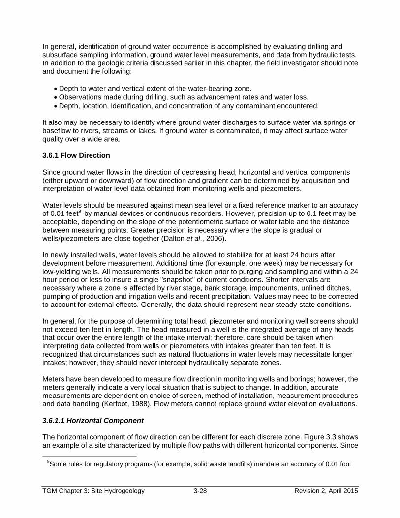
TGM Chapter 3: Site Hydrogeology 3-28 Revision 2, April 2015

In general, identification of ground water occurrence is accomplished by evaluating drilling and subsurface sampling information, ground water level measurements, and data from hydraulic tests. In addition to the geologic criteria discussed earlier in this chapter, the field investigator should note and document the following:

Depth to water and vertical extent of the water-bearing zone.

Observations made during drilling, such as advancement rates and water loss.

Depth, location, identification, and concentration of any contaminant encountered.

It also may be necessary to identify where ground water discharges to surface water via springs or baseflow to rivers, streams or lakes. If ground water is contaminated, it may affect surface water quality over a wide area. 3.6.1 Flow Direction Since ground water flows in the direction of decreasing head, horizontal and vertical components (either upward or downward) of flow direction and gradient can be determined by acquisition and interpretation of water level data obtained from monitoring wells and piezometers. Water levels should be measured against mean sea level or a fixed reference marker to an accuracy of 0.01 feet9 by manual devices or continuous recorders. However, precision up to 0.1 feet may be acceptable, depending on the slope of the potentiometric surface or water table and the distance between measuring points. Greater precision is necessary where the slope is gradual or wells/piezometers are close together (Dalton et al., 2006). In newly installed wells, water levels should be allowed to stabilize for at least 24 hours after development before measurement. Additional time (for example, one week) may be necessary for low-yielding wells. All measurements should be taken prior to purging and sampling and within a 24 hour period or less to insure a single "snapshot" of current conditions. Shorter intervals are necessary where a zone is affected by river stage, bank storage, impoundments, unlined ditches, pumping of production and irrigation wells and recent precipitation. Values may need to be corrected to account for external effects. Generally, the data should represent near steady-state conditions. In general, for the purpose of determining total head, piezometer and monitoring well screens should not exceed ten feet in length. The head measured in a well is the integrated average of any heads that occur over the entire length of the intake interval; therefore, care should be taken when interpreting data collected from wells or piezometers with intakes greater than ten feet. It is recognized that circumstances such as natural fluctuations in water levels may necessitate longer intakes; however, they should never intercept hydraulically separate zones. Meters have been developed to measure flow direction in monitoring wells and borings; however, the meters generally indicate a very local situation that is subject to change. In addition, accurate measurements are dependent on choice of screen, method of installation, measurement procedures and data handling (Kerfoot, 1988). Flow meters cannot replace ground water elevation evaluations. 3.6.1.1 Horizontal Component The horizontal component of flow direction can be different for each discrete zone. Figure 3.3 shows an example of a site characterized by multiple flow paths with different horizontal components. Since

9Some rules for regulatory programs (for example, solid waste landfills) mandate an accuracy of 0.01 foot

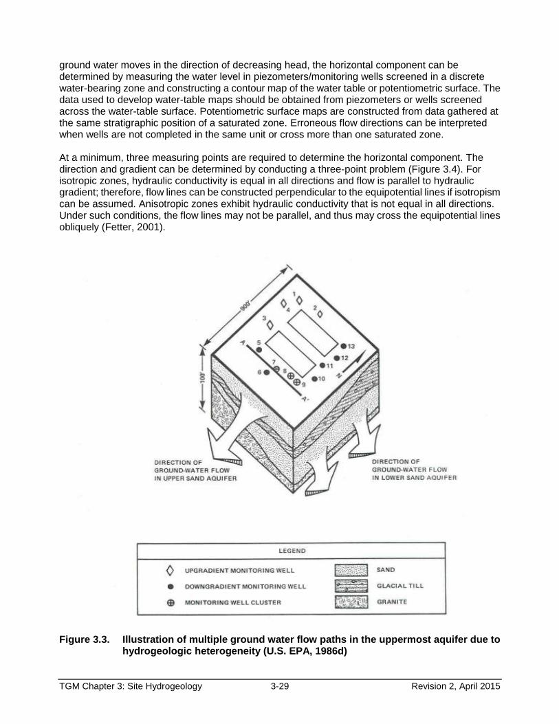
TGM Chapter 3: Site Hydrogeology 3-29 Revision 2, April 2015

ground water moves in the direction of decreasing head, the horizontal component can be determined by measuring the water level in piezometers/monitoring wells screened in a discrete water-bearing zone and constructing a contour map of the water table or potentiometric surface. The data used to develop water-table maps should be obtained from piezometers or wells screened across the water-table surface. Potentiometric surface maps are constructed from data gathered at the same stratigraphic position of a saturated zone. Erroneous flow directions can be interpreted when wells are not completed in the same unit or cross more than one saturated zone. At a minimum, three measuring points are required to determine the horizontal component. The direction and gradient can be determined by conducting a three-point problem (Figure 3.4). For isotropic zones, hydraulic conductivity is equal in all directions and flow is parallel to hydraulic gradient; therefore, flow lines can be constructed perpendicular to the equipotential lines if isotropism can be assumed. Anisotropic zones exhibit hydraulic conductivity that is not equal in all directions. Under such conditions, the flow lines may not be parallel, and thus may cross the equipotential lines obliquely (Fetter, 2001).

Figure 3.3. Illustration of multiple ground water flow paths in the uppermost aquifer due to

hydrogeologic heterogeneity (U.S. EPA, 1986d)

TGM Chapter 3: Site Hydrogeology 3-30 Revision 2, April 2015

(1) (2) Both the direction of ground-water movement and the hydraulic gradient can be determined if the following data are available for three wells located in any triangular arrangement such as that shown on sketch 1: 1. The relative geographic position of the wells. 2. The distance between wells. 3. The total head at each well. Steps in the solution are outlined below and illustrated in sketch (2): a. Identify the well that has the intermediate water

level (that is, neither the highest head nor the lowest head).

b. Calculate the position between the well having

the highest head and the well having the lowest head at which the head is the same as that in the intermediate well.

c. Draw a straight line between the intermediate well and the point identified in step b as being between the well having the highest head and that having the lowest head. The line represents a segment of the water level contour along which the total head is the same as that in the intermediate well.

d. Draw a line perpendicular to the water level

contour and through either the well with the highest head or the well with the lowest head. The line parallels the direction of ground water movement.

e. Divide the difference between the head of the

well and that of the contour by the distance between the well and the contour. The answer is the hydraulic gradient.

Figure 3.4. Estimation of flow direction and gradient by a 3-point problem (Heath, 1984)

TGM Chapter 3: Site Hydrogeology 3-31 Revision 2, April 2015

Use of three measuring points is appropriate only if a site is relatively small and the configuration of the water table or potentiometric surface is planar (Dalton et al., 2006). Lateral variations in hydraulic conductivity, localized recharge and drainage patterns, and other factors can cause the configuration to be non-planar. Also, a ground-water divide may be present that would not be detected with only a minimal number of measuring points. For large sites, it is recommended that at least 6 to 9 measuring points be utilized to provide a preliminary estimate of flow direction within a target area. After several sets of data are collected and analyzed, the need for additional wells/piezometers can be evaluated. 3.6.1.2 Vertical Component and Interconnectivity In addition to considering the horizontal component of flow, an investigation and/or monitoring program should directly assess the vertical component and the interconnection between saturated zones. Gradient and the relative direction of the vertical component are determined by comparing water level measurements in well/piezometer clusters. The presence of vertical gradients can be anticipated in recharge or discharge areas or in areas underlain by a layered geologic sequence (especially where deposits of lower hydraulic conductivity overlie deposits of substantially higher hydraulic conductivity). In general, interconnection can be determined by pumping a lower zone and monitoring changes in water levels measured in zones above the pumped zone. The number of wells, pumping rate, length of tests, and method of data evaluation is dependent on site conditions. The design of pumping tests is discussed in TGM Chapter 4. Another technique to help determine hydraulic connection between zones is to compare their water quality. As ground water flows, it assumes a diagnostic composition as a result of interaction with subsurface materials (Fetter, 2001). It is important to note that within each zone, natural changes in water quality also occur with increasing contact time. Interconnectivity may also be observed by correlation of water levels with recharge events and use of environmental tracers. 3.6.1.3 Seasonal and Temporal Effects Regulated entities should identify and assess factors that may result in short- or long-term variation in ground water levels and flow direction. There may be more than one mechanism operating simultaneously. Table 3.13 provides a summary of the factors, which are classified according to whether they are natural or anthropogenic; whether they produce fluctuations in confined or unconfined zones; and whether they are short-lived, diurnal, seasonal, or long-term. These phenomena have been discussed in detail by Freeze and Cherry (1979). Continued monitoring and evaluation of ground water levels are necessary to detect changes in the flow regime. At a minimum, quarterly measurements should be made to assess seasonal effects. More frequent determinations may be necessary to assess diurnal, short-lived, and anthropogenic effects. Multiple years of data collection may be necessary to evaluate seasonal effects.

TGM Chapter 3: Site Hydrogeology 3-32 Revision 2, April 2015

3.6.1.4 Anthropogenic Effects Ground water flow direction can be affected by anthropogenic influences such as pumping wells, leaking water lines, and buried pipelines. These influences need to be assessed to determine the movement of chemicals that have been released. Pumpage may be seasonal or dependent on water consumption patterns. For sites where variations in pumping rates occur in the vicinity, frequent measurements may be needed to detect changes in flow patterns. External loading in the form of passing trains and construction blasting may lead to measurable, but short-lived, oscillations in water level recorders in confined ground water zones. 3.6.1.5 Potentiometric Maps Potentiometric surface maps are typically constructed to show horizontal ground water flow directions. Water-level elevation is plotted on a base map and linear interpolation of the data points is made to construct lines (contours) of equal elevation (Figure 3.5). The data used should be from well intakes located in the same hydrostratigraphic zone and at the same elevation. The water-table is a particular potentiometric surface for an unconfined aquifer. Water table maps should be based on elevations from wells screened across the water table. The flow direction for each zone may be determined by drawing flow lines perpendicular to the contours. A reliable interpretation of ground water flow must consider geologic data such as valley walls and interaction with surface water, etc. The greatest amount of interpretation is at the periphery of the data set. The interpretation should also consider water-quality data. For example, if contamination is present in wells that are not downgradient of a contaminant source, then further assessment may be necessary to determine whether there is off-site contamination, whether the interpreted flow direction is correct, or whether flow is affected by seasonal or anthropogenic influences. Computer programs and statistical techniques (for example, kriging), have been developed to assess ground water flow conditions. The approach and assumptions that underlie these methods should be thoroughly understood and the output from the computer should be critically reviewed to ensure that a consistent interpretation is being made (Dalton, et al., 2006). Ground water elevations in a discrete zone should be measured at regular intervals and maps constructed. The interval between measurements should be sufficient to adequately address potential seasonal and anthropogenic influences.

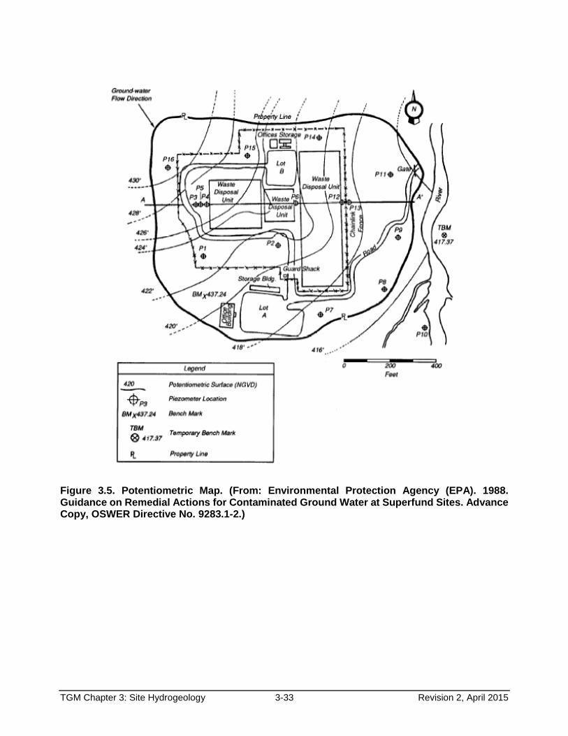
TGM Chapter 3: Site Hydrogeology 3-33 Revision 2, April 2015

Figure 3.5. Potentiometric Map. (From: Environmental Protection Agency (EPA). 1988. Guidance on Remedial Actions for Contaminated Ground Water at Superfund Sites. Advance Copy, OSWER Directive No. 9283.1-2.)

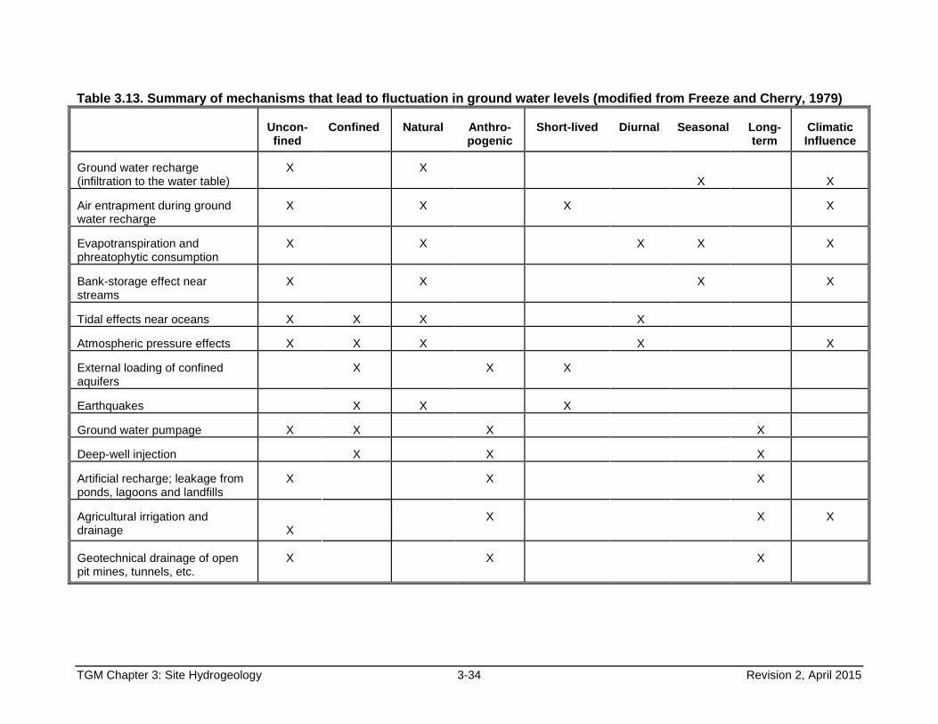
TGM Chapter 3: Site Hydrogeology 3-34 Revision 2, April 2015

Table 3.13. Summary of mechanisms that lead to fluctuation in ground water levels (modified from Freeze and Cherry, 1979)

Uncon-fined

Confined

Natural

Anthro- pogenic

Short-lived

Diurnal

Seasonal

Long- term

Climatic Influence

Ground water recharge (infiltration to the water table)

X

X

X

X Air entrapment during ground water recharge

X

X

X

X

Evapotranspiration and phreatophytic consumption

X

X

X

X

X

Bank-storage effect near streams

X

X

X

X

Tidal effects near oceans

X

X

X

X

Atmospheric pressure effects

X

X

X

X

X

External loading of confined aquifers

X

X

X

Earthquakes

X

X

X

Ground water pumpage

X

X

X

X

Deep-well injection

X

X

X

Artificial recharge; leakage from ponds, lagoons and landfills

X

X

X

Agricultural irrigation and drainage

X

X

X

X

Geotechnical drainage of open pit mines, tunnels, etc.

X

X

X

TGM Chapter 3: Site Hydrogeology 3-35 Revision 2, April 2015

3.6.2 Hydraulic Gradient Horizontal hydraulic gradient is the total change in head with change in distance in the direction of flow. The gradient generally is analogous to the slope of the potentiometric or water-table surface. Gradients can range from greater than 1 (near a point of discharge) to less than 0.0001, a value associated with extensive area of flat terrain and high hydraulic conductivity (Sara, 2003). The horizontal gradient can be determined by a 3-point problem as described in Figure 3.4 or by dividing the difference in head between two contour lines on a potentiometric map by the orthogonal distance between them. In addition to evaluating the horizontal component of hydraulic gradient, the vertical component should be investigated. The vertical component within a formation can be determined by comparing heads in well/piezometer clusters screened in that zone. Vertical gradients between zones can be determined if hydraulic connection exists. A site could exhibit different horizontal and/or vertical gradients depending on where measurements are taken. Gradients are influenced by the characteristics of the ground water zone (for example, hydraulic conductivity, thickness, etc.), boundary conditions (for example, rivers), precipitation, and anthropogenic influences (Sara, 2003). Hydraulic gradients should be provided as a range. 3.6.3 Porosity/Effective Porosity Porosity is the ratio of openings to the total volume of rock and soil. Since ground water moves and is stored within pores and fractures, porosity is important in describing flow and characterizing the quantity of contaminants that can be stored. Porosity (n) can be calculated by a variety of means. The most common is to calculate the percentage of total soil volume occupied by pores. This is done by calculating a soil’s bulk and particle density (Methods of Soil Analysis, 1986) and using:

Porosity (n) = [1 - (bulk density/particle density)] The bulk density is defined as the ratio of the mass of dry solids to the bulk volume of the soil and the particle density is the ratio of the solid particle mass to their total volume. Typical porosities are listed in Table 3.14. On average, particle densities of 2.65 g/cm3 are typical of sandy soils but decrease as the clay and organic matter content rise. Not all of the porosity is available for flow. Part will be occupied by static fluids being held to the soil/rock by surface tension or contained in dead end pore spaces. It is a function of the size of the molecules that are being transported to the relative size of the passageways that connect the pores. Effective porosity is difficult to measure and is typically selected by experience and intuition. Effective porosity is generally estimated based on the description and classification of subsurface materials and by total porosity, determined from lab tests or estimated from the literature. Tables 3.14 and 3.15 provide data that might be useful to this estimation. Peyton et al., (1986) found that even in lacustrine clay, water molecules could pass through all pore throats, so that effective porosity was essentially the same as porosity. This suggests that, for at least water, effective porosity may be considered equal to total porosity.

TGM Chapter 3: Site Hydrogeology 3-36 Revision 2, April 2015

For unfractured glacial till, it is recommended that 30 percent be used for ne in velocity calculations10. While a default value of one percent has been cited for clay (U.S. EPA, 1986c), this results in high rates that are intuitively incorrect. Primary flow through clay is known to be very low. The basis for one percent is specific yield determinations (Sara, 1994); however, laboratory column breakthrough tests done by Golder Associates (1990) indicated ne for till ranging from 0.26 to 0.35. This range compares favorably with the value for clays reported by Rawls et al. (1983) (Table 3.14). Ohio EPA’s experience is that use of 30 percent results in very conservative estimates of ground water movement through unfractured glacial till. 3.6.4 Hydraulic Conductivity Hydraulic conductivity11 (K) is a coefficient of proportionality describing the ease at which fluid can move through a permeable medium and is expressed in units of length per time. It is a function of properties of both the porous medium and the fluid. The K of geologic materials can vary from 1 to 1 x 10-13 m/s. Generally, finer-grained materials are characterized by lower values. Materials that contain a broad range of grain sizes (for example, glacial till) typically exhibit values lower than deposits with uniform grain size (for example, beach sands) (Sevee, 2006). The determination of K is also important not only as a parameter for determination of flow rate, but as a means for describing and comparing different units. A saturated zone may be described as either homogenous or heterogeneous and either isotropic or anisotropic according to the variability of K in space. A zone is homogeneous if K is independent of location, and is heterogeneous if it is dependent on location. If K is independent of the direction of measurement, the zone is isotropic. If it varies with direction, the zone is anisotropic. Anisotropy typically is the result of small-scale stratification such as bedding of sedimentary deposits and/or fractures. In bedded deposits, K is typically highest in the direction parallel to bedding and smallest perpendicular to bedding. In general, K can be several orders of magnitude higher horizontally than vertically. Horizontal and vertical K should be determined for each discrete zone. The variation of K as a function of vertical position within each formation should be identified because such variations can create irregularities in ground water flow paths and rates.

10

It should be noted that the applicability of Darcy’s law to calculating primary flow velocity in fine-grained material is questionable. However, this currently is one of the best available tools to assist professionals in evaluating whether a confining unit provides protection to the underlying ground water. To further demonstrate that ground water has not/will not be affected by a potential contaminant source, other methods such as tracers may be helpful. 11 In many engineering texts, hydraulic conductivity is also known as the coefficient of permeability; as a result, the two terms are used interchangeably in hydrogeologic applications (Sevee, 2006).

TGM Chapter 3: Site Hydrogeology 3-37 Revision 2, April 2015

Table 3.14. Porosity and Effective Porosity of Common Soils (Rawls et al., 1983)a

Texture Mean Total Porosity

Mean Effective Porosity

Sand

0.437

0.417

Loamy Sand

0.437

0.401

Sandy Loam

0.453

0.412

Loam

0.463

0.434

Silt Loam

0.501

0.486

Sandy Clay Loam

0.398

0.330

Clay Loam

0.464

0.309

Silty Clay Loam

0.471

0.432

Sandy Clay

0.430

0.321

Silty Clay

0.479

0.423

Clay

0.475

0.385

a Based on published data for approximately 1200 soils (5,000 horizons) from 34 states.

Table 3.15. Range of percentage of porosity for various geologic materials GEOLOGIC MATERIALS

BOUWER

(1978)

TODD (1980)

FETTER (2001)

FREEZE AND

CHERRY (1979)

SEVEE (2006)

gravel, mixed

20-30

25-40

25-40

gravel, coarse

28

gravel, medium

32

gravel, fine

34

sand, mixed

25-50

25-50

15-48

sand, coarse

25-35

39

sand, medium

35-40

39

sand, fine

40-50

42

sand & gravel

10-30

25-50

silt

50-60

46

35-50

35-50

35-50

clay

50-60

42

33-60

40-70

40-70

limestone

10-20

30

0-20

0-20

karst limestone

5-50

5-50

shale

6

0-10

0-10

sandstone

5-30

33-37

5-30

5-40

TGM Chapter 3: Site Hydrogeology 3-38 Revision 2, April 2015

Several techniques exist for determining the K of geologic material. These include initial estimation, laboratory determination, and field tests. In general, the field is favored over the laboratory because results represent in-situ conditions. However, laboratory analysis may be sufficient for ascertaining vertical K. The appropriate application for each technique is discussed below. 3.6.4.1 Estimation Several methods exist to estimate K from engineering and geologic descriptions and from correlations between these properties and several commonly measured soil parameters (Dawson and Istok, 1991; Batu, 1998). However, estimation should be used only initially to help determine the most appropriate field technique. Values can be estimated by comparison of material to similar materials for which a value has been established. Figure 3.6 shows typical ranges. It must be noted that estimates for a specific material can vary over several orders of magnitude (Dawson and Istok, 1991). Values for K can be inferred from the grain-size distribution of an unconsolidated material. Numerous investigators have developed empirical formulas to compare grain size to hydraulic conductivity. Hazen (1911) related effective particle size to K such that:

K = C(D10)2

where:

K = hydraulic conductivity in cm/sec. D10 = particle size (measured in mm) below which ten percent of the cumulative sample

has a smaller size. C = constant ranging from 1 to 1.2 depending on the gradation of the sand.

This formula was developed for estimating the K of sand filters; therefore, use generally is limited to uniformly-graded sands. Other methods, such as the one developed by Fair and Hatch (1933), employ the entire grain size distribution curve. Other equations can be found in Batu (1998). Techniques using soil index properties also have been developed (Dawson and Istok, 1991; Alyomini and Sen, 1993).

TGM Chapter 3: Site Hydrogeology 3-39 Revision 2, April 2015

Figure 3.6. Hydraulic conductivity of selected geologic materials (Heath, 1984)

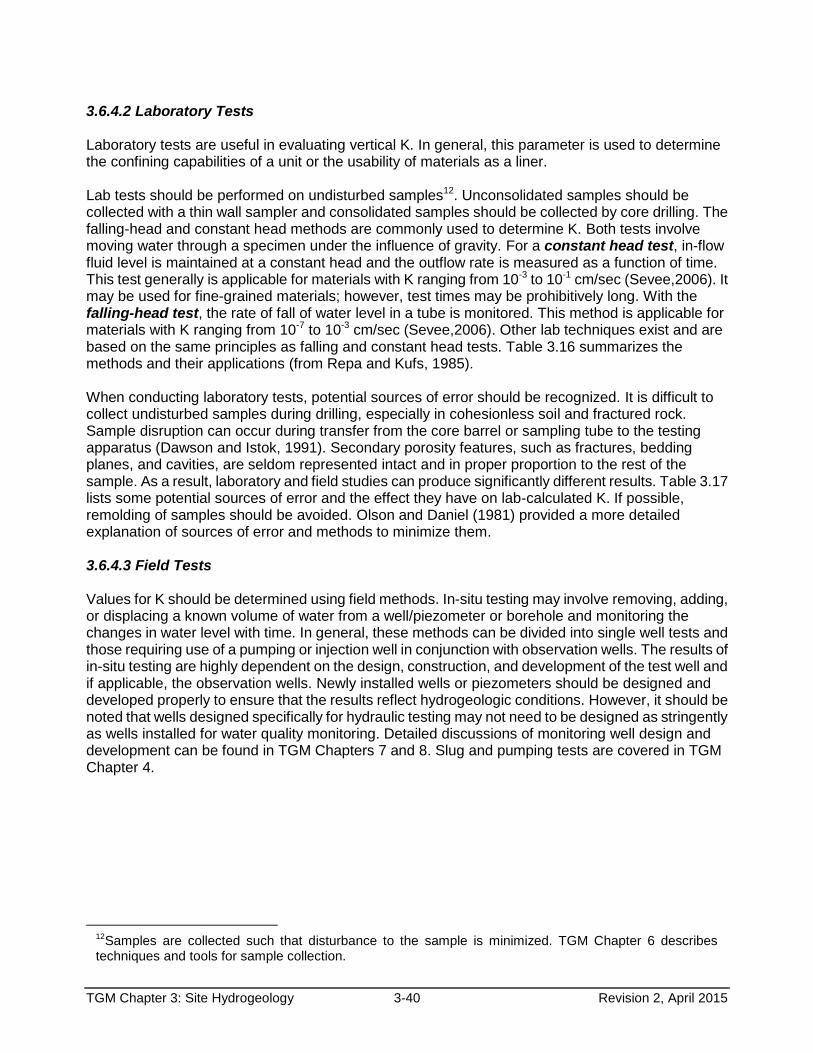
TGM Chapter 3: Site Hydrogeology 3-40 Revision 2, April 2015

3.6.4.2 Laboratory Tests Laboratory tests are useful in evaluating vertical K. In general, this parameter is used to determine the confining capabilities of a unit or the usability of materials as a liner. Lab tests should be performed on undisturbed samples12. Unconsolidated samples should be collected with a thin wall sampler and consolidated samples should be collected by core drilling. The falling-head and constant head methods are commonly used to determine K. Both tests involve moving water through a specimen under the influence of gravity. For a constant head test, in-flow fluid level is maintained at a constant head and the outflow rate is measured as a function of time. This test generally is applicable for materials with K ranging from 10-3 to 10-1 cm/sec (Sevee,2006). It may be used for fine-grained materials; however, test times may be prohibitively long. With the falling-head test, the rate of fall of water level in a tube is monitored. This method is applicable for materials with K ranging from 10-7 to 10-3 cm/sec (Sevee,2006). Other lab techniques exist and are based on the same principles as falling and constant head tests. Table 3.16 summarizes the methods and their applications (from Repa and Kufs, 1985). When conducting laboratory tests, potential sources of error should be recognized. It is difficult to collect undisturbed samples during drilling, especially in cohesionless soil and fractured rock. Sample disruption can occur during transfer from the core barrel or sampling tube to the testing apparatus (Dawson and Istok, 1991). Secondary porosity features, such as fractures, bedding planes, and cavities, are seldom represented intact and in proper proportion to the rest of the sample. As a result, laboratory and field studies can produce significantly different results. Table 3.17 lists some potential sources of error and the effect they have on lab-calculated K. If possible, remolding of samples should be avoided. Olson and Daniel (1981) provided a more detailed explanation of sources of error and methods to minimize them. 3.6.4.3 Field Tests Values for K should be determined using field methods. In-situ testing may involve removing, adding, or displacing a known volume of water from a well/piezometer or borehole and monitoring the changes in water level with time. In general, these methods can be divided into single well tests and those requiring use of a pumping or injection well in conjunction with observation wells. The results of in-situ testing are highly dependent on the design, construction, and development of the test well and if applicable, the observation wells. Newly installed wells or piezometers should be designed and developed properly to ensure that the results reflect hydrogeologic conditions. However, it should be noted that wells designed specifically for hydraulic testing may not need to be designed as stringently as wells installed for water quality monitoring. Detailed discussions of monitoring well design and development can be found in TGM Chapters 7 and 8. Slug and pumping tests are covered in TGM Chapter 4.

12Samples are collected such that disturbance to the sample is minimized. TGM Chapter 6 describes techniques and tools for sample collection.

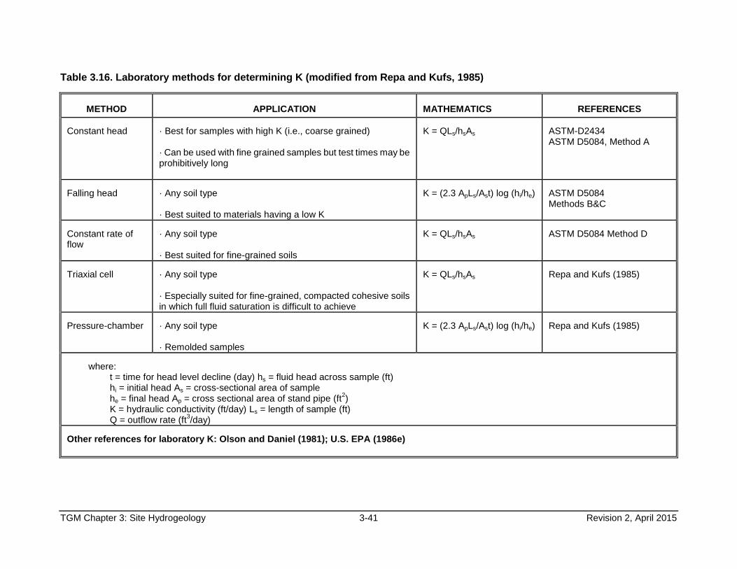
TGM Chapter 3: Site Hydrogeology 3-41 Revision 2, April 2015

Table 3.16. Laboratory methods for determining K (modified from Repa and Kufs, 1985)

METHOD APPLICATION

MATHEMATICS

REFERENCES

Constant head

· Best for samples with high K (i.e., coarse grained) · Can be used with fine grained samples but test times may be prohibitively long

K = QLs/hsAs

ASTM-D2434 ASTM D5084, Method A

Falling head

· Any soil type · Best suited to materials having a low K

K = (2.3 ApLs/Ast) log (hi/he)

ASTM D5084 Methods B&C

Constant rate of flow

· Any soil type · Best suited for fine-grained soils

K = QLs/hsAs

ASTM D5084 Method D

Triaxial cell

· Any soil type · Especially suited for fine-grained, compacted cohesive soils in which full fluid saturation is difficult to achieve

K = QLs/hsAs

Repa and Kufs (1985)

Pressure-chamber

· Any soil type · Remolded samples

K = (2.3 ApLs/Ast) log (hi/he)

Repa and Kufs (1985)

where:

t = time for head level decline (day) hs = fluid head across sample (ft) hi = initial head As = cross-sectional area of sample he = final head Ap = cross sectional area of stand pipe (ft

2)

K = hydraulic conductivity (ft/day) Ls = length of sample (ft) Q = outflow rate (ft

3/day)

Other references for laboratory K: Olson and Daniel (1981); U.S. EPA (1986e)

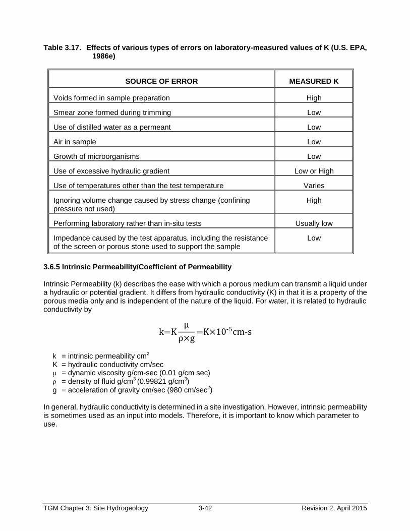
TGM Chapter 3: Site Hydrogeology 3-42 Revision 2, April 2015

Table 3.17. Effects of various types of errors on laboratory-measured values of K (U.S. EPA, 1986e)

SOURCE OF ERROR

MEASURED K

Voids formed in sample preparation

High

Smear zone formed during trimming

Low

Use of distilled water as a permeant

Low

Air in sample

Low

Growth of microorganisms

Low

Use of excessive hydraulic gradient

Low or High

Use of temperatures other than the test temperature

Varies

Ignoring volume change caused by stress change (confining pressure not used)

High

Performing laboratory rather than in-situ tests

Usually low

Impedance caused by the test apparatus, including the resistance of the screen or porous stone used to support the sample

Low

3.6.5 Intrinsic Permeability/Coefficient of Permeability

Intrinsic Permeability (k) describes the ease with which a porous medium can transmit a liquid under a hydraulic or potential gradient. It differs from hydraulic conductivity (K) in that it is a property of the porous media only and is independent of the nature of the liquid. For water, it is related to hydraulic conductivity by

k=Kμ

ρ×g=K×10-5cm-s

k = intrinsic permeability cm2 K = hydraulic conductivity cm/sec μ = dynamic viscosity g/cm-sec (0.01 g/cm sec) ρ = density of fluid g/cm3 (0.99821 g/cm3)

g = acceleration of gravity cm/sec (980 cm/sec2) In general, hydraulic conductivity is determined in a site investigation. However, intrinsic permeability is sometimes used as an input into models. Therefore, it is important to know which parameter to use.

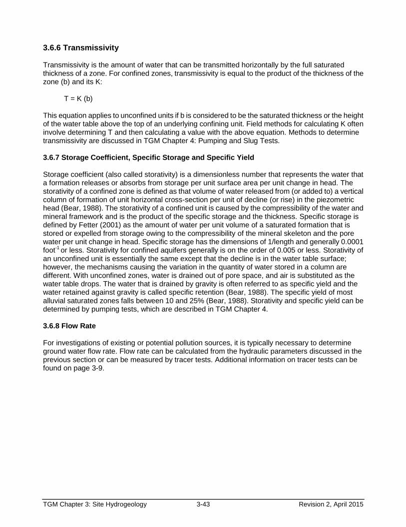
TGM Chapter 3: Site Hydrogeology 3-43 Revision 2, April 2015

3.6.6 Transmissivity

Transmissivity is the amount of water that can be transmitted horizontally by the full saturated thickness of a zone. For confined zones, transmissivity is equal to the product of the thickness of the zone (b) and its K:

T = K (b) This equation applies to unconfined units if b is considered to be the saturated thickness or the height of the water table above the top of an underlying confining unit. Field methods for calculating K often involve determining T and then calculating a value with the above equation. Methods to determine transmissivity are discussed in TGM Chapter 4: Pumping and Slug Tests. 3.6.7 Storage Coefficient, Specific Storage and Specific Yield Storage coefficient (also called storativity) is a dimensionless number that represents the water that a formation releases or absorbs from storage per unit surface area per unit change in head. The storativity of a confined zone is defined as that volume of water released from (or added to) a vertical column of formation of unit horizontal cross-section per unit of decline (or rise) in the piezometric head (Bear, 1988). The storativity of a confined unit is caused by the compressibility of the water and mineral framework and is the product of the specific storage and the thickness. Specific storage is defined by Fetter (2001) as the amount of water per unit volume of a saturated formation that is stored or expelled from storage owing to the compressibility of the mineral skeleton and the pore water per unit change in head. Specific storage has the dimensions of 1/length and generally 0.0001 foot-1 or less. Storativity for confined aquifers generally is on the order of 0.005 or less. Storativity of an unconfined unit is essentially the same except that the decline is in the water table surface; however, the mechanisms causing the variation in the quantity of water stored in a column are different. With unconfined zones, water is drained out of pore space, and air is substituted as the water table drops. The water that is drained by gravity is often referred to as specific yield and the water retained against gravity is called specific retention (Bear, 1988). The specific yield of most alluvial saturated zones falls between 10 and 25% (Bear, 1988). Storativity and specific yield can be determined by pumping tests, which are described in TGM Chapter 4. 3.6.8 Flow Rate For investigations of existing or potential pollution sources, it is typically necessary to determine ground water flow rate. Flow rate can be calculated from the hydraulic parameters discussed in the previous section or can be measured by tracer tests. Additional information on tracer tests can be found on page 3-9.

TGM Chapter 3: Site Hydrogeology 3-44 Revision 2, April 2015

3.6.8.1 Calculation from Hydraulic Parameters In general, ground water flow rate can be determined mathematically based on site-specific parameters. The following equation, derived from Darcy's law, generally is utilized:

V=Kdh

dlne

⁄

where:

V = mean ground water particle velocity (length/time) K = hydraulic conductivity (length/time) hd/dl = hydraulic gradient (length/length) ne = effective porosity (unitless)

As shown, velocity is proportional to hydraulic gradient and hydraulic conductivity and inversely proportional to effective porosity. Situations in which the derived equation may not apply include systems where: 1) ground water flows through materials with low hydraulic conductivity under an extremely low gradient; or 2) large amounts of water pass through conduits, thus possibly causing the flow to be turbulent (Freeze and Cherry, 1979). In fractured rock, interconnected discontinuities are considered to be the main passage for fluid flow. In general, two approaches might be followed when dealing with flow through fractured rocks: continuum or discontinuum. The continuum approach assumes that the fracture mass is hydraulically equivalent to a porous medium, thus Darcy’s Law as developed can be applied. If continuum conditions do not exist, the flow must be described in relation to individual fractures or fracture sets. The concept for flow in fractures is further developed in Freeze and Cherry (1979) and Domenico and Schwartz (1998). 3.6.8.2 Field Determination of Flow Rate Though tracer tests can be used to determine flow rates, they can be difficult to perform and are not often used. Borehole flow meters can measure incremental discharge along a screened or open-hole well during small scale pumping tests. Three types of flow meters include: impeller, heat-pulse, and electromagnetic. The heat and electromagnetic flow meters have no moving parts and are more sensitive. This sensitivity allows detection of vertical movement of water within the borehole under non-pumping conditions. Under pumping conditions, fracture zones contributing water to a borehole may be detected (U.S. EPA, 1991). 3.6.9 Saturated Zone Yield Saturated zone yield generally can be defined as the maximum sustained quantity of water supplied over a period of time to a properly constructed well. Determining yield often involves pumping wells at a specific rate to determine whether they can sustain that rate for a specified amount of time. Well construction, location of the well, and seasonal variations may affect the yield and may need to be considered. Also, the applicable program should be consulted to determine whether there are specific regulatory requirements or guidance on addressing yield. Yield may also be determined from single or multiple-well pumping tests. Pumping tests are

discussed in TGM Chapter 4.

TGM Chapter 3: Site Hydrogeology 3-45 Revision 2, April 2015

4.0 GROUND WATER USE DETERMINATION

It is often necessary to determine the ground water use in the vicinity of the area being investigated. 4.1 PUBLICLY AVAILABLE RECORDS An evaluation of records on file at Ohio EPA, ODNR, Department of Agriculture and the local Health Department can assist in determining past, current, or potential ground water use.

Ohio EPA, Division of Drinking and Ground Waters, (epa.ohio.gov/ddagw/), regulates public water systems. Information can be obtained from the Ohio EPA district offices (epa.ohio.gov/districts.aspx) on location and discharge rates of public water systems. In addition, information about drinking water source protection areas for a public water system using ground water can be obtained.

ODNR, Division of Soil and Water Resources, (soilandwater.ohiodnr.gov), is charged with collecting and maintaining well logs. The evaluation should include not only those logs for which the well locations have been mapped by ODNR on a USGS quadrangle, but also those well logs that are on file but have not been mapped by ODNR (herein referred to as unlocated logs). The physical location of the wells should be determined for the unlocated logs. The city and street address and/or driller’s location description can be used to help locate the well and determine if ground water has been used or potentially will be used in the vicinity of the area being investigated.

A review of county or other local health department records (www.odh.ohio.gov/~/media/ODH/ASSETS/Files/lhd/OHIO-LHDcontact.ashx) to determine whether well permits have been issued.

An inquiry of other local authorities with jurisdiction over installation of wells. Each quarry must file an annual water withdrawal report with the ODNR Division of Soil and

Water Resources, which can provide an estimate of ground water pumpage from the site.

4.2 SURVEYS Surveys for wells may also be useful in assessing ground water use. A survey may be as simple as a drive-by observation or as extensive as conducting a door-to-door or mail survey. Interviews or surveys of local drillers to determine whether they have installed wells and/or local water suppliers may help to determine the ground water use in the area. The “level of effort” needed for the survey is site-specific and dependent on the other documentation supporting the well location evaluation. 4.3 OTHER LINES OF EVIDENCE Other lines of evidence include:

An ordinance requiring residents/businesses to connect to the public drinking water system.

A ban on drilling water wells in the area.

A local requirement or ordinance requiring a permit for the installation of a water supply well. The weight of the above evidence is dependent on whether these can be, and have been effectively monitored and enforced by the local authority having the jurisdiction.

TGM Chapter 3: Site Hydrogeology 3-46 Revision 2, April 2015

5.0 ANALYSIS AND PRESENTATION OF HYDROGEOLOGIC INFORMATION

The data and information collected should be reviewed to determine whether the data quality objectives/requirements were met. This review should not only include data currently collected, but also include all field and laboratory data from previous investigations. Interpretation of field- and laboratory-measured environmental parameters should include a discussion of possible limitations of the method used. Basic assumptions for analytical techniques and methods should be evaluated to determine if site conditions meet assumptions. For example, the analysis of pumping test results should identify the approximate volume of the zone measured by the test and the underlying analytical or other equations used to compute aquifer parameters. If site conditions do not satisfy the assumptions, the effect on accuracy and interpretation of results should be stated. Ground water models to simulate flow and contaminant transport may be used to help define the site conditions. Ground water models represent or approximate a real system and are tools that help in the organization and understanding of hydrogeologic data or the prediction of future hydrogeologic events. Models are not a substitute for field investigations, but should be used as supplementary tools. Results are dependent on the quality and quantity of the field data available to define input parameters and boundary conditions (Wang and Anderson, 1982). Results should always be evaluated in context with the fundamental assumptions of the model and the adequacy of the input data. Additional information on the use of models can be found in TGM Chapter 14. To demonstrate that a site has been adequately characterized and proper procedures have been utilized, the data, methodologies and interpretations should be presented in a report. Components of the report should include, but should not be limited to, a written description, raw data, maps, cross sections and methodology. Any applicable regulations/rules should be consulted to determine if specific content and format are required. 5.1 WRITTEN DESCRIPTION A narrative description of the geology and nature and occurrence of ground water should include, at a minimum:

An evaluation of regional hydrogeology that includes depth to bedrock, characteristics of the major stratigraphic units, average yield of water wells within a one mile radius (logs for wells within one mile also should be submitted13), specific capacity, approximate direction of ground water flow, identification and estimation of the amount of recharge and discharge, geomorphology, and structural geology.

An accurate classification and description of the consolidated and unconsolidated materials at the site from the ground surface down to the base of the lowest saturated zone of concern. This may include:

o Hydraulic conductivity (vertical and horizontal). o Rock and soil types. o Thickness and lateral extent of units. o Porosity/effective porosity and bulk density. o Moisture content.

13

The radial distance may be specified by program requirements. For example, some CERCLA projects may need a 4 mile radius.

TGM Chapter 3: Site Hydrogeology 3-47 Revision 2, April 2015

o The attenuation capacity and mechanism of natural earth materials (such as ion exchange capacity, organic carbon content, mineral content, soil sorptive capacity, storage capacity, and/or pH).

A site-specific description of structural geology and geomorphology.

A site-specific description of the occurrence of ground water at the site, including:

o Identification of saturated zones, including depth and lateral and vertical extent. o Identification of zones of high K that may act as preferential pathways. o Identification of zones of low K that may act as barriers to contaminants. o Ground water flow direction and rates (including sample calculations). o Effects of stratification on saturated and unsaturated flow. o Description of the interconnection between saturated zones and surface water. o Description of recharge and discharge areas.

Fluctuations in ground water levels and their effects on flow direction.

Description of the relationship of the proposed/existing waste management unit to ground water occurrence and site geology.

5.2 RAW DATA All raw data collected during the hydrogeologic investigation should be included in the report. This should include, but not be limited to:

Boring/Geologic Logs: Logs should be provided for all borings. They should be complete technical records of conditions encountered and should include results of laboratory analyses, field identifications, descriptive text, and graphics. Depths/heights should be recorded in fractions (tenths). Logs should be uniform and legible for potential reproduction and submission and should contain, at a minimum, the following information:

o Site name and site-specific coordinates.

o The name of the responsible party, the driller, and the on-site geologist.

o Method of drilling.

o Boring identification number and coordinates.

o Date started, date completed, and date abandoned or converted into a well.

o Depth of boring.

o Surface elevation based on Mean Sea Level (MSL) or fixed referenced.

o Method and location of all in-situ sampling.

o Condition of samples, percent recovery, blow counts, moisture content, etc.

o Materials classification, both field and laboratory.

o Depth to water, water-bearing zones and laboratory permeability results.

o Color and/or stains.

o Presence of structural features, such as fractures, solution cavities, or bedding.

o Drilling observations, such as loss of circulation, rig chatter, and heaving sands o General (weather, field monitoring equipment, etc.).

Well Construction Logs: Construction logs should be provided for all wells and piezometers used to obtain water level measurements and ground water samples. Information that should be included is listed in TGM Chapter 7. Logs for all wells installed must be submitted to the

TGM Chapter 3: Site Hydrogeology 3-48 Revision 2, April 2015

ODNR, Division of Soil and Water Resources (Ohio Revised Code (ORC) 1521.05). Driller contractors may register with ODNR to file water well and drilling reports online (www.dnr.state.oh.us/tabid/3252/Default.aspx).

Ground Water Elevation Measurements: All ground water elevations should be submitted in tabulated form. ASTM D6000 describes basic tabular and graphic methods of presenting data.

Field Test Data: Raw data from in-situ hydraulic tests should be submitted with a report. General information that should be submitted is provided in TGM Chapter 4.

5.3 CROSS SECTIONS An adequate number of cross-sections should be provided. Various orientations (for example, in direction of ground water flow and orthogonal to ground water flow) should be used. Each cross-section should depict, at a minimum:

Depth, thickness, classification, and hydraulic characteristics of each unit.

Fill boundaries and thickness.

Water table and/or potentiometric surface.

Structures such as zones of fracturing that influence water movement.

Zones of higher K that may influence ground water flow.

Zones of lower K that may restrict and/or attenuate ground water flow.

Location and depth of each boring and/or monitoring well screen.

Orientation of cross-section. o Horizontal and vertical scales. o Location of proposed or existing waste management areas. o Legend.

5.4 MAPS All maps should be legible, have an accurate scale, north arrow and a legend that contains symbols used on the map. All appropriate locations mentioned in the text should be clearly labeled. Information on the map should be in agreement with data discussed in the text, tables, or in other illustrations. The following maps may assist in demonstrating site hydrogeology:

A surface topography map depicting (at a minimum) streams, wetlands, depressions and springs. The map should be constructed by a qualified professional and should provide contour intervals at a level of detail appropriate for the investigation (for example, two-foot intervals). The map should depict the location of all borings, monitoring wells and cross-sections. Employment of a conventional or photogrammetric survey company that develops topographic maps by obtaining aerial data often is necessary. Aerial data can be supplemented by data obtained from stereoscopic maps, wetland inventory maps, USGS topographic maps, etc.

A detailed facility map depicting anthropogenic features, including property lines (with owners of adjacent properties clearly marked), location of all potential contaminant disposal areas, buildings, and utility lines.

TGM Chapter 3: Site Hydrogeology 3-49 Revision 2, April 2015

Ground water elevation contour maps for each zone of concern, with actual measurements at each well/piezometer. Contour lines within the area represented by the data should be represented with a solid line. Any interpretation outside the area should be represented with a dotted or dashed line. An explanation of flow direction and a justification of the extrapolation of flow outside the area defined by the data points should be included in the narrative portion of the report. Flow direction and date water-level measurements obtained also should be depicted.

5.5 METHODOLOGY The methodology used to evaluate site hydrogeology should be described. This includes, but may not be limited to:

Number, location, and depth of borings and monitoring wells or piezometers.

Well and piezometer construction and development.

Characterization of soil and rock samples.

Definition of saturated zones and potential confining units.

Rationale for use of indirect methods such as geophysics.

TGM Chapter 3: Site Hydrogeology 3-50 Revision 2, April 2015

6.0 REFERENCES Aley, T. 2002. Groundwater Tracing Handbook. Ozark Underground Laboratory. Protem, MO. Alley, W.M. (editor). 1993. Regional Ground-Water Quality, Van Nostrand Reinhold, New York, New

York. Alyamani, M.S., and Sen Z. 1993. Determination of Hydraulic Conductivity From Complete Rain-Size

Distribution Curves. Ground Water. V31(4). p551-555. ASTM Standard D422-63 (2002) Standard Methods for Particle-Size Analysis of Soils. ASTM

International, West Conshohocken, Pennsylvania. ASTM Standard D854-10. Standard Methods For Specific Gravity of Soils. ASTM International, West

Conshohocken, Pennsylvania. ASTM, Standard 1556-07. Standard Method for Density of Soils in Place by Sand Cone Method.

ASTM International, West Conshohocken, Pennsylvania. ASTM, Standard 1557-09. Standard Methods for Laboratory Compaction Characteristics Using

Modified Effort (56,000 ft-lb/ft3 (2,700 KN/m/m3) ASTM International, West Conshohocken, Pennsylvania.

ASTM Standard D2167-08. Standard Method for Density and Unit Weight of Soil in Place by Rubber

Balloon Method. ASTM International, West Conshohocken, Pennsylvania. ASTM, Standard D2216-10. Standard Method For Laboratory Determination of Water (Moisture)

Content of Soils, Rock, by Mass. ASTM International, West Conshohocken, Pennsylvania. ASTM, Standard D2434.68(2006) Standard Method for Permeability of Granular Soils (Constant

Head). ASTM International, West Conshohocken, Pennsylvania. ASTM Standard D2487-11. Standard Method For Classification of Soils for Engineering Purposes

(Unified Soil Classification System). ASTM International, West Conshohocken, Pennsylvania. ASTM, Standard D2488-09a. Standard Method For Description and Identification of Soils (Visual

Manual Procedure). ASTM International, West Conshohocken, Pennsylvania. ASTM, Standard D2937-10. Standard Method For Density of Soil in Place by Drive Cylinder Method.

ASTM International, West Conshohocken, Pennsylvania. ASTM, Standard D3385-09. Standard Method For Infiltration Rate of Soils in Field Using

Double-Ring Infiltrometers ASTM International, West Conshohocken, Pennsylvania. ASTM, Standard D3441-05 Standard Method For, Cone Penetration Tests of Soils. ASTM

International, West Conshohocken, Pennsylvania. ASTM, Standard D4318-10. Standard Test Method for Liquid Limit, Plastic Limit, and Plasticity Index

for Soils. ASTM International, West Conshohocken, Pennsylvania. ASTM Standard D4643-08 Standard Test Method for Determination of Water (Moisture) Content of

Soil by Microwave Oven Heating. ASTM International, West Conshohocken, Pennsylvania.

TGM Chapter 3: Site Hydrogeology 3-51 Revision 2, April 2015

ASTM, Standard 4943-08. Standard Method for Shrinking Factors of Soils by Wax Method. ASTM

International, West Conshohocken, Pennsylvania. ASTM, Standard D4959-07 Standard Method for Determination of Water (Moisture) Content of Soils

by Direct Heating Methods. ASTM International, West Conshohocken, Pennsylvania. ASTM Standard D4972-01(2007) Standard Tests Method for pH in Soils. ASTM International, West

Conshohocken, Pennsylvania. ASTM, Standard D5084-10 Standard Method For Measurement of Hydraulic Conductivity of

Saturated Porous Materials Using a Flexible Wall Permeameter. ASTM International, West Conshohocken, Pennsylvania.

ASTM Standard D5093-02(2008) Standard Method For Field Measurement of Infiltration Using a

Double Ring Infiltrometer With a Sealed Inner Ring. ASTM International, West Conshohocken, Pennsylvania.

ASTM Standard D5778-07. Standard Test Method for Performing Electronic Friction Cone and

Piezocone Penetration Testing of Soils. ASTM International, West Conshohocken, Pennsylvania.

ASTM Standard D6000-96 (2008). Standard Method for Presentation of Water-Level Information

From Ground-Water Sites ASTM International, West Conshohocken, Pennsylvania. ASTM Standard D6031 / D6031M - 96(2010)e1 Standard Test Method for Logging In Situ Moisture

Content and Density of Soil and Rock by the Nuclear Method in Horizontal, Slanted, and Vertical Access Tubes. ASTM International, West Conshohocken.

ASTM Standard D6565-00(2005) Standard Test Method for Determination of Water (Moisture)

Content of Soil by the Time Domain Reflectometry (TDR) Method ASTM International, West Conshohocken, Pennsylvania.

ASTM Standard D6780-05. Standard Test Method for Water Content and Density of Soils in Place by

Time Domain Reflectometry (TDR). ASTM International, West Conshohocken, Pennsylvania. ASTM Standard D6938-10. Standard Test Method for In-Place Density and Water Content of Soil

and Soil Aggregate by Nuclear Methods (Shallow Depth). ASTM International, West Conshohocken, Pennsylvania.

ASTM Standard D7503-10. Standard Test Method for Measuring the Exchange Complex and Cation

Exchange of Inorganic Fine Grained Soils. ASTM International, West Conshohocken, Pennsylvania.

Baehr, T. R., and W. L. Turley, 2000, Seasonal and Temporal Water Level Trends in Glacial Till

Deposits (Abstract): in A Conference on Fractured Glacial Tills, R. J. Haefner, Ed., Water Management Association of Ohio Spring Conference, May 9-10, 2000, Columbus, Ohio, p. 22.

Barari, A., and L. S. Hedges, 1985, Movement of Water in Glacial Till: in Proceedings of the 17th

International Congress, International Association of Hydrogeologists, Hydrogeology of Rocks of Low Permeability, International Association of Hydrogeologists, pp. 129-136.

TGM Chapter 3: Site Hydrogeology 3-52 Revision 2, April 2015

Batu, V., 1998, Aquifer Hydraulics: A Comprehensive Guide to Hydrogeologic Data Analysis, John Wiley, New York.

Bear, J. 1988. Dynamics of Fluids in Porous Media.,Dover Publications. New York. Benson, R. C.2006. Second Edition. Remote Sensing and Geophysical Methods for Evaluation of

Subsurface Conditions. In: D. M. Nielsen (editor), Practical Handbook of Environmental Site Characterization Ground-Water Monitoring.Taylor & Francis. Boca Raton, Florida. pp. 249-295.

Black, C. A. (editor). 1965a. Methods of Soil Analysis. Part 1. Physical and Mineralogical Properties,

Including Statistics of Measuring Samples. Society of Agronomy Inc. Madison, Wisconsin. Black, C. A. (editor). 1965b. Methods of Soil Analysis. Part 2. Chemical and Microbiological

Properties. American Society of Agronomy. Madison, Wisconsin. Boulding, J.R. 1995. Soil, Vadose Zone, and Ground-Water Contamination-Assessment,

Prevention, and Remediation. Lewis Publishers. Bouwer, H. 1978. Groundwater Hydrology. McGraw-Hill Book Company. New York. Bradbury, K. R., Desaulniers, D. S., Connell, D. E., and R. G. Hennings, 1985, Groundwater

Movement Through Clayey Till, Northern Wisconsin, USA: in Proceedings of the 17th International Congress, International Association of Hydrogeologists, Hydrogeology of Rocks of Low Permeability, International Association of Hydrogeologists, pp. 405-416.

Bradbury, K.R., and M.A. Muldoon, 1990, Hydraulic Conductivity Determinations in Unlithified

Glacial and Fluvial Materials: in Ground Water and Vadous Zone Monitoring, ASTM Special Technical Publication 1053. D.M. Nelson and A.I. Johnson, Eds., p138-151.

Bruner, D. R., and A. J. Lutenegger, 1993, Measurement of Saturated Hydraulic Conductivity in

Fine-Grained Glacial Tills in Iowa: Comparison of In Situ and Laboratory Methods: in Hydraulic Conductivity and Waste Contaminant Transport in Soils, ASTM STP 1142, D. E. Daniel and S. J. Trautwein, Eds., American Society for Testing and Materials, Philadelphia.

Cravens, S. J., and L. C. Ruedisili. 1987. Water Movement in Till of East-Central South Dakota:

Ground Water, Vol. 25, No. 5 pp. 555-561. Cook, P. and A.L. Herzeg (editors). 2000. Environmental Tracers in Subsurface Hydrogeology.

Kluwer Academic Publishers. Boston, Massachusetts. Compton, R.R. 1985. Geology in the Field. John Wiley and Son. New York.

Dalton, M. G., B. E. Huntsman, and K. Bradbury. 2006. Acquisition and Interpretation of Water-Level Data. In: D. M. Nielsen (editor), Practical Handbook of Environmental Site Characterization and Ground-Water Monitoring. Taylor & Francis. Boca Raton, Fl. pp. 883-911.

Davis, S. N., D. J. Campbell, H. W. Bently, and T. J. Flynn. 1985. Ground Water Tracers.

Cooperative Agreement CR-80036, U.S. Environmental Protection Agency. National Ground Water Association, Dublin, OH.

TGM Chapter 3: Site Hydrogeology 3-53 Revision 2, April 2015

D’Astous, A. Y., Ruland, W. W., Bruce, J. R. G., Cherry, J. A., and R. W. Gillham, 1989, Fracture Effects in the Shallow Groundwater Zone in Weathered Sarnia-Area Clay: Can. Geotech. J., Vol 26., pp. 43-56.

Dawson, K. and J. D. Istok. 1991. Aquifer Testing, Design and Analysis of Pumping and Slug Tests.

Lewis Publishers, Inc. Chelsea, Michigan. Döll, P., and W. Schneider, 1995, Lab and Field Measurements of the Hydraulic Conductivity of

Clayey Silts: Ground Water, Vol. 33, No. 6, pp. 884-891. Domenico, P.A. and F.W. Schwartz. 1997. Second Edition. Physical and Chemical Hydrogeology.

John Wiley and Sons. New York. Fair, G. M., and L. P. Hatch. 1933. Fundamental Factors Governing the Streamline Flow of Water

Through Sand. Journal of American Water Works Association. Vol. 25, No. 11, pp. 1551-1561. Fetter, C. W. 2001. Applied Hydrogeology. Fourth Edition. Prentice Hall. Uper Saddle River, New

Jersey. Field, M.S., R.G. Wilhelm, J.F. Quinlan, and T.J Aley. 1995. An Assessment of the Potential Adverse

Properties of Fluorescent Tracer Dyes Used for Groundwater Tracing. U.S. Environmental Protection Agency, National Center and the office of Radiation and Indoor Air. Washington D.C. Quinlan and Associates Inc, Nashville, TN. Ozark Underground Laboratory, Protem, MO.

Freeze, R. A. and J. A. Cherry. 1979. Groundwater. Prentice-Hall Inc. Englewood Cliffs, New Jersey. Gerber, R. E., and K. Howard, 2000, Recharge Through a Regional Till Aquitard: Three-Dimensional

Flow Model Water Balance Approach: Ground Water, Vol. 38, No. 3, pp. 410-422. Golder Associates, Inc. 1990. Final Report on Breakthrough and Leachate Compatibility Testing of

Typical Clay Liner Materials, Adams Center Facility, Fort Wayne, Indiana. Prepared for Chemical Waste Management of Indiana, Inc.

Hazen, A. 1911. Discussion of "Dams on Sand Foundation" by A. C. Koenig. Transactions American

Society of Civil Engineers. Vol. 73, pp. 199-203. Heath, R. C. 1984. Basic Ground-Water Hydrology. U.S. Geological Survey Water-Supply Paper

2200. United States Government Printing Office. Alexandria, Virginia. Hendry, M. J., 1988, Hydraulic Conductivity of a Clay Till in a Prairie Region of Canada: Ground

Water, Vol. 26, No. 5, pp. 607-614 Hendry, M. J., 1982, Hydraulic Conductivity of a Glacial Till in Alberta: Ground Water, Vol. 20, No. 2,

pp. 162-169. Hendry, M. J., Cherry, J. A., and E. I. Wallick, 1986, Origin and Distribution of Sulfate in a Fractured

Till in Southern Alberta, Canada: Water Resources Research, Vol. 22, No. 1, pp. 45-61 Holtz, R. D. and W. D. Kovacs, 1981. An Introduction to Geotechnical Engineering. Prentice-Hall.

Englewood Cliffs, New Jersey.

TGM Chapter 3: Site Hydrogeology 3-54 Revision 2, April 2015

Jackson, J.A., 1997, Glossary of Geology (4th Edition): American Geological Institute, Alexandria, Virginia).

Javandel, I. 1984. Methods of Evaluating Vertical Ground Water Movement. Earth Science Division.

Lawrence Berkeley Laboratory. University of California, Berkeley, California. Jones, L., 1993, A Comparison of Pumping and Slug Tests for Estimating the Hydraulic Conductivity

of Unweathered Wisconsian Age Till in Iowa: Ground Water, Vol. 31, No. 6, pp. 896-904. Jury, W. A. 1986. Adsorption of Organic Chemicals Onto the Soil. In: S. C. Hern and S. M. Melancon

(editors), Vadose Zone Modeling of Organic Pollutants. Lewis Publishers Inc. Chelsea, Michigan. pp. 177-190.

Kazemi, Gholam A. J.H. Lehr, And Pierre Perrochet. 2006. Ground Water Age. John Wiley and

Sons. Hobken, New Jersy. Keller, C. K., van der Kamp, G., Cherry, J. A., 1991, Hydrogeochemistry of a Clayey Till - 1. Spatial

Variability: Water Resources Research, Vol. 27, No. 10, pp. 2543-2554. Keller, C. K., van der Kamp, G., Cherry, J. A., 1989, A Multiscale Study of the Permeability of a Thick

Clayey Till: Water Resources Research, Vol. 25, No. 11, pp. 2299-2317. Keller, C. K., van der Kamp, G., Cherry, J. A., 1988, Hydrogeology of Two Saskatchewan Tills, I.

Fractures, Bulk Permeability, and Spatial Variability of Downward Flow: Journal of Hydrology, Vol. 101, pp. 97-121.

Keller, C. K., van der Kamp, G., Cherry, J. A., 1986, Fracture Permeability and Groundwater Flow in

Clayey Till near Saskatoon, Saskatchewan: Can. Geotech J., Vol. 23, pp. 229-240. Kerfoot, W. B. 1988. Monitoring Well Construction and Recommended Procedures for Direct

Ground-Water Flow Measurements Using a Heat-Pulsing Flowmeter. In: A. G. Collins and A. I. Johnson (editors), Ground-water Contamination: Field Methods. ASTM Special Technical Publication 963. Philadelphia, Pennsylvania. pp. 146-161.

Keys, W.S. and L.M. MacCary. 1971. Techniques of Water Resource Investigation of the Unites States Geological Survey, Chapter E1: Application of Borehole Geophysics to Ground Water Investigations. U.S. Geological Survey. Book 2: Collection of Environmental Data. U.S. Government Printing Office. Washington D.C.

Kinner, N.E., R.W. Masters, and L.B. Fournier. 2005. Fractured Rock: State of the Science and

Measuring Success in Remediation. National Ground Water Association. Source: http://clu-in.org/fracrock.

Kulander, B.R., C.C. Barton, and S.L. Dean. 1990. Fracture Core Analysis: Interpretation, Logging,

and Natural and Induced Fractures in Core. American Association of Petroleum Geologists. Methods in Exploration Series, No. 8. Tulsa, Oklahoma.

McKay, L.D.; D.J. Balfour, J.A. Cherry. 1998. Lateral Chloride Migration from a Landfill in Fracture

Clay Rich Glacial Deposit. Ground Water. Volume 36, No. 6, pp. 988-999.

TGM Chapter 3: Site Hydrogeology 3-55 Revision 2, April 2015

Nielsen, D., G.L. Nielsen, and L.M. Preslo. 2006 (Second Edition). Environmental Site Characterization. In: D. M. Nielsen (editor), Practical Handbook of Environmental Site Characterization Ground-Water Monitoring.Taylor & Francis. Boca Raton, Florida. pp. 35-2005.

Olson, R. E. and D. F. Daniel. 1981. Measurement of Hydraulic Conductivity of Fine-Grained Soils.

In: T.F. Zimmie and C. O. Riggs (editors), Permeability and Groundwater Contaminant Transport. ASTM Special Publication 746. Philadelphia, Pennsylvania. pp. 18-64.

Payton, G.R., J.P. Gibb, M.H. LeFaivre, J.D. Ritchey, S.L. Burch, M.J. Barcelona. 1986. Effective

Porocity of Geologic Materials. Proceedings of the Twelfth Annual Research Symposium. U.S. EPA. EPA/600-9-86:21-8.

Plummer, L.N. and E. Busenberg. 2000. Chapter 15: Chlorofluorocarbons. In P. Cook and A.L.

Herczeg (editors): Environmental Tracers in Subsurface Hydrology. Kluwer Academic Publishers. Boston, Massachusetts.

Presley, D. and Thien, S. 2008. Estimating Soil Texture by Feel: Kansas State University

Department of Agronomy, MF-2852. Prudic, D. E., Hydraulic Conductivity of a Fine-Grained Till, Cattaraugus County, New York, 1982:

Ground Water, Vol. 20, No. 2, pp. 194-204. Rawls, W. J., D. L. Brakensiek, and N. Miller. 1983. Green-Ampt Infiltration Parameters from Soils

Data. ASCE Journal of Hydraulic Engineering. Vol. 9, No. 102. Repa, E. and C. Kufs. 1985. Leachate Plume Management. Hazardous Waste Engineering

Research Laboratory. Office of Solid Waste and Emergency Response. U.S. Environmental Protection Agency. EPA/540/2-85/004.

Robertson, P. K. and R. G. Campanella. 1986. Guidelines For Use and Interpretation of Electric

Cone Penetration Tests. Third Edition. Hogentogler and Company. Gaithersburg, Maryland. Ruda, T. and J. Farrar. 2006. Environmental Drilling for Soil Sampling, Rock Coring, Monitoring Well

Drilling, Borehole Logging and Monitoring Well Installation. In: D. M. Nielsen (editor), Practical Handbook of Environmental Site Characterization Ground-Water Monitoring. Taylor & Francis Group, LLC. Boca Raton, Florida. pp. 297-344.

Rudolph, D. L., Cherry, J. A., and R. N. Farvolden, 1991, Groundwater Flow and Solute Transport in

Fractured Lacustrine Clay Near Mexico City: Water Resources Research, Vol. 27, No. 9, pp. 2187-2201.

Ruland, W. W., Cherry, J. A., and S. Feenstra, 1991, The Depth of Fractures and Active

Ground-Water Flow in a Clayey Till Plain in Southwestern Ontario: Ground Water, Vol. 29, No. 3, pp. 405-417

Sara, M.C. 2003. Site Assessment and Remediation Handbook. Second Edition. CRC Press, Lewis

Publications. pp. Sevee, J. 2006. Second Edition. Methods and Procedures for Defining Aquifer Parameters. In: D. M.

Nielsen (editor), Practical Handbook of Environmental Site Characterization Ground-Water Monitoring. Taylor & Francis Group, LLC. Boca Raton, Florida. pp. 913-958.

TGM Chapter 3: Site Hydrogeology 3-56 Revision 2, April 2015

Simpkins, W. W., and K. R. Bradbury, 1992: Journal of Hydrology, Vol. 132, pp. 283-319. Smolley, M. and J. C. Kappmeyer. 1991. Cone Penetrometer Tests and Hydropunch Sampling: A

Screening Technique for Plume Definition. Ground Water Monitoring Review. Vol. 11, No. 2, pp. 101-106.

Solomon, D.K. and P.G. Cook. 2000. 3H and 3He. In P. Cook and A.L. Herczeg (editors):

Environmental Tracers in Subsurface Hydrology. Kluwer Academic Publishers. Boston, Massachusetts.

Strobel, M. L., 1993, Hydraulic Properties of Three Types of Glacial Deposits In Ohio: U.S.

Geological Survey Water-Resources Investigations Report 92-4135. Todd, D. K. and L.W. Mays. 2004. Ground Water. Third Edition. John Wiley and Sons. New York. U.S. EPA. 2003. Tracer-Test Planning Using the Efficient Hydrologic Tracer-Test Design (EHTD)

Program EPA/600/R-03/034 National Center for Environmental Assessment–Washington Office of Research and Development U.S. Environmental Protection Agency. Washington, DC 20460

U.S. EPA. 1998a. Estimation of Infiltration Rate in the Vadose Zone: Compilation of Simple

Mathematical Models. Volume 1. United States Environmental Program, National Risk Management Research Laboratory. EPA/600/R-97/128a. Ada, Ok.

U.S. EPA. 1998b. Estimation of Infiltration Rate in the Vadose Zone: Compilation of Simple

Mathematical Models. Volume 11. United States Environmental Program, National Risk Management Research Laboratory. EPA/600/R-97/128b. Ada, Ok.

U.S. EPA. 1997. Expedited Site Assessment Tools for Underground Storage Tanks Sites. A Guide

for Regulators. U.S. Environmental Protection Agency, Solid and Emergency Response. EPA 510-B-97-001.

U.S. EPA 1996. Guidelines for Wellhead and Springhead Protection Area Delineation in Carbonate

Rocks. United States Environmental Protection Agency. Region 4, Atlanta, Georgia. U.S. EPA. 1992. RCRA Ground-Water Monitoring Draft Technical Guidance. Office of Solid Waste.

U.S. Environmental Protection Agency. Washington, D.C. U.S. EPA.1991. Site Characterization for Subsurface Remediation. Office of Research and

Development. EPA/625/4-91/026. U.S. EPA. 1987. A Compendium of Superfund Field Operations Methods. Vol. 1 and 2. EPA/540/P-

87/001a and 001b. Office of Emergency and Remedial Response. Washington, D.C. U.S. EPA. 1986a. Cation-Exchange Capacity of Soils (Ammonium Acetate). In: Test Methods For

Evaluating Solid Waste. SW846, Method 9080. Office of Solid Waste and Emergency Response. Washington, D.C.

U.S. EPA. 1986b. Cation-Exchange Capacity of Soils (Sodium Acetate). In: Test Methods for

Evaluating Solid Waste. SW846, Method 9081. Office of Solid Waste and Emergency Response. Washington, D.C.

TGM Chapter 3: Site Hydrogeology 3-57 Revision 2, April 2015

U.S. EPA 1986c. Criteria for Identifying Areas of Vulnerable Hydrogeology Under the Resource Conservation and Recovery Act. [Statutory Interpretive Guidance. Guidance Manual for Hazardous Waste Land Treatment, Storage and Disposal Facilities.] Interim Final. Office of Solid Waste and Emergency Response, Washington, D.C.

U.S. EPA. 1986d. RCRA Ground Water Technical Enforcement Guidance Document. Office of

Waste Program Enforcement, Office of Solid Waste and Emergency Response. OSWER 9950.1. Washington, D.C.

U.S. EPA. 1986e. Saturated Hydraulic Conductivity, Saturated Leachate Conductivity and Intrinsic

Permeability. In: Test Methods For Evaluating Solid Waste. SW846, Method 9100. Office of Solid Waste and Emergency Response. Washington, D.C.

U.S. EPA. 1986f. Soil pH. In: Test Methods for Evaluating Solid Waste. SW846, Method 9045. Office

of Solid Waste and Emergency Response. Washington, D.C. U.S. EPA. 1986g. Total Organic Carbon. In: Test Methods For Evaluating Solid Waste. SW846,

Method 9060. Office of Solid Waste and Emergency Response. Washington, D.C. U.S. EPA. 1988. Guidance on Remedial Actions for Contaminated Ground Water at Superfund Sites.

Interim Final. EPA/540/G-88/003. U.S. EPA. 1991. Ground Water Vol. II. Methodology, Office of Research and Development. U.S.

Environmental Protection Agency. Washington D.C. EPA/626/6-90/061b. U.S. EPA. 1993. Ground Water Sampling – A Workshop Summary, Dallas Texas.

EPA/600/R-94/205. U.S. EPA. 1993. Subsurface Characterization and Monitoring Techniques. A Desk Reference Guide.

Volume II: The Vadose Zone Field, Screening and Analysis Methods. Appendix C & D. EPA/625/R-23/003b.

U.S.G.S. 2014. Science to Support the Understanding of Ohio’s Water Resources, 2014-15. Fact

Sheet 2014-3097 Wang, H.F. and M.P. Anderson. 1982. Introduction of Ground-water Modeling: Finite Difference and

Finite Element Methods. W.H. Freeman and Company. San Francisco. Weight, W.D. and J.L. Sonderegger. 2001. Manual of Applied Field Hydrogeology. McGraw-Hill. Will, A.S., J.R. Kannard, A.R. Day, and L.B. Shannon. 1992. Additional Borehole Geophysical

Logging at Waste Area Group 1 at Oak Ridge National Laboratory. Oak Ridge, TN, ORNL, Environ. Restoration Div., Technical Memorandum 01-04.