Embed Size (px)
Citation preview
CHARACTERIZATION OF PREFORM PERMEABILITY AND FLOW BEHAVIOR FOR LIQUID COMPOSITE MOLDING
By
Stephen Joseph Sommerlot
A THESIS
Submitted to Michigan State University
in partial fulfillment of the requirements for the degree of
Mechanical Engineering – Master of Science
2015
ii
ABSTRACT
CHARACTERIZATION OF PREFORM PERMEABILITY AND FLOW BEHAVIOR FOR LIQUID COMPOSITE MOLDING
By
Stephen Joseph Sommerlot
Preform characterization is an important step in the processing of high-performance parts
with liquid composite molding. A better understanding of preform compressibility and
permeability creates more accurate process models, ultimately leading to high-quality finished
composites. Without characterization, mold design and processing parameters are subject to
guess-work and ad hoc optimization methods, which can result in poor infusions and inconsistent
part quality. In this study, a complex architecture fiber reinforcement was characterized in
compaction and permeability for liquid composite molding. Preforms of a four-harness satin
carbon fabric were assembled with and without a novel inter-layer tackifier for experimentation.
Compaction and permeability were measured to investigate the effects of the tackifier system,
debulking, preform layup, and other processing parameters. Permeability and flow behavior was
measured through saturated and unsaturated techniques, including investigations of fluid effects
and high-flow rate infusions. The tackifier was seen to decrease permeability in both saturated
and unsaturated cases, while notably influencing the orientation of first principal permeability.
Tackified preforms also displayed a sensitivity to fluid type that non-tackified samples did not.
Experimentally derived permeability was also used to generate numerical mold fill simulations
of radially injected infusions, which produced favorable results.

iii
Copyright by STEPHEN JOSEPH SOMMERLOT 2015

iv
This thesis is dedicated to Renee.

v
ACKNOWLEDGEMENTS
Firstly, I would like to acknowledge my advisor, Dr. Alfred Loos, for giving me the opportunity
to conduct research during my undergraduate at the Composite Vehicle Research Center and, of
course, for allowing me to attend graduate school at Michigan State University to study
Mechanical Engineering. His guidance, advice, and support were invaluable during my years in
college.
I would also like to acknowledge Tim Luchini, my collaborative lab-mate on our project, whose
experience, thoughtful input, and intellect were instrumental in my research and studies.
I would finally like to thank General Electric Aviation and the fine people there for the valuable
collaboration of the GE-MSU Advanced Composite Research Program. Acknowledgements are
due to Gregory Gemeinhardt, Casey Berschback, Bryant Walker, Folusho Oyerokun, and
Swapnil Dhumal. Without the opportunity and funding from GE, this research would not be
possible.

vi
TABLE OF CONTENTS
LIST OF TABLES ......................................................................................................................... ix
LIST OF FIGURES ...................................................................................................................... xii
KEY TO SYMBOLS .................................................................................................................. xvii
1. Introduction ................................................................................................................................ 1 1.1 Background .............................................................................................................................. 1
1.1.1 Presence and Benefits of Composite Materials ............................................. 1 1.1.2 Liquid Composite Molding ........................................................................... 2 1.1.3 Preforming and the Use of Tackifiers/Binders .............................................. 5
1.2 Research Objectives ................................................................................................................. 6 1.3 Materials... ................................................................................................................................ 8
2. Literature Review ..................................................................................................................... 10 2.1 Liquid Composite Molding .................................................................................................... 11
2.1.1 Resin Transfer Molding .............................................................................. 12 2.1.1.1 Fiber Preforming ................................................................................. 13 2.1.1.2 Resin Infusion ...................................................................................... 14 2.1.1.3 Curing .................................................................................................. 16
2.2 Reinforcement Compaction/Compressibility ......................................................................... 16
2.2.1 Defining Compressibility ............................................................................ 17 2.2.2 Measurement Techniques ............................................................................ 19 2.2.3 Empirical Models and Experimental Trends ............................................... 20 2.2.4 Analytical, Semi-analytical, and Numerical Models .................................. 24
2.3 Reinforcement/Preform Permeability .................................................................................... 26 2.3.1 Defining Permeability ................................................................................. 26
2.3.1.1 Darcy’s Law ........................................................................................ 26
2.3.1.2 Assumptions ........................................................................................ 30 2.3.2 Measurement Techniques ............................................................................ 31
2.3.2.1 1D Linear Techniques ......................................................................... 32 2.3.2.2 2D Radial Technique ........................................................................... 35
2.3.3 Modeling and Prediction ............................................................................. 36
2.3.3.1 Empirical Models ................................................................................ 37 2.3.3.2 Semi-analytical and Analytic Models ................................................. 38
2.3.3.3 Numerical/Unit Cell Predictions ......................................................... 40 2.3.4 Other Factors of Consideration ................................................................... 42
2.3.4.1 Reinforcement Architecture/Fabric Type ............................................ 42 2.3.4.2 Wettability, Fluid and Capillary Effects .............................................. 44 2.3.4.3 Dual-scale Porosity .............................................................................. 47 2.3.4.4 State of Saturation ............................................................................... 49 2.3.4.5 Flow Rate/Injection Pressure Effects .................................................. 51

vii
2.3.4.6 Reinforcement Deformations: Shear, Nesting, and Fiber Washout .... 53
2.3.4.7 Race Tracking and Edge Effects ......................................................... 56 2.3.4.8 Tackifier/Binder and Particulate Effects ............................................. 61 2.3.4.9 Experimental Variability ..................................................................... 63
3. Compaction .............................................................................................................................. 65 3.1 Method…. .............................................................................................................................. 66
3.1.1 Compaction Setup and Procedure ............................................................... 66 3.1.2 Material/Preform Preparation ...................................................................... 68
3.1.2.1 Debulking Process ............................................................................... 69 3.2 Results and Discussion ........................................................................................................... 71
3.2.1 Debulking and Ply Number Effects ............................................................ 73 3.2.2 Non-Debulked Tackifier and Wetted Compaction Effects ......................... 77
3.3 Conclusions ............................................................................................................................ 81
4. Saturated Permeability ............................................................................................................. 84 4.1 Methods… .............................................................................................................................. 85
4.1.1 In-plane Permeability Fixture Setup ........................................................... 85 4.1.2 Transverse Permeability Fixture Setup ....................................................... 88 4.1.3 Material/Preform Preparation ...................................................................... 90 4.1.4 Permeability Measurement Procedure ........................................................ 91
4.1.4.1 In-plane Procedure: Step-by-Step........................................................ 92 4.1.4.2 Transverse Procedure: Step-by-Step ................................................... 93
4.2 Results and Discussion ........................................................................................................... 94 4.2.1 In-plane Permeability Results ..................................................................... 94
4.2.1.1 Fiber Volume Fraction, Layup, Tackifier, and Debulking Effects...... 97 4.2.1.2 Principal Permeability Ratios and Orientation .................................. 106
4.2.2 Transverse Permeability Results ............................................................... 108 4.3 Conclusions .......................................................................................................................... 113
5. Fluid Effects ........................................................................................................................... 115 5.1 Contact Angle and Surface Tension Measurements ............................................................ 116
5.1.1 Methods ..................................................................................................... 116 5.1.1.1 Surface Tension Measurements ......................................................... 116 5.1.1.2 Contact Angle Measurements............................................................ 119
5.1.2 Results and Discussion .............................................................................. 122
5.1.2.1 Surface Tension Measurements ......................................................... 122
5.1.2.2 Fiber Diameter Measurements .......................................................... 123
5.1.2.3 Contact Angle Measurements............................................................ 124 5.2 Unsaturated Channel Flow Measurements with Differing Fluids ........................................ 132
5.2.1 Methods ..................................................................................................... 132 5.2.1.1 Experimental Setup ........................................................................... 132 5.2.1.2 Capillary Pressure Determination...................................................... 135
5.2.1.2.1 Analytical Methods ......................................................................................... 136 5.2.1.2.2 Constant Injection Pressure Method ............................................................... 137 5.2.1.2.3 Dynamic Capillary Pressure Method .............................................................. 138
5.2.2 Results and Discussion .............................................................................. 140
viii
5.2.2.1 Capillary Pressure Determination...................................................... 141
5.2.2.1.1 Analytical Capillary Pressure .......................................................................... 142 5.2.2.1.2 Constant Injection Pressure Method ............................................................... 143 5.2.2.1.3 Dynamic Capillary Determination .................................................................. 148
5.2.2.2 Permeability Correction for Capillary Effects ................................... 152 5.2.2.3 Fluid Type Effects ............................................................................. 160 5.2.2.4 Injection Pressure Effects .................................................................. 164 5.2.2.5 Tackifier Effects ................................................................................ 167 5.2.2.6 Saturation Effects .............................................................................. 168
5.3 Conclusions .......................................................................................................................... 171
6. Non-Darcy Flow ..................................................................................................................... 175 6.1 Background .......................................................................................................................... 176
6.2 Methods… ............................................................................................................................ 179 6.2.1 Non-Darcy Criteria Definition .................................................................. 179 6.2.2 High Flow Rate/Pressure Testing .............................................................. 180
6.3 Results and Discussion ......................................................................................................... 182 6.3.1 Data Reduction of Previously Measured Permeability ............................. 182 6.3.2 High Flow Rate/Pressure Experiments ..................................................... 186
6.4 Conclusions .......................................................................................................................... 194
7. Radial Flow Measurement and Simulation ............................................................................ 196 7.1 Visualization Method ........................................................................................................... 197
7.1.1 Experimental Method and Fixture Setup .................................................. 197 7.1.2 Material Preparation .................................................................................. 199
7.1.3 Numerical Method..................................................................................... 199 7.2 Results and Discussion ......................................................................................................... 201
7.2.1 Experimental Results ................................................................................. 201 7.2.2 Comparison with Numerical Solution ....................................................... 206
7.3 Conclusions .......................................................................................................................... 211
8. Summary and Conclusions ..................................................................................................... 214 8.1 Summary and Conclusions ................................................................................................... 214 8.2 Future Work ......................................................................................................................... 216
APPENDICES ............................................................................................................................ 218 Appendix A: Additional Saturated Permeability Measurement Data ......................................... 219
Appendix B: Additional Fluid Effects Measurement Data ......................................................... 227
Appendix C: MATLAB Scripts .................................................................................................. 233
REFERENCES ........................................................................................................................... 238
ix
LIST OF TABLES
Table 1.1: IM7-4HS Basic Properties ............................................................................................. 8
Table 2.1: Parameters for Permeability Prediction from Gebart [86] ........................................... 40
Table 3.1: IM7-4HS Preform Variations for Compaction Tests ................................................... 69
Table 4.1: IM7-4HS Preform Variations for Saturated Permeability Tests .................................. 90
Table 4.2: Average Saturated In-Plane Permeabilities of Various IM7-4HS Preforms at 55% Fiber Volume Fraction .................................................................................................................. 98
Table 4.3: Saturated In-Plane Permeabilities CVs of Various IM7-4HS Preforms at 55% Fiber Volume Fraction ........................................................................................................................... 99
Table 4.4: In-plane Permeability Ratios over Fiber Volume Fraction by IM7-4HS Preform Type ............................................................................................................................................ 108
Table 4.5: Saturated Transverse Permeability Data by IM7-4HS Preform Type over Fiber Volume Fraction ......................................................................................................................... 110
Table 5.1: Basic Properties of Test Fluids .................................................................................. 116
Table 5.2: Surface Tension Measurement Results by Test Fluid ............................................... 123
Table 5.3: IM7 Fiber Diameter Statistics .................................................................................... 124
Table 5.4: Advancing and Receding Contact Angle Measurement Results by Fluid ................. 125
Table 5.5: Work of Adhesion of Test Fluids with IM7 Fibers ................................................... 126
Table 5.6: Fluid Surface Tension, Contact Angle and Work of Adhesion Comparison with Hammond et al. [43] for IM7 Fibers ........................................................................................... 127
Table 5.7: Unsaturated Channel Flow Test Setup Parameters .................................................... 134
Table 5.8: Capillary Pressures Determined from Constant Pressure Injection Method ............. 145
Table 5.9: Experimental Capillary Pressure and Apparent Contact Angles ............................... 148
Table 5.10: Capillary Pressure Correction Method Comparison for SAE 40 Oil and IM7-4HS ..................................................................................................................................... 153
Table 5.11: Average Capillary Numbers and Pressure from the Hoffman-Voinov-Tanner Correction for non-tackified IM7-4HS and SAE 40 Oil ............................................................. 154

x
Table 5.12: Capillary Pressure Correction Method Comparison for SC-15 Part A and IM7-4HS ..................................................................................................................................... 158
Table 5.13: Non-tackified IM7-4HS Unsaturated Permeability by Target Constant Inlet Pressure ....................................................................................................................................... 161
Table 5.14: Tackified IM7-4HS Unsaturated Permeability by Target Constant Inlet Pressure . 162
Table 6.1: Test Parameters for Saturated High Flow Rate Permeability Tests .......................... 181
Table 6.2: Warp Aligned Non-Tackified IM7-4HS Forchheimer Fit Values ............................. 183
Table 6.3: Warp Aligned Tackified IM7-4HS Forchheimer Fit Values ..................................... 184
Table 6.4: Critical Velocity and Flow Rate Estimations for Non-Darcy Flow in IM7-4HS with and without Tackifier .......................................................................................................... 185
Table 6.5: Critical Inlet Pressure before Fixture Displacement and non-Darcy Flow................ 194
Table 7.1: Radial Infusion Experiment Setup Data .................................................................... 199
Table 7.2: Radial Unsaturated Principal Permeability Results ................................................... 203
Table 7.3: Radial Unsaturated Warp, Weft, and Off-axis Permeability Results ........................ 203
Table 7.4: Radial Permeability Warp/Weft Ratio and β Angle Comparison ............................. 204
Table A. 1 Non-tackified Laminate (6 ply) Warp and Weft Direction Saturated Permeability ……………………………………………………………………………………………..........219
Table A. 2: Non-tackified Laminate (6 ply) Off-axis Direction Saturated Permeability ........... 219
Table A. 3: Non-tackified Laminate (6 ply) Principal Saturated Permeability .......................... 220
Table A. 4: Non-tackified Laminate (6 ply) Through-thickness Saturated Permeability ........... 220
Table A. 5: Debulked Laminate (6 ply) Warp and Weft Direction Saturated Permeability ....... 220
Table A. 6: Debulked Laminate (6 ply) Off-axis Direction Saturated Permeability .................. 221
Table A. 7: Debulked Laminate (6 ply) Principal Saturated Permeability ................................. 221
Table A. 8: Debulked Laminate (6 ply) Through-thickness Saturated Permeability ................. 221
Table A. 9: Non-Tackified Warp Aligned (6 ply) Warp and Weft Direction Saturated Permeability ................................................................................................................................ 222
Table A. 10: Non-Tackified Warp Aligned (6 ply) Off-axis Saturated Permeability ................ 222

xi
Table A. 11: Non-Tackified Warp Aligned (6 ply) Principal Saturated Permeability ............... 223
Table A. 12: Non-Tackified Warp Aligned (6 ply) Through-thickness Saturated Permeability ................................................................................................................................ 223
Table A. 13: Tackified Warp Aligned (6 ply) Warp and Weft Direction Saturated Permeability ................................................................................................................................ 223
Table A. 14: Tackified Warp Aligned (6 ply) Off-axis Direction Saturated Permeability ......... 224
Table A. 15: Tackified Warp Aligned (6 ply) Principal Saturated Permeability ........................ 224
Table A. 16: Tackified Warp Aligned (6 ply) Through-thickness Saturated Permeability ........ 224
Table A. 17: Debulked Laminate (12 ply) Warp and Weft Direction Saturated Permeability ... 225
Table A. 18: Debulked Laminate (12 ply) Through-thickness Saturated Permeability ............. 225
Table A. 19: Non-tackified Laminate (12 ply) Warp Direction Saturated Permeability ............ 225
Table A. 20: Non-tackified Laminate (12 ply) Through-thickness Saturated Permeability ....... 226
Table A. 21: Power Law Fits for Saturated In-plane Permeability Measurements .................... 226
Table B. 1: SAE Oil and SC-15 Part A Fluid Surface Tension Measurement Data…………....227
Table B. 2: IM7 Fiber Diameter Data from Laser-scan Micromemeter Measurements ............. 229
Table B. 3: Micro-Wilhelmy Sample Usage Statuses ................................................................ 230
Table B. 4: IM7 Fiber Contact Angle Data from Micro-Wilhelmy Measurements with SAE 40 Oil .......................................................................................................................................... 231
Table B. 5: Work of Adhesion Data for IM7 Fibers and SAE 40 Oil ........................................ 231
Table B. 6: Work of Adhesion Data for IM7 Fibers and SC-15 Part A ..................................... 232
xii
LIST OF FIGURES
Figure 2.1: Pressure Drooping Effect ........................................................................................... 47
Figure 2.2: Depiction of Edge Effect ............................................................................................ 57
Figure 2.3: Dry Spot Formation from Race Tracking................................................................... 58
Figure 3.1: Compaction Test Fixture ............................................................................................ 67
Figure 3.2: IM7-4HS Preform Sealed for Hot Debulking in TMP Heated Press ......................... 70
Figure 3.3: TMP Platen Temperature Cycle for Debulking Process ............................................ 71
Figure 3.4: Typical Preform Compaction Graph (12 Ply Non-tackified IM7-4HS Laminate) .... 72
Figure 3.5: Comparison between Non-tackified and Debulked 6 Ply Laminate Compaction ...... 73
Figure 3.6: Comparison between Non-tackified and Debulked 12 Ply Laminate Compaction .... 75
Figure 3.7: Comparison between Non-tackified 6 Ply and 12 Ply Laminate Compaction ........... 76
Figure 3.8: Comparison between 6 and 12 Ply Debulked Laminate Compaction ........................ 77
Figure 3.9: Comparisons between Non-tackified and Tackified Warp Aligned 6 Ply IM7-4HS Compaction ................................................................................................................................... 78
Figure 3.10: Comparisons between Dry and Wet Warp Aligned Non-tackified 6 Ply IM7-4HS Compaction ................................................................................................................................... 79
Figure 3.11: Comparisons between Dry and Wet Warp Aligned Tackified 6 Ply IM7-4HS Compaction ................................................................................................................................... 80
Figure 3.12: Comparisons between Non-tackified and Tackified Warp Aligned 6 Ply IM7-4HS Wet Compaction ........................................................................................................................... 81
Figure 4.1: In-plane fixture for saturated permeability measurements ......................................... 86
Figure 4.2: In-plane Fixture Test Diagram. Top and Front View. ................................................ 87
Figure 4.3: Transverse Saturated Permeability Test Fixture ........................................................ 88
Figure 4.4: Transverse Permeability Fixture Diagram. Top and Front View. .............................. 89
Figure 4.5: Sample In-Plane Permeability Test Data for Flow Rate vs. Measured Pressure Drop .............................................................................................................................................. 95

xiii
Figure 4.6: Permeability vs. Fiber Volume Fraction for Warp Aligned, Non-tackified IM7-4HS Fabric ............................................................................................................................ 96
Figure 4.7: Principal Permeability vs. Fiber Volume Fraction for Warp Aligned, Non-tackified IM7-4HS Fabric ............................................................................................................................ 97
Figure 4.8: Saturated Permeability Comparison of 6 Ply IM7-4HS Layups at 55% Fiber Volume Fraction ........................................................................................................................... 98
Figure 4.9: Illustration of the Nesting Comparison between Tackified and Debulked Preforms ...................................................................................................................................... 101
Figure 4.10: Saturated Permeability Ply Number Comparison for Debulked IM7-4HS Laminate Preforms ...................................................................................................................... 103
Figure 4.11: Saturated IM7-4HS Sxx Permeability versus Fiber Volume Fraction .................... 104
Figure 4.12: Saturated IM7-4HS Syy Permeability Comparison over Fiber Volume Fraction ... 105
Figure 4.13: Saturated Transverse Permeability by IM7-4HS Preform Type over Fiber Volume Fraction ......................................................................................................................... 109
Figure 4.14: Saturated Transverse Permeability by IM7-4HS Preform Type at 55% Fiber Volume Fraction ......................................................................................................................... 111
Figure 4.15: Principal Permeabilities over Fiber Volume Fraction for the 6 Ply Non-tackified Laminate IM7-4HS ..................................................................................................................... 112
Figure 5.1: Cahn DCA 322 ......................................................................................................... 117
Figure 5.2: Du Noüy Ring Representation ................................................................................. 118
Figure 5.3: Micro-Wilhelmy Setup using the Thermo Cahn DCA 322 ...................................... 120
Figure 5.4: Micro-Wilhelmy Test Specimen .............................................................................. 121
Figure 5.5: Sample Micro-Wilhelmy Test Data ......................................................................... 129
Figure 5.6: Sample Micro-Wilhelmy Test Data with Buoyancy Correction .............................. 130
Figure 5.7: Sample Micro-Wilhelmy Test Data ......................................................................... 130
Figure 5.8: Sample Micro-Wilhelmy Unusable Test Data ......................................................... 131
Figure 5.9: Exploded View Schematic of the Channel Flow Unsaturated Permeability Fixture ......................................................................................................................................... 133
Figure 5.10: Linear Flow Front Advancement through Non-Tackified IM7-4HS. (A) Flow front at 24 sec. (B) Flow front at 1 min. 8 sec (C) Flow front at 3 min. 52 sec. ......................... 141

xiv
Figure 5.11: Capillary Pressure versus Form Factor .................................................................. 142
Figure 5.12: Capillary Pressure Determination from Constant Injection Pressure Experiments for Non-tackified IM7-4HS ........................................................................................................ 143
Figure 5.13: Capillary Pressure Determination from Constant Injection Pressure Experiments Tackified IM7-4HS ..................................................................................................................... 144
Figure 5.14: Capillary Number vs. Flow Front Location for Non-Tackified IM7-4HS Oil Infusions ...................................................................................................................................... 147
Figure 5.15: Capillary Number vs. Flow Front Location for Tackified IM7-4HS Oil Infusions ...................................................................................................................................... 147
Figure 5.16: Sample Inlet Pressure vs. Time for Constant Flow Rate IM7-4HS Injection ........ 149
Figure 5.17: Experimental and Theoretical (Assumed Positive) Capillary Pressures by Fiber Volume Fraction ......................................................................................................................... 150
Figure 5.18: Dynamic Contact Angle vs. Capillary Number using Hoffman-Voinov-Tanner's Law ............................................................................................................................................. 150
Figure 5.19: Theoretical and Experimental Capillary Pressures vs. Capillary Number for IM7-4HS with SAE 40 Oil ......................................................................................................... 151
Figure 5.20: Capillary Correction Comparison for Non-tackified IM7-4HS with SAE 40 Oil . 155
Figure 5.21: Capillary Correction Comparison for Tackified IM7-4HS with SAE 40 Oil ........ 156
Figure 5.22: Capillary Correction Comparison for Non-tackified IM7-4HS with SC-15 Part A .......................................................................................................................................... 158
Figure 5.23: Capillary Correction Comparison for Tackified IM7-4HS with SC-15 Part A ..... 159
Figure 5.24: Unsaturated Permeability of Non-tackified IM7-4HS by Test Fluid ..................... 161
Figure 5.25: Unsaturated Permeability of Tackified IM7-4HS by Test Fluid ............................ 162
Figure 5.26: Unsaturated Permeability of Non-tackified IM7-4HS versus Injection Pressure .. 164
Figure 5.27: Unsaturated Permeability of Tackified IM7-4HS versus Injection Pressure ......... 165
Figure 5.28: Unsaturated Permeability of Non-tackified IM7-4HS versus Capillary Number .. 166
Figure 5.29: Unsaturated Permeability of Tackified IM7-4HS versus Capillary Number ......... 166
Figure 5.30: Tackifier Effects on Unsaturated Permeability ...................................................... 168

xv
Figure 5.31: Saturated vs. Unsaturated Sxx Permeability for Warp-Aligned Non-tackified IM7-4HS at 54.6% Vf ................................................................................................................. 169
Figure 5.32: Saturated vs. Unsaturated Sxx Permeability for Warp-Aligned Tackified IM7-4HS at 54.6% Vf ................................................................................................................. 169
Figure 5.33: Flow Dependency on Velocity for Dual-Scale Fibrous Reinforcements ............... 173
Figure 6.1: Non-Darcy Flow Possibilities .................................................................................. 181
Figure 6.2: High Flow Rate Effects of Non-Tackified IM7-4HS at 50% Fiber Volume Fraction ....................................................................................................................................... 187
Figure 6.3: Flow Rate versus Pressure Drop for Non-Tackified IM7-4HS ................................ 188
Figure 6.4: Flow Rate versus Pressure Drop for Tackified IM7-4HS ........................................ 188
Figure 6.5: Fixture Displacement Representation from High Pressure/Flow Rate Testing ....... 190
Figure 6.6: Sample LVDT Readout vs. Inlet Pressure for High Pressure/Flow Rate Test at 50% Vf ........................................................................................................................................ 190
Figure 6.7: Tackified IM7-4HS Flow Rate vs. Pressure Drop with Fixture Displacement Consideration .............................................................................................................................. 191
Figure 6.8: Post-test Preform Deformation for (a) Non-Tackified and (b) Tackified IM7-4HS ..................................................................................................................................... 192
Figure 6.9: Sample LVDT Readout of Tackified IM7-4HS High Flow Rate Test at 65% Vf .... 193
Figure 7.1: Radial Visualization Fixture Exploded View ........................................................... 197
Figure 7.2: Sample MATALB Processed Radial Infusion Image .............................................. 201
Figure 7.3: Sample Unsaturated Radial Permeability and β Angle over Infusion Time ............ 202
Figure 7.4: Average IM7-4HS Permeability Comparison of Radial Unsaturated and Saturated Channel Flow Measurements ...................................................................................................... 205
Figure 7.5: Non-Tackified IM7-4HS Advancing Flow Front Comparisons. (A) MATLAB processed experimental flow front propagation with best fit ellipse. (B) Rough mesh numerical advancing front solutions. (C) Fine mesh numerical advancing front solutions. Numerical solutions display volume fraction of the test fluid, SAE 40 oil (red) displacing air (blue). .......................................................................................................................................... 207
xvi
Figure 7.6: Tackified IM7-4HS Advancing Flow Front Comparisons. (A) MATLAB processed experimental flow front propagation with best fit ellipse. (B) Rough mesh numerical advancing front solutions. (C) Fine mesh numerical advancing front solutions. Numerical solutions displaying volume fraction of the test fluid, SAE 40 oil (red) displacing air (blue). ..................................................................................................................................... 208
Figure 7.7: Numerical Solution of Non-tackified IM7-4HS Mold Fill Including Resin Runner Effect. Volume fraction of test fluid (red) displacing air (blue) at advancing time steps (A)-(F). ............................................................................................................................... 210
Figure 7.8: Numerical Solution of Tackified IM7-4HS Mold Fill Including Resin Runner Effect. Volume fraction of test fluid (red) displacing air (blue) at advancing time steps (A)-(F). ........................................................................................................................................ 210
Figure B. 1: Wetting Force versus Immersion Depth of Du Noüy Ring in SC-15 Part A……..228
Figure B. 2: Wetting Force versus Immersion Depth of Du Noüy Ring in SAE 40 Oil ............ 228

xvii
KEY TO SYMBOLS
English symbols:
𝐴 area
𝐴𝑤 fabric areal weight
𝐴1𝑓𝑖𝑏𝑒𝑟 surface area of one fiber
𝑎 experimental constant or fiber volume fraction for initial compaction pressure
𝑎𝑑𝑟𝑦 empirical constant for dry compaction
𝑎𝑤𝑒𝑡 empirical constant for wetted compaction
𝑏 experimental constant or compaction stiffening index
𝑏𝑑𝑟𝑦 empirical constant for dry compaction
𝑏𝑤𝑒𝑡 empirical constant for wetted compaction
𝐶 mean circumference of the Du Noüy ring
𝐶𝑎 capillary number
𝐶𝑘 Kozeny constant
𝐶∥ parallel fiber packing arrangement constant
𝐶⊥ perpendicular fiber packing arrangement constant
𝑐 experimental constant or pressure decay after 1s in compaction
𝑐𝑓 Du Noüy ring correction factor
𝑐𝑇 experimental constant in the Hoffman-Voinov-Tanner law
𝑐𝑤𝑒𝑡 empirical constant for wetted compaction
𝑑 experimental constant, characteristic length, relaxation index in compaction

xviii
𝑑𝑓 fiber diameter
𝑑𝑝 particle diameter
𝐸 Young’s modulus
𝐸𝑐 critical error
𝐸𝑛𝐷 non-Darcy error
𝑒 exponential function
𝐹 form factor or external source vector
𝐹𝑤 measured wetting force
𝐹𝑜 Forchheimer number
𝐹𝑜𝑐 critical Forchheimer number
𝑔 gravitational constant
ℎ race-tracking gap thickness
𝐾 spring constant
𝐾0 initial spring constant
𝑘 analytical fiber network compaction parameter
𝐿 preform length in direction of flow
𝐿𝑡𝑜𝑤 length between tows
ln natural logarithm
𝑙𝑡𝑜𝑤 length between fiber within a tow
𝑀 representative reinforcement rigidity
𝑀𝑤 molecular weight
𝑚 slope parameter in saturated and unsaturated permeability formulation
𝑚1 first empirical constant in second order fit for fluid flow through porous media

xix
𝑚2 second empirical constant in second order fit for fluid flow through porous media
𝑛 number of fabric layers
𝑃 compaction or fluid pressure
𝑃𝑎𝑝𝑝 applied pressure
𝑃𝑎𝑡𝑚 applied atmospheric pressure
𝑃𝑐 capillary pressure
𝑃𝑓 pressure supported by the fiber preform
𝑃𝑖𝑛𝑗 injection pressure
𝑃𝑟 resin pressure
𝑃0 initially supplied compaction pressure
𝑝 wetted perimeter
𝑝1 pressure at inlet for gaseous flows
𝑝2 pressure at outlet for gaseous flows
𝑄 volumetric flow rate
𝑄𝑝 pump flow rate
𝑞 Darcy flux
𝑞𝑥 Darcy flux in x-direction
𝑞𝑦 Darcy flux in y-direction
𝑞𝑧 Darcy flux in z-direction
𝑅 universal gas constant or radius of the Du Noüy ring
𝑅𝑒 Reynolds number
𝑅𝑒𝑚𝑎𝑥 maximum Reynolds number
𝑅𝑉𝑓 representative fiber volume fraction

xx
𝑟 radius of the Du Noüy ring wire
𝑟𝑓 fiber radius or flow front radius for radial permeability
𝑟ℎ hydraulic radius
𝑟0 inlet radius for radial permeability
𝑆 permeability
𝑆𝐷𝑎𝑟𝑐𝑦 Darcy fit derived permeability
𝑆𝑓 surface area of interface per unit volume of the fluid
𝑆𝐹𝑜𝑟. Forchheimer fit derived permeability
𝑆𝑔𝑎𝑝 permeability of race-tracking gap
𝑆𝑔𝑒𝑜 geometrical permeability
𝑆𝑟𝑒𝑙 relative permeability
𝑆𝑠𝑎𝑡 saturated permeability
𝑆𝑢𝑛𝑠𝑎𝑡 unsaturated permeability
𝑆𝑥𝑥 permeability in fabric warp direction
𝑆𝑦𝑦 permeability in fabric weft direction
𝑆𝑧𝑧 through thickness or transverse permeability
𝑆𝑥𝑥′ permeability in the off-axis direction
𝑆11 first principal permeability
𝑆22 second principal permeability
𝑆33 third principal permeability
𝑇 temperature or transformation matrix
𝑡 time or thickness
𝑉𝑎′ empirically defined maximum available fiber volume fraction

xxi
𝑉𝑓 fiber volume fraction
𝑉𝑓𝑚𝑎𝑥 maximum fiber volume fraction
𝑉𝑓0 fiber volume fraction of unsheared fabric
𝑉𝑓∞ fiber volume fraction at maximum compression
𝑉1𝑓𝑖𝑏𝑒𝑟 volume of one fiber
𝑊𝐴 work of adhesion
𝑊𝐴𝑎 advancing work of adhesion
𝑊𝐴𝑟 receding work of adhesion
𝑥 fabric warp direction of flow front location
𝑥0 inlet radius for radial permeability
𝑥𝑓 flow front position for radial permeability
𝑦 fabric weft direction
𝑦0 inlet radius for radial permeability
𝑦𝑓 flow front position for radial permeability
𝑧 transverse direction or gas compressibility factor
Greek symbols:
𝛼 viscous resistance
𝛼𝑠 sink term
𝛽 orientation of first principal permeability in reference to the fabric warp direction
𝛾 non-Darcy coefficient
𝜂 reinforcement compaction parameter
𝜃 fluid/fiber/air contact angle

xxii
𝜃𝑑𝑦𝑛 dynamic contact angle
𝜃0 contact angle at thermodynamic equilibrium
𝜇 fluid viscosity
𝑣 superficial fluid velocity
𝑣∗ interstitial velocity or average particle velocity
𝜌 density
𝜌𝑎𝑖𝑟 air density
𝜌𝑓 fiber density
𝜌𝑓𝑙𝑢𝑖𝑑 fluid density
𝜌𝑝 fluid density in the pump for gaseous flows
𝜎 fluid surface tension or applied stress in reinforcement compaction
𝜎′ raw fluid surface tension reading
𝜏𝑖𝑗 stress tensor
𝜑 porosity

1
1. Introduction
1.1 Background
1.1.1 Presence and Benefits of Composite Materials
In recent years, integration of advanced composite materials in structural vehicle components has
become more prevalent. Due to increased regulations for efficiency and demand for high
performance, composites are a preferred choice for aircraft components. This is driven by their
exceptional properties and light-weighting potential for the aerospace industry. An excellent
example of this is the Boeing 787 Dreamliner. This new generation of aircraft has an airframe
that is composed of 50% advanced composite material which offers weight savings on average of
20% compared to conventional aluminum designs. Composite implementation also requires less
scheduled and non-routine maintenance for structures compared to those of traditional metals
[1]. Composite materials have good fatigue performance, while also possessing a great resistance
to environmental effects.
Further technological advances, regarding the use of advanced composites, can be seen powering
the 787; the General Electric next generation (GEnx) jet engine. The GEnx is produced with both
a fan case and fan blades fabricated from composite materials. Carbon fiber composite fan blades
are lighter than their traditional metal counterparts, which means less energy is generated in the
rare case of a blade-out event. This allows a composite fan case to successfully contain the
projectile, offering further major weight savings. GE has claimed to have saved around 350
pounds per engine with this composite implementation [2]. These features offer weight
reduction, which in turn reduces fuel consumption, while component durability is increased.

2
Soutis [3] states, “Carbon fiber composites are here to stay in terms of future aircraft
construction since significant weight savings can be achieved”.
Direct implementation of advanced composite materials into aerospace design involves many
technical challenges, including the processing of the material itself. Material and processing
costs have been cited as one of the main challenges restricting the use of carbon fiber reinforced
plastics (CFRP) in industry [3]. Time and money must be invested in the processing to produce a
desired part that meets standards of quality and performance. Care must be taken during
processing, as wasted material can be costly, thus optimization of the fabrication process is
highly desired. Many resulting properties of an advanced composite are dependent on the
processing and fabrication steps. Due to this, processing continues to be a highly researched
subset in the advanced composite arena.
1.1.2 Liquid Composite Molding
In general, composites can be split into two categories: those that use a thermoset matrix and
those that use a thermoplastic matrix. The main difference between these two types of
composites are that thermosets undergo an irreversible chemical crosslinking when they are
cured, while thermoplastics can be cured then later reheated, melted, and reprocessed [4].
Processing these different categories of composites involves many different methods and
techniques. For thermosetting based composites, liquid composite molding (LCM) techniques
generally are used to infuse a fibrous reinforcement with a thermosetting resin and cure a
finished part. LCM is an umbrella term including specific methods like resin transfer molding
(RTM) and its variations including compression resin transfer molding (CRTM), and vacuum

3
assisted resin transfer molding (VARTM). Other LCM methods include structural injection
molding (SRIM), resin film infusion (RFI), and resin infusion under flexible tooling (RFIT)
technologies, including company-patented processes like Seemann Composites Resin Infusion
Molding Process (SCRIMP). RTM and RFI have been cited as the predominant curing processes
being developed today, while VARTM is considered to be the manufacturing process of choice
for the future in the aircraft industry [3]. RTM processes are attractive due to the potential high
rate of production and high quality of finished parts. This also allows for efficient fabrication of
large complex components [5].
The RTM process involves loading a fibrous preform into a mold cavity of set thickness and then
a low-viscosity thermoset polymer resin is injected, often at elevated temperatures. Then, the
mold is heated to cure the resin and produce a finished composite part [5]. This process in itself
contains many processing parameters and variables: part geometry, reinforcement material, resin
type and viscosity, injection flow rate/pressure, air vent locations, tool temperature, resin
injection temperature, etc. These process parameters can affect the mold fill and ultimately the
finished part quality. Thus, it is important to accurately represent and understand these
parameters in RTM mold design. There are three basic stages of the RTM process: preforming,
mold filling, and curing. Variation can start in the preforming stage; the reinforcement can
become deformed when being placed in a mold, especially those of complex shapes. This
deformation will alter the fiber orientation of the reinforcement, which in turn will alter the resin
flow during injection [6]. In the mold filling stage, the injected resin’s flow path and fabric
saturation is subject to the fabric parameters such as architecture and geometry. Darcy’s law has
been used to describe the resin flow through fabric reinforcements in LCM where resin viscosity
4
and preform permeability are the two important parameters that control fiber wet-out and
impregnation rate of the preform [5]. These factors drive experimental characterization so that
accurate process models can be developed to optimize the manufacturing process. Resin
properties must be investigated through rheology and due to the large variety of fabric types and
architectures, preform permeability characterization is necessary.
The focus of this research will be on the topic of preform and flow characterization for RTM
modeling. Methods and experimental approaches for permeability measurement and fluid
properties will be discussed in detail in later chapters. Process modeling’s main function is to
make fabrication more cost effective and efficient, producing the highest quality parts possible.
Originally, trial-and-error approaches were the only options available to develop process cycles
[7]. Success can be found with these types of methods, but they can come at considerable costs
due to material and energy waste. A process modeling approach is a natural direction to take in
LCM research. Simulation of a resin injection prior to an actual infusion allows engineers to
optimize mold vent locations, injection pressures, and injection locations, while mold fill time
and possible areas of trouble (dry-spotting, race-tracking, etc.) can be investigated before money
is spent on physical mold creation and materials.
Resin flow is a critical issue in the process; it affects the fiber volume fraction distribution,
formation of resin rich regions and final part dimensions [7]. Modelling this can be very complex
as the resin flow, heat transfer, and curing reaction are all coupled. However, in most cases, the
mold is filled before curing takes place, and before the resin viscosity is significantly affected.
This allows the flow problem to be uncoupled from the heat transfer and cure kinetics, i.e. create

5
an isothermal flow analysis [6]. This isothermal flow assumption permits investigation of fluid
flow through a fibrous reinforcement to be isolated for experimental characterization and
implemented in process models to produce accurate results. Cure kinetics and heat transfer
analyses can then be implemented after the mold filling stage to fully simulate the process.
1.1.3 Preforming and the Use of Tackifiers/Binders
In RTM, the fibrous reinforcement is initially dry and generally is assembled outside the mold.
This fibrous assembly is what is referred to as the preform, which often is constructed in the final
part shape before being set in the mold [8]. Preforms are constructed of many different types of
fabrics manufactured by methods such as weaving, braiding, knitting, and stitching. Fabrics are
often composed of glass, carbon, or aramid fibers. This study will focus on a harness satin weave
carbon fabric reinforcement, which is used for composite structural aerospace components.
The preforming stage of RTM consists of cutting the reinforcement of interest to the part shape
and laying it up in a desired stacking sequence if necessary. This process is often done by hand
and can be very time consuming, while maintaining the fiber orientations and conforming the
reinforcement into part shape can be difficult [8]. Due to these challenges, reinforcements are
often treated with tackifiers or binders which enable fiber position to be maintained and aid in
preform construction. These tackifiers are generally thermoplastic polymers or thermoset resins
that are solid until enough heat is applied to melt them, which then allows fibers of the
reinforcement to bond together upon cooling. These tackifiers are commonly applied to
reinforcements in powder, liquid spray, or veil forms [9]. Tackifiers and binders give additional
benefits of preform consolidation, decreasing preform springback, reducing slip between

6
reinforcement layers by adding sufficient tack, and overall aiding in net-shape production. In
performance aerospace composites, a partially reacted matrix resin is often used, called a
reactive tackifier. This is usually a tackifier of chemistry that is compatible to the RTM resin,
which helps ensure that degradation of mechanical properties does not occur [8].
Adding a tackifier in the preforming stage of a can have multiple effects on the RTM filling
stage [9]–[12] and final part properties [10], [12]. The presence of tackifier in a preform alters
the total preform geometry and permeability/resin flow can be affected greatly. The assumption
that a fiber preform with and without a tackifier will produce the same permeability and resin
flow characteristics is not accurate without validation. Neglecting an investigation of the
permeability change could lead to processing issues and failed parts. With many aerospace
components employing a tackifier for RTM preforming, this is a research area that needs more
investigation. Tackifier type, pre-processing (e.g. debulking before infusion), and fabric
geometry all produce a variety of physical effects than can alter preform compaction,
permeability, resin flow and ultimately the RTM mold fill and final part quality.
1.2 Research Objectives
In this study, research was conducted largely on an experimental front with a complex
architecture carbon fiber fabric with and without a low areal weight tackifier. Experimental
measurements of compaction, permeability, and flow front propagation were conducted on
preforms to determine the effects of tackifier, and allow for mathematical representation for use
in component process modeling of resin transfer molding. Research in tackified preforms for

7
permeability and fiber wet out is limited compared to general investigations of neat fabric
infusions. Specifically, the objectives of this research will address:
Compaction
o Effect of tackifier
Saturated permeability measurements
o In-plane permeability
Determination of principal permeabilities
Effect of tackifier
o Transverse permeability
Effect of tackifier
Unsaturated permeability measurements
o Effect of tackifier on mold fill time and principal permeability orientation
Fluid effects on preforms with and without tackifier
o Capillary effects
Surface tension and contact angle of differing fluid types
Non-Darcy Flow
o High flow rate infusion investigation and possible situations of error with Darcy’s
law assumption for permeability
Ultimately, industry interest lies in the ability to create accurate component mold-fill simulations
in LCM and understand how altering preform parameters will affect resulting infusions and
component quality. A latter chapter in this thesis will introduce simple mold fill simulations
produced from experimental preform characterization. Knowledge of resin flow behavior aids in
the mold design process, where optimal location of vents and gates can be investigated for better
8
infusions. Improper mold design and poor understanding of preform permeability can lead to
defects in processed components including race-tracking, void formations, and ultimately poorer
quality finished parts. This presented research will address these issues through an LCM-related
characterization study of a complex architecture carbon fabric with a previously unstudied
tackifier additive.
1.3 Materials
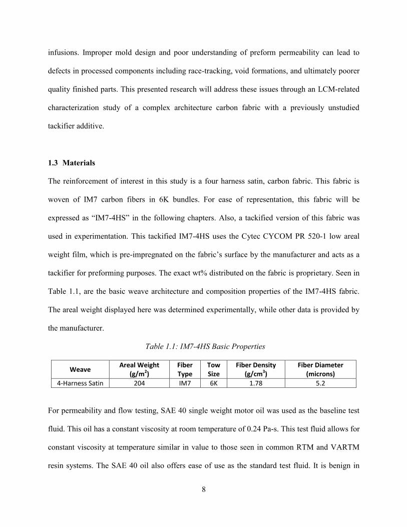
The reinforcement of interest in this study is a four harness satin, carbon fabric. This fabric is
woven of IM7 carbon fibers in 6K bundles. For ease of representation, this fabric will be
expressed as “IM7-4HS” in the following chapters. Also, a tackified version of this fabric was
used in experimentation. This tackified IM7-4HS uses the Cytec CYCOM PR 520-1 low areal
weight film, which is pre-impregnated on the fabric’s surface by the manufacturer and acts as a
tackifier for preforming purposes. The exact wt% distributed on the fabric is proprietary. Seen in
Table 1.1, are the basic weave architecture and composition properties of the IM7-4HS fabric.
The areal weight displayed here was determined experimentally, while other data is provided by
the manufacturer.
Table 1.1: IM7-4HS Basic Properties
Weave Areal Weight
(g/m2) Fiber Type
Tow Size
Fiber Density (g/cm3)
Fiber Diameter (microns)
4-Harness Satin 204 IM7 6K 1.78 5.2
For permeability and flow testing, SAE 40 single weight motor oil was used as the baseline test
fluid. This oil has a constant viscosity at room temperature of 0.24 Pa-s. This test fluid allows for
constant viscosity at temperature similar in value to those seen in common RTM and VARTM
resin systems. The SAE 40 oil also offers ease of use as the standard test fluid. It is benign in

9
relation to test equipment, whereas resins require extra cleanup time and preparation work so that
equipment is not destroyed. While investigating the effect of fluid type on permeability, a second
test fluid will be introduced: Applied Poleramic’s SC-15 epoxy resin. This resin will be
described in more detail in later chapters and is used in limited test settings.

10
2. Literature Review
For decades, researchers have studied liquid composite molding (LCM) processes and have
investigated the key process parameters and their resulting effects. Accurate and robust LCM
process modeling has been a continually sought goal in the field of advanced composite
manufacturing. Application of well-tuned process models allows for manufacturing optimization
and leads to better designed tooling and high quality finished composite parts. This present
research will overview LCM processes with a focus on Resin Transfer Molding (RTM) and go
further to survey the relevant work conducted on preform characterization including
compressibility and permeability for process modeling. These material parameters are of the
most important factors in creating an accurate LCM infusion model. Experimental techniques
will be discussed for both preform compressibility and permeability characterization. Modeling
approaches of empirical, analytical and numerical nature will also be surveyed for these
parameters.
11
2.1 Liquid Composite Molding
Liquid composite molding is a class of composite manufacturing that is generally applied to the
infusion of fibrous reinforcement with a thermosetting resin. In general, LCM processes consist
of injecting a resin into a dry bed of fiber reinforcement housed in a mold, which is then cured to
create a finished composite part. The LCM family of processes consists of multiple techniques.
Some of the most popular techniques include resin transfer molding (RTM), compression resin
transfer molding (CRTM), RTM light, vacuum-assisted resin transfer molding, (VARTM), resin
infusion (RI), structural injection molding (SRIM), resin film infusion (RFI), and Seemann
Composite Resin Infusion Molding Process (SCRIMP). These various techniques offer different
advantages depending on the application. RTM, a rigid closed mold technique, has found
application in the automotive and aerospace industries due to its potential for high production
rates and quality of finished parts [5]. RTM light possesses a similar setup to RTM but offers the
ability to visually observe the progress of the resin impregnation through translucent flexible
tooling. VARTM consists of vacuum-bagging the fiber reinforcement to a tool, which is
essentially an open mold process where a vacuum pump drives the resin infusion. The VARTM
process has been used produce medium to large, high performance composite parts, often in the
marine and aerospace industry, where the equipment cost is much lower than that of RTM [13].
In the SCRIMP method, channels are used in the tooling to reduce flow resistance during
infusions, which distribute the resin quickly across the part then wets out the preform [14]. The
SCRIMP technique is used to produce large composites such as boats or decks while offering a
safer alternative compared to the traditional hand lay-up or spray-up techniques used for those
products, which produce high volatile organic compound emissions [15]. This research will
focus on the RTM method, and further literature will be reviewed on this subset. Other LCM

12
techniques will not be discussed in detail here, but further background can be found in [14], [16],
[17].
Traditionally, optimization of composite manufacturing was an experience based and trial-and-
error approach, but in the last few decades, engineers have begun implementing process
modeling to mitigate manufacturing expenses [17]. The modeling of an LCM processes can
include reinforcement draping, impregnation, and curing. Of these aspects, understanding the
flow process is of utmost importance for all the liquid molding processes [14]. Poor
reinforcement saturation or fiber wet-out can produce low quality or unusable finished parts.
Using process modeling, simulations can be used to predict resin flow through the fiber
reinforcement and bring to light potential problem areas in the tooling or infusion. Based on
these simulation results, tooling, material, and process parameters can be optimized before any
high-cost decisions are made. LCM process parameters have been studied for decades and still
can present difficulties in manufacturing environments. Specifically, the RTM process and
parameters will be reviewed next.
2.1.1 Resin Transfer Molding
The basic RTM method involves injected a thermosetting resin into a dry fiber reinforcement
inside a closed mold. The mold is then heated to cure the matrix and opened to reveal a finished
composite part. RTM was first developed mainly for use in the aerospace sector, and has grown
to be a widely used method for composite manufacturing in not only aerospace, but also in the
automotive, civil, and sporting goods industries [14]. Now, RTM is considered the state-of-the-
art method for producing textile reinforced composite parts [18]. Although RTM processing has

13
been studied for many years, it is still considered to be underutilized, while reproducibility and
better understanding of the resin flow are considered to be the main obstacles holding this
technology back [14]. In a general sense, the RTM process can be split into three steps: fiber
preforming, resin infusion, and part curing.
2.1.1.1 Fiber Preforming
In RTM, the fiber reinforcement is often assembled outside of the mold into a preform, which is
in the shape of the finished part [8]. For complex shape composite parts, the fiber reinforcements
need to deform to the shape of the mold surface [19], thus a need for the dry reinforcement to
hold these contours is born. Here, preforming allows for easier handling of the reinforcement and
the ability to prepare for near net-shape production. The most common preforming techniques
involve the use of fabrics where a polymer binder/tackifier or stitching and embroidery
techniques are often employed to hold fiber orientation and multiple layers together [20]. For this
study, particular focus will be applied to the use of binders or tackifiers.
Tackifiers are most commonly thermoplastic or thermosetting resins that retain a solid structure
at room temperature but melt with applied heat. The advantage of these resins are that upon
cooling, resolidification allows the bonding of plies or tows into a consolidated preform [8].
Preforms then can be handled without the loss of fibers in a final-part form which can then be
infused in an LCM process. Methods of tackifier application utilize powder, liquid, veil or string
forms that are applied to the reinforcement at some point during the manufacturing process [8],
[21]. Tackifiers have been studied for their effect on preform springback [9], [22], effected
finished-part mechanical properties [21], [23], [24], and permeability and fiber wet-out [9]–[12].
14
While several studies exist, compared to other parameters involving permeability and resin flow,
the effect of tackifiers in RTM and other LCM processes has been investigated on a much
smaller scale. Due to the variety of different tackifier forms and concentrations, and the added
variation of pre-processing abilities with tackifiers, the resulting influence on resin flow is
inherently complex. A main focus of this study will aim to clarify and quantify the effect of a
specific tackifier on preform compaction and permeability.
2.1.1.2 Resin Infusion
The majority of this thesis will investigate preform parameters and their effects during the
infusion stage of the RTM process. In this step, resin is injected at pressure or flow rate into the
closed mold and infiltrates the preform. Major quality problems have stated to come from
unbalanced resin flow during the infusion step [25], and thus has become a significant area of
research. The mold filling stage of the RTM and LCM processes are critical in the development
of a quality finished composite part. Poor infusion or misunderstanding of preform permeability
may lead to defects including dry spotting or void formations and can be avoided with
appropriate prediction methods [26]. These are important considerations as the standard of US
aeronautics rejects parts that contain more than 2% of void defects [27].
To understand the resin infusion, one must first consider the general multiphase flow and
thermodynamics inherent to the process. On a general level, the infusion can be considered as
non-isothermal fluid flow through a porous media, which can be modeled on the basis of fluid
velocity, pressure and temperature into the media [14]. This can become a very complex problem
when considering heat transfer from the mold to the preform and resin. The heat transfer, fluid

15
flow, and resin cure reaction are all coupled and must be solved simultaneously. The governing
equations for this general approach will not be discussed in detail here; more background can be
found in [14]. For simplification purposes, most researchers apply an isothermal flow
assumption. This allows investigators to approach the fluid flow uncoupled from heat transfer
and resin cure kinetics and the permeating fluid can be considered constant in viscosity [6].
Regarding isothermal flow and with the assumption of low Reynolds number, resin flow through
fibrous preforms has generally been considered to be modeled as flow through porous media
governed by Darcy’s law seen in Equation 1.
𝑄 =
𝑆𝐴
µ
∆𝑃
𝐿 (1)
In this relationship, 𝑄 is the volumetric fluid flow rate, 𝐴 is the medium’s area normal to the
flow direction, µ is the fluid viscosity, 𝐿 is the medium length in direction of flow, ∆𝑃 is the
measured pressure drop across that length, and 𝑆 is the porous medium’s permeability.
Permeability is proportionality constant in this relation and describes the ease of flow through a
porous media with units of length squared. Preform permeability is the key parameter that drives
the flow in RTM [25]. Depending on the preform geometry, fiber content and flow direction,
permeability can vary on the order of magnitudes. Significant research has been made in
experimental and theoretical fronts to define permeability for fiber reinforcements. This study
will extend research further to investigate flow properties and permeability with reinforcement
treated with a novel tackifier. Further background and research trends will be surveyed regarding
preform permeability and flow in Section 2.3.
16
2.1.1.3 Curing
Ideally after the preform is completely saturated with resin, the RTM mold is heated in a specific
cycle to cure the composite part. Resin curing is usually sought to be inhibited during the
infusion stage in order to maintain a low resin viscosity for quick fiber wet out and allow for full
saturation before the resin gels [28]. For a general, coupled solution, a cure kinetic model can be
introduced as an auxiliary equation directly into the heat and mass balance equations, as well as
relating to the flow model by virtue of resin viscosity [29]. Again, this is complex and specific
integration of this method is described in more detail in [29]. By using the isothermal flow
assumption as discussed earlier, a simpler thermal model can be used to describe cure. This
assumption can be justified if the mold fill time is much shorter than the time required for the
cure to affect viscosity of the resin [6]. This is often the case and will be a basis assumption for
the work in this thesis. Although resin cure and kinetics are an important aspects of the RTM
process, this is outside the scope of this study.
2.2 Reinforcement Compaction/Compressibility
Inherent to LCM processes are the manufacturing steps of loading the reinforcement in a tool or
mold, closing the mold, infusing, and unloading the finished part. These loading and unloading
portions of the manufacturing process can apply compression to the preform or reinforcement.
For example, in the RTM the reinforcement is compressed by the closing of the mold, and with
VARTM, a vacuum bag and vacuum pressure applies a compressive force to the preform. Also,
debulking techniques may be applied in the preform process before infusion resulting in desired
deformations or reinforcement compaction. The amount of compression experienced by
reinforcement can be directly related to the fiber volume fraction and therefore is an essential
17
area of interest for LCM, as the fiber content will influence permeability and the resin infusion.
Also for RTM, to acquire a desired fiber volume fraction, the tooling must be able to supply and
withstand sufficient compressive force, while in VARTM, the vacuum pressure and
compressibility of the preform will govern the finished part thickness [30]. The relaxation or
spring-back of a reinforcement may also be relevant in certain the manufacturing situations,
which is a studied phenomenon and should not be overlooked. These considerations are
paramount to design of a good LCM process. Understanding of the compression behavior in a
preform leads to a better understanding towards local preform variations, mold design, and
ultimately leads to the production of better finished parts.
2.2.1 Defining Compressibility
Typically, the compression/compaction of a reinforcement can be quantified by relating the
applied pressure on the material to the resulting reinforcement thickness or fiber volume fraction.
As compaction pressure increases on a reinforcement, the thickness is generally seen to drop,
while also the fiber volume fraction increases. Chen et al. [31] reviewed previous experimental
compaction data [32] for woven fabrics and redefined four regimes existing on a typical
compressibility curve of thickness versus pressure based on the works of [32], [33]. The authors
first described a Regime 0 as an initial point where no pressure is applied to the reinforcement.
Regime 1 was described as a linear portion of the thickness/pressure curve where compaction is
initiated and slight pressure is produced. Regime 2 then was described as a nonlinear stage
where the reinforcement is compacted further and large voids in the fabric’s structure are filled
and the reinforcement deforms. The researchers explained that the total deformation in this
regime was due to both compression of the fibers and compression of the voids in the

18
architecture. Finally, Chen et al. [31] described Regime 3, a linear region of the curve where high
pressure is applied. This region exhibits deformation of the fibers only as the porosity has
reached a constant minimum. Reinforcements are also measured during unloading of supplied
compaction pressure. Often, the unloading of a sample will exhibit a hysteresis phenomenon
evident during compaction cycles as a fully unloaded reinforcement often will possess a higher
volume fraction than what it initially had before the loading cycle. This difference can be
attributed to fiber rearrangement, breakage and sliding during a cycle [34].
Another important consideration of reinforcement compressibility is the relaxation of the fiber
network. Dependent on the loading cycle, the reinforcement may experience a viscoelastic
recovery, permanent deformation, and/or elastic spring-back. Studying these phenomena has also
been the aim of many researchers in LCM. The presence of resin or a test fluid in a preform
during compaction also has been seen to influence compressibility and is of interest for certain
LCM applications.
Quantifying the compressibility of reinforcements has been of interest in LCM research for many
years. Experimental methods including empirical modeling have been used successfully by many
researchers. Investigators have also created theoretical models based on beam theory,
micromechanical structures, and consideration of the reinforcement during nonlinear elastic and
viscoelastic behavior [30].
19
2.2.2 Measurement Techniques
While some theoretical models for the compressibility of fibrous reinforcements have been
created, they are idealized for specific materials and non-robust so experimental characterization
of preform compaction under loading and unloading is commonly employed. A common
compaction experiment will include the loading and unloading of fibrous reinforcement in a
matched metal mold to empirically derive a relationship between loading/supplied pressure and
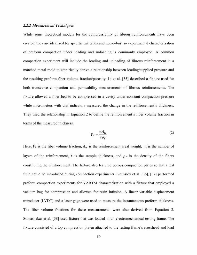
the resulting preform fiber volume fraction/porosity. Li et al. [35] described a fixture used for
both transverse compaction and permeability measurements of fibrous reinforcements. The
fixture allowed a fiber bed to be compressed in a cavity under constant compaction pressure
while micrometers with dial indicators measured the change in the reinforcement’s thickness.
They used the relationship in Equation 2 to define the reinforcement’s fiber volume fraction in
terms of the measured thickness.
𝑉𝑓 =
𝑛𝐴𝑤𝑡𝜌𝑓
(2)
Areal Weight Here, 𝑉𝑓 is the fiber volume fraction, 𝐴𝑤 is the reinforcement areal weight, 𝑛 is the number of
layers of the reinforcement, 𝑡 is the sample thickness, and 𝜌𝑓 is the density of the fibers
constituting the reinforcement. The fixture also featured porous compaction plates so that a test
fluid could be introduced during compaction experiments. Grimsley et al. [36], [37] performed
preform compaction experiments for VARTM characterization with a fixture that employed a
vacuum bag for compression and allowed for resin infusion. A linear variable displacement
transducer (LVDT) and a laser gage were used to measure the instantaneous preform thickness.
The fiber volume fractions for these measurements were also derived from Equation 2.
Somashekar et al. [38] used fixture that was loaded in an electromechanical testing frame. The
fixture consisted of a top compression platen attached to the testing frame’s crosshead and load
20
cell, while the material to be compacted was placed on a bottom platen. Laser gages were used to
measure the sample thickness during loading and unloading while a specified strain rate of
compaction was applied. The compaction study performed in this thesis reflects this method of
Somashekar et al. [38]. The details of which will be described in Chapter 3.
Additionally, the relaxation of a reinforcement may be studied using a similar setup to
compaction experiments. A typical relaxation experiment involves applying some type of
loading/unloading cycle or strain rate to a reinforcement sample, then stopping the load and
measuring the stress as a function of time as sample thickness is kept constant [39]. Somashekar
et al. [38] used their compaction fixture to investigate the viscoelastic recovery of reinforcements
through single compaction hold and quick release experiments and cyclical loading and
unloading experiments.
2.2.3 Empirical Models and Experimental Trends
To quantify the compaction of wool samples, Van Wyk [40] applied a power law model, seen in
Equation 3 based on beam theory, to empirically relate the applied stress, 𝜎, the fiber volume
fraction, 𝑉𝑓, and experimental constants 𝑎 and 𝑏.
𝜎 = 𝑎(𝑉𝑓)𝑏 (3)
Although this model is simplistic in nature and lacks certain physical and geometrical
consideration, it has been found to be successful spawning similar variations from following
researchers [30]. Batch et al. [41] used a heuristic method to describe the applied compaction
pressure in terms of the reinforcement’s spring constant, 𝐾, which is defined as a function of
fiber volume fraction, and 𝑉0 is the initial fiber volume fraction. This is seen in Equation 4.
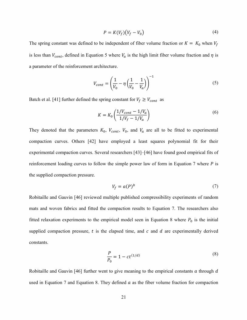
21
𝑃 = 𝐾(𝑉𝑓)(𝑉𝑓 − 𝑉0) (4)
The spring constant was defined to be independent of fiber volume fraction or 𝐾 = 𝐾0 when 𝑉𝑓
is less than 𝑉𝑐𝑜𝑛𝑡, defined in Equation 5 where 𝑉𝑎 is the high limit fiber volume fraction and 𝜂 is
a parameter of the reinforcement architecture.
𝑉𝑐𝑜𝑛𝑡 = (
1
𝑉0− 𝜂 (
1
𝑉0−1
𝑉𝑎))
−1
(5)
Batch et al. [41] further defined the spring constant for 𝑉𝑓 ≥ 𝑉𝑐𝑜𝑛𝑡 as
𝐾 = 𝐾0 (
1/𝑉𝑐𝑜𝑛𝑡 − 1/𝑉𝑎1/𝑉𝑓 − 1/𝑉𝑎
) (6)
They denoted that the parameters 𝐾0, 𝑉𝑐𝑜𝑛𝑡, 𝑉0, and 𝑉𝑎 are all to be fitted to experimental
compaction curves. Others [42] have employed a least squares polynomial fit for their
experimental compaction curves. Several researchers [43]–[46] have found good empirical fits of
reinforcement loading curves to follow the simple power law of form in Equation 7 where 𝑃 is
the supplied compaction pressure.
𝑉𝑓 = 𝑎(𝑃)𝑏 (7)
Robitaille and Gauvin [46] reviewed multiple published compressibility experiments of random
mats and woven fabrics and fitted the compaction results to Equation 7. The researchers also
fitted relaxation experiments to the empirical model seen in Equation 8 where 𝑃0 is the initial
supplied compaction pressure, 𝑡 is the elapsed time, and 𝑐 and 𝑑 are experimentally derived
constants.
𝑃
𝑃0= 1 − 𝑐𝑡(1/𝑑) (8)
Robitaille and Gauvin [46] further went to give meaning to the empirical constants 𝑎 through 𝑑
used in Equation 7 and Equation 8. They defined 𝑎 as the fiber volume fraction for compaction

22
pressure equal to 1 Pa (or essentially the initial fiber volume fraction), and 𝑏 was defined as the
compaction stiffening index, which is a value less than 1. For the relaxation model, 𝑐 was
defined as the pressure decay after 1 second, and 𝑑 was called the relaxation index. The authors
further defined a representative rigidity of the reinforcement, 𝑀, which was based on the linear
slope of a line passing through a low pressure point and the maximum compaction pressure
reached. The fiber volume fraction reached during each experiment was defined as the
representative fiber volume fraction or 𝑅𝑉𝑓. Using these parameters, the investigators made
several generalizations over the experimental results surveyed. As the number of plies in the
reinforcements increased, 𝑀 and 𝑎 were found to increase while 𝑏 decreased and 𝑅𝑉𝑓 decreased
for the oven materials. The compaction curves were seen to move progressively lower as the
fiber volume fraction reached 𝑅𝑉𝑓. Successive compaction cycles for the same sample were seen
to increase 𝑎 and 𝑅𝑉𝑓 while 𝑏 descreased. An increase in 𝑀 was also seen for woven fabrics in
this case. For relaxation experiments, less relaxation was seen as the applied pressure increased.
More relaxation was seen as the number of reinforcement plies or layers increased.
Regarding the observed hysteresis of loading/unloading cycles, in general, this phenomenon has
been found to be low for 2D fiber arrangements [34]. Although, significant hysteresis has been
found with compaction of glass fiber reinforcements [39] and in alumina preforms [47]. These
preforms of high compaction cycle hysteresis are stated by Michaud and Mortensen [34] to
possess fibers or binder material oriented along orthogonal to the testing axis. The researchers
also stated that there is no current model for reinforcement relaxation when hysteresis is
significant, and therefore phenomenological fitting is used.

23
Another important consideration during compaction experiments is the presence of a fluid. In
some debulking and LCM processes, the compaction of a resin saturated or partially saturated
preform may be relevant. This is especially pertinent to the VARTM process where first the
reinforcement experiences dry compaction, and then upon resin infiltration, a wetting
compaction and spring-back occur [36], [37]. To study this, researchers have performed wetted
compaction experiments. Under wetted conditions, the arrangement of the fibrous network is
altered due a lubricating effect from the wetting fluid and results in an increase of compaction
[36]. Robitaille and Gauvin [46] also noted this trend in their review of compaction experiments
as they noted the addition of a lubricant raises the representative fiber volume fraction (𝑅𝑉𝑓).
For the VARTM process or with the presence of resin in the reinforcement, the transverse
equilibrium inside the mold has been defined as the pressure balance seen in Equation 9 [36],
[37]. Here, 𝑃𝑎𝑡𝑚 is the applied atmospheric pressure, 𝑃𝑟 is the resin pressure, and 𝑃𝑓 is the
pressure supported by the fiber preform.
𝑃𝑎𝑡𝑚 = 𝑃𝑟 + 𝑃𝑓 (9)
Grimsley et al. [36], [37] used the relation in Equation 10 to define fiber volume fraction during
their VARTM compaction experiments in terms of the compressive strain rate, 𝜀, and the initial
reinforcement porosity, 𝜑0.
𝑉𝑓 =
1 − 𝜑01 − 𝜀
(10)
Initially in VARTM, the preform is compacted in a dry state by the vacuum pressure. Then resin
is injected and the local net pressure applied to the preform drops as described in Equation 9
[37]. With these physics of the VARTM process in mind, Grimsley et al. [36], [37] described the
compressive strain experienced by the preform with a dry loading compaction test fitted to the
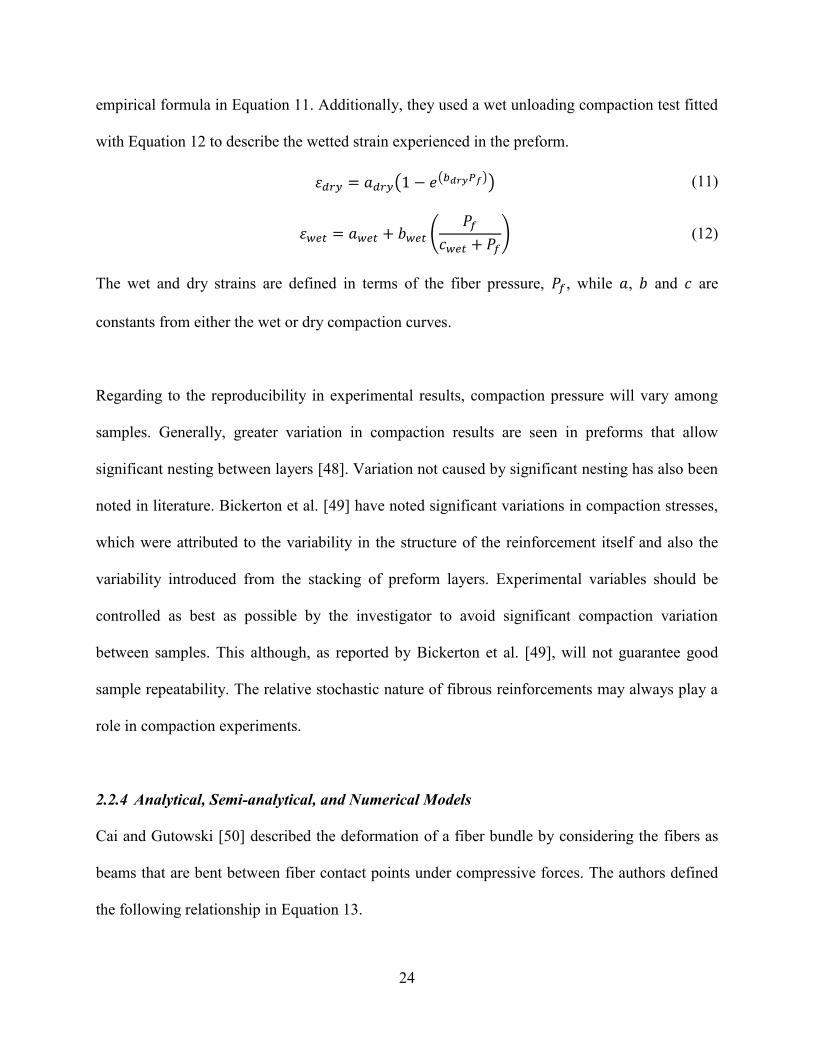
24
empirical formula in Equation 11. Additionally, they used a wet unloading compaction test fitted
with Equation 12 to describe the wetted strain experienced in the preform.
𝜀𝑑𝑟𝑦 = 𝑎𝑑𝑟𝑦(1 − 𝑒(𝑏𝑑𝑟𝑦𝑃𝑓)) (11)
𝜀𝑤𝑒𝑡 = 𝑎𝑤𝑒𝑡 + 𝑏𝑤𝑒𝑡 (
𝑃𝑓
𝑐𝑤𝑒𝑡 + 𝑃𝑓) (12)
The wet and dry strains are defined in terms of the fiber pressure, 𝑃𝑓, while 𝑎, 𝑏 and 𝑐 are
constants from either the wet or dry compaction curves.
Regarding to the reproducibility in experimental results, compaction pressure will vary among
samples. Generally, greater variation in compaction results are seen in preforms that allow
significant nesting between layers [48]. Variation not caused by significant nesting has also been
noted in literature. Bickerton et al. [49] have noted significant variations in compaction stresses,
which were attributed to the variability in the structure of the reinforcement itself and also the
variability introduced from the stacking of preform layers. Experimental variables should be
controlled as best as possible by the investigator to avoid significant compaction variation
between samples. This although, as reported by Bickerton et al. [49], will not guarantee good
sample repeatability. The relative stochastic nature of fibrous reinforcements may always play a
role in compaction experiments.
2.2.4 Analytical, Semi-analytical, and Numerical Models
Cai and Gutowski [50] described the deformation of a fiber bundle by considering the fibers as
beams that are bent between fiber contact points under compressive forces. The authors defined
the following relationship in Equation 13.
25
𝑃𝑓 =3𝜋𝐸
𝛽4
(1 −√𝑉𝑓𝑉0)
(√𝑉𝑎𝑉𝑓− 1)
4
(13)
Gutowski [50]
In this model, 𝐸 is the Young’s modulus of the fiber, 𝛽 is the span length-to-height ratio for the
fibers treated as beams, 𝑉0 is the initial fiber volume fraction, and 𝑉𝑎 is the maximum available
fiber volume fraction. This model has generally been applied semi-analytically to fit
experimental curves as the parameters 𝛽 and 𝑉𝑎 are difficult measure directly [35]. Toll et al.
[51], [52] employed micromechanical theory to develop a relationship of compaction pressure
and fiber volume fraction for fiber networks including a general 3D wad, a planar mat of
dispersed fibers, a bundle of parallel fibers and woven mats. Using statistical determination of
fiber contact points, power law relationships were developed for each configuration. Michaud
and Mortensen [34] summarized these relationships into the form seen in Equation 14.
𝑃𝑓 = 𝑘𝐸(𝑉𝑓 − 𝑉0)𝑛 (14)
In this equation, 𝑘 and 𝑛 are analytical parameters dependent on the arrangement of the fiber
network. Chen et al. [33], [53], [54] applied a unit cell approach to model compaction behavior
of woven fabrics. The researchers created analytical expressions for the idealized geometries
used. They concluded that their compaction models delivered good quantification of the preform
geometry allowing for better representation of the resin flow channels than their previous
models. Verpoest and Lomov [55] applied a robust approach where micromechanical models for
compaction were integrated with WiseTex, a software package that allows generation of the unit
cell internal geometries of woven, braided, knitted, and multi-axial multi-ply stitched non-crimp
fabrics (NCF). Lin et al. [56] used a similar unit cell geometrical software tool in TexGen, an

26
open source code developed at Nottingham University, to model fabric compression. The
researchers applied a finite element modeling technique with TexGen created geometry of a
plain weave fabric. They found that the model captured the fabric compression response
including material nonlinearities, yarn interactions, as well as hysteresis. Nguyen et al. [57] also
applied a meso-scale unit cell modeling approach using the finite element method for a woven
fabric. They created their unit cell geometry and meshes with software developed by Hivet and
Boisse [58]. With this computational setup, the investigators were able to carry out simulated
compaction tests with multiple layers of the woven fabric.
In recent years, numerical models for compaction have offered a much promise, incorporating
the detailed geometric consideration that analytic models lack. Numerical models are now
becoming more robust and moving towards a more ideal approach, where draping models
including preform compaction are now being coupled directly with resin infiltration models [20].
2.3 Reinforcement/Preform Permeability
2.3.1 Defining Permeability
2.3.1.1 Darcy’s Law
The most critical parameter of the RTM mold filling stage is the preform permeability [43].
Permeability describes the ease of fluid flow through a porous media. Henry Darcy [59] first
described the flow through a porous media by observing water flow through sand beds. He
concluded the following empirical relationship seen in Equation 15.
𝑄 =
𝑆𝐴
µ
∆𝑃
𝐿 (15)
27
Darcy’s law equates the volumetric flow rate of fluid, 𝑄, to a quantity of the permeability, 𝑆,
fluid viscosity, µ, cross-sectional area normal to the flow, 𝐴, and pressure difference, 𝛥𝑃, over a
length in the direction of flow, 𝐿. By dividing each side of the equation by the area, Darcy’s law
can also be expressed in the fashion seen in Equation 16.
𝑞 = −
1
µ[S]∇𝑃 (16)
Here, 𝑞 is the fluid superficial velocity, and ∇𝑃 is the pressure gradient, which is the pressure
difference over the length in the direction of flow. As discussed at the beginning of this review,
Darcy’s law has been widely accepted in the composite processing community to describe flow
through a fibrous reinforcement in LCM processes. Here, permeability is the key parameter of
units of meters squared. Permeability is function of the reinforcement geometry and fiber volume
fraction. The fiber volume fraction of the reinforcement or 𝑉𝑓 is directly related to the porosity or
𝜑 of the medium by the relationship seen in Equation 17.
𝜑 = 1 − 𝑉𝑓 (17)
In general, permeability decreases as fiber volume fraction of a fibrous reinforcement increases.
This relationship is well understood and has been reported in a review of experimental
permeability measurements [60]. Higher fiber volume fraction directly relates to less porous
zones for fluids to permeate, creating a greater pressure differential needed to overcome the
permeability. As for geometry, tightly woven fabrics are seen to have a lower permeability in
LCM processes than loosely woven/braided fabrics as resin has less porous zones and gaps to
more easily permeate. Defining this permeability parameter has been researched widely through
experimental and theoretical work for varying reinforcements and preforms.
28
Permeability is a tensor and a directional property depending on preform type. Preforms
composed of random fiber mats have been found to be isotropic in nature, where permeability is
found to be the same in all directions of the reinforcement [60]. For anisotropic preforms, a three
dimensional form of Darcy’s law must applied to describe the flow. This is seen in open form in
Equation 18.
{
𝑞𝑥𝑞𝑦𝑞𝑧} = −
1
µ[
𝑆𝑥𝑥 𝑆𝑥𝑦 𝑆𝑥𝑧𝑆𝑦𝑥 𝑆𝑦𝑦 𝑆𝑦𝑧𝑆𝑧𝑥 𝑆𝑧𝑦 𝑆𝑧𝑧
] [
𝜕𝑃/𝜕𝑥𝜕𝑃/𝜕𝑦𝜕𝑃/𝜕𝑧
] (18)
The x-, y- and z-directions are represented here where the x- and y-components represent the in-
plane directions and the z-direction is through the thickness. Often for directional fabric
reinforcements, the x-direction is defined to be parallel to the warp, and the y-direction is along
the weft/fill or 90° from the warp. The z-direction is then normal to the x-y plane. The
permeability tensor can be diagonalized by a coordinate transformation seen in Equation 19 to
produce a set of three principal permeabilities 𝑆11, 𝑆22, and 𝑆33 where 𝑇 is the transformation
matrix.
[
𝑆𝑥𝑥 𝑆𝑥𝑦 𝑆𝑥𝑧𝑆𝑦𝑥 𝑆𝑦𝑦 𝑆𝑦𝑧𝑆𝑧𝑥 𝑆𝑧𝑦 𝑆𝑧𝑧
] = [𝑇] [𝑆11 0 00 𝑆22 00 0 𝑆33
] [𝑇]𝑇 (19)
The principal permeabilities and their directions are often of interest for RTM modeling.
Generally, preforms can often be considered orthotropic in nature. For these orthotropic
preforms, three-dimensional Darcy’s law seen in Equation 18 will reduce to a one-dimensional
form for the x-, y- and z-directions [44]. These relations can be seen in Equation 20.
𝑞𝑥 = −
𝑆𝑥𝑥𝜇
𝑑𝑃
𝑑𝑥 (20a)

29
𝑞𝑦 = −
𝑆𝑦𝑦
𝜇
𝑑𝑃
𝑑𝑦 (20b)
𝑞𝑧 = −
𝑆𝑧𝑧𝜇
𝑑𝑃
𝑑𝑧 (20c)
With this formulation, a series of one-dimensional experiments are able to be carried out to
determine the permeability tensor of an orthotropic preform or reinforcement of interest. Using
the formulation in Equation 20, measurements can be made in the in-plane domain (x-y plane),
including an x-direction, y-direction and an off-axis measurement of 45° from the x-axis. This
allows a two-dimensional diagonalization of the permeability tensor to be performed resulting in
in-plane principal permeabilities 𝑆11 and 𝑆22 and their orientations, while a final measurement in
the z-direction will effectively produce the third principal permeability [45]. Considering two-
dimensional permeability or the in-plane directions only, the permeability tensor takes the form
seen in Equation 21.
[𝑆] = [
𝑆𝑥𝑥 𝑆𝑥𝑦𝑆𝑥𝑦 𝑆𝑦𝑦
] (21)
In this two-dimensional system, the permeability tensor components are related to two principal
in-plane permeabilities and a principal coordinate system, which can be seen in Equation 22
where 𝛽 is the angle between the first principal permeability and x- or warp axis [6].
𝑆𝑥𝑥 =
𝑆11 + 𝑆222
+𝑆11 − 𝑆22
2cos 2𝛽 (22a)
𝑆𝑥𝑦 =
𝑆11 − 𝑆222
sin 2𝛽 (22b)
𝑆𝑦𝑦 =
𝑆11 + 𝑆222
−𝑆11 − 𝑆22
2cos 2𝛽 (22c)

30
This angle 𝛽 is often of high interest in process modeling as it defines the orientation of principal
flow direction, and 90° to this angle is the second principal permeability or direction of highest
resistance to flow. This orientation angle can be observed in two-dimensional radial infusions of
preforms or it can be determined by a series of one dimensional channel flow experiments as
described by Fingerson [45] or by Weitzenböck [61]. Methods of this nature will be discussed in
more detail in the Measurement Techniques section.
Commonly in RTM, infusions are made parallel to the direction of the fabric preform, and parts
are relatively thin compared to their length. Due to this, resin flow is often assumed to be a two-
dimensional problem where in-plane permeabilities are dominant [6]. With thicker parts and
complex part geometry, transverse permeability plays a larger role in the description of the mold
fill and must be investigated. For this study, in-plane and transverse or through-thickness
permeabilities will be investigated for a more robust characterization of the reinforcements of
interest.
2.3.1.2 Assumptions
It should be noted that a Darcy’s law formulation for permeability is valid upon the assumption
of Newtonian fluid and creeping flow or a low Reynolds number [62]. Interpretation of the
Reynolds number for fibrous reinforcements varies depending on length scale and fabric type.
Engineering judgment must be used when defining the characteristic length used in the Reynolds
number calculation. Gauvin et al. [63] defined 𝑅𝑒 as the Reynolds number for continuous strand
mats with a characteristic length of 𝑑𝑓 or the roving diameter seen in Equation 23, where 𝜌 is the
fluid mass density, 𝜇 is the dynamic viscosity and 𝑣 is the flow velocity.
31
𝑅𝑒 =
𝜌𝑣𝑑𝑓
𝜇 (23)
Drapier et al. [64], in perhaps a more sensical approach, defined a maximum Reynolds number
for their studied biaxial stitched fabric in Equation 24.
𝑅𝑒𝑚𝑎𝑥 =
𝜌𝑣𝑚𝑎𝑥𝑑
𝜇 (24)
Here, 𝑣𝑚𝑎𝑥 is defined as the maximum fluid velocity encountered and 𝑑 is the largest
characteristic length defined as the largest stitching hole that was measured from micrographs of
the reinforcement. The authors were able to show a maximum Reynolds number that was far less
than 1. Shojaei et al. [65] defined Reynolds number using the square root of preform
permeability as the characteristic length in Equation 25.
𝑅𝑒 =
𝑣∗𝜌√𝑆
𝜇 (25)
Here, 𝑆 is the preform permeability and 𝑣∗ is the average particle velocity, which is related to the
Darcy velocity by the relationship
𝑣∗ =𝑣
𝜑 (26)
This relation uses the Darcy velocity, 𝑣, and the preform porosity, 𝜑, to define the average
particle velocity. The significance of non-Darcy flow will be investigated in Chapter 6, as high
flow rates or injections pressures have been used in industry during RTM applications and this
flow scenario may be applicable.
2.3.2 Measurement Techniques
There is no universally accepted, standard method for permeability measurements of LCM
reinforcements. Basic test methods use similar formulation to determine permeability, but have

32
many variants of fixture types and test parameters. Measurement of reinforcement permeability
is known to be notoriously variable in results where variation has been found to be up to an order
of magnitude between test methods for the same material [66]. Attempts have been made to
standardize methods for collaborative measurement studies where setup consistency and error
reduction is of main focus [66]–[69]. Other standardization efforts include a permeability
database creation [70], a proposed 3D woven reference fabric [71], and a proposed epoxy-based
reference test specimen not of fibrous architecture [18].
Of the myriad of measurement techniques employed to obtain the permeability parameter for
preforms used in resin infusion modeling, general formulation is based on Darcy’s law. At a
most basic level, these techniques generally fall in either 1D channel flow or 2D radial
measurement methods, while a few methods [72]–[76] have been developed to measure 3D
permeability tensor of a preform. One-dimensional methods involve linearly injecting a test fluid
(line-source to line-sink) into a preform placed in a rectangular cavity. Radial measurements are
conducted by centrally injecting a test fluid in a preform and observing the resulting propagation
of the flow front ellipse in the in-plane directions. Although other methods have also been used
to obtain permeability, this research will focus on linear injection and radial methods, as these
are most common and are used in this study. Other notable methods researchers have employed
include capillary rise techniques to find tow or fiber bundle permeability [77]–[79].
2.3.2.1 1D Linear Techniques
The basis of the 1D channel flow permeability measurement techniques is to isolate one direction
of a preform by a linear fluid injection to obtain one component of the permeability tensor. One-

33
dimensional flow experiments can be made in either a transient or steady-state case. There are
benefits and disadvantages to each case. Transient or advancing flow front methods involve a
measurement of an unsaturated permeability and reflect the transient nature seen an actual RTM
mold fill. Steady-state or saturated permeability methods are conducted after a preform has been
completely filled with test fluid. This is at a different physical state than seen in RTM mold fills,
but these saturated methods allow the ability to measure permeability at unlimited fiber volume
fractions or preform thicknesses with one sample, while transient techniques can only be tested
at a single fiber volume fraction [45]. In this respect, saturated methods allow a user to develop a
much larger range of data points for a preform than what could be done with an unsaturated
experiment on a sample/material amount basis. Methods and fixtures have also been developed
to allow an investigation on both unsaturated and saturated flow in a single test sample [11],
[45]. This is done by first measuring unsaturated permeability in a transient injection, then taking
steady state measurements at the same or higher fiber volume fraction of the original infusion.
In experimental measurements of saturated permeability, a constant flow rate injection is used to
permeate the preform and measurements are made after flow has reached a steady-state
condition. With this technique, saturated permeability 𝑆𝑠𝑎𝑡 can be determined using a Darcy’s
law formulation seen in Equation 27.
𝑆𝑠𝑎𝑡 =
𝑄𝜇𝐿
𝐴∆𝑃 (27)
This formulation is used for saturated 1D, in-plane permeability measurements, but also can be
used successfully in through-thickness or 𝑆𝑧𝑧 measurements with appropriately designed test
fixtures [44], [45]. In steady-state flow experiments, the volumetric flow rate, 𝑄 should have a
linear relationship with pressure drop across the preform. A researcher can obtain the saturated

34
permeability over a range of flow rates for a given fiber volume fraction. Any significant
nonlinearity seen in pressure versus flow rate curves during these investigations points to
possible test discrepancies of fixture leaking, progressive fiber displacement, or presence of
inertial effects.
For unsaturated flow methods, either a constant flow rate injection is used and the pressure drop
across the preform is measured, or a constant pressure injection is used and the flow front
position at a given time after initiation is measured. For 1D, transient or advancing front cases
Darcy’s law can be expressed on a temporal basis seen in Equation 28 where 𝑥(𝑡) represents the
flow front position (relative to the inlet) at time, 𝑡 [60].
𝑑𝑥
𝑑𝑡=
𝑆
𝜇𝜑
∆𝑃(𝑡)
𝑥(𝑡) (28)
Integrating this equation yields a solution for transient, unsaturated permeability, 𝑆𝑢𝑛𝑠𝑎𝑡, for
constant pressure injections seen in Equation 29 with initial condition of x(0) = 0 [60].
𝑆𝑢𝑛𝑠𝑎𝑡 =
𝑥2(𝑡)𝜇𝜑
2𝑡∆𝑃 (29)
This formulation is used for in-plane directions. Note that to measure a flow front position at a
given time, an unsaturated permeability fixture usually is implemented with a visualization
window and the infusion is recorded for analysis or the fixture is outfitted with in-cavity pressure
sensors along the flow path. At constant pressure injections, the flow front velocity slows with
increasing time and distance from inlet. To account for capillary effects, the capillary pressure
should be added to the pressure difference term used in Equation 29 [60]. If a constant flow rate
injection is used for measuring unsaturated permeability, the formulation seen in Equation 30
should be used.
35
𝑆𝑢𝑛𝑠𝑎𝑡 =
𝑄𝜇𝑥
𝐴∆𝑃 (30)
Here, 𝑥 represents the length at which the flow front has reached and ∆𝑃 is the instantaneous
pressure difference between the mold and atmospheric pressure. In constant flow rate, transient
experiments, the flow front position should be known for any time given the geometry of the
mold cavity, while the pressure varies with time and increasing flow front position.
2.3.2.2 2D Radial Technique
Radial permeability measurement techniques allow the in-plane permeabilities of a fabric to be
determined in a single infusion. Test fluid is injected at a circular inlet port at a central location
of a preform in a mold. The radially increasing flow front is then tracked over time in a transient
case. Generally, radial methods involve a fixture outfitted with a clear top or bottom so that the
flow front can be visually tracked, although some radial flow fixtures are designed with in-cavity
pressure transducers or sensors to evaluate flow front position [80]. For isotropic preforms, often
those of random fiber orientation, flow fronts advance in a circular shape as the permeability is
the same in all directions [60]. Weitzenböck et al. [81] defined the unsaturated radial
permeability, 𝑆𝑢𝑛𝑠𝑎𝑡 for isotropic reinforcements to be that seen in Equation 31 where t is the
time from initiation, 𝑟𝑓 is the radius of the flow front, and 𝑟0 is the radius of the inlet.
𝑆𝑢𝑛𝑠𝑎𝑡 =
𝜇𝜑
4𝑡∆𝑃{𝑟𝑓2[2 ln(𝑟𝑓/𝑟0) − 1] + 𝑟0
2} (31)
Weitzenböck et al. [81] also defined the unsaturated radial permeability for orthotropic materials
along both the x- and y- directions seen in Equation 32 and Equation 33 respectively. Here 𝑥𝑓
and 𝑦𝑓 are flow front position at time t of the each respective direction and 𝑥0 and 𝑦0 are the inlet
radii.
36
𝑆𝑥𝑥𝑢𝑛𝑠𝑎𝑡 =
𝜇𝜑
4𝑡∆𝑃{𝑥𝑓2[2 ln(𝑥𝑓/𝑥0) − 1] + 𝑥0
2} (32)
𝑆𝑦𝑦𝑢𝑛𝑠𝑎𝑡 =
𝜇𝜑
4𝑡∆𝑃{𝑦𝑓
2[2 ln(𝑦𝑓/𝑦0) − 1] + 𝑦02} (33)
When preparing preforms for radial permeability measurements, researchers have center hole-
punched their samples at the fixture inlet in order to eliminate any through thickness flow,
allowing for purely in-plane fluid propagation [67], [80]. This technique is advisable when using
reinforcements with low transverse permeability characteristics. Others have used a radial
technique that does not employ a center hole-punch and has the additional ability to measure
through-thickness permeability and in-plane flow to create a 3D measurement technique within a
single infusion [72].
2.3.3 Modeling and Prediction
Regarding theoretical permeability modeling, Lundström et al. [67] stated that “the theoretical
expressions that have been derived for the permeability are based on some specific and
simplified fiber arrangement and do not apply to a general case”. This fact continues to drive the
need for continuing experimental permeability measurement work and leaves a wanting for a
robust and adaptive permeability modeling tool. Several types of general models have been used
to characterize permeability for reinforcements: empirical, analytical, and numerical. These
models are often used to describe preform permeability as a function of fiber volume fraction
and geometry. While empirical models may present the most accurate and representative values,
they are based on time-consuming experimental characterization. Analytical and semi-analytical
models offer a reduction in experimentation but are often too idealized for application to
complex geometry preforms. Numerical permeability prediction has gained capability in recent

37
years and looks to be a promising future alternative to experimental measurements, although
added complexity to the numerical simulations can become computationally costly.
2.3.3.1 Empirical Models
Often, it is useful to model experimentally produced permeability over a range of fiber volume
fractions. If a suitable fit is found for a range measured permeabilities at several points of fiber
volume fraction, an accurate prediction of permeability can be extrapolated at fiber volume
fractions that were not tested with the specific preform. Multiple relations have been used to
model empirical trends in permeability throughout LCM research. A generalized version of the
Carman-Kozeny equation, seen in Equation 34, has been applied by many researchers to fit their
permeability measurements over a range of fiber volume fractions where 𝑎 and 𝑏 are constants
[6].
𝑆 =
𝑎(1 − 𝑉𝑓)𝑏+1
𝑉𝑓𝑏 (34)
Kim et al. [82] proposed a model of form in Equation 35 where 𝑉𝑓∞ is the fiber volume fraction
at maximum compression and the model is valid when 𝑉𝑓 ≤ 𝑉𝑓∞ and when 1 ≤ 𝑏 ≤ 1/𝑉𝑓∞.
𝑆 = 𝑎(𝑏𝑉𝑓∞ − 𝑉𝑓)
4 (35)
Gauvin et al. [63] developed the empirical model seen in Equation 36 for continuous strand mats,
where 𝑎, 𝑏, and 𝑐 are constants and 𝜑 is the mat porosity.
𝑆 = 𝑎 + 𝑏𝑒(𝑐𝜑) (36)
Tuncol [44] found good empirical fits for the fiber volume fraction range tested using a similar
exponential model in Equation 37.
38
𝑆 = 𝑎𝑒(𝑏𝑉𝑓) (37)
Several other researchers [36], [37], [43], [45], [83], [84] have found an appropriate fit using a
power law regression, seen in Equation 38, over a range of reinforcements.
𝑆 = 𝑎(𝑉𝑓)
𝑏 (38)
Overall, any empirical model can be justified to describe permeability if a good fit is resultant.
2.3.3.2 Semi-analytical and Analytic Models
Analytical and semi-analytical models for permeability prediction have been of interest in the
LCM community for decades. The ability to reduce experimental preform characterization or to
eliminate it entirely has great time and resource saving potential for LCM process modeling.
Researchers have employed method to predict permeability simply from the geometry of the
reinforcement alone using the lubrication approach. Due to the complexities of reinforcement
architectures and the dependence of permeability on geometry, accurate analytical prediction
different reinforcement types can be a difficult.
Many researchers have employed the Carmen-Kozeny equation to predict permeability for
unidirectional reinforcements [6]. While the relation was originally used for flow through
isotropic media composed of spherical particles, a modified version is used to describe flow
through a cylinder bed representative of aligned fibers [7]. This modified version of the Carman-
Kozeny relation defines permeability in Equation 39.
𝑆 =
𝑟𝑓2
4𝐶𝑘
(1 − 𝑉𝑓)3
𝑉𝑓2 (39)
39
Here, 𝑟𝑓 is the fiber radius, 𝐶𝑘 is the Kozeny constant, and 𝑉𝑓 is the fiber volume fraction. The
Kozeny constant then has to be determined and possesses different values for flow parallel and
perpendicular to the fiber bed. This relation was modified by Gutowski et al. [85] to account for
that fact that the Carman-Kozeny equation predicts a non-zero permeability at fiber volume
fractions higher than the theoretical maximum [7]. Gutowski et al. [85] proposed the following
modification for transverse permeability in Equation 40.
𝑆 =𝑟𝑓2
4𝐶𝑘′
(√𝑉𝑎′𝑉𝑓− 1)
3
(𝑉𝑎′𝑉𝑓+ 1)
(40)
In this equation, 𝐶𝑘′ and 𝑉𝑎′ are empirical parameters where 𝑉𝑎′ is the maximum available fiber
volume fraction. Later, Gebart [86] proposed that both the Carman-Kozeny equation and the
model from Gutowski et al. [85] lacked in detailed geometric consideration and could be
improved upon. Gebart [86] introduced the geometries of quadratic and hexagonal fiber packing
arrangements into a model for unidirectional permeability. Permeabilities parallel and
perpendicular to the fiber bed then were defined for quadratic and hexagonal fiber packing as
seen in Equation 41 and Equation 42.
𝑆∥ =
8𝑟𝑓2
𝐶∥(1 − 𝑉𝑓
𝑉𝑓2 )
3
(41)
𝑆⊥ = 𝐶⊥ (√𝑉𝑓𝑚𝑎𝑥
𝑉𝑓− 1)
5/2
𝑟𝑓2 (42)
Here, the maximum fiber volume fraction, 𝑉𝑓𝑚𝑎𝑥, constant 𝐶∥ and constant 𝐶⊥ are defined by
fiber packing arrangement in Table 2.1.
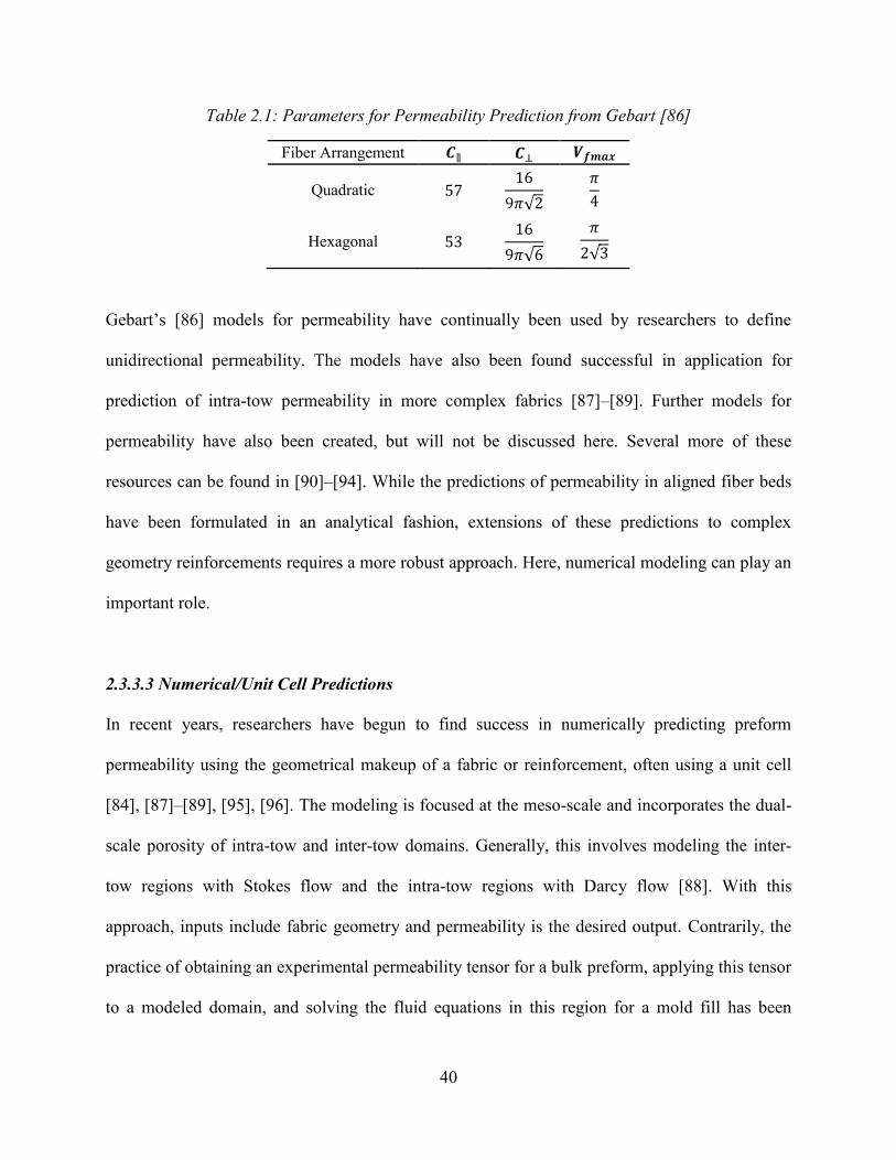
40
Table 2.1: Parameters for Permeability Prediction from Gebart [86]
Fiber Arrangement 𝑪∥ 𝑪⊥ 𝑽𝒇𝒎𝒂𝒙
Quadratic 57 16
9𝜋√2
𝜋
4
Hexagonal 53 16
9𝜋√6
𝜋
2√3
Gebart’s [86] models for permeability have continually been used by researchers to define
unidirectional permeability. The models have also been found successful in application for
prediction of intra-tow permeability in more complex fabrics [87]–[89]. Further models for
permeability have also been created, but will not be discussed here. Several more of these
resources can be found in [90]–[94]. While the predictions of permeability in aligned fiber beds
have been formulated in an analytical fashion, extensions of these predictions to complex
geometry reinforcements requires a more robust approach. Here, numerical modeling can play an
important role.
2.3.3.3 Numerical/Unit Cell Predictions
In recent years, researchers have begun to find success in numerically predicting preform
permeability using the geometrical makeup of a fabric or reinforcement, often using a unit cell
[84], [87]–[89], [95], [96]. The modeling is focused at the meso-scale and incorporates the dual-
scale porosity of intra-tow and inter-tow domains. Generally, this involves modeling the inter-
tow regions with Stokes flow and the intra-tow regions with Darcy flow [88]. With this
approach, inputs include fabric geometry and permeability is the desired output. Contrarily, the
practice of obtaining an experimental permeability tensor for a bulk preform, applying this tensor
to a modeled domain, and solving the fluid equations in this region for a mold fill has been

41
commonplace in LCM research for many years. The details of this modeling approach, including
resin cure kinetics and thermodynamic considerations, will not be discussed in this work. Further
background in this area can be found in [29], [97]. Permeability prediction with a unit cell aims
to reduce or eliminate the time consuming experimental characterization step of this numerical
modeling process.
Zeng et al. [87] used a numerical unit cell approach to predict permeability of the 2x2 twill
weave carbon fabric that was widely characterized in an international benchmark study [66],
[69]. They first geometrically characterized 9 layers of the fabric using x-ray micro-computed
Tomography (µ-CT). These tow and architecture geometries were then used as inputs into the
open source TexGen software developed from the University of Nottingham, which created a
representative unit cell. The tows were treated as porous media and Gebart’s [86] analytical
relations were used to define intra-tow permeability. The resulting intra-tow permeabilities were
deemed low enough to assume tow impermeability. Multiple simulated infusions were then run
on the modeled geometry in a computational fluid dynamics (CFD) package. The researchers
also incorporated nesting possibilities into their simulations using a Latin hypercube sampling
technique. It was concluded that, given accurate geometrical data, numerically predicted
permeability could be more reliable than the experimental data produced in the first round of the
benchmark exercise. Luchini et al. [84] used a similar approach to predict permeability in plain
weave glass fabric. Fabric geometry was measured from optical microscopy of a finished
composite laminate. This procedure took laminate measurements at the tow and intra-tow level.
The intra-tow geometry consisting of a fiber packing arrangement, fiber volume fraction, and
fiber diameter was characterized. Gebart’s [86] analytical expression was also used to find the
42
intra-tow permeability, and a representative unit cell was created in TexGen. Tows were treated
as porous media using the predicted intra-tow permeability and gaps between tows were handled
with Stokes flow. CFD simulations were run to produce a unit cell permeability, which compared
very well to experimental saturated permeability measurements of the same fabric in both the
warp and weft directions.
Tan et al. [89] compared similar CFD permeability predictions of small and large representative
unit cells of a biaxial stitched mat to experimental permeability. They also used Gebart’s [86]
analytical permeability for tow permeability and applied an finite element method (FEM)
approach to solve the fluid equations. It was found that the large unit cells over predicted
permeability, while the small unit cells under predicted the permeability compared to the
experimental results. Even with these results, the researchers stood by their conclusion that unit
cell numerical modeling is still an effective method for permeability prediction. Chen et al. [88]
also used a similar unit cell method and found acceptable agreement between numerical and
published experimental permeability results for several plain weave fabrics.
2.3.4 Other Factors of Consideration
2.3.4.1 Reinforcement Architecture/Fabric Type
Geometry and fiber volume fraction/porosity are the dominant factors affecting the permeability
of fibrous reinforcements. Being that there are many different types of complex fiber architecture
used to create preforms, the reported values of permeability vary greatly among reinforcement
types. Among those types include random fiber mats, unidirectional, woven, braided, stitched,
knitted and other architectures. These architecture types offer a wide scatter of potential resin
43
flow paths, which inherently affects the preform permeability. Also, a different fiber network
may be used in the same architecture being carbon, glass or other fiber types, which can further
create more possibility for permeability variation. Notably, preforms of natural fibers have been
reported to swell upon saturation, reducing porosity and affectively increasing flow resistance
[98]. Also, preforms featuring multiple fiber types (e.g. carbon and glass) can create further
variability.
As preform geometry as a major consideration, researchers have been able to prescribe some
generalities for permeability and flow behavior based on architecture. While random fiber mats
are known to be homogeneous in permeability, the presence of tows and gaps between tows in
woven fabrics create a heterogeneous medium [99]. Unidirectional reinforcements have been
seen to possess a higher permeability in the flow direction parallel to the fibers than that in the
perpendicular direction. This relationship has also been observed in Gebart’s [86] model for
unidirectional reinforcements. Endruweit and Long [100] investigated the in-plane principal
permeabilities of triaxial braided carbon fabrics with differing fiber bias angles (angles from the
warp axis or 0° line to the bias tow) at 45°, 60°, and 70°. With experimental data and numerical
modeling, the authors presented permeability as a function of triaxial fabric tow bias angle. It
was suggested that the first principal permeability was at 𝛽 = 0° for triaxial fabrics with bias
fibers up to approximately 55°. With bias fibers greater than 55°, the first principal permeability
was seen to shift from 𝛽 = 0° to 𝛽 = 90°. This result offers valuable insight for principal flow
direction of triaxial fabrics and similar investigations could be applied to other braided fabrics,
such as biaxial configurations. Permeabilities for other multiple fabric types are summarized in
[60] by preform direction (𝑆𝑥𝑥 and 𝑆𝑦𝑦). Regarding local preform directions, generally the
44
transverse or through-thickness permeability is seen to be lower than that of the in-plane
directions for most reinforcements [60]. Transverse permeability has been reported to be over
two magnitudes lower than the in-plane permeabilities of the same preform [101]. Aside from
any previously accepted generalization, understanding how fluid will flow through a specific
reinforcement cannot be confidently known without first employing experimental
characterization or robust modeling and simulation.
2.3.4.2 Wettability, Fluid and Capillary Effects
The effect of test fluid on experimental permeability measurements has been something of
debate in LCM preform characterization. A variety of test fluids have been used in permeability
experimentation throughout literature in lieu of actual thermosetting resins for reasons likely of
cost and ease of use where presence of similar rheological properties may be found in the
alternative fluid. Corn syrup [102]–[104] has commonly been used in experimental permeability
measurements, as have mixtures of corn syrup, water, and dye [105]–[107]. Previous research
has also justified the use of corn oil [82], hydraulic fluid [108], [109], silicon oil [110], [111],
and motor oil [112] in various experimental scenarios. Other notable works have used gaseous
fluids for permeability measurements including air [113], [114]. A study by Hammond and Loos
[115] concluded that fluid type had little effect on steady-state and advancing front permeability
while comparing corn oil, water and EPON 815 resin. Luo et al. [116] also concluded that fluid
type had an insignificant effect on permeability compared to the experimental variation when
comparing advancing front measurements made with silicone oil and diluted corn syrup.
Contrarily, Steenkamer et al. [117] saw large variations in measured permeability with different
test fluids of motor oil, diluted corn syrup and vinyl ester resin, and concluded that reinforcement
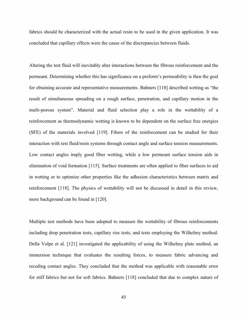
45
fabrics should be characterized with the actual resin to be used in the given application. It was
concluded that capillary effects were the cause of the discrepancies between fluids.
Altering the test fluid will inevitably alter interactions between the fibrous reinforcement and the
permeant. Determining whether this has significance on a preform’s permeability is then the goal
for obtaining accurate and representative measurements. Bahners [118] described wetting as “the
result of simultaneous spreading on a rough surface, penetration, and capillary motion in the
multi-porous system”. Material and fluid selection play a role in the wettability of a
reinforcement as thermodynamic wetting is known to be dependent on the surface free energies
(SFE) of the materials involved [119]. Fibers of the reinforcement can be studied for their
interaction with test fluid/resin systems through contact angle and surface tension measurements.
Low contact angles imply good fiber wetting, while a low permeant surface tension aids in
elimination of void formation [115]. Surface treatments are often applied to fiber surfaces to aid
in wetting or to optimize other properties like the adhesion characteristics between matrix and
reinforcement [118]. The physics of wettability will not be discussed in detail in this review,
more background can be found in [120].
Multiple test methods have been adopted to measure the wettability of fibrous reinforcements
including drop penetration tests, capillary rise tests, and tests employing the Wilhelmy method.
Della Volpe et al. [121] investigated the applicability of using the Wilhelmy plate method, an
immersion technique that evaluates the resulting forces, to measure fabric advancing and
receding contact angles. They concluded that the method was applicable with reasonable error
for stiff fabrics but not for soft fabrics. Bahners [118] concluded that due to complex nature of
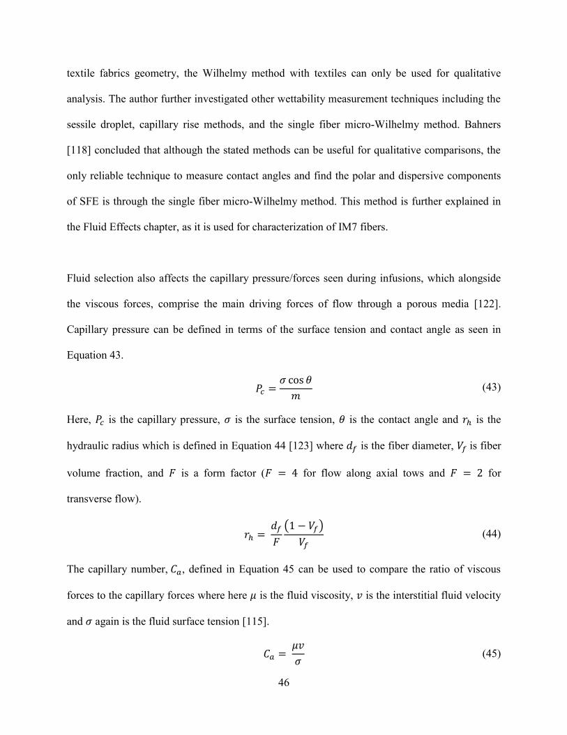
46
textile fabrics geometry, the Wilhelmy method with textiles can only be used for qualitative
analysis. The author further investigated other wettability measurement techniques including the
sessile droplet, capillary rise methods, and the single fiber micro-Wilhelmy method. Bahners
[118] concluded that although the stated methods can be useful for qualitative comparisons, the
only reliable technique to measure contact angles and find the polar and dispersive components
of SFE is through the single fiber micro-Wilhelmy method. This method is further explained in
the Fluid Effects chapter, as it is used for characterization of IM7 fibers.
Fluid selection also affects the capillary pressure/forces seen during infusions, which alongside
the viscous forces, comprise the main driving forces of flow through a porous media [122].
Capillary pressure can be defined in terms of the surface tension and contact angle as seen in
Equation 43.
𝑃𝑐 =
𝜎 cos 𝜃
𝑚 (43)
Here, 𝑃𝑐 is the capillary pressure, 𝜎 is the surface tension, 𝜃 is the contact angle and 𝑟ℎ is the
hydraulic radius which is defined in Equation 44 [123] where 𝑑𝑓 is the fiber diameter, 𝑉𝑓 is fiber
volume fraction, and 𝐹 is a form factor (𝐹 = 4 for flow along axial tows and 𝐹 = 2 for
transverse flow).
𝑟ℎ =
𝑑𝑓
𝐹
(1 − 𝑉𝑓)
𝑉𝑓 (44)
The capillary number, 𝐶𝑎, defined in Equation 45 can be used to compare the ratio of viscous
forces to the capillary forces where here 𝜇 is the fluid viscosity, 𝑣 is the interstitial fluid velocity
and 𝜎 again is the fluid surface tension [115].
𝐶𝑎 =
𝜇𝑣
𝜎 (45)

47
Advancing front or unsaturated permeability can be compared versus the capillary number, thus
displaying if permeability has dependence for a given range of produced data. Permeability was
found to be independent of capillary number by Hammond et al. [43] for their tests.. Amico and
Lekakou [124] and Lou et al. [116] both stated for injections pressures greater than 1 bar, the
capillary effect of capillary pressure on permeability is insignificant and can be neglected.
2.3.4.3 Dual-scale Porosity
Complex fiber reinforcements often can be said to possess dual-scale porosity; a porous zone is
defined at the tow level where gaps exist between the weave or braid of the tows, while the tows
themselves are porous, composed of a cluster of individual fibers. Researchers observed
behaviors of this dual scale porosity through comparisons of infusions with randomly aligned
and directional fiber preforms. Parseval et al. [125] found that while plotting transient inlet
pressure for a constant flow rate infusion, instead of seeing a linear increase of pressure as
predicted by Darcy’s law (and also seen in random fiber mat infusions), the resulting pressure
curved drooped for directional fabrics. This relationship is reproduced graphically in Figure 2.1.
Figure 2.1: Pressure Drooping Effect
Time
Inle
t P
ress
ure
Random fiber mat
Directional mat

48
Pillai and Advani [126] attributed this drooping effect to the dual scale porous nature of
directional fabrics where the permeating fluid first fills the gaps between tows, then lagging tow
saturation is seen behind the advancing flow front. They also developed a model that accurately
corrected for this pressure drooping by introducing a sink term to the continuity equation as seen
in Equation 46, which was substituted directly into Darcy’s law.
∇ ∙ 𝒗 = −𝛼𝑠 (46)
Here, v is the volume averaged velocity and 𝛼𝑠 is the sink term, which the researchers defined as
the volumetric rate of liquid absorption. Recently, the sink term has been further employed by
researchers to describe the phenomena characteristic of dual-scale porous media in LCM [127]–
[129].
Pillai [99] defined a dual-scale fabric by a comparison of characteristic lengths. By comparing
the length between tows, 𝐿𝑡𝑜𝑤, and the length between fibers within a tow, 𝑙𝑡𝑜𝑤, a dual-scale
fabric for LCM considerations will exhibit a relationship of 𝐿𝑡𝑜𝑤 ≫ 𝑙𝑡𝑜𝑤 . If both characteristic
lengths are of similar magnitude, the medium can be considered to possess a single scale of
porosity (e.g. a random fiber mat). A later experimental study by Babu and Pillai [130]
investigated multiple directional fabrics architectures for inlet pressure drooping and concluded
some directional fabrics did not exhibit drooping pressure curves. The authors hypothesized that
for a fabric to be considered dual-scale in nature, it then must possess “continuous uninterrupted
macro-channels”. It is clear that reinforcements of interest should be characterized carefully
before applying different models for resin flow and generalizations over entire fabric types.

49
Dependent on the geometry and fiber volume fraction, the fabric reinforcement of interest may
or may not possess a significant state of dual scale porosity.
Due to the transient saturation this dual scale model involves, it can be stated that in steady-state
flow scenarios, the permeability will not be affected by this dual scale nature in the same way.
Steady-state permeability measurements take place after a fabric reinforcement is fully saturated
with fluid. Thus, one would assume that Darcy’s law in conjunction with continuity without a
sink term would be sufficient to describe this flow, as no lagging saturation will be present. The
difference between advancing front and saturated permeability then must be explored.
2.3.4.4 State of Saturation
Steady-state and advancing front permeability measurement techniques involve different flow
considerations in porous media, and because of this, there has been much research regarding
saturated versus unsaturated permeability in LCM [65], [67], [71], [98], [125], [131]–[136].
Mold fills will naturally occur in an advancing front flow. Due to this, any difference between
permeability measurements made at a steady-state or in transient fill should be investigated. One
might consider that because of the differences between saturated and unsaturated flow through
porous media, advancing front permeability measurements should take priority over steady-state
measurements. Although, the benefit of creating permeability values at a full range of fiber
volume fractions from a single steady-state sample is attractive for reinforcement
characterization. By comparison, unsaturated measurements involve a process of testing a single
sample per volume fraction point of interest, which can lead to large material consumption and
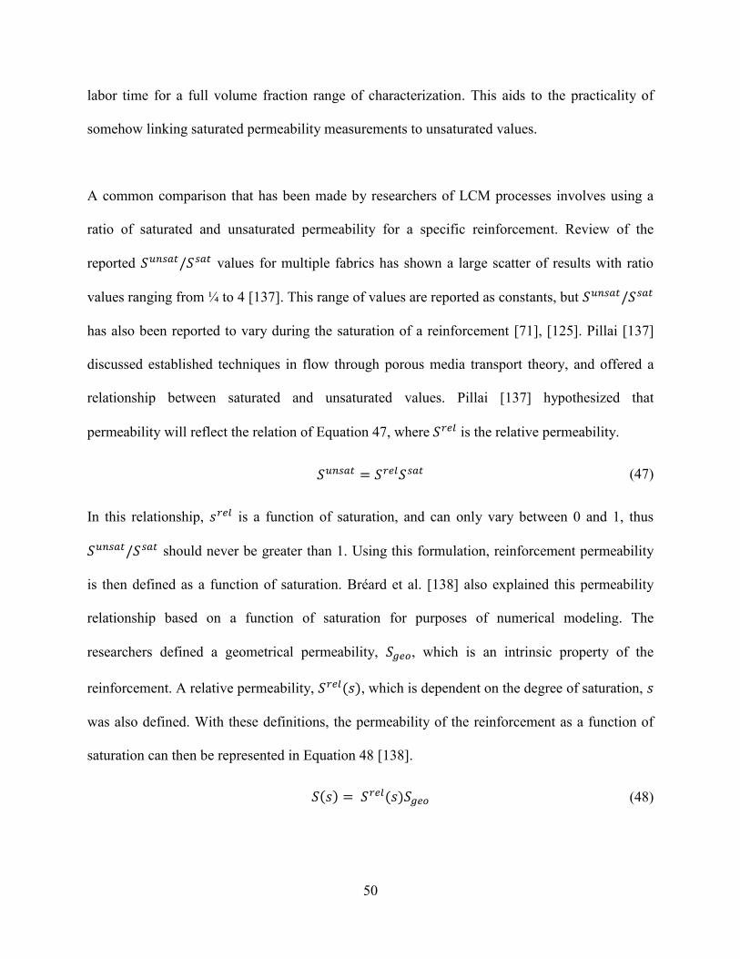
50
labor time for a full volume fraction range of characterization. This aids to the practicality of
somehow linking saturated permeability measurements to unsaturated values.
A common comparison that has been made by researchers of LCM processes involves using a
ratio of saturated and unsaturated permeability for a specific reinforcement. Review of the
reported 𝑆𝑢𝑛𝑠𝑎𝑡/𝑆𝑠𝑎𝑡 values for multiple fabrics has shown a large scatter of results with ratio
values ranging from ¼ to 4 [137]. This range of values are reported as constants, but 𝑆𝑢𝑛𝑠𝑎𝑡/𝑆𝑠𝑎𝑡
has also been reported to vary during the saturation of a reinforcement [71], [125]. Pillai [137]
discussed established techniques in flow through porous media transport theory, and offered a
relationship between saturated and unsaturated values. Pillai [137] hypothesized that
permeability will reflect the relation of Equation 47, where 𝑆𝑟𝑒𝑙 is the relative permeability.
𝑆𝑢𝑛𝑠𝑎𝑡 = 𝑆𝑟𝑒𝑙𝑆𝑠𝑎𝑡 (47)
In this relationship, 𝑠𝑟𝑒𝑙 is a function of saturation, and can only vary between 0 and 1, thus
𝑆𝑢𝑛𝑠𝑎𝑡/𝑆𝑠𝑎𝑡 should never be greater than 1. Using this formulation, reinforcement permeability
is then defined as a function of saturation. Bréard et al. [138] also explained this permeability
relationship based on a function of saturation for purposes of numerical modeling. The
researchers defined a geometrical permeability, 𝑆𝑔𝑒𝑜, which is an intrinsic property of the
reinforcement. A relative permeability, 𝑆𝑟𝑒𝑙(𝑠), which is dependent on the degree of saturation, 𝑠
was also defined. With these definitions, the permeability of the reinforcement as a function of
saturation can then be represented in Equation 48 [138].
𝑆(𝑠) = 𝑆𝑟𝑒𝑙(𝑠)𝑆𝑔𝑒𝑜 (48)
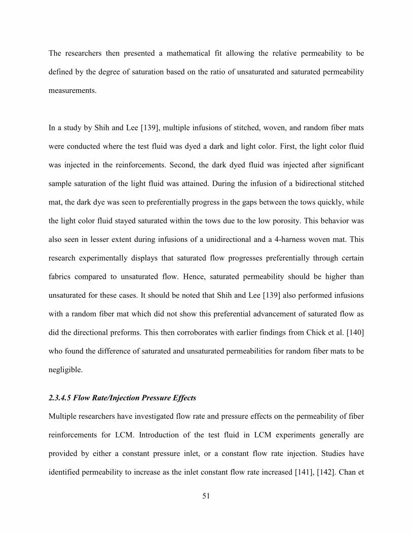
51
The researchers then presented a mathematical fit allowing the relative permeability to be
defined by the degree of saturation based on the ratio of unsaturated and saturated permeability
measurements.
In a study by Shih and Lee [139], multiple infusions of stitched, woven, and random fiber mats
were conducted where the test fluid was dyed a dark and light color. First, the light color fluid
was injected in the reinforcements. Second, the dark dyed fluid was injected after significant
sample saturation of the light fluid was attained. During the infusion of a bidirectional stitched
mat, the dark dye was seen to preferentially progress in the gaps between the tows quickly, while
the light color fluid stayed saturated within the tows due to the low porosity. This behavior was
also seen in lesser extent during infusions of a unidirectional and a 4-harness woven mat. This
research experimentally displays that saturated flow progresses preferentially through certain
fabrics compared to unsaturated flow. Hence, saturated permeability should be higher than
unsaturated for these cases. It should be noted that Shih and Lee [139] also performed infusions
with a random fiber mat which did not show this preferential advancement of saturated flow as
did the directional preforms. This then corroborates with earlier findings from Chick et al. [140]
who found the difference of saturated and unsaturated permeabilities for random fiber mats to be
negligible.
2.3.4.5 Flow Rate/Injection Pressure Effects
Multiple researchers have investigated flow rate and pressure effects on the permeability of fiber
reinforcements for LCM. Introduction of the test fluid in LCM experiments generally are
provided by either a constant pressure inlet, or a constant flow rate injection. Studies have
identified permeability to increase as the inlet constant flow rate increased [141], [142]. Chan et
52
al. [141] explained this behavior through a phenomenon of “preferential channeling” where the
fluid is pushed through the larger gaps in the reinforcement geometry, avoiding the lower
porosity areas as the pressure builds. The authors further added that this preferential channeling
may lead to tows not being fully saturated during infusions. Trevino et al. [143] also described a
channeling effect while testing directional fiber mats, but noted that it was observed for low fiber
volume fractions, below 35% when the preform was not tightly packed. High pressure build ups
were not seen until fiber volume fraction was higher than 55%. In comparison, Chen et al. [141]
and Young et al. [142] saw increasing of permeability with flow rate while using preforms
compacted to 44.8% fiber volume fraction, and lower 30% fiber volume fraction, respectively.
These results point to the significance of fiber volume fraction. Significant research in high fiber
volume fraction ranges (those at 55% and higher, often of interest in aerospace applications) has
not been investigated in this area.
Other researchers have found permeability to be independent of the tested ranges of constant
inlet pressures injections [65], [67], [144]. Lundström et al. [67] reported constant permeability
over a tested pressure range of 0.5 to 1.5 bars. Kim et al. [144] also corroborated similar results
for a pressure range of 1.5 to 2 bars. Shojaei et al. [65] explained that the permeability remained
independent over a range of 1 to 3 bars because at those selected pressures, the critical flow rate
for the woven E-glass fabric was not achieved at which non-Darcy flow appears. The authors
observed this critical fluid velocity to be around 0.2 cm/s through experimental work for their
specific fabric type and fiber volume fraction. Also, as stated earlier, with pressure inlet
injections made under 1 bar, capillary effects may be significant and permeability could be
affected differently at these low pressures [116], [124].
53
This research involving critical flow rates/velocities for constant permeability or Darcy flow can
become of interest when researching high flow rate or velocity flows in LCM. Although most
flow in LCM are described to be of low Reynolds number or creeping flow, possibilities of non-
Darcy behavior at high flow rates or pressures in industrial is applicable. Forchheimer [145]
showed that Darcy’s law is flow rate dependent, and described a second order relationship to
describe flow through porous media when Darcy’s law fails. This study will investigate
permeability in high flow rate scenarios with a steady-state, constant flow rate injection fixture.
High flow rates may also result in fiber washout or unwanted fabric shear due to high pressure
build up within the mold. Further details will be described in Chapter 6 including application of
the Forchheimer equation and criteria for defining non-Darcy flow.
2.3.4.6 Reinforcement Deformations: Shear, Nesting, and Fiber Washout
During the preform process of RTM, the packing of a fibrous reinforcement in a mold can result
in deformation or shear of the reinforcement, especially when the preform takes a complex
shape. Dependent on the type of reinforcement, fabric deformations may take different forms.
Shear is considered the dominant form of deformation for woven fabrics in RTM preforming [6],
[108], [146]. This in-plane shearing alters the preform geometry including fiber orientation and
wrinkling. Due to the change in geometry, the preform permeability is directly affected. This has
driven researchers to investigate resin flow in sheared fabric reinforcements due to draping and
preforming effects, while fabric shear has also been reported to affect finished laminate
mechanical properties [147]. Studies have shown that the fabric shear angle has significant effect
on permeability and that the orientation of the first principal permeability, 𝛽, is altered to a
54
generally greater magnitude than the fabric shear angle [148]–[150]. A recent study of
reinforcement permeability by Endruweit et al. [151] investigated the effects of a fabric’s shear
history, which can include multiple deformations per sample during processing. The authors
concluded that the “involuntary deformation” that may be subjected to the fabric reinforcement
can result in a variation of the principal permeabilities by twofold. With variation of this
magnitude, any fabric deformation should be carefully watched and noted during processing.
Not only does fiber reorientation affect permeability, but fabric areal weight and volume fraction
are also altered after a shear deformation due to a change in geometry [146], [147]. Heardman et
al. [146] presented a relation that is used to define local fiber volume fraction in terms of the
shear angle of a fabric as seen in Equation 49.
𝑉𝑓 =
𝑉𝑓0
cos 𝛼 (49)
Here, 𝑉𝑓 is the sheared fabric fiber volume fraction, 𝑉𝑓0 is the fiber volume fraction of the
unsheared fabric, and 𝛼 is the fabric shear angle. It should be noted that this relation assumes no
yarn or tow slip and no wrinkling. Being that the areal density of fabrics can be directly related
to fiber volume fraction, the authors found good agreement between predicted areal densities
from Equation 49 to experimental data for multiple fabrics. Depending on the fabric type,
different shear angles can be achieved before wrinkling or the lock angle is achieved. Draping
properties including the limit deformation angle of multiple glass and carbon fabrics were
investigated by Wang et al. [152]. These limits are important as the onset of shear locking and
wrinkling has been noted to cause deviation in permeability from the trends measured at angles
smaller than the lock angle [146]. Many researchers have applied modeling approaches including
the use of fabric unit cells in order to model the permeability of sheared fabric reinforcements

55
[55], [146], [148], [151], [153]–[158]. These meso-scale approaches generally involve receiving
a sheared geometry as given inputs, and solving for the resulting permeating flow. A more robust
integration of micro-mechanical unit cell geometries that model shear and permeability have also
been discussed [55].
Another reinforcement deformation that influences permeability is nesting. Nesting refers to the
reinforcement deformation through the thickness direction induced from compaction pressures.
In nesting, upon preform compression, the tows and fibers of the reinforcements are shifted and
sit or “nest” together more compactly. This will affect the local fiber volume fraction, where
nesting can increase the fiber content. Chen et al. [33] observed experimentally that for a given
compaction pressure, the per-ply thickness of 10 and 25 layer preforms was smaller than the
thickness of single layer preforms of plain weave, unidirectional, and continuous strand
reinforcements. This result displayed the effect of nesting based on layer number. Also, it was
noted that the nesting effect was seen to be more prevalent in the woven and unidirectional
fabrics than in the continuous strand mat. Endruweit et al. [159] also noted this behavior as they
explained that especially in woven fabrics, where large gaps between tows exist, nesting may
contribute significantly to variations seen in permeability. Dungan et al. [160] showed a
corresponding decrease in in-plane permeability with an increase in preform layers. Hoes et al.
[161] reported that nesting between layers was the main source experimental scatter in their
permeability measurements of woven glass fabrics. The researchers concluded this by
performing permeability measurements on preforms that were restricted from nesting by fusing
layers together, and found very little experimental scatter compared to tests of unrestricted
samples of the same material. Like fabric shear, nesting can have a significant effect on

56
permeability and therefore should be in consideration in experimental and modeling
environments.
Another mode of reinforcement deformation that can be seen during LCM processes is fiber
washout. Fiber washout is caused by high injection pressure or flow rates, where the
reinforcement’s fibers can be displaced by the permeating fluid. The occurrence of this
phenomenon is dependent on the fiber volume fraction, fiber topology, mold surface roughness,
fluid viscosity, and inlet pressure/flow rate [162]. If fluid enters a preform at high enough
velocity, the surface tension and viscous drag force may prevent the fluid from permeating the
reinforcements, resulting in the fibers being moved in the direction of flow [163]. While fiber
washout is undesired in LCM, it’s occurrence in any permeability measurement experiment must
be noted. Richardson and Zhang [164] observed fiber washout while investigating flow through
natural fiber composed reinforcements. In their study, fiber washout led to preferential
channeling and race tracking, which correspondingly, increases measured permeability. The
researchers also found with increase in fiber volume fraction, the fiber washout was gradually
reduced. Ultimately, permeability measurements made in presence of fiber washout will not
reflect the permeability of an undeformed preform, and permeability should be defined in a
pressure/flow rate range below the critical value where washout occurs.
2.3.4.7 Race Tracking and Edge Effects
Race tracking in LCM occurs when infiltrating resin passes through high permeability areas in
the mold cavity or preform resulting in quicker flow or so called “racing” [165]. This race
tracking often can be produced from edge effects. If space is left between the fibrous

57
reinforcement and mold edge upon preforming, the infiltrating resin will flow faster through this
region, which can result in altered flow patterns, dry-spotting, and can ultimately lead to a poor
finished part [6]. Figure 2.2 depicts a gap between the preform and mold wall, which can result
in race tracking. Gauvin and Trochu [166] stated that gaps as small as 1 to 2 mm are enough to
cause race tracking during an infusion.
Figure 2.2: Depiction of Edge Effect
A dry spot formation due to race tracking and edge effects is illustrated in Figure 2.3. Initially,
the injected fluid is seen to preferentially flow through the high permeability edge gap (A). The
flow path then race tracks further along the mold wall (B), and finally results in a dry spot
formation (C).
Inlet Outlet
Mold Wall
Gap
Preform

58
Figure 2.3: Dry Spot Formation from Race Tracking
Edge effects are a major consideration during the experimental measurement of permeability.
Due to the high permeability of any present gaps, the average preform permeability derived from
channel flow measurements could be artificially high. It should be noted that during radial
permeability measurements, the occurrence of race tracking is not typical, and is much more an
issue in channel flow or rectilinear measurements [80]. With this in consideration, researchers
have offered techniques to mitigate race tracking effects during experimental measurements in
1D, channel flow fixtures. These techniques include the employment of silicone sealant between
the preform edge and mold wall [68], the use of O-rings to compress the preform to high fiber
volume fractions at the wall and seal from flow [36], and the practice of cutting preforms to
precise width and visually observing if race tracking is present during infusions for clear-top
fixtures [130], [167]. Dependent on the reinforcement type, some architecture can be more prone
(A)
(B)
(C)

59
to race tracking than others. Fabrics that are less likely to lose tows or those with secure stitching
may be less likely to race track. The loss of a tow at the mold edge or fabric fray can also result
in race tracking during infusion [167]. To combat fabric fray upon cutting some researchers have
employed tape at the preform edge [71], [124], although Amico and Lekakou [124] found that
tape increased the effect of race tracking. Amico and Lekakou [124] also investigated the use of
thin strips of extra test fabric at the mold edge, but found that complete flow blockage and other
variable results ensued. These researchers found most success in their channel flow experiments
by cutting the preform slightly wider than the mold width and employing silicone tubes at the
edge. While not attempting to eliminate the edge effect, Lawrence et al. [167] proposed a
methodology to correct for experimental permeability in the presence of race tracking for
isotropic preforms, and furthered the method for orthotropic preforms using an isotropic scaling
method.
As for modeling purposes, the race tracking effects can be significant and thus should be
accounted for during mold fill simulations [6]. Researchers have presented multiple methods for
handling race tracking and edge effects in mold fill modeling. Several researchers have described
relationships to define the equivalent permeability of the gap between preform and mold wall,
which can then be used in modeling. This equivalent permeability approach defines the gap air
channel as porous media and uses Darcy’s law to govern the flow [168]. Ni et al. [165]
summarized equivalent permeability formulas for various cross-sections including that of
channel flow with one permeable boundary (i.e. a 2D representation of the edge effect). They
were able to predict the edge effect using the abovementioned relation, which is seen in Equation
50.

60
𝑆𝑔𝑎𝑝 =1
ℎ𝑑∑
{
8
𝑛𝜋𝛾𝑛3
[
𝑑 −sinh(𝛾𝑛𝑑)
𝛾𝑛𝑛=1,3,5,…
−
1 − 𝑆𝛾𝑛2 − (
√𝑆𝛼 )𝛾𝑛 sinh
(𝛾𝑛𝑑) − cosh(𝛾𝑛𝑑)
sinh(𝛾𝑛𝑑) + (√𝑆𝛼 )𝛾𝑛 cosh
(𝛾𝑛𝑑)
cosh(𝛾𝑛𝑑) − 1
𝛾𝑛
]
}
(50)
Here, 𝑆𝑔𝑎𝑝 is the equivalent gap permeability, d is the gap width (the distance between the
preform and mold edge), h is the thickness of the gap, 𝛾𝑛 = 𝑛𝜋/ℎ , and 𝛼 is the square root of
the ratio between apparent viscosity of the fluid in the fibrous region and the fluid viscosity.
Gauvin and Trochu [166] compared two simple relationships for gap permeability seen in
Equation 51.
𝑆𝑔𝑎𝑝 =
𝑑2
12 (51a)
𝑆𝑔𝑎𝑝 =
ℎ𝑑
8𝜋 (51b)
The authors, using a range of experimental data and an RTM flow processing software, back
calculated the gap permeability that fits the experimental data. The accuracy of the proposed
models was found to depend significantly on the ratio of permeability both parallel and
perpendicular to the flow direction. Young and Lai [169] found good agreement between
experimental values and their proposed relationship for gap permeability seen in Equation 52.
𝑆𝑔𝑎𝑝 =
ℎ2
96[1 −
192ℎ
𝜋5𝑑tanh (
𝜋𝑑
2ℎ)] 𝑓𝑜𝑟 𝑑 ≤ ℎ (52a)
𝑆𝑔𝑎𝑝 =
ℎ2
96[1 −
192ℎ
𝜋5𝑑tanh (
𝜋ℎ
2𝑑)] 𝑓𝑜𝑟 𝑑 > ℎ (52b)

61
Bickerton and Advani [168] used a mixed Darcian-Stokes approach to model mold fill
simulations with the edge effect. In this approach, Darcy’s law is solved in the domain of the
preform and 1D Stokes flow is solved in the channel created by the gap.
2.3.4.8 Tackifier/Binder and Particulate Effects
In composite manufacturing, the addition of tackifier to preform alters the total preform
geometry and permeability can be affected greatly. The assumption that a fiber preform with and
without a tackifier will produce the same permeability and resin flow characteristics is not
accurate without validation. Neglecting an investigation of the permeability change could lead to
processing issues and failed parts. Furthermore, tackifiers in powdered resin form have been
noted to have significant effect on preform permeability depending on the powdered resin type,
processing parameters and tackifier location relative to the reinforcement [9]–[11]. Estrada et al.
[11] defined locations of tackifier as inter-layer or intra-layer. Inter-layer denoted tackifier
placed on the surface of the reinforcement and intra-layer denoted tackifier placement inside
fiber tows of the reinforcement.
Inter-layer tackifier has been reported by both Rohatgi and Lee [9] and Estrada et al. [11] to
reduce permeability with increasing tackifier content by blocking flow channels between fiber
tows that are unobstructed on non-tackified preform counterparts. Tackifier that is distributed
within fiber tows has been noted to give little effect to global permeability by Rohatgi and Lee
[9] but Shih and Lee [10] reported increasing permeability with increasing tackifier content if
intra-layer tackifier was present depending on the processing procedure of the material. Chen et
al. [12] investigated the effects of a thermoplastic powered tackifier that were spray-coated onto
62
glass mats. These researchers saw that during heated mold, one-dimensional infusions, the
tackifier was dissolved in injected resin and was seen to increase resin viscosity more than two-
fold. Viscosity effects at this magnitude, although will not alter geometrical preform
permeability, will change the effective permeability and alter the ease of flow. Work from
George [170] saw significant decreases in permeability employing Spunfab, a binder consisting
of a web of thermoplastic resin, when the binder was blocking inter-tow channels. Also,
difficulty with the infusions, including preferential channeling around rather than through the
tackified preforms, was reported in the study.
Similar geometrical additions that affect flow include particulate effects. Manufacturers have
used nanomaterials to enhance composite parts’ electrical, thermal, and mechanical properties
[171]. In these cases, the nanoparticles are either dispersed in the matrix to be injected or are
applied directly to the preform before for the LCM infusion. Regarding bulk preform
permeability, the effects of nanoparticles should be considered in terms of the alteration of the
matrix viscosity rather than in terms of geometrical effects when the nanoparticles are first
dispersed in the matrix. The particle type will also play a role in the resulting LCM infusions, as
well as particulate washout and reinforcement filtration effects. In a study by Mahrolz et al.
[172], silica nanoparticles with loadings up to 25 wt% in epoxy was used to manufacture
composite parts. The researchers saw slight changes in resin viscosity and concluded that the
injectability for LCM purposes is nearly unaffected. Umer et al. [173] investigated transient
permeability of a plain weave S-glass coated with exfoliated graphene nano-platelets (xGnP) at
0.5 and 1.0 wt%. They found that in-plane permeabilities were interestingly increased with the
addition of xGnP wt% and attributed this result to a spacer effect where the xGnP coating
63
increased the resistance to compaction. It should be noted that this study employed a VARTM
vacuum bag system to measure permeability. Therefore, the increase in permeability is coupled
with the resistance to compaction, which means a lower fiber volume fraction was achieve under
the vacuum bad with the addition of xGnP. If these tests were carried out in a closed mold with
fixed thickness and fiber volume fraction, a different trend (possibly lower permeability with
increase in xGnP) would likely result.
2.3.4.9 Experimental Variability
As reported in literature, preform permeability has been found to be highly variable. The amount
of present process variables and the fact that no standard permeability measurement technique
exists makes it difficult to maintain consistency across the research area. In a recent large-scale
permeability benchmark exercise [66], 11 different institutions participated to characterize a twill
weave carbon fabric and a 2x2 twill weave E-glass fabric in in-plane permeability. The
participants employed unsaturated and saturated, radial and linear measurements techniques with
different test fixtures and varying test fluids. The study found that for each fabric, the reported
permeability results from the participants varied by up to an order of magnitude in value. With
this significant scatter in data, it was concluded that human error was the main source of
variation where sample preparation, consistent equipment operation, and data evaluation could
be in question. A sequel benchmark exercise [69] was carried out shortly after. In this exercise,
13 different institutions participated and a common measurement technique with greater
parameter control was used throughout. A companion experimental guideline document [68] was
also created for this study. The specific guidelines for error reduction will not be mentioned here
and can be found therein. For the same materials, this second exercise produced a standard

64
deviation of ±20%, much smaller than the original study. It was then concluded that differences
in experimental procedure were the main cause of the variation and the human factor is
negligible.
Lundström et al. [67] performed a previous collaborative permeability study and also compared
saturated and unsaturated techniques, albeit on a smaller scale where 3 institutions were
involved. Materials characterized included a 3D weave glass fabric, a glass NCF and a plain
weave glass fabric. They found that the best repeatability of in-plane permeability measurements
is obtained with the unsaturated channel flow technique, which produced standard deviations up
to 20%. The researchers stated that material variations and sample preparation were the main
causes for deviation among the measurements. With the current state of no permeability
measurement standard in the LCM community, the latest collaborative guidelines have produced
results with standard deviations of about ±20%. This can then be deemed acceptable variation in
permeability measurements. Due to the inherently variable nature of composite reinforcements,
especially in complex architecture preforms, this magnitude of scatter should not be unexpected.

65
3. Compaction
Reinforcement compaction behavior is important to characterize for LCM processes. The applied
compaction pressure on a preform can be correlated to thickness and fiber volume fraction. For
RTM, the compaction pressure to reach the desired part fiber volume fraction can be used to
estimate the needed mold clamping forces. For VARTM, the vacuum, fiber bed, and resin
pressures govern the final part fiber volume fraction of the composite being manufactured. The
compressibility characteristics of a preform can also be used in conjunction with permeability
measurements to better understand the overall processing behavior of the material. This chapter
will describe a simple compaction technique and fixture setup for characterization of IM7-4HS
preforms. A heated vacuum debulk cycle will also be presented for construction of IM7-4HS
preforms. Compressibility will be quantified with focus on the effects of tackifier, debulking, and
preform layup. Further investigation will explore the effects of fluid saturated compressibility
versus dry compaction. Results of compaction pressure versus fiber volume fraction will be
presented, while discussion on these findings will also be made.

66
3.1 Method
3.1.1 Compaction Setup and Procedure
Measuring the compressibility of fiber preforms in this study involved a simple technique of
compacting samples between two steel platens. This technique is similar to that used by
Somashekar et al. [38]. The compaction fixture was composed of a bottom steel base plate and a
controllable top compression platen that allowed testing of preforms 15.24 cm (6 inch) square in
size. The fixture was housed in a 100kN MTS Insight electromechanical testing frame. The
fixture, seen in Figure 3.1, was outfitted with a Banner L-GAGE laser gauging sensor to monitor
instantaneous sample thickness and a Mitutoyo dial gage indicator was used to confirm the
thickness. The compression platen was attached directly to the MTS crosshead, which also
possessed a load cell. The MTS crosshead displacement also was used to measure sample
thickness. Compaction tests were run with a constant loading and unloading rate. The fixture
accepted samples on the base plate, and a loading cycle started when the compression platen was
lowered onto the preform at a constant rate of 0.254 mm/min until a user specified load limit was
experienced by the load cell. Then, the unloading cycle was started by raising the compression
platen at a constant rate of 0.254 mm/min, reducing pressure, until zero load was registered. This
entire loading and unloading cycle was programmed into the TestWorks software, which allowed
precise control of the MTS and test repeatability.
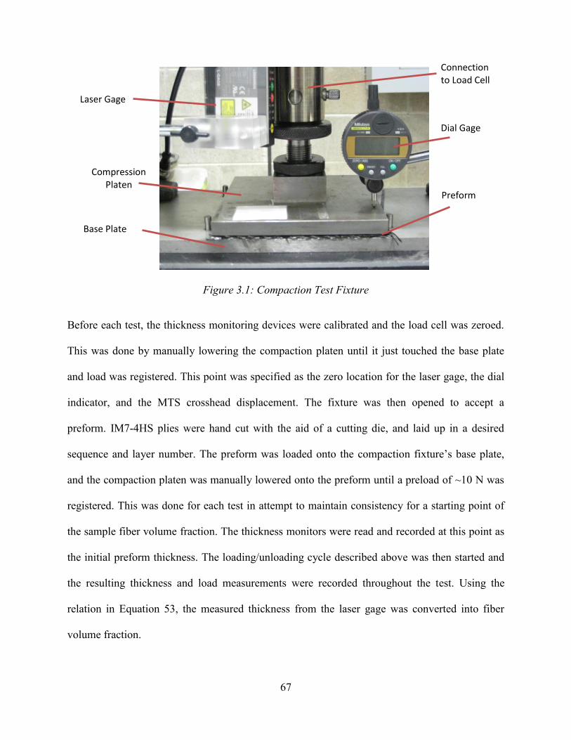
67
Figure 3.1: Compaction Test Fixture
Before each test, the thickness monitoring devices were calibrated and the load cell was zeroed.
This was done by manually lowering the compaction platen until it just touched the base plate
and load was registered. This point was specified as the zero location for the laser gage, the dial
indicator, and the MTS crosshead displacement. The fixture was then opened to accept a
preform. IM7-4HS plies were hand cut with the aid of a cutting die, and laid up in a desired
sequence and layer number. The preform was loaded onto the compaction fixture’s base plate,
and the compaction platen was manually lowered onto the preform until a preload of ~10 N was
registered. This was done for each test in attempt to maintain consistency for a starting point of
the sample fiber volume fraction. The thickness monitors were read and recorded at this point as
the initial preform thickness. The loading/unloading cycle described above was then started and
the resulting thickness and load measurements were recorded throughout the test. Using the
relation in Equation 53, the measured thickness from the laser gage was converted into fiber
volume fraction.
Laser Gage
Compression Platen
Base Plate
Dial Gage
Preform
Connection to Load Cell
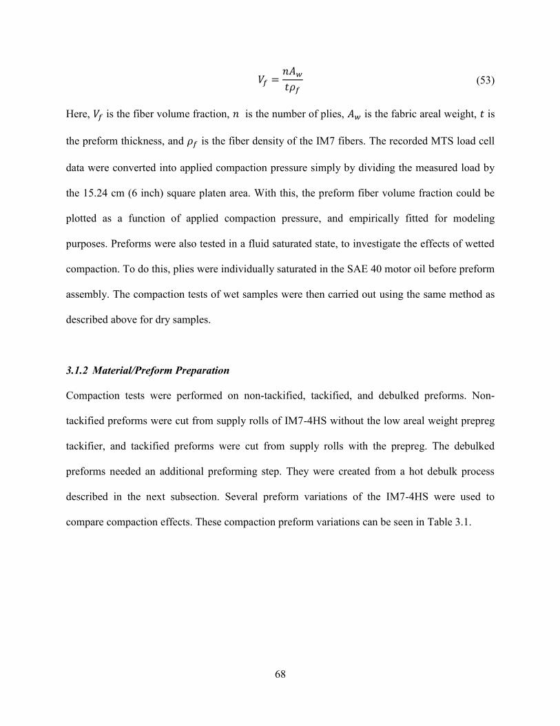
68
𝑉𝑓 =
𝑛𝐴𝑤𝑡𝜌𝑓
(53)
Here, 𝑉𝑓 is the fiber volume fraction, 𝑛 is the number of plies, 𝐴𝑤 is the fabric areal weight, 𝑡 is
the preform thickness, and 𝜌𝑓 is the fiber density of the IM7 fibers. The recorded MTS load cell
data were converted into applied compaction pressure simply by dividing the measured load by
the 15.24 cm (6 inch) square platen area. With this, the preform fiber volume fraction could be
plotted as a function of applied compaction pressure, and empirically fitted for modeling
purposes. Preforms were also tested in a fluid saturated state, to investigate the effects of wetted
compaction. To do this, plies were individually saturated in the SAE 40 motor oil before preform
assembly. The compaction tests of wet samples were then carried out using the same method as
described above for dry samples.
3.1.2 Material/Preform Preparation
Compaction tests were performed on non-tackified, tackified, and debulked preforms. Non-
tackified preforms were cut from supply rolls of IM7-4HS without the low areal weight prepreg
tackifier, and tackified preforms were cut from supply rolls with the prepreg. The debulked
preforms needed an additional preforming step. They were created from a hot debulk process
described in the next subsection. Several preform variations of the IM7-4HS were used to
compare compaction effects. These compaction preform variations can be seen in Table 3.1.
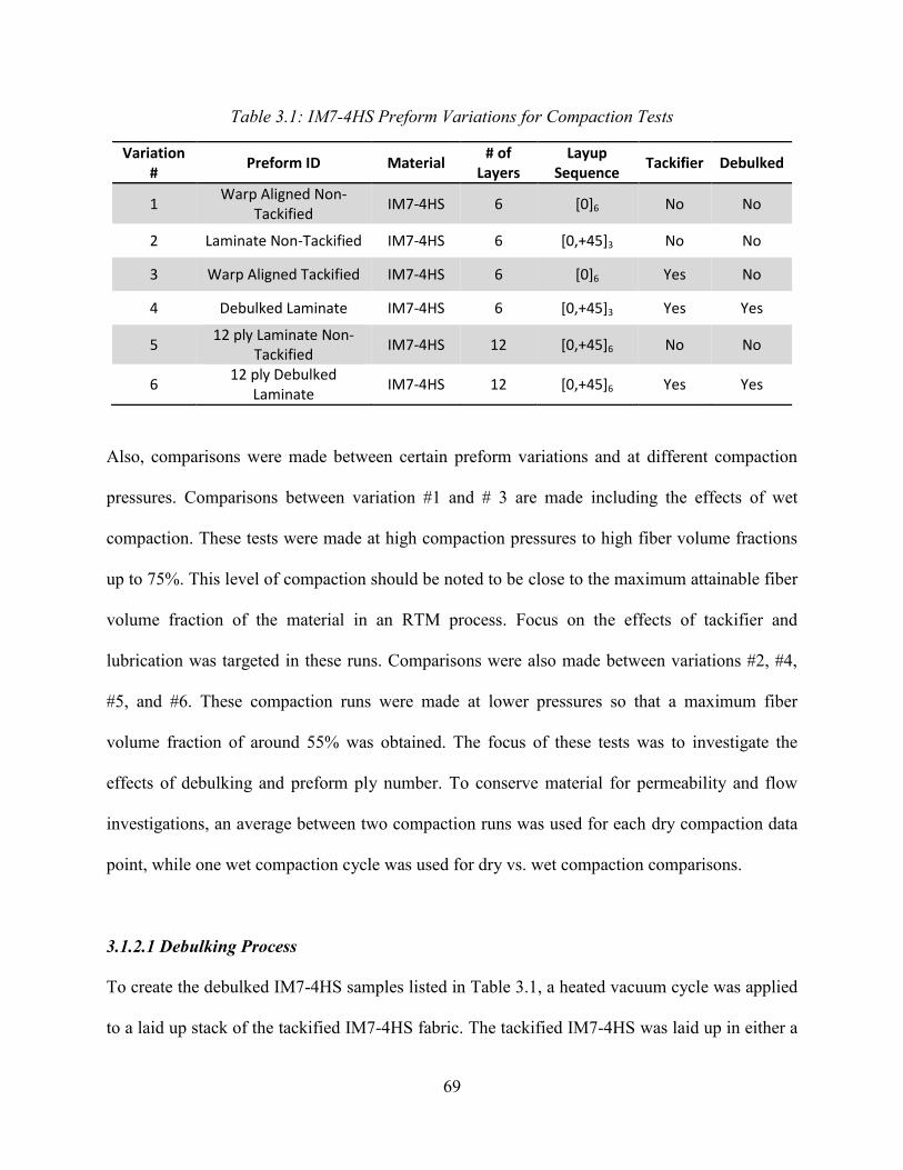
69
Table 3.1: IM7-4HS Preform Variations for Compaction Tests
Variation #
Preform ID Material # of
Layers Layup
Sequence Tackifier Debulked
1 Warp Aligned Non-
Tackified IM7-4HS 6 [0]6 No No
2 Laminate Non-Tackified IM7-4HS 6 [0,+45]3 No No
3 Warp Aligned Tackified IM7-4HS 6 [0]6 Yes No
4 Debulked Laminate IM7-4HS 6 [0,+45]3 Yes Yes
5 12 ply Laminate Non-
Tackified IM7-4HS 12 [0,+45]6 No No
6 12 ply Debulked
Laminate IM7-4HS 12 [0,+45]6 Yes Yes
Also, comparisons were made between certain preform variations and at different compaction
pressures. Comparisons between variation #1 and # 3 are made including the effects of wet
compaction. These tests were made at high compaction pressures to high fiber volume fractions
up to 75%. This level of compaction should be noted to be close to the maximum attainable fiber
volume fraction of the material in an RTM process. Focus on the effects of tackifier and
lubrication was targeted in these runs. Comparisons were also made between variations #2, #4,
#5, and #6. These compaction runs were made at lower pressures so that a maximum fiber
volume fraction of around 55% was obtained. The focus of these tests was to investigate the
effects of debulking and preform ply number. To conserve material for permeability and flow
investigations, an average between two compaction runs was used for each dry compaction data
point, while one wet compaction cycle was used for dry vs. wet compaction comparisons.
3.1.2.1 Debulking Process
To create the debulked IM7-4HS samples listed in Table 3.1, a heated vacuum cycle was applied
to a laid up stack of the tackified IM7-4HS fabric. The tackified IM7-4HS was laid up in either a
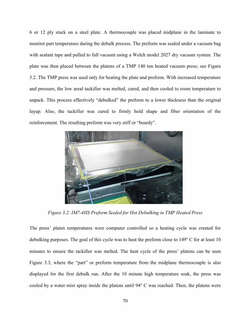
70
6 or 12 ply stack on a steel plate. A thermocouple was placed midplane in the laminate to
monitor part temperature during the debulk process. The preform was sealed under a vacuum bag
with sealant tape and pulled to full vacuum using a Welch model 2027 dry vacuum system. The
plate was then placed between the platens of a TMP 140 ton heated vacuum press; see Figure
3.2. The TMP press was used only for heating the plate and preform. With increased temperature
and pressure, the low areal tackifier was melted, cured, and then cooled to room temperature to
unpack. This process effectively “debulked” the preform to a lower thickness than the original
layup. Also, the tackifier was cured to firmly hold shape and fiber orientation of the
reinforcement. The resulting preform was very stiff or “boardy”.
Figure 3.2: IM7-4HS Preform Sealed for Hot Debulking in TMP Heated Press
The press’ platen temperatures were computer controlled so a heating cycle was created for
debulking purposes. The goal of this cycle was to heat the preform close to 149° C for at least 10
minutes to ensure the tackifier was melted. The heat cycle of the press’ platens can be seen
Figure 3.3, where the “part” or preform temperature from the midplane thermocouple is also
displayed for the first debulk run. After the 10 minute high temperature soak, the press was
cooled by a water mist spray inside the platens until 94° C was reached. Then, the platens were

71
cooled further by flooding their interiors with cold water until they reached 38° C. Vacuum was
then halted and the preform was debagged and allowed to reach room temperature before test
samples were cut.
Figure 3.3: TMP Platen Temperature Cycle for Debulking Process
The debulk cycle took roughly 70 minutes to complete and produced stiff preforms that were
compacted to roughly 45% to 50% fiber volume fraction with the aid of full vacuum pressure.
The interlayer tackifier cured to securely bind together laminate plies. Tackifier melting and
rearrangement was expected in the process, including the likelihood of tows absorbing some of
the melted tackifier. This debulking process was used for several sets of preforms both for
compaction and permeability measurements.
3.2 Results and Discussion
A sample compaction graph is displayed in Figure 3.4. This figure illustrates the general
characteristics of the loading and unloading curves. This specific graph was generated from the
measurements of a 12 ply, non-tackified IM7-4HS laminate sample. The sample, initially at
0
20
40
60
80
100
120
140
160
0 10 20 30 40 50 60 70 80
Tem
pe
ratu
re (
°C)
Time (min)
Part
Platen

72
about 30% fiber volume fraction, was loaded to 105 kPa of compaction pressure then unloaded
until no compaction was present. A maximum fiber volume fraction just under 55% was reached
with these compaction pressures. Note the hysteresis of fiber volume fraction starting and ending
points. After unloading the sample was roughly 8% higher in fiber volume fraction then initially
before the compaction cycle. Although, some of this could be recovered from relaxation over
time, this was not studied here, as typically, only the loading curve is needed to characterize
preforms for RTM applications. Also, consecutive compaction cycles were not run on the IM7-
4HS samples.
Figure 3.4: Typical Preform Compaction Graph (12 Ply Non-tackified IM7-4HS Laminate)
0
0.1
0.2
0.3
0.4
0.5
0.6
0 20 40 60 80 100 120
Fib
er
Vo
lum
e F
ract
ion
, Vf
Comapction Pressure (kPa)
Non-tackified Laminate (12 ply) Loading
Unloading
Unloading
Loading
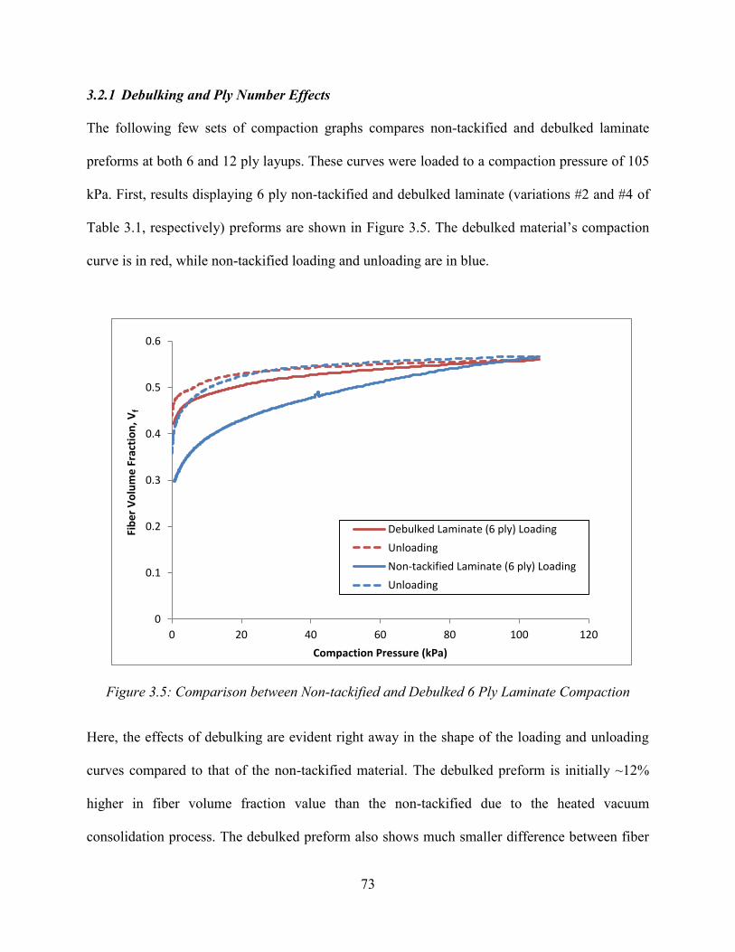
73
3.2.1 Debulking and Ply Number Effects
The following few sets of compaction graphs compares non-tackified and debulked laminate
preforms at both 6 and 12 ply layups. These curves were loaded to a compaction pressure of 105
kPa. First, results displaying 6 ply non-tackified and debulked laminate (variations #2 and #4 of
Table 3.1, respectively) preforms are shown in Figure 3.5. The debulked material’s compaction
curve is in red, while non-tackified loading and unloading are in blue.
Figure 3.5: Comparison between Non-tackified and Debulked 6 Ply Laminate Compaction
Here, the effects of debulking are evident right away in the shape of the loading and unloading
curves compared to that of the non-tackified material. The debulked preform is initially ~12%
higher in fiber volume fraction value than the non-tackified due to the heated vacuum
consolidation process. The debulked preform also shows much smaller difference between fiber
0
0.1
0.2
0.3
0.4
0.5
0.6
0 20 40 60 80 100 120
Fib
er
Vo
lum
e F
ract
ion
, Vf
Compaction Pressure (kPa)
Debulked Laminate (6 ply) Loading
Unloading
Non-tackified Laminate (6 ply) Loading
Unloading
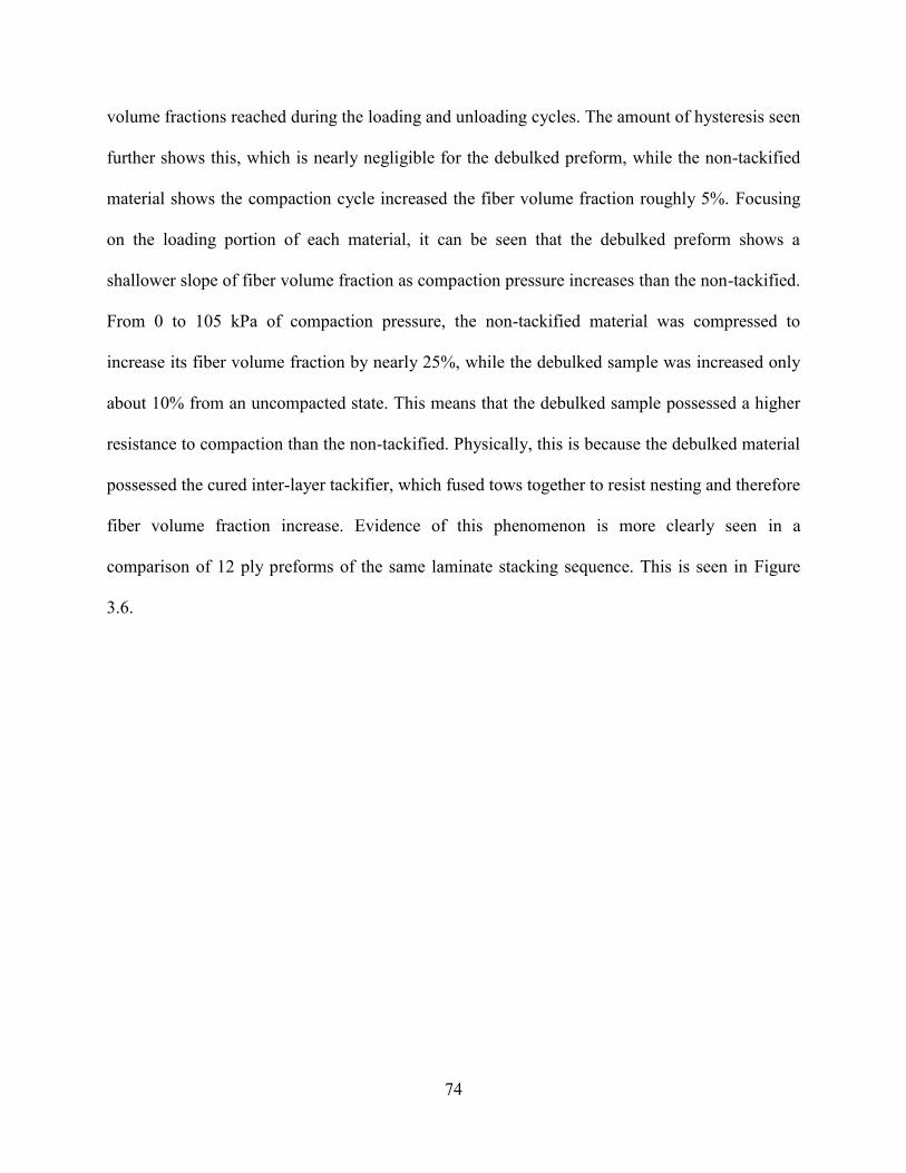
74
volume fractions reached during the loading and unloading cycles. The amount of hysteresis seen
further shows this, which is nearly negligible for the debulked preform, while the non-tackified
material shows the compaction cycle increased the fiber volume fraction roughly 5%. Focusing
on the loading portion of each material, it can be seen that the debulked preform shows a
shallower slope of fiber volume fraction as compaction pressure increases than the non-tackified.
From 0 to 105 kPa of compaction pressure, the non-tackified material was compressed to
increase its fiber volume fraction by nearly 25%, while the debulked sample was increased only
about 10% from an uncompacted state. This means that the debulked sample possessed a higher
resistance to compaction than the non-tackified. Physically, this is because the debulked material
possessed the cured inter-layer tackifier, which fused tows together to resist nesting and therefore
fiber volume fraction increase. Evidence of this phenomenon is more clearly seen in a
comparison of 12 ply preforms of the same laminate stacking sequence. This is seen in Figure
3.6.
75
Figure 3.6: Comparison between Non-tackified and Debulked 12 Ply Laminate Compaction
The 12 ply debulked material showed large resistance compaction pressures. Virtually no
increase in fiber volume fraction was seen on the loading curve. The debulked sample was also
nearly 20% higher in initial fiber volume fraction than the non-tackified material. From these
results it can be concluded that reaching higher fiber volume fraction in debulked samples should
require very high compaction pressures compared to non-debulked.
Now, an overlay of non-tackified laminate IM7-4HS preform layups is shown in Figure 3.7,
where a direct comparison of ply number, 6 versus 12 ply preforms is made. Here, the green
curves relates to the 6 ply preform, while black curves represent the 12 ply preform.
0
0.1
0.2
0.3
0.4
0.5
0.6
0 20 40 60 80 100 120
Fib
er
Vo
lum
e F
ract
ion
, Vf
Compaction Pressure (kPa)
Non-tackified Laminate (12 ply) Loading
Unloading
Debulked Laminate (12 ply) Loading
Unloading
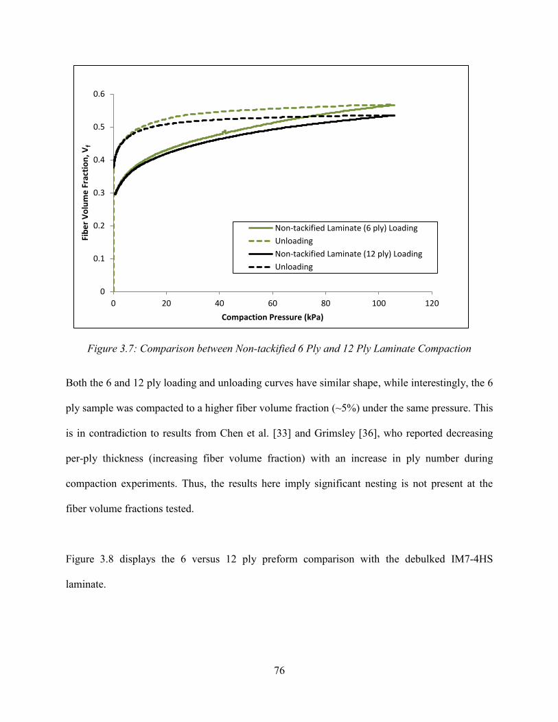
76
Figure 3.7: Comparison between Non-tackified 6 Ply and 12 Ply Laminate Compaction
Both the 6 and 12 ply loading and unloading curves have similar shape, while interestingly, the 6
ply sample was compacted to a higher fiber volume fraction (~5%) under the same pressure. This
is in contradiction to results from Chen et al. [33] and Grimsley [36], who reported decreasing
per-ply thickness (increasing fiber volume fraction) with an increase in ply number during
compaction experiments. Thus, the results here imply significant nesting is not present at the
fiber volume fractions tested.
Figure 3.8 displays the 6 versus 12 ply preform comparison with the debulked IM7-4HS
laminate.
0
0.1
0.2
0.3
0.4
0.5
0.6
0 20 40 60 80 100 120
Fib
er
Vo
lum
e F
ract
ion
, Vf
Compaction Pressure (kPa)
Non-tackified Laminate (6 ply) Loading
Unloading
Non-tackified Laminate (12 ply) Loading
Unloading
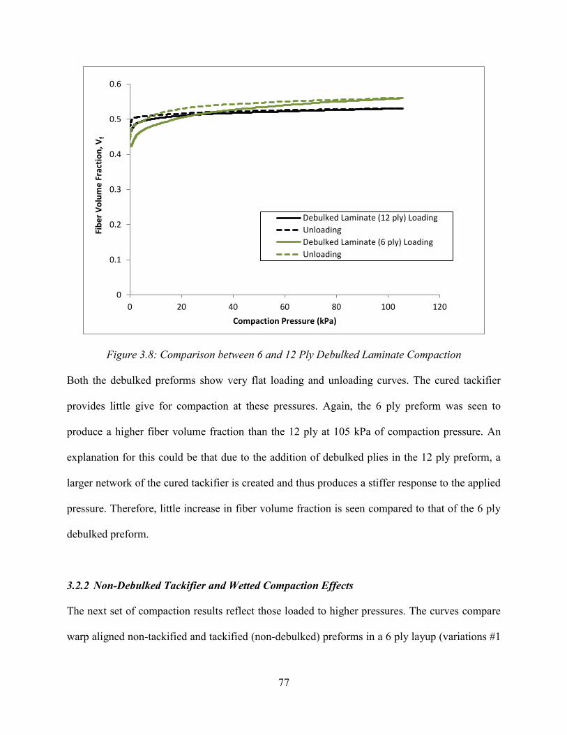
77
Figure 3.8: Comparison between 6 and 12 Ply Debulked Laminate Compaction
Both the debulked preforms show very flat loading and unloading curves. The cured tackifier
provides little give for compaction at these pressures. Again, the 6 ply preform was seen to
produce a higher fiber volume fraction than the 12 ply at 105 kPa of compaction pressure. An
explanation for this could be that due to the addition of debulked plies in the 12 ply preform, a
larger network of the cured tackifier is created and thus produces a stiffer response to the applied
pressure. Therefore, little increase in fiber volume fraction is seen compared to that of the 6 ply
debulked preform.
3.2.2 Non-Debulked Tackifier and Wetted Compaction Effects
The next set of compaction results reflect those loaded to higher pressures. The curves compare
warp aligned non-tackified and tackified (non-debulked) preforms in a 6 ply layup (variations #1
0
0.1
0.2
0.3
0.4
0.5
0.6
0 20 40 60 80 100 120
Fib
er
Vo
lum
e F
ract
ion
, Vf
Compaction Pressure (kPa)
Debulked Laminate (12 ply) Loading
Unloading
Debulked Laminate (6 ply) Loading
Unloading

78
and #3 of Table 3.1, respectively) loaded to 500 kPa. These results also will investigate wet
compaction and the lubricative effect. Figure 3.9 displays a comparison between warp aligned
non-tackified and tackified preforms. Here, the blue color curves represent preforms constructed
of the non-tackified IM7-4HS, whereas the red curves signify the preforms of tackified material,
but not debulked.
Figure 3.9: Comparisons between Non-tackified and Tackified Warp Aligned 6 Ply IM7-4HS Compaction
Here, both the tackified and non-tackified warp aligned preforms were compacted to a similar
fiber volume fraction at maximum pressure. A smaller difference between the loading and
unloading curve in fiber volume fraction was seen for the tackified material compared to the
non-tackified samples. As compaction pressure increased, the slope of the tackified loading
curve became shallower than the non-tackified material. Surprisingly, the loading curve of the
0
0.1
0.2
0.3
0.4
0.5
0.6
0.7
0.8
0 100 200 300 400 500 600
Fib
er
Vo
lum
e F
ract
ion
, Vf
Compaction Pressure (kPa)
Warp Aligned Non-Tackified (6 ply) LoadingUnloadingWarp Aligned Tackified (6ply) LoadingUnloading
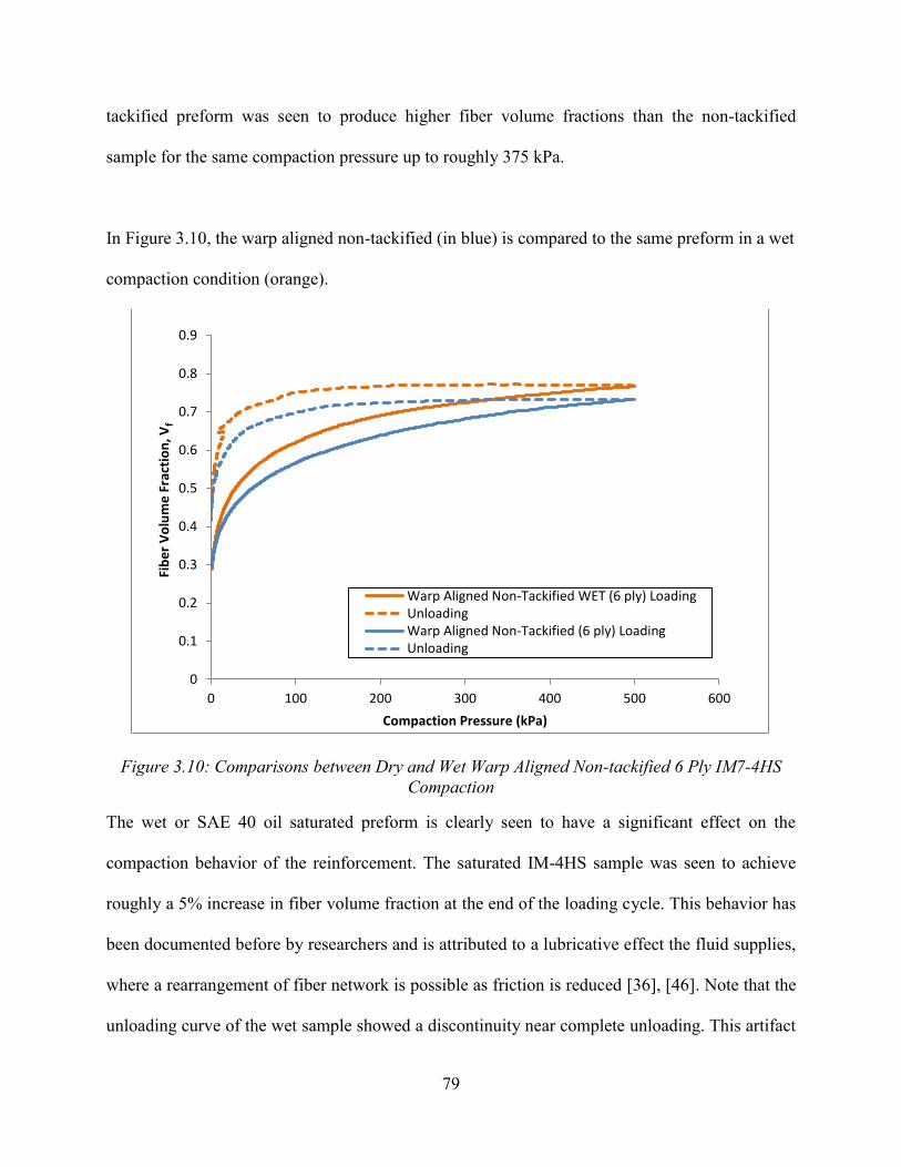
79
tackified preform was seen to produce higher fiber volume fractions than the non-tackified
sample for the same compaction pressure up to roughly 375 kPa.
In Figure 3.10, the warp aligned non-tackified (in blue) is compared to the same preform in a wet
compaction condition (orange).
Figure 3.10: Comparisons between Dry and Wet Warp Aligned Non-tackified 6 Ply IM7-4HS Compaction
The wet or SAE 40 oil saturated preform is clearly seen to have a significant effect on the
compaction behavior of the reinforcement. The saturated IM-4HS sample was seen to achieve
roughly a 5% increase in fiber volume fraction at the end of the loading cycle. This behavior has
been documented before by researchers and is attributed to a lubricative effect the fluid supplies,
where a rearrangement of fiber network is possible as friction is reduced [36], [46]. Note that the
unloading curve of the wet sample showed a discontinuity near complete unloading. This artifact
0
0.1
0.2
0.3
0.4
0.5
0.6
0.7
0.8
0.9
0 100 200 300 400 500 600
Fib
er
Vo
lum
e F
ract
ion
, Vf
Compaction Pressure (kPa)
Warp Aligned Non-Tackified WET (6 ply) LoadingUnloadingWarp Aligned Non-Tackified (6 ply) LoadingUnloading
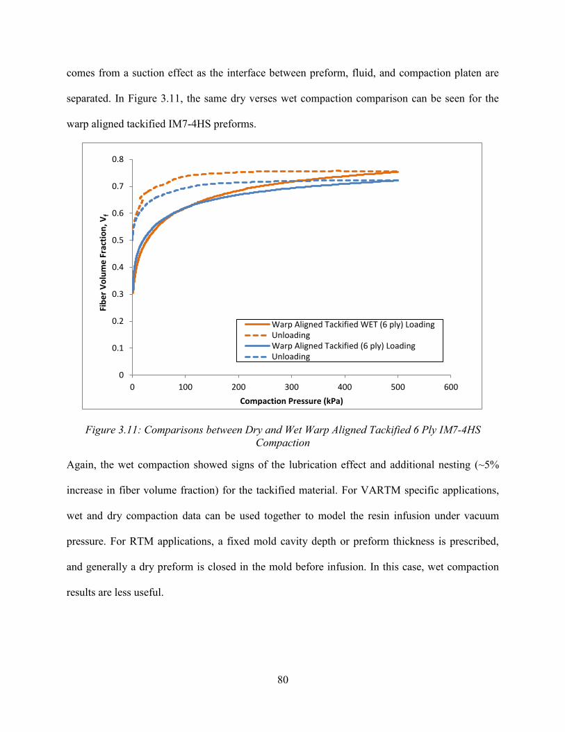
80
comes from a suction effect as the interface between preform, fluid, and compaction platen are
separated. In Figure 3.11, the same dry verses wet compaction comparison can be seen for the
warp aligned tackified IM7-4HS preforms.
Figure 3.11: Comparisons between Dry and Wet Warp Aligned Tackified 6 Ply IM7-4HS Compaction
Again, the wet compaction showed signs of the lubrication effect and additional nesting (~5%
increase in fiber volume fraction) for the tackified material. For VARTM specific applications,
wet and dry compaction data can be used together to model the resin infusion under vacuum
pressure. For RTM applications, a fixed mold cavity depth or preform thickness is prescribed,
and generally a dry preform is closed in the mold before infusion. In this case, wet compaction
results are less useful.
0
0.1
0.2
0.3
0.4
0.5
0.6
0.7
0.8
0 100 200 300 400 500 600
Fib
er
Vo
lum
e F
ract
ion
, Vf
Compaction Pressure (kPa)
Warp Aligned Tackified WET (6 ply) LoadingUnloadingWarp Aligned Tackified (6 ply) LoadingUnloading

81
Finally, wet compaction curves of non-tackified (green) verses tackified (black) IM7-4HS
preforms are presented in Figure 3.12.
Figure 3.12: Comparisons between Non-tackified and Tackified Warp Aligned 6 Ply IM7-4HS Wet Compaction
Very similar compaction behavior is seen between the wet samples of the non-tackified and
tackified IM7-4HS. From this, it may be concluded that the lubrication effect is a dominant
feature of the compressibility of the IM7-4HS, and in this case, makes the presence of tackifier
negligible.
3.3 Conclusions
In this chapter, simple compressibility experiments were described and results were presented on
various IM7-4HS preforms, which correlated applied compaction pressure to fiber volume
fraction. The heated vacuum debulk cycle was also presented, which was used to consolidate
tackified IM7-4HS preforms. Debulking produced very stiff and boardy preforms. The debulking
0
0.1
0.2
0.3
0.4
0.5
0.6
0.7
0.8
0.9
0 100 200 300 400 500 600
Fib
er
Vo
lum
e F
ract
ion
, Vf
Compaction Pressure (kPa)
Warp Aligned Non-Tackified WET (6 ply) LoadingUnloadingWarp Aligned Tackified WET (6 ply) LoadingUnloading

82
process provided pre-compaction to the preforms, where samples were seen to reach between
45% and 50% fiber volume fraction after the cycle was completed. Debulked samples then
showed a large resistance to compaction pressures compared to non-debulked preforms. This
was attributed the cured tackifier fusing tows together, which resisted fiber rearrangement. 12
ply debulked experiments were seen to resist compaction greater than those of 6 ply. Tackified,
but non-debulked samples also displayed some resistance to compaction at high pressures,
although not as great as the debulked material. This is because the unprocessed inter-layer
tackifier was not cured to fuse tows, so some nesting was still achievable. Further wetted
compaction experiments (SAE 40 oil saturated preforms) showed results consistent with
literature, where higher fiber content was achievable under the same compaction pressures than
dry compaction due to the lubrication effect. Also, the wetted compaction curve comparison
between tackified and non-tackified preforms showed nearly identical fiber volume fractions for
the same applied compaction pressures. Notably, the wetting effect was deemed to make the
presence of tackifier (non-debulked) negligible. Further work could quantify the amount of
spring-back obtained among non-tackified, tackified, and debulked IM7-4HS preforms.
Regarding application to LCM, Shih and Lee [10] stated that an ideal tackifier should be able to
prevent spring-back to maintain good preform dimension control. While spring-back and
relaxation were not explicitly studied in this investigation, it is clear that upon debulking of
tackified IM7-4HS, a very stiff and compaction resistant preform is created. For RTM then,
debulking may be beneficial in terms of dimensional control. Although if preform fiber volume
fractions are desired that are higher than what vacuum compaction can achieve, debulking in
rigid molds may be necessary. Compaction experiments at high compaction pressures (like the

83
ones done in this study) then would become helpful. Care should be taken regarding debulking,
to ensure the preform is not compacted to a smaller thickness than what will be obtained in an
RTM mold. If this is the case, race-tracking around the preform may occur [10]. Permeability
and flow through IM7-4HS preforms including debulked samples will be explored next in
Chapter 4.
84
4. Saturated Permeability
Saturated permeability characterization methods have been used for years to provide input
parameters for Darcian flow based process models in LCM. While in some cases, these methods
have been noted to produce different flow and permeability than those of unsaturated flow (flow
native to the LCM process) [139], their data output per sample is much higher. Saturated
measurements allow characterization of permeability across multiple fiber volume fractions with
one sample, while unsaturated methods can only produce one data point per sample. Saturated
permeability measurements then provide a good baseline method for characterization of the IM7-
4HS preforms. This chapter will present the saturated permeability measurement techniques and
fixture setup for both in-plane and transverse characterization. The effects of the inter-layer
tackifier, sample debulking, layup, and ply number on preform permeability are also presented.
Important inferences regarding tackifier effects will be noted in reference to composite
manufacturing. The baseline results produced here will be used to compare with unsaturated
methods in Chapter 5.
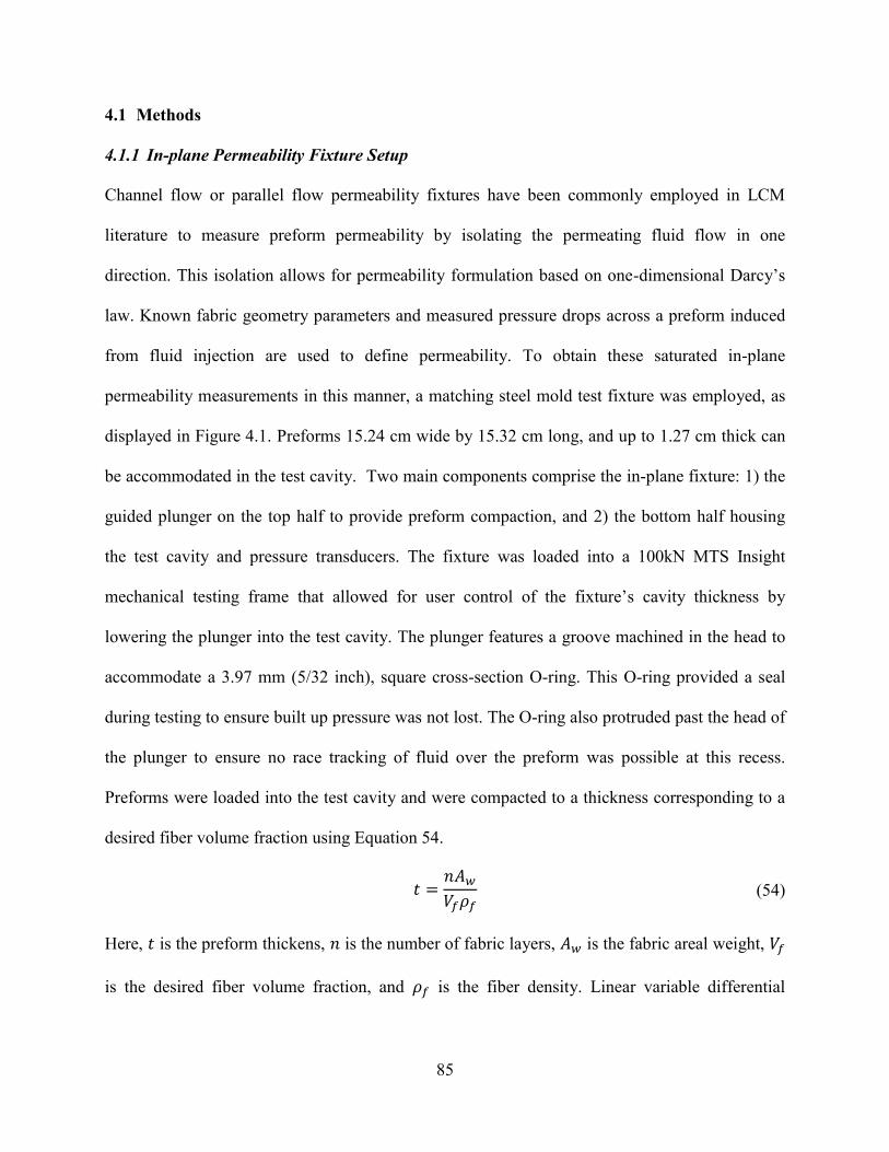
85
4.1 Methods
4.1.1 In-plane Permeability Fixture Setup
Channel flow or parallel flow permeability fixtures have been commonly employed in LCM
literature to measure preform permeability by isolating the permeating fluid flow in one
direction. This isolation allows for permeability formulation based on one-dimensional Darcy’s
law. Known fabric geometry parameters and measured pressure drops across a preform induced
from fluid injection are used to define permeability. To obtain these saturated in-plane
permeability measurements in this manner, a matching steel mold test fixture was employed, as
displayed in Figure 4.1. Preforms 15.24 cm wide by 15.32 cm long, and up to 1.27 cm thick can
be accommodated in the test cavity. Two main components comprise the in-plane fixture: 1) the
guided plunger on the top half to provide preform compaction, and 2) the bottom half housing
the test cavity and pressure transducers. The fixture was loaded into a 100kN MTS Insight
mechanical testing frame that allowed for user control of the fixture’s cavity thickness by
lowering the plunger into the test cavity. The plunger features a groove machined in the head to
accommodate a 3.97 mm (5/32 inch), square cross-section O-ring. This O-ring provided a seal
during testing to ensure built up pressure was not lost. The O-ring also protruded past the head of
the plunger to ensure no race tracking of fluid over the preform was possible at this recess.
Preforms were loaded into the test cavity and were compacted to a thickness corresponding to a
desired fiber volume fraction using Equation 54.
𝑡 =
𝑛𝐴𝑤𝑉𝑓𝜌𝑓
(54)
Here, 𝑡 is the preform thickens, 𝑛 is the number of fabric layers, 𝐴𝑤 is the fabric areal weight, 𝑉𝑓
is the desired fiber volume fraction, and 𝜌𝑓 is the fiber density. Linear variable differential
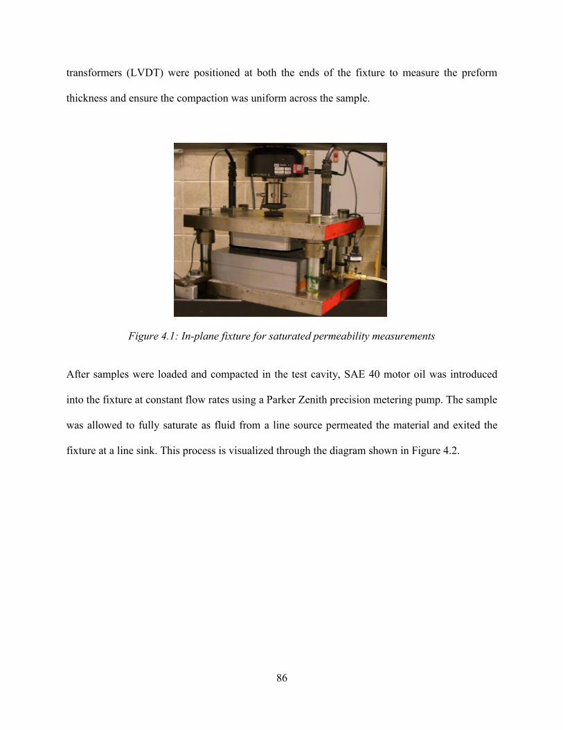
86
transformers (LVDT) were positioned at both the ends of the fixture to measure the preform
thickness and ensure the compaction was uniform across the sample.
Figure 4.1: In-plane fixture for saturated permeability measurements
After samples were loaded and compacted in the test cavity, SAE 40 motor oil was introduced
into the fixture at constant flow rates using a Parker Zenith precision metering pump. The sample
was allowed to fully saturate as fluid from a line source permeated the material and exited the
fixture at a line sink. This process is visualized through the diagram shown in Figure 4.2.
87
Figure 4.2: In-plane Fixture Test Diagram. Top and Front View.
Steady-state was reached when inlet pressure readouts from the in-line pressure transducer
(Omega PX180-100GV) and the outlet digital pressure gage (Omega DPG1000B-15G) remained
constant after full preform saturation. Pressure drops across the preform were measured for the
set fiber volume fraction at multiple flow rates. These pressure drops are plotted versus the flow
rates to attain a slope, m, which can be used in an altered form of Darcy’s law (Equation 55) to
calculate the average permeability of the preform. Permeability is defined by 𝑆 while µ is the
fluid viscosity, 𝐿 is the preform length in the direction of the flow, and 𝐴 is the area normal to
the flow.
𝑆 = µ𝑚
𝐿
𝐴 (55)
Compaction Force
LVDT
Preform
Front View
Inlet
Pressure
Transducer
Top View
Fluid Inlet
Fluid
Outlet
Line Source Line Sink
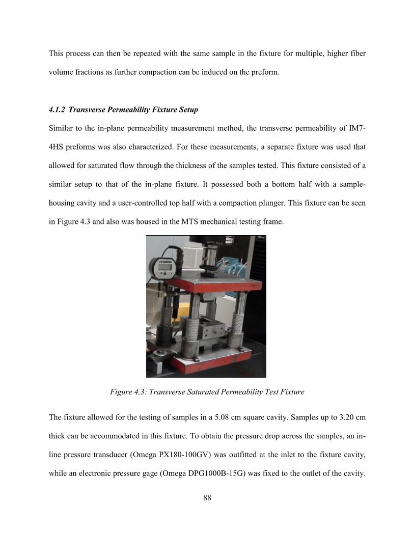
88
This process can then be repeated with the same sample in the fixture for multiple, higher fiber
volume fractions as further compaction can be induced on the preform.
4.1.2 Transverse Permeability Fixture Setup
Similar to the in-plane permeability measurement method, the transverse permeability of IM7-
4HS preforms was also characterized. For these measurements, a separate fixture was used that
allowed for saturated flow through the thickness of the samples tested. This fixture consisted of a
similar setup to that of the in-plane fixture. It possessed both a bottom half with a sample-
housing cavity and a user-controlled top half with a compaction plunger. This fixture can be seen
in Figure 4.3 and also was housed in the MTS mechanical testing frame.
Figure 4.3: Transverse Saturated Permeability Test Fixture
The fixture allowed for the testing of samples in a 5.08 cm square cavity. Samples up to 3.20 cm
thick can be accommodated in this fixture. To obtain the pressure drop across the samples, an in-
line pressure transducer (Omega PX180-100GV) was outfitted at the inlet to the fixture cavity,
while an electronic pressure gage (Omega DPG1000B-15G) was fixed to the outlet of the cavity.
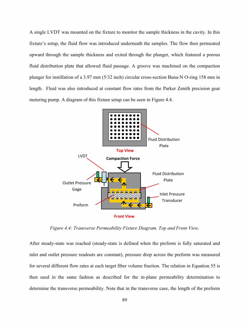
89
A single LVDT was mounted on the fixture to monitor the sample thickness in the cavity. In this
fixture’s setup, the fluid flow was introduced underneath the samples. The flow then permeated
upward through the sample thickness and exited through the plunger, which featured a porous
fluid distribution plate that allowed fluid passage. A groove was machined on the compaction
plunger for instillation of a 3.97 mm (5/32 inch) circular cross-section Buna-N O-ring 158 mm in
length. Fluid was also introduced at constant flow rates from the Parker Zenith precision gear
metering pump. A diagram of this fixture setup can be seen in Figure 4.4.
Figure 4.4: Transverse Permeability Fixture Diagram. Top and Front View.
After steady-state was reached (steady-state is defined when the preform is fully saturated and
inlet and outlet pressure readouts are constant), pressure drop across the preform was measured
for several different flow rates at each target fiber volume fraction. The relation in Equation 55 is
then used in the same fashion as described for the in-plane permeability determination to
determine the transverse permeability. Note that in the transverse case, the length of the preform
Compaction Force LVDT
Preform
Front View
Top View
Outlet Pressure
Gage
Fluid Distribution
Plate
Fluid Distribution
Plate
Inlet Pressure
Transducer

90
in the direction of flow is the sample thickness. Gravitational effects in this transverse setup were
not included in the permeability measurements as they are small compared to the pressure drop
produced at the supplied flow rates.
4.1.3 Material/Preform Preparation
Several different preforms of IM7-4HS fabric were constructed for the saturated permeability
comparison. These preform variations were used to determine the effects of tackifier, debulking,
layup sequence, and ply number on saturated permeability. The in-plane and transverse samples
created are summarized in Table 4.1. Preforms were produced by hand cutting individual plies
from either tackified or non-tackified rolls of the IM7-4HS with a fabric cutting wheel. Exact
cutting templates of the fixture cavity dimensions were machined from aluminum blocks to
ensure ply-by-ply consistency and precise in-cavity fit.
Table 4.1: IM7-4HS Preform Variations for Saturated Permeability Tests
Variation #
Preform ID Material # of
Layers Layup
Sequence Tackifier Debulked
1 Warp Aligned Non-
Tackified IM7-4HS 6 [0]6 No No
2 Laminate Non-Tackified IM7-4HS 6 [0,+45]3 No No
3 Warp Aligned Tackified IM7-4HS 6 [0]6 Yes No
4 Debulked Laminate IM7-4HS 6 [0,+45]3 Yes Yes
5 12 ply Laminate Non-
Tackified IM7-4HS 12 [0,+45]6 No No
6 12 ply Debulked
Laminate IM7-4HS 12 [0,+45]6 Yes Yes
Rolls of the tackified IM7-4HS fabric were stored in a freezer to prevent cure of the pre-
impregnated resin. To prepare tackified preforms, the rolls of material were taken out of the
freezer, allowed to reach room temperature, cut, and then laid up. The debulked preforms were

91
produced by laying up the cut sheets of tackified IM7-4HS fabric and then exposing the preform
to the hot debulk cycle described in Chapter 3. They were also allowed to reach ambient
temperature before saturated testing took place.
4.1.4 Permeability Measurement Procedure
Before any in-plane or transverse saturated permeability measurements took place, the Parker
Zenith constant flow rate pump was calibrated. To do this, the SAE 40 motor oil was pumped
through the equipment at flow rates ranging from 1 cc/min to 20 cc/min into a container placed
on Mettler Toledo SB1600 scale. At each flow rate, the oil was pumped into the container for 1
minute, and the weight of the fluid was recorded. Knowing the density of the oil, the weight
collected and the elapsed time, an average actual flow rate could be calculated and compared to
the pump’s setting.
Both the in-plane and transverse fixtures were installed on the baseplate of a 100 kN MTS
Insight material testing machine. The plunger of the fixture was connected to the load cell
mounted in the crosshead. The crosshead displacement and load cell measurements were
recorded the MTS TestWorks controlled system. On a separate lab computer, LabVIEW
programs were written specifically for both the in-plane and transverse setup. These LabVIEW
programs were used in conjunction with a NI 9219 data acquisition system, which was hard
wired to both the LVDTs and the pressure transducers. With this, the instantaneous LVDT
readouts were displayed and recorded, and the pressures were be recorded over time and
averaged for pressure drop measurements in permeability.
92
4.1.4.1 In-plane Procedure: Step-by-Step
In-plane IM7-4HS preforms were each tested in 3 different flow direction: along the warp (0°),
along the weft/fill (90° and perpendicular to the warp), and at 45° from the warp. This was done
by cutting the preforms at different angles so that the apparent flow path was in these directions.
The measured permeabilities in the 0°, 90°, and 45° are referred to as 𝑆𝑥𝑥, 𝑆𝑦𝑦, and 𝑆𝑥𝑥′,
respectively. Measuring the in-plane permeability of each of these directions allowed the
principal permeabilities (𝑆11 and 𝑆22) to be determined from a tensor transformation, as well as
the orientation of the first principal permeability (𝛽). This was done with a simple MATLAB
script, which can be found in Appendix C. The sensitivity of the angle 𝛽, as a product of 3
saturated channel flow tests, will be further discussed in the results and discussion portion of this
chapter.
To measure each preform of the IM7-4HS material, first the fabric was cut from rolls of IM7-
4HS that were either with or without the prepreg tackifier. The samples were laid up according to
the stacking sequences given in Table 4.1. Next, the LVDTs on the in-plane fixture were
recalibrated. This was done by manually lowering the compaction plunger into the empty cavity
of the fixture until significant load was measured on the load cell, meaning that the plunger had
made contact with the bottom of the test cavity. This was designated as zero thickness for the
LVDTs, as well as, for the MTS crosshead displacement readout. The fixture was then opened to
accept the IM7-4HS sample at the appropriate flow angle. A square O-ring, with the dimensions
specified earlier was cut from a bulk supply, glued, and placed in the groove machined on the
plunger head. The O-ring was then lubricated with Dow Corning’s Molykote 111 and the
plunger was slowly lowered into the test cavity as the O-ring created a seal. The plunger was

93
allowed to compact the fiber sample in the cavity until a specific thickness was reached that
corresponded with the desired levels of fiber volume fraction. The areal weight relation in
Equation 2 was used to do this. The frictional forces from the fixture guide posts entering the
couplings were too significant to allow the compaction of the IM7-4HS samples to be defined
from compaction pressure measured by the MTS load cell. Once the first level of compaction
was reached, the test fluid (SAE 40 motor oil) was supplied from the Parker Zenith metering
pump at low flow rates generally in the range of 1 cc/min to 10 cc/min. Low flow rates were
used so that fluid pressures generated did not exceed the inlet pressure transducer limit of 690
kPa. In Chapter 6, higher flow rates were used and different measurement equipment was
employed, which will be described in detail there. Once full saturation and steady-state were
reached for a test sample, the pressure drop across the preform was measured at multiple flow
rates (generally 4 to 5 flow rates per fiber volume fraction level). The pump was stopped, further
compaction on the sample was applied to achieve a higher desired fiber volume fraction level,
and the measurement process was repeated. For each IM7-4HS preform, fiber volume fractions
of 50%, 55% and 60% were targeted. This range represents a practical area of interest for RTM
manufacturing. If at any point, signs of pressure leakage or if test fluid was seen leaking out from
the O-ring seal, the test was halted and data was not used.
4.1.4.2 Transverse Procedure: Step-by-Step
The procedure used for transverse permeability measurements is very similar to the in-plane
setup. The transverse fixture included a single LVDT that was recalibrated before each run using
the same technique described in the in-plane step-by-step process. Smaller 5.08 x 5.08 cm
samples were cut based on the stacking sequence of Table 4.1. Circular O-rings were cut and

94
lubricated to seal flow on the plunger’s head. Also, the same sample target fiber volume fractions
were used for through-thickness permeability. Flow rates in the range of 1 cc/min to 10 cc/min
were generally used for transverse permeation.
4.2 Results and Discussion
For each saturated data point, a target minimum of 3 tests was made, although a few variations
were repeated fewer times due to material supply. This means that for each flow direction (𝑆𝑥𝑥,
𝑆𝑦𝑦, 𝑆𝑥𝑥′, or 𝑆𝑧𝑧), and at each fiber volume fraction, multiple tests were made to establish an
average and standard deviation. It should also be noted that each saturated test would take
approximately 3 hours to complete (this includes sample cutting, lay up, and permeability
measurement at the three target fiber volume fractions). This results section will only display
graphical representations of a pertinent selection of the entire measurement set because of the
large amount of data produced. The entire body of raw saturated permeability results can be
found in Appendix A. The results are graphically presented are chosen so that the effects of fiber
volume fraction, tackifier, layup, debulking, and ply number on IM7-4HS permeability can be
examined.
4.2.1 In-plane Permeability Results
A total of 62 samples were cut and laid up amounting to 174 separate saturated in-plane
permeability measurements at the specific fiber volume fractions of interest (50%, 55% and
60%). A typical flow rate versus pressure drop curve for a saturated permeability measurement
can be seen in Figure 4.5. The solid lines are linear regressions of each data set. The slope and R-
squared value of each regression are also displayed on the graph. These data are from a debulked
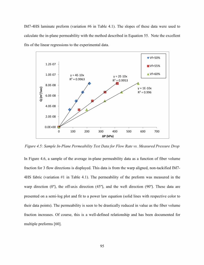
95
IM7-4HS laminate preform (variation #6 in Table 4.1). The slopes of these data were used to
calculate the in-plane permeability with the method described in Equation 55. Note the excellent
fits of the linear regressions to the experimental data.
Figure 4.5: Sample In-Plane Permeability Test Data for Flow Rate vs. Measured Pressure Drop
In Figure 4.6, a sample of the average in-plane permeability data as a function of fiber volume
fraction for 3 flow directions is displayed. This data is from the warp aligned, non-tackified IM7-
4HS fabric (variation #1 in Table 4.1). The permeability of the preform was measured in the
warp direction (0°), the off-axis direction (45°), and the weft direction (90°). These data are
presented on a semi-log plot and fit to a power law equation (solid lines with respective color to
their data points). The permeability is seen to be drastically reduced in value as the fiber volume
fraction increases. Of course, this is a well-defined relationship and has been documented for
multiple preforms [60].
y = 4E-10x R² = 0.9963
y = 2E-10x R² = 0.9953
y = 1E-10x R² = 0.996
0.0E+00
2.0E-08
4.0E-08
6.0E-08
8.0E-08
1.0E-07
1.2E-07
0 100 200 300 400 500 600 700
Q (
m3/s
ec)
ΔP (kPa)
Vf=50%
Vf=55%
Vf=60%
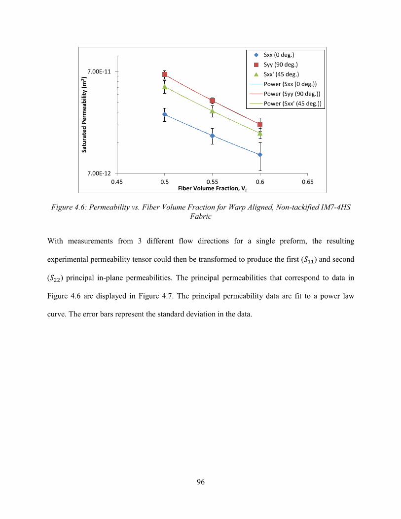
96
Figure 4.6: Permeability vs. Fiber Volume Fraction for Warp Aligned, Non-tackified IM7-4HS Fabric
With measurements from 3 different flow directions for a single preform, the resulting
experimental permeability tensor could then be transformed to produce the first (𝑆11) and second
(𝑆22) principal in-plane permeabilities. The principal permeabilities that correspond to data in
Figure 4.6 are displayed in Figure 4.7. The principal permeability data are fit to a power law
curve. The error bars represent the standard deviation in the data.
7.00E-12
7.00E-11
0.45 0.5 0.55 0.6 0.65
Satu
rate
d P
erm
eab
ility
(m
2 )
Fiber Volume Fraction, Vf
Sxx (0 deg.)
Syy (90 deg.)
Sxx' (45 deg.)
Power (Sxx (0 deg.))
Power (Syy (90 deg.))
Power (Sxx' (45 deg.))

97
Figure 4.7: Principal Permeability vs. Fiber Volume Fraction for Warp Aligned, Non-tackified IM7-4HS Fabric
For this specific warp-aligned preform, the permeability in along the warp axis (0°) of the
material was seen to be much less permeable compared to flow in the weft (90°) direction. The
45° permeability measurements fell between values for the warp and weft. The resulting
principal permeabilities were seen to be slightly higher and slightly lower in value than the weft
and warp directions, respectively. From this, one can assume that orientation of first principal
permeability, or 𝛽 angle is approximately 90° from the warp. Further discussion on the 𝛽 angle
determination and variability will be made later.
4.2.1.1 Fiber Volume Fraction, Layup, Tackifier, and Debulking Effects
After calculating principal permeabilities for all preforms tested, comparisons among layup,
tackifier content, and debulking effects could be made. A comparison of all the 6 ply IM7-4HS
layups can be seen at 55% fiber volume fraction in Figure 4.8. This specific fiber volume
fraction was used to compare preforms types due to the difficulties and anomalies experienced at
6.00E-12
6.00E-11
0.45 0.5 0.55 0.6 0.65
Satu
rate
d P
erm
eab
ility
(m
2 )
Fiber Volume Fraction, Vf
Sxx (0 deg.)
Syy (90 deg.)
Sxx' (45 deg.)
S11
S22
Power (S11)
Power (S22)
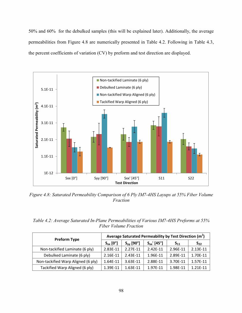
98
50% and 60% for the debulked samples (this will be explained later). Additionally, the average
permeabilities from Figure 4.8 are numerically presented in Table 4.2. Following in Table 4.3,
the percent coefficients of variation (CV) by preform and test direction are displayed.
Figure 4.8: Saturated Permeability Comparison of 6 Ply IM7-4HS Layups at 55% Fiber Volume Fraction
Table 4.2: Average Saturated In-Plane Permeabilities of Various IM7-4HS Preforms at 55% Fiber Volume Fraction
Preform Type Average Saturated Permeability by Test Direction (m2)
Sxx [0°] Syy [90°] Sxx' [45°] S11 S22
Non-tackified Laminate (6 ply) 2.83E-11 2.27E-11 2.42E-11 2.96E-11 2.13E-11
Debulked Laminate (6 ply) 2.16E-11 2.43E-11 1.96E-11 2.89E-11 1.70E-11
Non-tackified Warp Aligned (6 ply) 1.64E-11 3.63E-11 2.88E-11 3.70E-11 1.57E-11
Tackified Warp Aligned (6 ply) 1.39E-11 1.63E-11 1.97E-11 1.98E-11 1.21E-11
1E-12
1.1E-11
2.1E-11
3.1E-11
4.1E-11
5.1E-11
Sxx [0°] Syy [90°] Sxx' [45°] S11 S22
Satu
rate
d P
erm
eab
ility
(m
2)
Test Direction
Non-tackified Laminate (6 ply)
Debulked Laminate (6 ply)
Non-tackified Warp Aligned (6 ply)
Tackified Warp Aligned (6 ply)
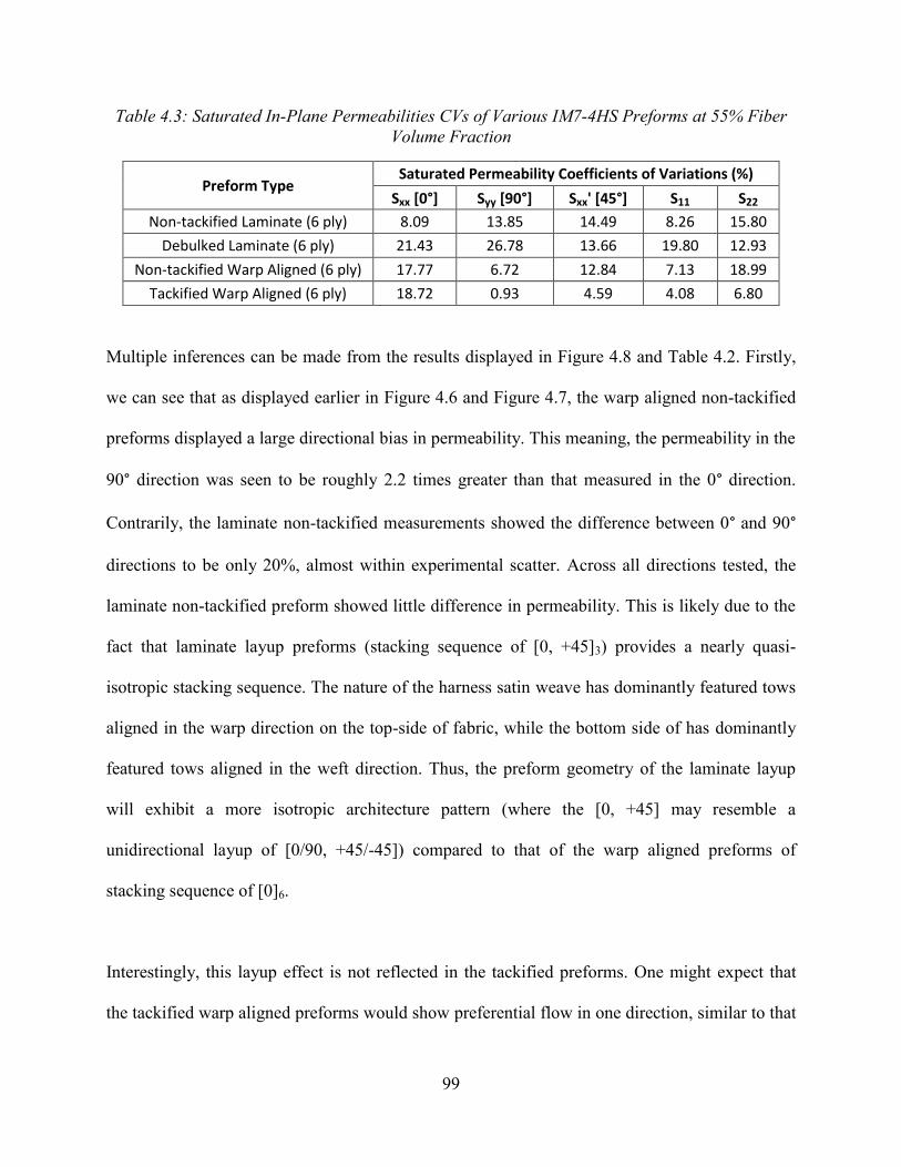
99
Table 4.3: Saturated In-Plane Permeabilities CVs of Various IM7-4HS Preforms at 55% Fiber Volume Fraction
Preform Type Saturated Permeability Coefficients of Variations (%)
Sxx [0°] Syy [90°] Sxx' [45°] S11 S22
Non-tackified Laminate (6 ply) 8.09 13.85 14.49 8.26 15.80
Debulked Laminate (6 ply) 21.43 26.78 13.66 19.80 12.93
Non-tackified Warp Aligned (6 ply) 17.77 6.72 12.84 7.13 18.99
Tackified Warp Aligned (6 ply) 18.72 0.93 4.59 4.08 6.80
Multiple inferences can be made from the results displayed in Figure 4.8 and Table 4.2. Firstly,
we can see that as displayed earlier in Figure 4.6 and Figure 4.7, the warp aligned non-tackified
preforms displayed a large directional bias in permeability. This meaning, the permeability in the
90° direction was seen to be roughly 2.2 times greater than that measured in the 0° direction.
Contrarily, the laminate non-tackified measurements showed the difference between 0° and 90°
directions to be only 20%, almost within experimental scatter. Across all directions tested, the
laminate non-tackified preform showed little difference in permeability. This is likely due to the
fact that laminate layup preforms (stacking sequence of [0, +45]3) provides a nearly quasi-
isotropic stacking sequence. The nature of the harness satin weave has dominantly featured tows
aligned in the warp direction on the top-side of fabric, while the bottom side of has dominantly
featured tows aligned in the weft direction. Thus, the preform geometry of the laminate layup
will exhibit a more isotropic architecture pattern (where the [0, +45] may resemble a
unidirectional layup of [0/90, +45/-45]) compared to that of the warp aligned preforms of
stacking sequence of [0]6.
Interestingly, this layup effect is not reflected in the tackified preforms. One might expect that
the tackified warp aligned preforms would show preferential flow in one direction, similar to that

100
of the non-tackified warp aligned preforms (where permeability is much higher in the 90°
direction than the other directions tested). As seen in Figure 4.8, the warp aligned tackified
preforms showed only a 17% difference between 𝑆𝑥𝑥 and 𝑆𝑦𝑦 permeability, which is within the
experimental scatter of the 𝑆𝑥𝑥 measurements. Thus, the inter-layer tackifier appears to aid in
creating a more isotropic in-plane permeability by greatly reducing the 𝑆𝑦𝑦 value (roughly 2.2
times less) compared to the non-tackified warp aligned preforms. Further, the addition of
tackifier appears to have little effect on permeability measured in the 0° direction. The presence
of tackifier for the warp aligned preforms showed only a 15% drop in permeability, which was
well within the experimental scatter for both preforms. Explanation for this effect may be due to
the manufacturing process, and how the tackifier is applied.
Effects from the debulk cycle on preform permeability can also be gleaned by comparing the
non-tackified laminate preforms to the debulked laminate preforms. It can be seen that, rather
surprisingly, no significant difference in permeability was registered between the two laminates.
This may be best explained by the solidification that occurs as results of the debulking process.
Once the tackifier is heated in the debulk process, it melts and flows through the preform by the
vacuum pressure, and then goes through an irreversible chemical change in curing. This
essentially fuses the tows in place at roughly 50% fiber volume fraction, producing very stiff
preforms. This cured tackifier aids to resist nesting of the fibers and tows upon compression in
the permeability fixture. Nesting, of course, reduces local permeability through the increase in
local fiber volume fraction. A simple schematic diagram of tows of tackified (non-debulked) and
debulked preforms is seen Figure 4.9 to illustrate this point.
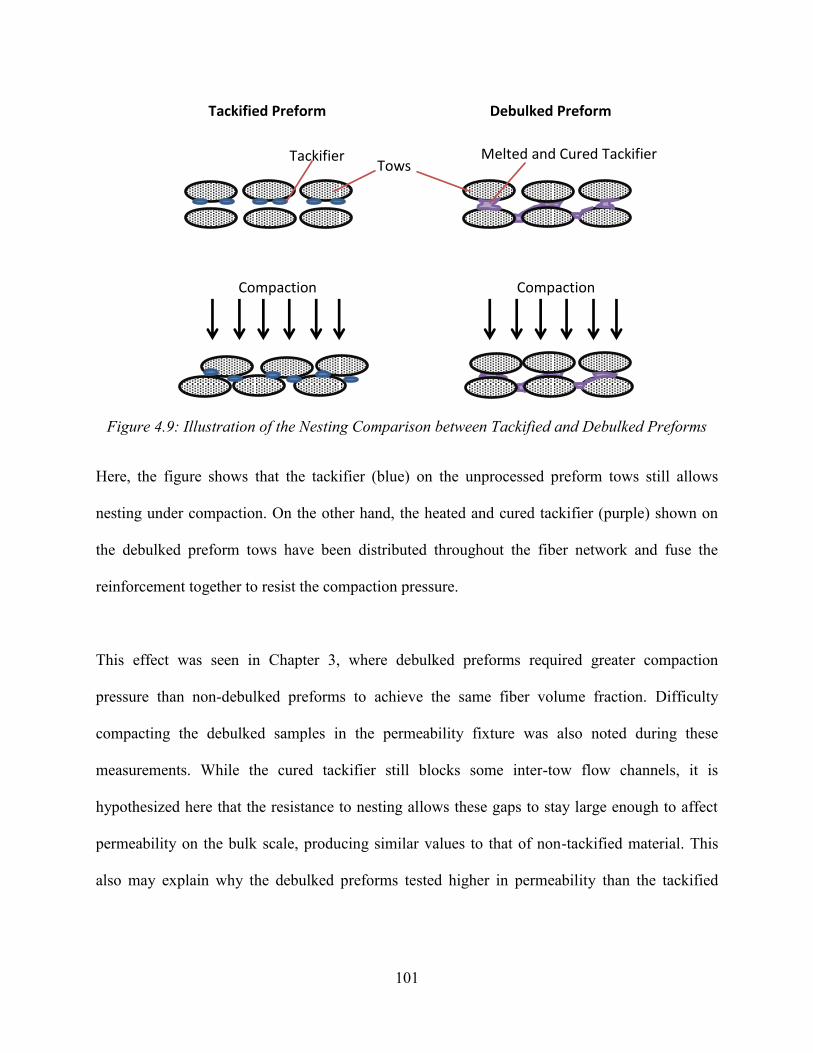
101
Figure 4.9: Illustration of the Nesting Comparison between Tackified and Debulked Preforms
Here, the figure shows that the tackifier (blue) on the unprocessed preform tows still allows
nesting under compaction. On the other hand, the heated and cured tackifier (purple) shown on
the debulked preform tows have been distributed throughout the fiber network and fuse the
reinforcement together to resist the compaction pressure.
This effect was seen in Chapter 3, where debulked preforms required greater compaction
pressure than non-debulked preforms to achieve the same fiber volume fraction. Difficulty
compacting the debulked samples in the permeability fixture was also noted during these
measurements. While the cured tackifier still blocks some inter-tow flow channels, it is
hypothesized here that the resistance to nesting allows these gaps to stay large enough to affect
permeability on the bulk scale, producing similar values to that of non-tackified material. This
also may explain why the debulked preforms tested higher in permeability than the tackified
Debulked Preform Tackified Preform
Compaction Compaction
Tackifier Tows
Melted and Cured Tackifier
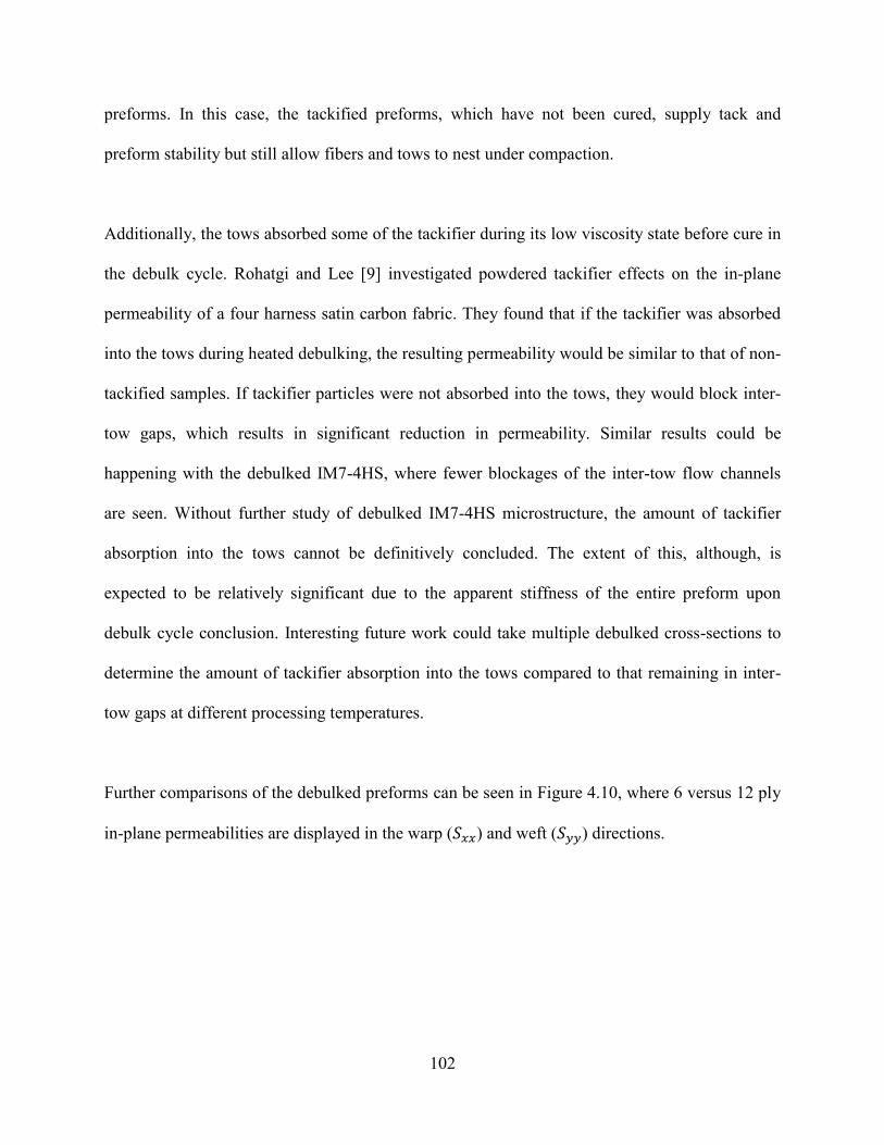
102
preforms. In this case, the tackified preforms, which have not been cured, supply tack and
preform stability but still allow fibers and tows to nest under compaction.
Additionally, the tows absorbed some of the tackifier during its low viscosity state before cure in
the debulk cycle. Rohatgi and Lee [9] investigated powdered tackifier effects on the in-plane
permeability of a four harness satin carbon fabric. They found that if the tackifier was absorbed
into the tows during heated debulking, the resulting permeability would be similar to that of non-
tackified samples. If tackifier particles were not absorbed into the tows, they would block inter-
tow gaps, which results in significant reduction in permeability. Similar results could be
happening with the debulked IM7-4HS, where fewer blockages of the inter-tow flow channels
are seen. Without further study of debulked IM7-4HS microstructure, the amount of tackifier
absorption into the tows cannot be definitively concluded. The extent of this, although, is
expected to be relatively significant due to the apparent stiffness of the entire preform upon
debulk cycle conclusion. Interesting future work could take multiple debulked cross-sections to
determine the amount of tackifier absorption into the tows compared to that remaining in inter-
tow gaps at different processing temperatures.
Further comparisons of the debulked preforms can be seen in Figure 4.10, where 6 versus 12 ply
in-plane permeabilities are displayed in the warp (𝑆𝑥𝑥) and weft (𝑆𝑦𝑦) directions.

103
Figure 4.10: Saturated Permeability Ply Number Comparison for Debulked IM7-4HS Laminate Preforms
Here, it is seen that the 12 ply preforms produce in-plane permeability that is ~27% less than the
6 ply preforms for both the warp and weft directions. Although this is a sizeable reduction, the
experimental variability for the debulked preforms was large at around 20%, thus the
permeability results are within scatter. The large amount of experimental scatter could be due to
the variability of melted tackifier movement during the debulk process. Adding an additional
processing step to these preforms allowed added geometrical variations. The tackifier was able to
rearrange itself within the reinforcement at high temperatures of the debulk cycle. This could
possibly result in areas rich in tackifier or regions with little tackifier, thus altering fluid flow
paths. This could further add uncertainty to the local compaction of the preform in the
permeability fixture. While very large reductions in permeability have been reported from
increasing preform ply number [160], the results here, at 55% fiber volume fraction, display only
1.00E-12
6.00E-12
1.10E-11
1.60E-11
2.10E-11
2.60E-11
3.10E-11
3.60E-11
Sxx [0°] Syy [90°]
Satu
rate
d P
erm
eab
ility
(m
2)
Test Direction
Debulked Laminate (6 ply)
Debulked Laminate (12 ply)
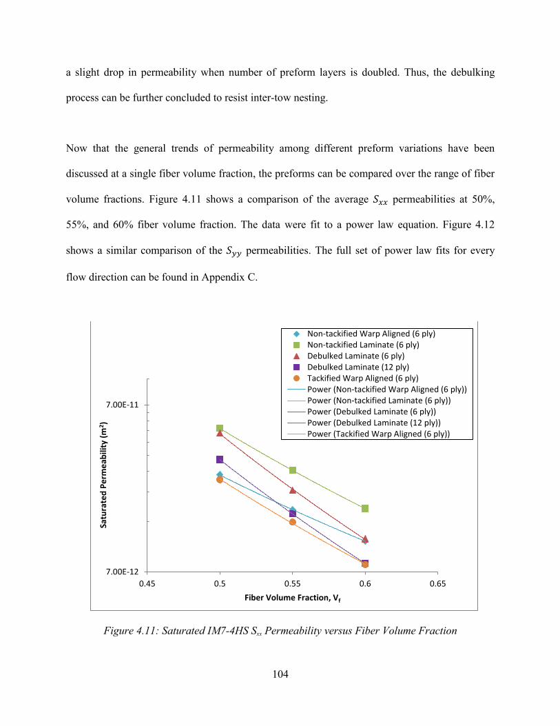
104
a slight drop in permeability when number of preform layers is doubled. Thus, the debulking
process can be further concluded to resist inter-tow nesting.
Now that the general trends of permeability among different preform variations have been
discussed at a single fiber volume fraction, the preforms can be compared over the range of fiber
volume fractions. Figure 4.11 shows a comparison of the average 𝑆𝑥𝑥 permeabilities at 50%,
55%, and 60% fiber volume fraction. The data were fit to a power law equation. Figure 4.12
shows a similar comparison of the 𝑆𝑦𝑦 permeabilities. The full set of power law fits for every
flow direction can be found in Appendix C.
Figure 4.11: Saturated IM7-4HS Sxx Permeability versus Fiber Volume Fraction
7.00E-12
7.00E-11
0.45 0.5 0.55 0.6 0.65
Satu
rate
d P
erm
eab
ility
(m
2 )
Fiber Volume Fraction, Vf
Non-tackified Warp Aligned (6 ply)Non-tackified Laminate (6 ply)Debulked Laminate (6 ply)Debulked Laminate (12 ply)Tackified Warp Aligned (6 ply)Power (Non-tackified Warp Aligned (6 ply))Power (Non-tackified Laminate (6 ply))Power (Debulked Laminate (6 ply))Power (Debulked Laminate (12 ply))Power (Tackified Warp Aligned (6 ply))
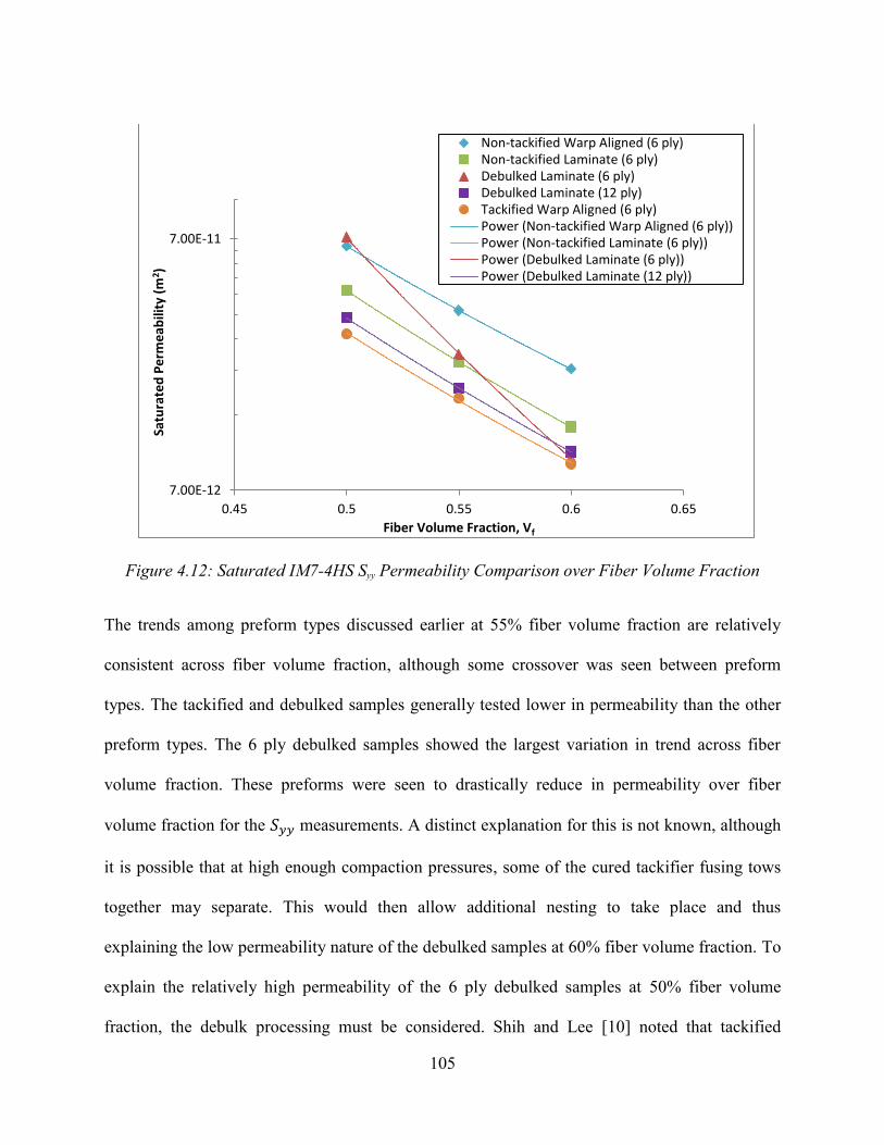
105
Figure 4.12: Saturated IM7-4HS Syy Permeability Comparison over Fiber Volume Fraction
The trends among preform types discussed earlier at 55% fiber volume fraction are relatively
consistent across fiber volume fraction, although some crossover was seen between preform
types. The tackified and debulked samples generally tested lower in permeability than the other
preform types. The 6 ply debulked samples showed the largest variation in trend across fiber
volume fraction. These preforms were seen to drastically reduce in permeability over fiber
volume fraction for the 𝑆𝑦𝑦 measurements. A distinct explanation for this is not known, although
it is possible that at high enough compaction pressures, some of the cured tackifier fusing tows
together may separate. This would then allow additional nesting to take place and thus
explaining the low permeability nature of the debulked samples at 60% fiber volume fraction. To
explain the relatively high permeability of the 6 ply debulked samples at 50% fiber volume
fraction, the debulk processing must be considered. Shih and Lee [10] noted that tackified
7.00E-12
7.00E-11
0.45 0.5 0.55 0.6 0.65
Satu
rate
d P
erm
eab
ility
(m
2 )
Fiber Volume Fraction, Vf
Non-tackified Warp Aligned (6 ply)Non-tackified Laminate (6 ply)Debulked Laminate (6 ply)Debulked Laminate (12 ply)Tackified Warp Aligned (6 ply)Power (Non-tackified Warp Aligned (6 ply))Power (Non-tackified Laminate (6 ply))Power (Debulked Laminate (6 ply))Power (Debulked Laminate (12 ply))

106
preforms should be compressed to a thickness slightly larger than the target thickness for a
permeability test, so the sample can be re-compressed to the desired fiber volume fraction in the
measurement fixture to avoid race-tracking over or under the sample. In the vacuum debulk
process, the vacuum pressure compacted the 6 ply preforms to a thickness very close or past the
50% fiber volume fraction point. This may allow for some race-tracking over the sample to take
place and artificially raise the permeability if the pre-compacted sample was of smaller thickness
than the cavity depth set in the permeability fixture. From the compaction experiments in
Chapter 3, it was observed that compacting the 6 ply debulked samples to 100 kPa (roughly full
vacuum pressure) produced fiber volume fractions just over 50%. Therefore, it may be possible
to observe race tracking effects with these samples at the 50% fiber volume fraction thickness set
in the permeability measurement cavity. In this case, the saturated permeability testing cavity
may be of slightly larger thickness than the sample, allowing the fluid a path of low resistance
over the top of the preform. Alternatively, the 12 ply debulked samples showed no artificially
high permeability at 50% fiber volume fraction, which corresponds to the trend of more
compaction resistance seen in these samples than in the 6 ply preforms in the Chapter 3 results.
4.2.1.2 Principal Permeability Ratios and Orientation
In addition to calculating principal in-plane permeabilities from the tensor transformation, the
angle of first principal permeability orientation (𝛽) was also found. It was observed that
relatively small changes in permeability measurements resulted in large changes in the 𝛽 angle.
For example, using 𝑆𝑥𝑥, 𝑆𝑦𝑦, and 𝑆𝑥𝑥′ data for the 6 ply non-tackified laminate, employing a
15% change in the original 𝑆𝑥𝑥 value returned a change in the 𝛽 angle of 19° from the original
tensor transformation. This is disappointing as average experimental scatter among in-plane
107
permeability measurements was seen to be roughly 15% for the non-tackified laminate. This
15% change in 𝑆𝑥𝑥 also resulted in only a 10% change in the 𝑆11 and a 3% change in 𝑆22 value.
The 𝛽 angle then appears to be much more sensitive to experimental scatter than the principal
permeability. Furthermore, employing a 15% change to the 𝑆𝑦𝑦 value results in only a 1° change,
while a 15% change in 𝑆𝑥𝑥′ results in an extremely large alteration of 40° in 𝛽, all while the
principal permeabilities are lightly altered in regards to experimental scatter. Demaría et al. [153]
also reviewed how small variations in the measured channel flow permeability measurements
make a noticeable change on the angle 𝛽. Even a 5% change in 𝑆𝑥𝑥 permeability was noted to
cause up to a 13% change in 𝛽 by Weitzenböck et al. [61]. Due to this sensitivity, 𝛽 cannot be
confidently reported for the IM7-4HS preforms tested in the saturated permeability fixture. A
radial visualization technique was then required to quantify the orientation angle. This is
discussed in detail in Chapter 8.
In this case, a more practical approach to quantifying the permeability tensors’ directional biases
is through comparing permeability ratios. Here, the 𝑆𝑥𝑥/𝑆𝑦𝑦 and 𝑆11/𝑆22 ratios can quantify the
anisotropy of the permeability of each preform type measured. The 𝑆𝑥𝑥/𝑆𝑦𝑦 ratio is simply the
warp over weft permeability, while the 𝑆11/𝑆22 shows the maximum ratio of preform anisotropy.
When the ratios are close to 1, the in-plane permeability behavior should be close to isotropic.
The permeability ratios calculated from average permeabilities for all preforms measured can be
seen in Table 4.4. The ratios are displayed over the fiber volume fractions tested. Note that the
12 ply debulked preform was not tested in the 𝑆𝑥𝑥′ direction, so the principal permeability ratio
could not be calculated.
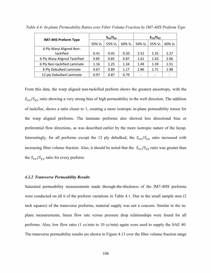
108
Table 4.4: In-plane Permeability Ratios over Fiber Volume Fraction by IM7-4HS Preform Type
IM7-4HS Preform Type Sxx/Syy S11/S22
50% Vf 55% Vf 60% Vf 50% Vf 55% Vf 60% Vf
6 Ply Warp Aligned Non-tackified 0.41 0.45 0.50 2.52 2.35 2.27
6 Ply Warp Aligned Tackified 0.85 0.85 0.87 1.61 1.63 2.06
6 Ply Non-tackified Laminate 1.16 1.25 1.34 1.49 1.39 1.51
6 Ply Debulked Laminate 0.67 0.89 1.17 2.86 1.71 1.98
12 ply Debulked Laminate 0.97 0.87 0.79 - - -
From this data, the warp aligned non-tackified preform shows the greatest anisotropy, with the
𝑆𝑥𝑥/𝑆𝑦𝑦 ratio showing a very strong bias of high permeability in the weft direction. The addition
of tackifier, shows a ratio closer to 1, creating a more isotropic in-plane permeability tensor for
the warp aligned preforms. The laminate preforms also showed less directional bias or
preferential flow directions, as was described earlier by the more isotropic nature of the layup.
Interestingly, for all preforms except the 12 ply debulked, the 𝑆𝑥𝑥/𝑆𝑦𝑦 ratio increased with
increasing fiber volume fraction. Also, it should be noted that the 𝑆11/𝑆22 ratio was greater than
the 𝑆𝑥𝑥/𝑆𝑦𝑦 ratio for every preform.
4.2.2 Transverse Permeability Results
Saturated permeability measurements made through-the-thickness of the IM7-4HS preforms
were conducted on all 6 of the preform variations in Table 4.1. Due to the small sample area (2
inch squares) of the transverse preforms, material supply was not a concern. Similar to the in-
plane measurements, linear flow rate versus pressure drop relationships were found for all
preforms. Also, low flow rates (1 cc/min to 10 cc/min) again were used to supply the SAE 40.
The transverse permeability results are shown in Figure 4.13 over the fiber volume fraction range
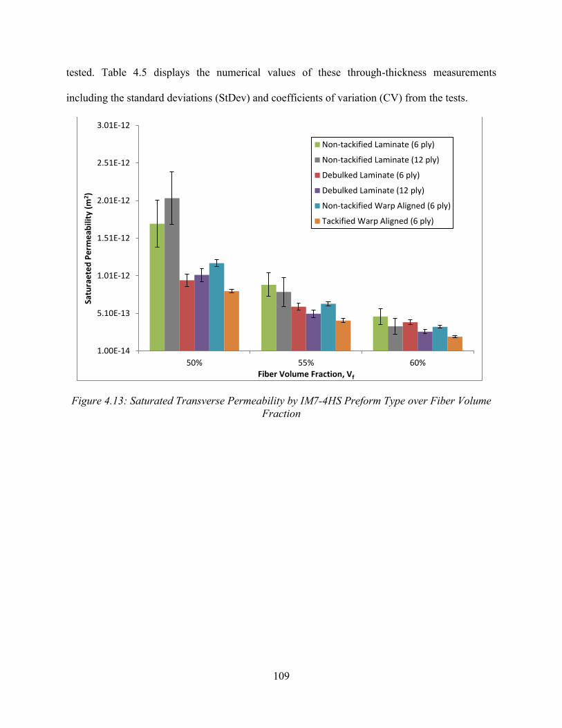
109
tested. Table 4.5 displays the numerical values of these through-thickness measurements
including the standard deviations (StDev) and coefficients of variation (CV) from the tests.
Figure 4.13: Saturated Transverse Permeability by IM7-4HS Preform Type over Fiber Volume Fraction
1.00E-14
5.10E-13
1.01E-12
1.51E-12
2.01E-12
2.51E-12
3.01E-12
50% 55% 60%
Satu
rae
ted
Pe
rme
abili
ty (
m2 )
Fiber Volume Fraction, Vf
Non-tackified Laminate (6 ply)
Non-tackified Laminate (12 ply)
Debulked Laminate (6 ply)
Debulked Laminate (12 ply)
Non-tackified Warp Aligned (6 ply)
Tackified Warp Aligned (6 ply)
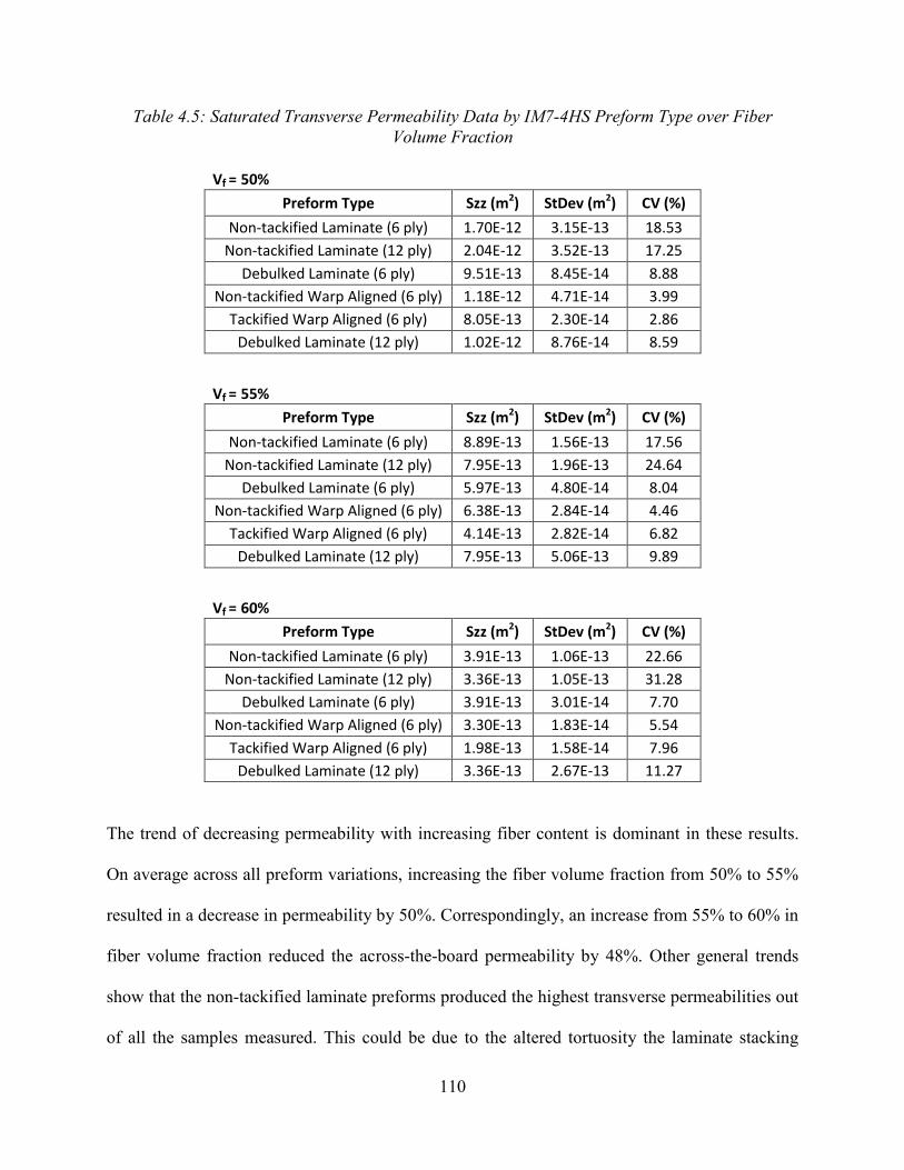
110
Table 4.5: Saturated Transverse Permeability Data by IM7-4HS Preform Type over Fiber Volume Fraction
Vf = 50% Preform Type Szz (m2) StDev (m2) CV (%)
Non-tackified Laminate (6 ply) 1.70E-12 3.15E-13 18.53
Non-tackified Laminate (12 ply) 2.04E-12 3.52E-13 17.25
Debulked Laminate (6 ply) 9.51E-13 8.45E-14 8.88
Non-tackified Warp Aligned (6 ply) 1.18E-12 4.71E-14 3.99
Tackified Warp Aligned (6 ply) 8.05E-13 2.30E-14 2.86
Debulked Laminate (12 ply) 1.02E-12 8.76E-14 8.59
Vf = 55% Preform Type Szz (m2) StDev (m2) CV (%)
Non-tackified Laminate (6 ply) 8.89E-13 1.56E-13 17.56
Non-tackified Laminate (12 ply) 7.95E-13 1.96E-13 24.64
Debulked Laminate (6 ply) 5.97E-13 4.80E-14 8.04
Non-tackified Warp Aligned (6 ply) 6.38E-13 2.84E-14 4.46
Tackified Warp Aligned (6 ply) 4.14E-13 2.82E-14 6.82
Debulked Laminate (12 ply) 7.95E-13 5.06E-13 9.89
Vf = 60% Preform Type Szz (m2) StDev (m2) CV (%)
Non-tackified Laminate (6 ply) 3.91E-13 1.06E-13 22.66
Non-tackified Laminate (12 ply) 3.36E-13 1.05E-13 31.28
Debulked Laminate (6 ply) 3.91E-13 3.01E-14 7.70
Non-tackified Warp Aligned (6 ply) 3.30E-13 1.83E-14 5.54
Tackified Warp Aligned (6 ply) 1.98E-13 1.58E-14 7.96
Debulked Laminate (12 ply) 3.36E-13 2.67E-13 11.27
The trend of decreasing permeability with increasing fiber content is dominant in these results.
On average across all preform variations, increasing the fiber volume fraction from 50% to 55%
resulted in a decrease in permeability by 50%. Correspondingly, an increase from 55% to 60% in
fiber volume fraction reduced the across-the-board permeability by 48%. Other general trends
show that the non-tackified laminate preforms produced the highest transverse permeabilities out
of all the samples measured. This could be due to the altered tortuosity the laminate stacking
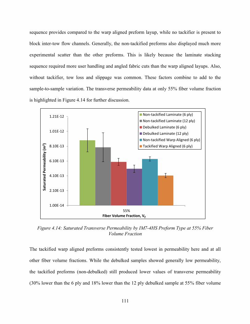
111
sequence provides compared to the warp aligned preform layup, while no tackifier is present to
block inter-tow flow channels. Generally, the non-tackified preforms also displayed much more
experimental scatter than the other preforms. This is likely because the laminate stacking
sequence required more user handling and angled fabric cuts than the warp aligned layups. Also,
without tackifier, tow loss and slippage was common. These factors combine to add to the
sample-to-sample variation. The transverse permeability data at only 55% fiber volume fraction
is highlighted in Figure 4.14 for further discussion.
Figure 4.14: Saturated Transverse Permeability by IM7-4HS Preform Type at 55% Fiber Volume Fraction
The tackified warp aligned preforms consistently tested lowest in permeability here and at all
other fiber volume fractions. While the debulked samples showed generally low permeability,
the tackified preforms (non-debulked) still produced lower values of transverse permeability
(30% lower than the 6 ply and 18% lower than the 12 ply debulked sample at 55% fiber volume
1.00E-14
2.10E-13
4.10E-13
6.10E-13
8.10E-13
1.01E-12
1.21E-12
55%
Satu
rate
d P
erm
eab
ility
(m
2 )
Fiber Volume Fraction, Vf
Non-tackified Laminate (6 ply)
Non-tackified Laminate (12 ply)
Debulked Laminate (6 ply)
Debulked Laminate (12 ply)
Non-tackified Warp Aligned (6 ply)
Tackified Warp Aligned (6 ply)

112
fraction). As described earlier in the in-plane permeability discussion, this is likely because the
tackifier aids in blocking the inter-tow flow channels, while still allowing nesting to take place
where the debulked samples resisted nesting.
Another important result to note is, as a whole, the through-thickness direction of the IM7-4HS
preforms was much less permeable than their in-plane counterparts. This is a trend that has been
cited and is well known for most reinforcements [60]. Transverse permeability has been reported
to be over two magnitudes lower than the in-plane permeabilities of the same preform [101].
Using sample data from the 6 ply non-tackified laminate permeability measurements, the two in-
plane principal permeabilities and the 𝑆𝑧𝑧, or effectively the 𝑆33, can be plotted across fiber
volume fraction on one plot. This is seen in Figure 4.15 where the permeability is plotted on a
logarithmic scale.
Figure 4.15: Principal Permeabilities over Fiber Volume Fraction for the 6 Ply Non-tackified Laminate IM7-4HS
1.00E-13
1.00E-12
1.00E-11
1.00E-10
0.45 0.5 0.55 0.6 0.65
Satu
rate
d P
erm
eab
ility
(m
2 )
Fiber Volume Fraction, Vf
S11
S22
S33
Power (S11)
Power (S22)
Power (S33)
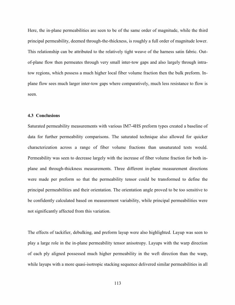
113
Here, the in-plane permeabilities are seen to be of the same order of magnitude, while the third
principal permeability, deemed through-the-thickness, is roughly a full order of magnitude lower.
This relationship can be attributed to the relatively tight weave of the harness satin fabric. Out-
of-plane flow then permeates through very small inter-tow gaps and also largely through intra-
tow regions, which possess a much higher local fiber volume fraction then the bulk preform. In-
plane flow sees much larger inter-tow gaps where comparatively, much less resistance to flow is
seen.
4.3 Conclusions
Saturated permeability measurements with various IM7-4HS preform types created a baseline of
data for further permeability comparisons. The saturated technique also allowed for quicker
characterization across a range of fiber volume fractions than unsaturated tests would.
Permeability was seen to decrease largely with the increase of fiber volume fraction for both in-
plane and through-thickness measurements. Three different in-plane measurement directions
were made per preform so that the permeability tensor could be transformed to define the
principal permeabilities and their orientation. The orientation angle proved to be too sensitive to
be confidently calculated based on measurement variability, while principal permeabilities were
not significantly affected from this variation.
The effects of tackifier, debulking, and preform layup were also highlighted. Layup was seen to
play a large role in the in-plane permeability tensor anisotropy. Layups with the warp direction
of each ply aligned possessed much higher permeability in the weft direction than the warp,
while layups with a more quasi-isotropic stacking sequence delivered similar permeabilities in all

114
test directions. The presence of inter-layer tackifier was seen to reduce permeability in all test
directions due to a blocking of inter-tow gaps, while some directions were more affected than
others. Tackified samples in the warp aligned preforms created a much more isotropic in-plane
permeability tensor compared to the non-tackified. Debulked samples proved to be most difficult
to characterize in permeability. The curing of the tackifier altered the compaction behavior of
these samples. Debulked samples resisted inter-ply nesting, and resulted in higher permeability
than the tackified, non-debulked samples as fewer inter-tow flow channels were blocked.
Transverse measurements showed similar trends, while permeability here was roughly an order
of magnitude lower than in the in-plane measurements.
Using the produced permeability data here, Darcian flow based process models can be created to
simulate mold fills for RTM. If low permeability is not a concern, tackified IM7-4HS should be
used in a manufacturing setting over the non-tackified material, as the tackifier aids in holding
fiber orientation and preform shape. Debulking will further hold preform shape, although
preform compaction and race-tracking may become a concern inside the mold. Note that the
injected resin should be compatible with tackifier used in preforming. Future work for a more
robust characterization could include the effect of shear and flow through curved portions of the
reinforcement. Further work could develop an in situ permeability measurement system, where
the effects of the unique geometrical features of specific molds could be characterized before
infusion.

115
5. Fluid Effects
Understanding how reinforcement fibers interact with a permeating fluid is telling to the degree
of compatibility between the reinforcement and matrix. In this study, the majority of
permeability measurements was made with SAE 40 motor oil due to the low cost and ease of use
with respect to equipment cleanup. For actual LCM infusions, epoxy resins are used that possess
different surface chemistry than that of motor oil. Due to differing surface chemistry, the
adhesion between the reinforcing fibers and the fluids could be affected. Wettability of the fibers
may be altered and a natural inquiry asks if the fluid type affects permeability. As stated in the
literature review, the effect of fluid type on permeability has been controversial. Some
researchers have found little effect compared to experimental scatter [115], [116], while others
found large deviations based on the fluid used [117]. To investigate this fiber/fluid interaction
and compare different fluids, measurements of the liquid to fiber contact angle and fluid surface
tension can be made. Low contact angles and surface tensions are generally desired for LCM.
Lower contact angles promote better fiber wet out while lower fluid surface tensions leads to
better adhesion and ultimately fewer voids in the finished part [43]. Contact angle and surface
tension measurements can then be implemented to define capillary pressure and a capillary
number for unsaturated infusions.
To investigate the fluid type effects on permeability, SAE 40 motor oil was compared to Applied
Poleramic’s SC-15 epoxy resin system (a VARTM resin with similar viscosity to that of the oil
at room temperature) in unsaturated, one-dimensional flow experiments. The resin system, SC-

116
15, has an epoxy component, Part A, and an amine hardening component, Part B (mixing ratio of
Part A:Part B = 100:30). A basic comparison of the fluids’ properties can be seen in Table 5.1.
Table 5.1: Basic Properties of Test Fluids
Fluid SAE 40 Oil SC-15 Part A
(Resin) SC-15 Part B (Hardener)
SC-15 Mixed (A:B = 100:30)
Viscosity at Ambient (Pa-s)
0.24 0.58 0.045 0.285
Density at Ambient (kg/m^3)
706 1129 961 1085
A direct comparison of permeability produced from SAE 40 oil infusions and permeability
produced from SC-15 infusions is made for IM7-4HS preforms with and without the inter-layer
tackifier. Both the epoxy and motor oil were also measured for surface tension and contact angle
with IM7. This first half of this chapter discusses the experimental approach and results of fluid
surface tension and fiber contact angle measurements. The second half of the chapter introduces
the unsaturated permeability measurement technique and discusses capillary effects on
permeability induced from the interactions characterized in the first half.
5.1 Contact Angle and Surface Tension Measurements
5.1.1 Methods
5.1.1.1 Surface Tension Measurements
To measure fluid surface tensions of the SAE 40 oil and epoxy portion of the SC-15, the Du
Noüy ring method was employed. With this measurement technique, a platinum-iridium ring of
known surface contact angle is introduced into a test fluid with unknown surface tension. The Du
Noüy ring method was carried out on a Thermo Cahn Dynamic Contact Angle (DCA) analyzer
model 322, seen in Figure 5.1. The DCA possesses a high-precision balance with sensitivity
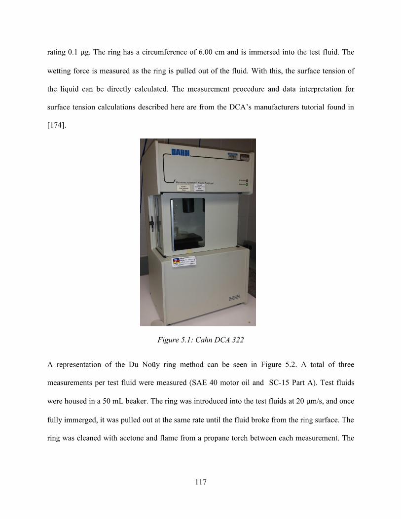
117
rating 0.1 µg. The ring has a circumference of 6.00 cm and is immersed into the test fluid. The
wetting force is measured as the ring is pulled out of the fluid. With this, the surface tension of
the liquid can be directly calculated. The measurement procedure and data interpretation for
surface tension calculations described here are from the DCA’s manufacturers tutorial found in
[174].
Figure 5.1: Cahn DCA 322
A representation of the Du Noüy ring method can be seen in Figure 5.2. A total of three
measurements per test fluid were measured (SAE 40 motor oil and SC-15 Part A). Test fluids
were housed in a 50 mL beaker. The ring was introduced into the test fluids at 20 µm/s, and once
fully immerged, it was pulled out at the same rate until the fluid broke from the ring surface. The
ring was cleaned with acetone and flame from a propane torch between each measurement. The

118
ring was allowed to fully cool to room temperature before subsequent testing. Also, between
each measurement of the same liquid, a fresh liquid surface was introduced by pipet injection.
Figure 5.2: Du Noüy Ring Representation
Using the relation seen in Equation 56, the surface tension of the fluid, 𝜎, can then be determined
where 𝜎′ is the raw surface tension reading from the wetting force measurement and 𝑐𝑓 is the
correction factor
𝜎 = 𝜎′𝑐𝑓 (56)
The raw surface tension is then defined as
𝜎′ =
𝐹𝑤𝑝
(57)
Test Fluid
Glass Beaker
Du Noüy Ring

119
Here, 𝐹𝑤 is the measured wetting force during the ring pullout and 𝑝 is the wetted perimeter
(𝑝 = 4𝜋𝑅 where 𝑅 is the radius of the ring). As recommended from the DCA manufacturer
[174], the Deutsches Institut für Normung (DIN) standard of using the max pull point (point of
maximum wetting force during ring pullout) for the surface tension calculation was used rather
than the American Society for Testing and Materials (ASTM) standard of using the break point.
The break point (the point during the test at which the fluid breaks away from the Du Noüy ring
as it is pulled from the fluid) may be altered from vibrations or other outside interferences [175].
The correction factor is used to account for the liquid that is attached to the bottom of the Du
Noüy ring during pullout. The correction factor is defined in Equation 58, where 𝐶 is the mean
circumference of the ring, 𝜌𝑓𝑙𝑢𝑖𝑑 is the density of the test fluid, 𝜌𝑎𝑖𝑟 is the density of the
surrounding air, 𝑅 is the radius of the ring, and 𝑟 is the radius of the wire composing the Du
Noüy ring. The density of the oil was provided by the manufacturer, while the density of the
epoxy was referenced from the resin system material data sheet in [176].
𝑐𝑓 = 0.7250 + √
1.452𝜎′
𝐶2(𝜌𝑓𝑙𝑢𝑖𝑑 − 𝜌𝑎𝑖𝑟)+ 0.04534 −
1.679
𝑅/𝑟 (58)
5.1.1.2 Contact Angle Measurements
To measure the advancing and receding contact angles of the SAE 40 motor oil and epoxy resin
on the IM7 carbon fibers, the micro-Wilhelmy method was used. This method is similar to the
Du Noüy ring method as it also employs the Cahn DCA, although single carbon fibers, attached
to wire hangers, are introduced into the test fluid. A representation of the micro-Wilhelmy setup
using the Cahn DCA 322 can be seen in Figure 5.3.

120
Figure 5.3: Micro-Wilhelmy Setup using the Thermo Cahn DCA 322
Using the relation in Equation 59, the advancing and receding fiber contact angles, 𝜃, can be
determined for each test fluid.
cos 𝜃 =
𝐹𝑤𝜎𝑝
(59)
The wetted perimeter, 𝑝, in this case refers to the fiber’s circumference, while 𝜃 is the fiber
contact angle, and 𝐹𝑤 is the measured wetting force. Also, the work of adhesion between fiber
and liquid can be determined from these measurements. The work of adhesion is defined as the
total attraction between two phases, and is produced from both chemical and physical factors
[177]. The work of adhesion, 𝑊𝐴, can be calculated from the measured quantities of fluid surface
tension and contact angle as seen in Equation 60 [177], [178].
𝑊𝐴 = 𝜎(1 + cos 𝜃) (60)
To obtain these wetting force measurements, micro-Wilhelmy samples were first laid up. To
assemble the fiber samples, single carbon fibers were selected from a tow of the IM7-4HS fabric.
Sample Loops
Balance System
Wire Sample Hanger
Fiber Sample
Counter-weight Loop
Test Fluid
Fluid Container
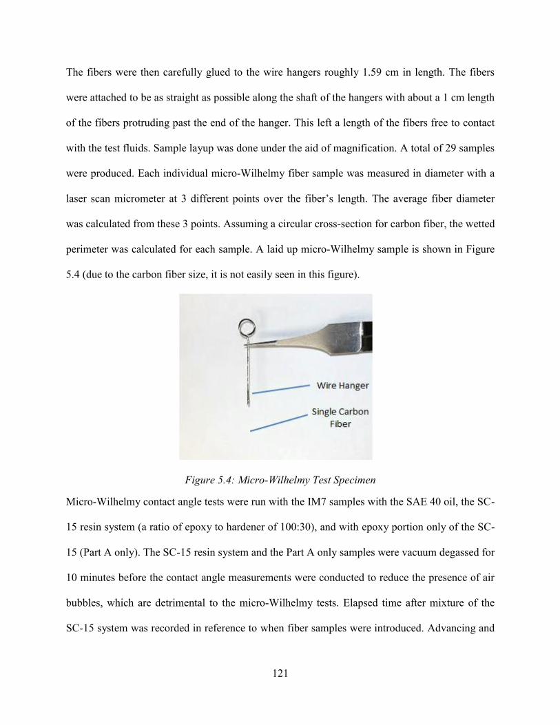
121
The fibers were then carefully glued to the wire hangers roughly 1.59 cm in length. The fibers
were attached to be as straight as possible along the shaft of the hangers with about a 1 cm length
of the fibers protruding past the end of the hanger. This left a length of the fibers free to contact
with the test fluids. Sample layup was done under the aid of magnification. A total of 29 samples
were produced. Each individual micro-Wilhelmy fiber sample was measured in diameter with a
laser scan micrometer at 3 different points over the fiber’s length. The average fiber diameter
was calculated from these 3 points. Assuming a circular cross-section for carbon fiber, the wetted
perimeter was calculated for each sample. A laid up micro-Wilhelmy sample is shown in Figure
5.4 (due to the carbon fiber size, it is not easily seen in this figure).
Figure 5.4: Micro-Wilhelmy Test Specimen
Micro-Wilhelmy contact angle tests were run with the IM7 samples with the SAE 40 oil, the SC-
15 resin system (a ratio of epoxy to hardener of 100:30), and with epoxy portion only of the SC-
15 (Part A only). The SC-15 resin system and the Part A only samples were vacuum degassed for
10 minutes before the contact angle measurements were conducted to reduce the presence of air
bubbles, which are detrimental to the micro-Wilhelmy tests. Elapsed time after mixture of the
SC-15 system was recorded in reference to when fiber samples were introduced. Advancing and

122
receding contact angles were found by introducing the fibers into the test fluids at 20 µm/s to an
immersion depth of 3 mm, and then allowed to recede at the same speed until the fibers were
pulled out of the liquid. The test fluids were housed in 10 mL glass beakers during these
measurements. The wetting force during advancement and recession of the fibers were recorded
from the DCA high precision balance and were used to find the contact angles. To do this, the
advancing and receding portions of the curve were fit separately to linear regressions to account
for the buoyancy effect. The advancing and receding wetting forces were then solved from these
regressions at the point of zero depth of immersion (ZDOI) and used for the contact angle
calculation.
5.1.2 Results and Discussion
5.1.2.1 Surface Tension Measurements
A total of 3 surface tension calculations were made for each test fluid using the Du Noüy ring
method. Surface tension tests were made after the fiber contact angle measurements, and due to
unsuccessful micro-Wilhelmy measurements with the full SC-15 system (Part A and Part B),
only the epoxy portion (Part A) of the SC-15 and the SAE 40 motor oil and were measured. The
surface tension calculations from each run of both tested liquids are listed in Table 5.2 along
with the average, standard deviation (StDev), and percent coefficient of variation (CV). Note that
the surface tension measurements for both fluids were made at room temperature in air.

123
Table 5.2: Surface Tension Measurement Results by Test Fluid
Surface Tension by Test Fluid (dyne/cm)
Run # SAE 40 Motor Oil SC-15 Part A
1 29.18 32.36
2 29.12 32.41
3 29.14 32.46
Average 29.15 32.41
StDev 0.03 0.05
CV (%) 0.11 0.16
The surface tension results were very consistent for both fluids as seen in the table. Also, both
the epoxy and motor oil were measured to possess a very similar surface tension value. Due to
the small difference between surface tensions of the motor oil and epoxy, it is difficult to make
an inference towards the determination of a better wetting fluid. Contact angle and work of
adhesion results will aid in this. Literature values for the SC-15 epoxy could not be found for a
comparison. The SAE 40 motor oil compares close to reported value of 35 dyne/cm for SAE 30
and SAE 50 oils [179]. A full list of surface tension measurement run data, including values for
raw measurement surface tension, correction factors, and maximum pull out weights can be
found in Appendix B. Also, sample wetting force graphs for both oil and epoxy in the Du Noüy
ring measurements can be found in Appendix B.
5.1.2.2 Fiber Diameter Measurements
Of the 29 micro-Wilhelmy fiber samples measured, the average diameter of one sample was
significantly higher than the remaining samples, so it was concluded that this was actually 2
fibers still twisted together from the tow. That left 28 samples of single fibers diameters. Each

124
fiber diameter was averaged over three points. The average IM7 fiber diameter, perimeter,
standard deviation (StDev) and coefficient of variation (CV) are listed in Table 5.3.
Table 5.3: IM7 Fiber Diameter Statistics
Average Data from 28 Fiber Samples
Fiber Diameter (µm) 5.59
Diameter StDev (µm) 0.27
Diameter CV (%) 4.86
Fiber Perimeter (From Average) (µm) 17.55
Compared to the manufacturer’s supplied average fiber diameter of 5.2 µm shown in Table 1.1,
the experimental average was about 7% higher. It should be noted that the sample body average
diameter was not used for each contact angle measurement. Each individual fiber diameter was
used for more accuracy. The entire data sample set can be seen in Appendix B.
5.1.2.3 Contact Angle Measurements
During micro-Wilhelmy testing for fiber contact angles, 13 IM7 fiber samples were designated
for tests with the oil, 8 samples were designated for the SC-15 resin system, and 8 samples were
designated for SC-15 Part A measurements. Due to fiber irregularities, bubbles in test fluids, and
other effects, not all samples test data was used. Also, for some samples, only the advancing
contact angle data was produced. A full list of the micro-Wilhelmy fibers and their data status
can be found in Appendix B. Successful measurements were taken from 10 out of the 13 fiber
samples used with the oil, all 8 fibers samples used with the SC-15 Part A, and none of the 8
samples measured with the full SC-15 system produced usable data for advancing contact angles.
The advancing and receding contact angle results can be seen in Table 5.4. A complete list of
individual fibers and their test data can be found in Appendix B.
125
Table 5.4: Advancing and Receding Contact Angle Measurement Results by Fluid
Fluid SAE 40 Oil SC-15 Part A (Epoxy only)
Contact Angle Type Advancing Receding Advancing Receding
Sample Size 10 9 8 7
Average θ (degrees)
45.34 56.36 37.54 47.81
StDev θ (degrees) 5.92 3.96 5.63 6.91
CV (%) 13.06 7.03 14.99 14.46
These results infer that the epoxy is a better wetting liquid with the IM7 fiber because the
advancing contact angle is smaller than that of the oil. While this comparison has been made by
some researchers [43] to indicate a better wetting fluid, Miller [177] argues that only in a
comparison of a single fluid does an increase in attraction confidently result in a decrease in
contact angle. Therefore, the work of adhesion should be examined. While the epoxy possesses
a lower average contact angle, both sets of fluid produced advancing contact angles with
standard deviations of about 6 degrees. With this variation and a difference between the fluids
averages of about 7 degrees, the difference of wettability between the fluids may not be
statistically relevant. Other results show that the advancing contact angles for both fluids is less
than their receding counterparts implying that a dry fiber is more attracted to the test fluids than a
pre-wetted fiber. The calculated work of adhesion for these fluids with the IM7 will further
investigate these inferences.
The work of adhesion for both advancement and recession were calculated for the motor oil and
epoxy. The results are displayed in Table 5.4. This table also includes values of a hysteresis ratio,
which is the ratio of between the work of adhesion of advancement over recession (hysteresis
ratio= 𝑊𝐴𝑟/𝑊𝐴
𝑎). This was done for each full micro-Wilhelmy measurement (including both
advancing and receding portions of the wetting force curve). The hysteresis ratio is clear
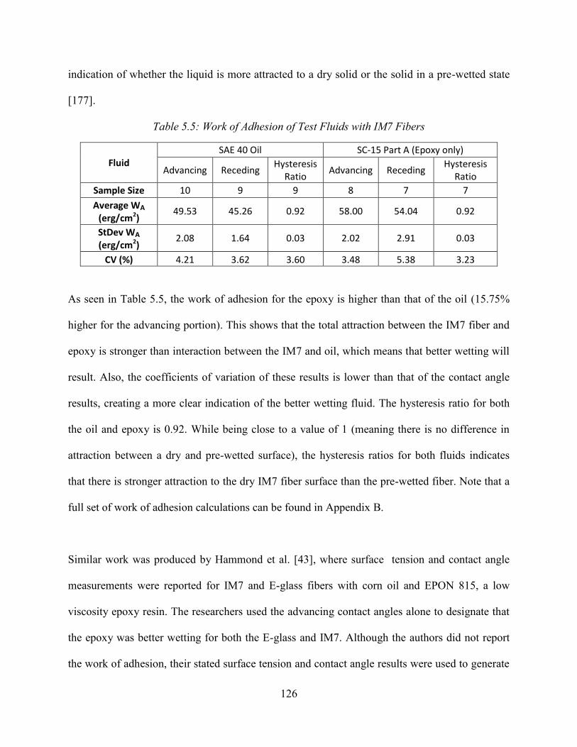
126
indication of whether the liquid is more attracted to a dry solid or the solid in a pre-wetted state
[177].
Table 5.5: Work of Adhesion of Test Fluids with IM7 Fibers
Fluid SAE 40 Oil SC-15 Part A (Epoxy only)
Advancing Receding Hysteresis
Ratio Advancing Receding
Hysteresis Ratio
Sample Size 10 9 9 8 7 7
Average WA (erg/cm2)
49.53 45.26 0.92 58.00 54.04 0.92
StDev WA (erg/cm2)
2.08 1.64 0.03 2.02 2.91 0.03
CV (%) 4.21 3.62 3.60 3.48 5.38 3.23
As seen in Table 5.5, the work of adhesion for the epoxy is higher than that of the oil (15.75%
higher for the advancing portion). This shows that the total attraction between the IM7 fiber and
epoxy is stronger than interaction between the IM7 and oil, which means that better wetting will
result. Also, the coefficients of variation of these results is lower than that of the contact angle
results, creating a more clear indication of the better wetting fluid. The hysteresis ratio for both
the oil and epoxy is 0.92. While being close to a value of 1 (meaning there is no difference in
attraction between a dry and pre-wetted surface), the hysteresis ratios for both fluids indicates
that there is stronger attraction to the dry IM7 fiber surface than the pre-wetted fiber. Note that a
full set of work of adhesion calculations can be found in Appendix B.
Similar work was produced by Hammond et al. [43], where surface tension and contact angle
measurements were reported for IM7 and E-glass fibers with corn oil and EPON 815, a low
viscosity epoxy resin. The researchers used the advancing contact angles alone to designate that
the epoxy was better wetting for both the E-glass and IM7. Although the authors did not report
the work of adhesion, their stated surface tension and contact angle results were used to generate

127
the data in Table 5.6. The fluid and fiber results are compared here with the IM7 fiber results
from this current study. Note that the IM7 fibers from Hammond et al. [43] were from a 8-
harness satin weave fabric, and due to possible differences with surface treatments, sizing, or
other manufacturing variables, these results cannot be compared to the current study in a direct,
quantitative sense, although the general trends of the comparison are relevant.
Table 5.6: Fluid Surface Tension, Contact Angle and Work of Adhesion Comparison with Hammond et al. [43] for IM7 Fibers
Current Study Results
Results from Hammond et al. [43]
Fluid SAE 40 Oil SC-15 Part A (Epoxy only)
Corn Oil EPON 815
Surface Tension (dyne/cm)
29.1 32.4 26.5 37.2
Average Advancing θ (degrees)
45.3 37.5 36.1 28.5
Advancing WA (erg/cm2) 49.5 58.0 48.0 69.9
The comparison between these results is strikingly similar. Both results indicate that the epoxy
was better wetting than their oil counterparts through lower contact angles and higher work of
adhesion. Also, in both sets of results, the epoxy possessed higher surface tension than its oil
equivalent. Overall, it can be concluded that the SC-15 epoxy is a better wetting fluid than the
SAE 40 oil, while these similar results in literature [43] have produced concurring testimony.
Regarding the results of the SC-15 Part A and Part B mixture, the likely causes of the low
success rate of the micro-Wilhelmy measurements could be due to air bubbles present after
degassing and the chemical reactions taking place. Even after degassing, some air was still
entrapped in the SC-15. Since the resin surface properties were time sensitive, extended

128
degassing cycles were not pursued. Also, upon placement of the resin supply in the DCA
measurement chamber, a thin film or skin would start to form on the surface of resin (in a matter
of minutes) due to the interaction with the atmosphere. This skin would cause the fiber samples
to bend upon contact and ruin sampling data. To prevent this, the surface film was manually
broken up with a sterile glass pipet, although the complete elimination of these highly viscous
formations could not be confirmed before each test. It should be noted that the low success rate
of the contact angle measurements made with the SC-15 Part A and Part B system are due to the
fluid rather than fiber inconsistencies.
A sample graph of fiber contact angle measurement data is shown in Figure 5.5 displaying the
wetting force being tracked as a function of the fiber immersion depth. This sample was
immersed in SC-15 Part A. The significant features of the immersion and recession curve are
noted in the figure. Fiber surface irregularities also can be seen on the advancing portion of the
curve. The following graph in Figure 5.6 displays the advancing and receding portion of the
wetting force transient. These curve potions were fitted to linear regressions. The fitted points at
zero depth of immersion (ZDOI) are also marked, which are used for the fiber contact angle
calculations to account for the buoyancy effect as described earlier.
Fiber irregularities are also found as spikes in the wetting force curve [180] as seen in Figure 5.7.
Tests that produced unusable data show results typical to those in Figure 5.8. Throughout testing,
the IM7 fiber samples produced moderately consistent wetting force readouts, which correlate to
a fairly smooth surface. This smoothness could be a product of the sizing or surface treatment
placed on the fibers by the fabric manufacturer. Hammond et al. [43] also mentioned this

129
regarding the apparent smoothness of their IM7 fibers seen in scanning electron micrographs.
Irregularities in the form of spikes on the advancing and receding curves were excluded in the
buoyancy correction linear regressions. Some of the irregularities could be due to fiber sizing
inconsistencies or from deformations experienced when the fibers were manually separated from
the tow.
Figure 5.5: Sample Micro-Wilhelmy Test Data
-0.01
0
0.01
0.02
0.03
0.04
0.05
0.06
0.07
0 0.5 1 1.5 2 2.5 3 3.5 4 4.5 5
We
ttin
g Fo
rce
(m
g)
Fiber Immersion Depth (mm)
Transient Wetting Force
Fiber above fluid
Fiber advancing in fluid
Fiber receding in fluid
Fiber surface irregularities
Fiber tip artifact
ZDOI

130
Figure 5.6: Sample Micro-Wilhelmy Test Data with Buoyancy Correction
Figure 5.7: Sample Micro-Wilhelmy Test Data
y = -0.0014x + 0.0379
y = 0.0011x + 0.0450
-0.01
0
0.01
0.02
0.03
0.04
0.05
0.06
0.07
0 0.5 1 1.5 2 2.5 3 3.5 4 4.5 5
We
ttin
g Fo
rce
(m
g)
Fiber Immersion Depth (mm)
Transient Wetting Force
Advance
Recede
-0.01
0
0.01
0.02
0.03
0.04
0.05
0.06
0.07
0 0.5 1 1.5 2 2.5 3 3.5 4 4.5 5
We
ttin
g Fo
rce
(m
g)
Fiber Immersion Depth (mm)
Transient Wetting Force
Fiber surface irregularity
ZDOI
Buoyancy Corrected Wetting Force Measurement Points

131
Figure 5.8: Sample Micro-Wilhelmy Unusable Test Data
From the results of fluid and fiber interactions, it was then necessary to determine if these fluid
properties would produce significant effects in the determination of experimental preform
permeability. To do this, the surface tension and contact angle results were used to quantify
capillary effects and direct comparisons of SC-15 epoxy and SAE 40 motor oil infusions were
made. This work will be discussed in detail in the next section of this chapter.
-0.01
0.01
0.03
0.05
0.07
0.09
0.11
0.13
0.15
0 0.5 1 1.5 2 2.5 3 3.5 4 4.5 5 5.5
We
ttin
g Fo
rce
(m
g)
Fiber Immersion Depth (mm)
Transient Wetting Force
132
5.2 Unsaturated Channel Flow Measurements with Differing Fluids
5.2.1 Methods
5.2.1.1 Experimental Setup
Advancing front permeability measurements for both SAE 40 oil and SC-15 Part A were
obtained using a channel flow visualization fixture. The full SC-15 resin system (Part A and B
mixture) was not used here due to the unsuccessful micro-Wilhelmy characterization discussed
earlier. This permeability fixture provided the ability to visually observe flow fronts progressing
through preforms of IM7-4HS. The fixture is constructed of aluminum and allows a preform
15.13 cm in width, 17.11 cm in length, and 6.35 cm in thickness. A line source and line sink lay
on either side of the fixture’s preform cavity, which produces a rectilinear, in-plane flow. An
Airtech pressure pot was used to supply constant pressure injections of the test fluids with the aid
of a pressure regulator. The fixture was outfitted with an Omega PX-180 in-line pressure
transducer, which monitored the precise supplied injection pressure. Using a camera positioned
over the visualization window, advancing flow front locations were recorded while the elapsed
time was monitored with a stopwatch. An exploded view schematic of the fixture can be seen in
Figure 5.9.

133
Figure 5.9: Exploded View Schematic of the Channel Flow Unsaturated Permeability Fixture
The channel flow fixture has two visualization windows, one on the top and one oriented on the
side to allow for viewing the preform’s cross-section. Due to the dark color of the IM7-4HS
preforms, only the flow front view through the top visualization window was recorded by the
camera and clear differentiation could be made between saturated and unsaturated regions of the
reinforcement.
The nature of advancing front permeability measurements restricts the number of permeability
data points to one per preform. As opposed to saturated measurements, permeability at only one
fiber volume fraction can be calculated in unsaturated experiments. Once a preform is saturated
in an advancing front test, it cannot be measured again under the same conditions. Due to this
limitation, IM7-4HS preforms of a single layup, fiber volume fraction, and flow direction were
tested in order to maximize material supply. The focus of the unsaturated permeability
experiments were to determine the effects of capillary pressure, fluid type, tackifier, and
injection pressure on permeability. This means that layup orientation and ply number effects
Fixture Cavity
Preform
Fixture Top Half
Visualization Window
Fluid Inlet
Fluid Outlet
Inlet Pressure Transducer
Securing Bolts

134
were not investigated as they were studied in the saturated experiments. Two aluminum shims
were carefully cut and sealed with silicone into the unsaturated test fixture to produce a cavity
depth of 1.68 mm, resulting in an IM7-4HS preform fiber volume fraction of 54.6% with 8 plies.
A warp direction aligned preform layup was used for each sample producing a stacking sequence
of [0]8. Multiple measurements were made at 69, 138 and 276 kPa (10, 20 and 40 psi) target
constant inlet pressure set points. These unsaturated test parameters and others can be seen in
Table 5.7.
Table 5.7: Unsaturated Channel Flow Test Setup Parameters
Material Layup Vf Constant Inlet Pressures Set Points (kPa)
# Runs per Inlet Pressure
Set Point
Flow Direction
Non-tackified IM7-4HS [0]8 54.6% 69, 138, 276 3 Warp or Sxx
Tackified IM7-4HS [0]8 54.6% 69, 138, 276 3 Warp or Sxx
Each infusion experiment was recorded and post-processed to determine the unsaturated,
advancing front permeability. The visualization fixture window was graduated every 6.35 mm
(0.5 inch) so that location and time of the flow front was easily distinguished at these points. The
flow front locations were recorded over time and the method described by Hammond et al. [43]
was used to derive the permeability. Beginning with Darcy’s law of form in Equation 61,
substitutions of 𝑄𝐴=
𝑑𝑥
𝑑𝑡𝜑 and 𝑑𝑃
𝑑𝑥= −
∆𝑃
𝑥 can be made to derive an altered form of Darcy’s law in
Equation 62. Recall that in Darcy’s law, 𝑄 is the flow rate, 𝐴 is the cross-sectional area normal to
flow, 𝜇 is the fluid viscosity, 𝑆 is the permeability, and 𝑑𝑃𝑑𝑥
is the pressure gradient.
𝑄
𝐴= −
𝑆
𝜇
𝑑𝑃
𝑑𝑥 (61)
𝑑𝑥
𝑑𝑡𝜑 =
𝑆
𝜇
∆𝑃
𝑥 (62)

135
Here, ∆𝑃 is the pressure drop over the preform length, or essentially the injection pressure if
gage pressure is used, 𝜑 is the preform porosity, and 𝑡 is the time elapsed at the flow front
location, 𝑥. Then, by integrating Equation 62 with an initial condition of 𝑥(0) = 0, one can
derive the relationship seen in Equation 63.
𝑥2 = (
2𝑆∆𝑃
𝜇𝜑) 𝑡 (63)
By using a linear pressure drop versus flow front location assumption, the measured flow front
location squared (𝑥2) versus time can be fit to a linear regression where (2𝑆∆𝑃𝜇𝜑
) is the slope (say,
𝑚, with units of length squared per second) of the experimental data. Then, the unsaturated
permeability of the preform can be determined directly from the slope of the 𝑥2 verses time
curve with Equation 64. Note that this derives average unsaturated preform permeability over the
infusion by taking the slope of all experimental points on the curve.
𝑆𝑢𝑛𝑠𝑎𝑡 =
𝑚𝜇𝜑
2∆𝑃 (64)
The linear pressure drop assumption is valid if a good linear regression fit can be made for the
experimental flow front location squared versus time data. If this is not the case, then the
assumption cannot be used and permeability must be calculated separately per flow front
location or time of interest.
5.2.1.2 Capillary Pressure Determination
If capillary pressure is to be accounted for during the calculation of experimental unsaturated
permeability, then this value can be added with the injection or mechanical pressure term [123],
[133]. This gives

136
∆𝑃 = 𝑃𝑖𝑛𝑗 + 𝑃𝑐 (65)
Here, 𝑃𝑖𝑛𝑗 is the constant injection pressure of the infusion and 𝑃𝑐 is the capillary pressure. Note
that this formulation neglects gravitational pressure, which is assumed to have little influence on
the entire pressure drop. This pressure drop can then be directly substituted back into Equation
63 and Equation 64. To define the capillary pressure, experimental or theoretical techniques can
be used. In this study, analytical formulations will be used to define capillary pressure
contributions, as well as, an experimental technique based on constant injection pressure
infusions, and a dynamic capillary pressure model based on capillary number. These methods
will be described next.
5.2.1.2.1 Analytical Methods
Ahn et al. [123] gave a theoretical expression (also, see Equation 43 and Equation 44 in Chapter
2) for defining capillary pressure in one-dimensional flow through fiber bundles. This is seen in
Equation 66 where 𝑑𝑓 is the average fiber diameter, 𝜑 is the porosity, 𝜎 is the fluid surface
tension, 𝜃 is the fiber contact angle, and 𝐹 is the form factor, which is based on the geometry and
flow direction.
𝑃𝑐 =
𝐹
𝑑𝑓
(1 − 𝜑)
𝜑𝜎 cos 𝜃 (66)
For fluid flow parallel to the fiber bundle, 𝐹 = 4 and for transverse flow, 𝐹 = 2. For complex
architecture preforms, a precise shape factor can only be obtained through experimental capillary
measurement [124]. Amico and Lekakou [124] found through their experiments form factors in
the range of 3.79 to 3.84 for their plain weave fabric, which was in the expected range between 2
and 4. Considering that the four-harness satin material used in this study has a combination fiber
bundles of both parallel and transverse to any induced one-dimensional flow, a representative
137
form factor would also be expected to be between 2 and 4. Due to this, formulation from Ahn
[123] in Equation 66 was used in this study to estimate capillary pressure in the SAE 40 and SC-
15 infusions, where the limits prescribed from the range of possible form factors is also
discussed. Verrey et al. [181] defined a similar theoretical relationship to model capillary
pressure including the effect of fiber volume fraction. This formulation is seen in Equation 67.
∆𝑃𝑐 = −
𝐴1𝑓𝑖𝑏𝑒𝑟
𝑉1𝑓𝑖𝑏𝑒𝑟𝜎 cos 𝜃
𝑉𝑓
1 − 𝑉𝑓 (67)
In this geometrical formulation, 𝐴1𝑓𝑖𝑏𝑒𝑟 is the surface area of one fiber and 𝑉1𝑓𝑖𝑏𝑒𝑟 is the volume
of one fiber, while 𝑉𝑓 is the fiber volume fraction of the fiber packing. Relationships from both
Ahn et al. [123] and Verrey et al. [181] were modeled over multiple fiber volume fractions and
compared to constant flow rate measurements of capillary pressure from SAE 40 experiments.
Further, Ahn et al. [123] also defined a capillary number seen in Equation 68. The capillary
number relates the relative effects of viscous forces over the surface tension forces.
𝐶𝑎 =
𝜇𝑣
𝜎 (68)
Here, 𝑣 is the interstitial velocity, which is defined as
𝑣 = 𝑞
𝜑 (69)
In this relationship, 𝑞 is the Darcy flux, which can be defined from Darcy’s law by
𝑞 = −
𝑆
𝜇
𝑑𝑃
𝑑𝑥 (70)
5.2.1.2.2 Constant Injection Pressure Method
Several researchers [123], [124], [181] have used an experimental approach where results from
constant pressure infusions were used to define capillary pressure. By including capillary

138
pressure in the pressure drop term of Darcy’s law and integrating in the same fashion to the
formulation of Equation 64, the relationship seen in Equation 71 is formed where the slope, 𝑚, is
now represented in Equation 72 [181].
𝑥2 = 𝑚𝑡 (71)
𝑚 = −2𝑆
𝜇𝜑(∆𝑃𝑐 − 𝑃𝑎𝑝𝑝) (72)
Here, 𝑃𝑎𝑝𝑝 is the applied pressure and ∆𝑃𝑐 is the capillary pressure drop. Simply by plotting 𝑚
against the applied pressure for multiple experiments at different injection levels, the capillary
pressure drop can be found by fitting a linear regression curve to the plot and extrapolating it to
𝑚 = 0 [181]. This technique was used to determine the capillary pressures with SAE 40 oil and
SC-15 Part A in the unsaturated IM7-4HS infusions. It should be noted that this technique
provides a constant value of capillary pressure.
5.2.1.2.3 Dynamic Capillary Pressure Method
A similar approach can be applied using constant flow rate experiments where upon
consideration of the capillary contributions the relationship in Equation 73 is formed [181].
−𝑃𝑎𝑝𝑝 =
𝑄2𝜇
𝐴2𝑆𝜑𝑡 + ∆𝑃𝑐 (73)
Here, 𝑄 is the constant flow rate, and 𝐴 is the area normal to flow. By plotting the pressure
difference at the inlet versus the elapsed time, the capillary pressure can be determined by
extrapolating the linear portion of the curve to 𝑡 = 0 [181]. Recently, Verrey et al. [181] used
this technique as a basis for developing a more robust, dynamic capillary pressure determination
method for LCM infusions. This method will be described here and was also employed with the
non-tackified IM7-4HS material. To do this, constant flow rate infusions with the non-tackified

139
IM7-4HS preforms were performed. The transient inlet pressure was recorded during resin
infusion from initiation to preform saturation, producing a pressure verses time curve for
multiple fiber volume fractions.
Verrey et al. [181] reasoned that the fluid/fiber contact angle is a dynamic function that is
dependent on capillary number, and therefore, the capillary pressure should also be a function of
capillary number. The Hoffman-Voinov-Tanner law shows the relationship between the dynamic
contact angle and the capillary number, and is seen in Equation 74 [181].
𝜃𝑑𝑦𝑛
3 − 𝜃03 ≅ 𝑐𝑇𝐶𝑎 (74)
Here, 𝜃𝑑𝑦𝑛 is the dynamic contact angle, 𝜃0 is the contact angle at thermodynamic equilibrium,
𝐶𝑎 is the capillary number and 𝑐𝑇 is an experimental constant. Based on the slow speed of
micro-Wilhelmy experiments, the measured contact angle was considered to be close to
thermodynamic equilibrium. The experimental constant, 𝑐𝑇, was defined by fitting the constant
flow rate experiment results, described in Chapter 4, to the Hoffman-Voinov-Tanner law. Verrey
et al. [181] then used the relation in Equation 74 and combined it with the capillary pressure drop
definition of Mortensen and Wong [182] shown in Equation 75.
∆𝑃𝑐 = −𝑆𝑓𝜎 cos 𝜃𝑑𝑦𝑛 (75)
In this relation, 𝜎 is the fluid surface tension between fiber, fluid, and surrounding air, and 𝑆𝑓 is
the surface area of the interface per unit volume of the fluid. Similar to Ahn et al.’s [123]
theoretical formulation for capillary pressure, 𝑆𝑓 can also be defined from idealized geometrical
fiber packing considerations with [181]
𝑆𝑓 =
2
𝑟𝑓(
𝑉𝑓
1 − 𝑉𝑓) (76)
140
Here, 𝑟𝑓 is the fiber radius and 𝑉𝑓 is the fiber volume fraction. This 𝑆𝑓 value has also been
determined experimentally through Brunauer–Emmett–Teller (BET) techniques [181], [182]. By
combining Equation 74 and Equation 75, the capillary pressure was directly related to the
capillary number, and thus a critical capillary number could be found where fluid behavior
changes from wetting flow (enhancing the flow) to non-wetting flow (forced flow). This method
was employed in this current study to define capillary pressures in the IM7-4HS preforms as a
function of capillary number. Note that this technique was employed only with the non-tackified
IM7-4HS due to material supply. Later in the results, permeability correction based on this
technique will also be explored.
5.2.2 Results and Discussion
Unsaturated infusions were made for both SAE 40 oil and SC-15 (Part A only) resin at 3
constant injections pressures of 69, 138 and 276 kPa. A total of 3 runs were made for each test
fluid, at each of the 3 injection pressures, totaling 18 infusions with non-tackified IM7-4HS and
18 infusions with the tackified IM7-4HS. A typical example of flow front advancement over
time is shown in Figure 5.10 with SAE 40 oil as the permeating fluid. To define permeability
measured in the infusions, capillary pressure estimations were considered first and are discussed
next.

141
Figure 5.10: Linear Flow Front Advancement through Non-Tackified IM7-4HS. (A) Flow front at 24 sec. (B) Flow front at 1 min. 8 sec (C) Flow front at 3 min. 52 sec.
5.2.2.1 Capillary Pressure Determination
This study employs three different techniques for capillary pressure determination as described
in the Methods section: 1) analytical, 2) experimental with constant injection pressure infusions,
and 3) a dynamic capillary determination based on capillary number. Permeability was also
(A)
(B)
(C)
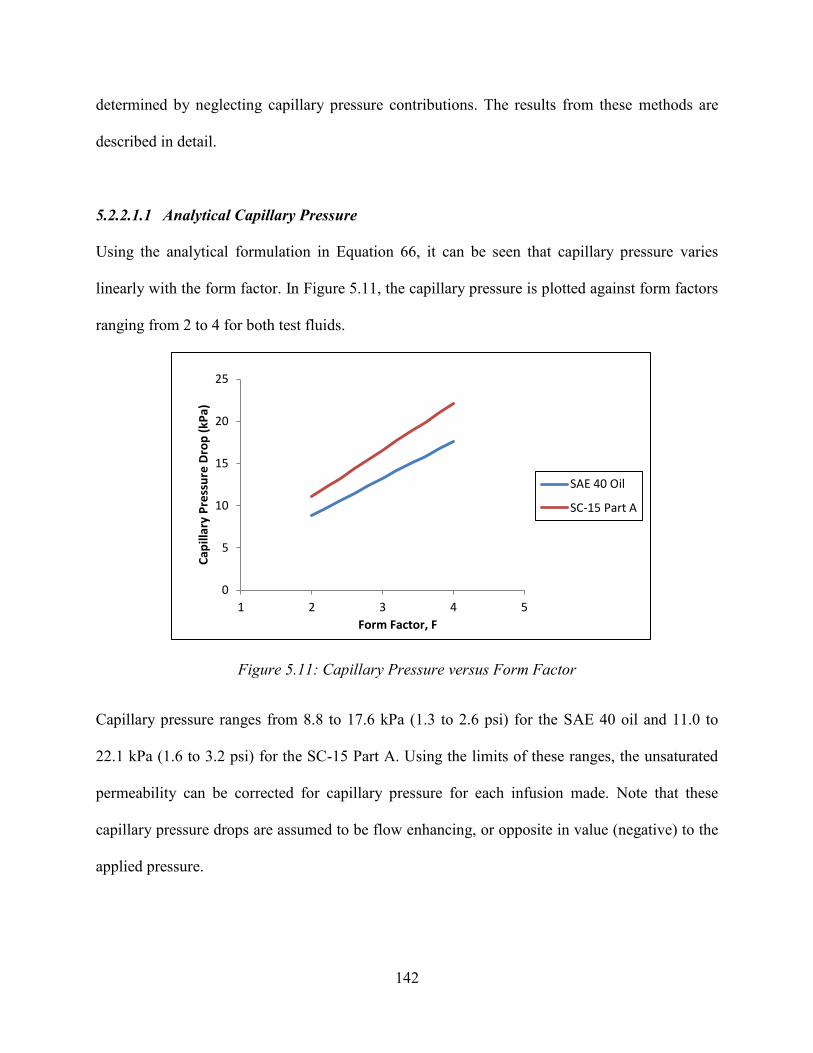
142
determined by neglecting capillary pressure contributions. The results from these methods are
described in detail.
5.2.2.1.1 Analytical Capillary Pressure
Using the analytical formulation in Equation 66, it can be seen that capillary pressure varies
linearly with the form factor. In Figure 5.11, the capillary pressure is plotted against form factors
ranging from 2 to 4 for both test fluids.
Figure 5.11: Capillary Pressure versus Form Factor
Capillary pressure ranges from 8.8 to 17.6 kPa (1.3 to 2.6 psi) for the SAE 40 oil and 11.0 to
22.1 kPa (1.6 to 3.2 psi) for the SC-15 Part A. Using the limits of these ranges, the unsaturated
permeability can be corrected for capillary pressure for each infusion made. Note that these
capillary pressure drops are assumed to be flow enhancing, or opposite in value (negative) to the
applied pressure.
0
5
10
15
20
25
1 2 3 4 5
Cap
illar
y P
ress
ure
Dro
p (
kPa)
Form Factor, F
SAE 40 Oil
SC-15 Part A
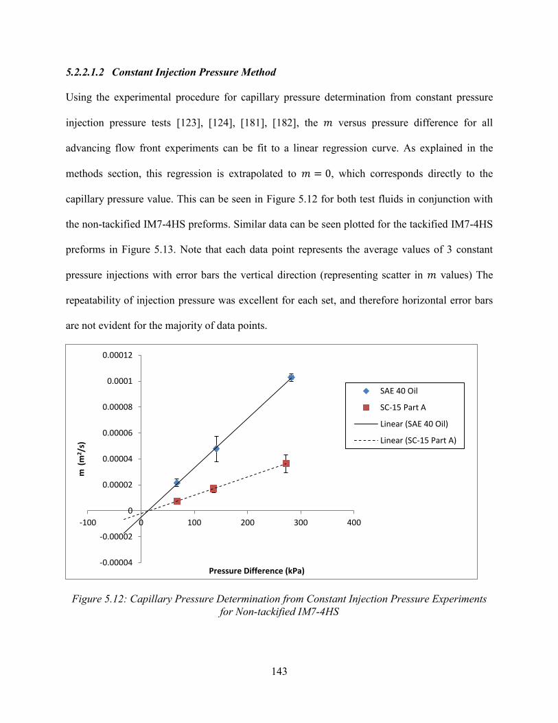
143
5.2.2.1.2 Constant Injection Pressure Method
Using the experimental procedure for capillary pressure determination from constant pressure
injection pressure tests [123], [124], [181], [182], the 𝑚 versus pressure difference for all
advancing flow front experiments can be fit to a linear regression curve. As explained in the
methods section, this regression is extrapolated to 𝑚 = 0, which corresponds directly to the
capillary pressure value. This can be seen in Figure 5.12 for both test fluids in conjunction with
the non-tackified IM7-4HS preforms. Similar data can be seen plotted for the tackified IM7-4HS
preforms in Figure 5.13. Note that each data point represents the average values of 3 constant
pressure injections with error bars the vertical direction (representing scatter in 𝑚 values) The
repeatability of injection pressure was excellent for each set, and therefore horizontal error bars
are not evident for the majority of data points.
Figure 5.12: Capillary Pressure Determination from Constant Injection Pressure Experiments for Non-tackified IM7-4HS
-0.00004
-0.00002
0
0.00002
0.00004
0.00006
0.00008
0.0001
0.00012
-100 0 100 200 300 400
m (m
2/s
)
Pressure Difference (kPa)
SAE 40 Oil
SC-15 Part A
Linear (SAE 40 Oil)
Linear (SC-15 Part A)
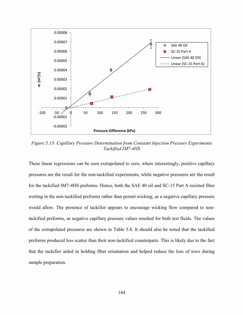
144
Figure 5.13: Capillary Pressure Determination from Constant Injection Pressure Experiments Tackified IM7-4HS
These linear regressions can be seen extrapolated to zero, where interestingly, positive capillary
pressures are the result for the non-tackified experiments, while negative pressures are the result
for the tackified IM7-4HS preforms. Hence, both the SAE 40 oil and SC-15 Part A resisted fiber
wetting in the non-tackified preforms rather than permit wicking, as a negative capillary pressure
would allow. The presence of tackifier appears to encourage wicking flow compared to non-
tackified preforms, as negative capillary pressure values resulted for both test fluids. The values
of the extrapolated pressures are shown in Table 5.8. It should also be noted that the tackified
preforms produced less scatter than their non-tackified counterparts. This is likely due to the fact
that the tackifier aided in holding fiber orientation and helped reduce the loss of tows during
sample preparation.
-0.00002
-0.00001
0
0.00001
0.00002
0.00003
0.00004
0.00005
0.00006
0.00007
0.00008
-100 -50 0 50 100 150 200 250 300
m (m
2/s
)
Pressure Difference (kPa)
SAE 40 Oil
SC-15 Part A
Linear (SAE 40 Oil)
Linear (SC-15 Part A)
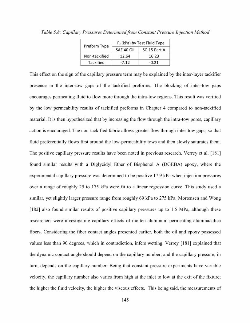
145
Table 5.8: Capillary Pressures Determined from Constant Pressure Injection Method
Preform Type Pc (kPa) by Test Fluid Type
SAE 40 Oil SC-15 Part A
Non-tackified 12.64 16.23
Tackified -7.12 -0.21
This effect on the sign of the capillary pressure term may be explained by the inter-layer tackifier
presence in the inter-tow gaps of the tackified preforms. The blocking of inter-tow gaps
encourages permeating fluid to flow more through the intra-tow regions. This result was verified
by the low permeability results of tackified preforms in Chapter 4 compared to non-tackified
material. It is then hypothesized that by increasing the flow through the intra-tow pores, capillary
action is encouraged. The non-tackified fabric allows greater flow through inter-tow gaps, so that
fluid preferentially flows first around the low-permeability tows and then slowly saturates them.
The positive capillary pressure results have been noted in previous research. Verrey et al. [181]
found similar results with a Diglycidyl Ether of Bisphenol A (DGEBA) epoxy, where the
experimental capillary pressure was determined to be positive 17.9 kPa when injection pressures
over a range of roughly 25 to 175 kPa were fit to a linear regression curve. This study used a
similar, yet slightly larger pressure range from roughly 69 kPa to 275 kPa. Mortensen and Wong
[182] also found similar results of positive capillary pressures up to 1.5 MPa, although these
researchers were investigating capillary effects of molten aluminum permeating alumina/silica
fibers. Considering the fiber contact angles presented earlier, both the oil and epoxy possessed
values less than 90 degrees, which in contradiction, infers wetting. Verrey [181] explained that
the dynamic contact angle should depend on the capillary number, and the capillary pressure, in
turn, depends on the capillary number. Being that constant pressure experiments have variable
velocity, the capillary number also varies from high at the inlet to low at the exit of the fixture;
the higher the fluid velocity, the higher the viscous effects. This being said, the measurements of
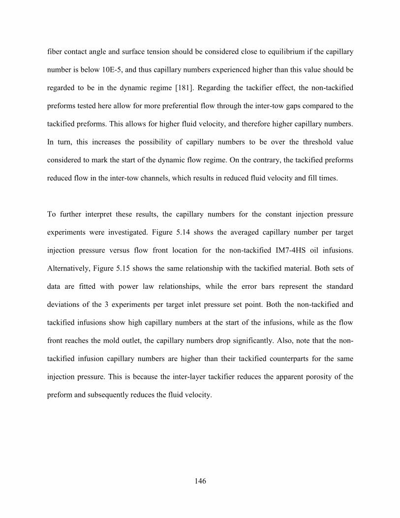
146
fiber contact angle and surface tension should be considered close to equilibrium if the capillary
number is below 10E-5, and thus capillary numbers experienced higher than this value should be
regarded to be in the dynamic regime [181]. Regarding the tackifier effect, the non-tackified
preforms tested here allow for more preferential flow through the inter-tow gaps compared to the
tackified preforms. This allows for higher fluid velocity, and therefore higher capillary numbers.
In turn, this increases the possibility of capillary numbers to be over the threshold value
considered to mark the start of the dynamic flow regime. On the contrary, the tackified preforms
reduced flow in the inter-tow channels, which results in reduced fluid velocity and fill times.
To further interpret these results, the capillary numbers for the constant injection pressure
experiments were investigated. Figure 5.14 shows the averaged capillary number per target
injection pressure versus flow front location for the non-tackified IM7-4HS oil infusions.
Alternatively, Figure 5.15 shows the same relationship with the tackified material. Both sets of
data are fitted with power law relationships, while the error bars represent the standard
deviations of the 3 experiments per target inlet pressure set point. Both the non-tackified and
tackified infusions show high capillary numbers at the start of the infusions, while as the flow
front reaches the mold outlet, the capillary numbers drop significantly. Also, note that the non-
tackified infusion capillary numbers are higher than their tackified counterparts for the same
injection pressure. This is because the inter-layer tackifier reduces the apparent porosity of the
preform and subsequently reduces the fluid velocity.
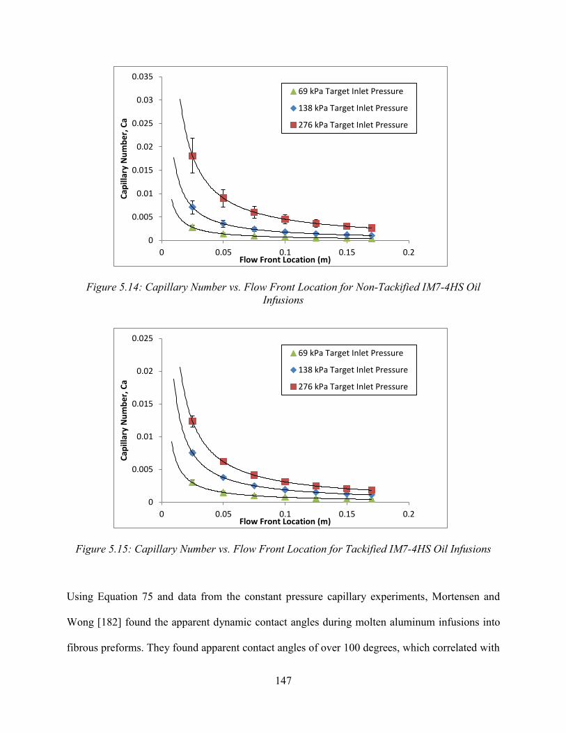
147
Figure 5.14: Capillary Number vs. Flow Front Location for Non-Tackified IM7-4HS Oil Infusions
Figure 5.15: Capillary Number vs. Flow Front Location for Tackified IM7-4HS Oil Infusions
Using Equation 75 and data from the constant pressure capillary experiments, Mortensen and
Wong [182] found the apparent dynamic contact angles during molten aluminum infusions into
fibrous preforms. They found apparent contact angles of over 100 degrees, which correlated with
0
0.005
0.01
0.015
0.02
0.025
0.03
0.035
0 0.05 0.1 0.15 0.2
Cap
illar
y N
um
be
r, C
a
Flow Front Location (m)
69 kPa Target Inlet Pressure
138 kPa Target Inlet Pressure
276 kPa Target Inlet Pressure
0
0.005
0.01
0.015
0.02
0.025
0 0.05 0.1 0.15 0.2
Cap
illar
y N
um
be
r, C
a
Flow Front Location (m)
69 kPa Target Inlet Pressure
138 kPa Target Inlet Pressure
276 kPa Target Inlet Pressure
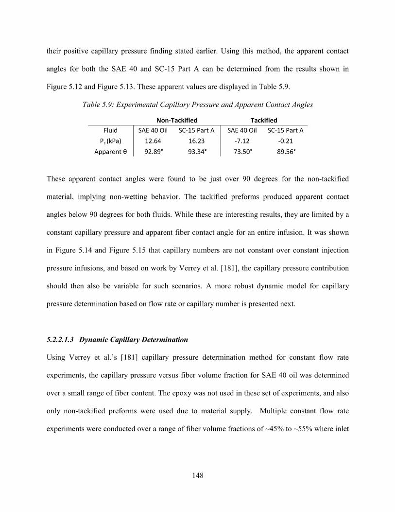
148
their positive capillary pressure finding stated earlier. Using this method, the apparent contact
angles for both the SAE 40 and SC-15 Part A can be determined from the results shown in
Figure 5.12 and Figure 5.13. These apparent values are displayed in Table 5.9.
Table 5.9: Experimental Capillary Pressure and Apparent Contact Angles
Non-Tackified Tackified
Fluid SAE 40 Oil SC-15 Part A SAE 40 Oil SC-15 Part A
Pc (kPa) 12.64 16.23 -7.12 -0.21
Apparent θ 92.89° 93.34° 73.50° 89.56°
These apparent contact angles were found to be just over 90 degrees for the non-tackified
material, implying non-wetting behavior. The tackified preforms produced apparent contact
angles below 90 degrees for both fluids. While these are interesting results, they are limited by a
constant capillary pressure and apparent fiber contact angle for an entire infusion. It was shown
in Figure 5.14 and Figure 5.15 that capillary numbers are not constant over constant injection
pressure infusions, and based on work by Verrey et al. [181], the capillary pressure contribution
should then also be variable for such scenarios. A more robust dynamic model for capillary
pressure determination based on flow rate or capillary number is presented next.
5.2.2.1.3 Dynamic Capillary Determination
Using Verrey et al.’s [181] capillary pressure determination method for constant flow rate
experiments, the capillary pressure versus fiber volume fraction for SAE 40 oil was determined
over a small range of fiber content. The epoxy was not used in these set of experiments, and also
only non-tackified preforms were used due to material supply. Multiple constant flow rate
experiments were conducted over a range of fiber volume fractions of ~45% to ~55% where inlet
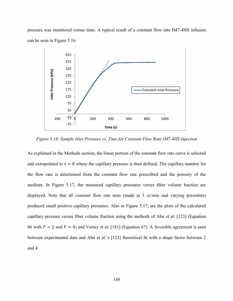
149
pressure was monitored versus time. A typical result of a constant flow rate IM7-4HS infusion
can be seen in Figure 5.16.
Figure 5.16: Sample Inlet Pressure vs. Time for Constant Flow Rate IM7-4HS Injection
As explained in the Methods section, the linear portion of the constant flow rate curve is selected
and extrapolated to 𝑡 = 0 where the capillary pressure is then defined. The capillary number for
the flow rate is determined from the constant flow rate prescribed and the porosity of the
medium. In Figure 5.17, the measured capillary pressures verses fiber volume fraction are
displayed. Note that all constant flow rate tests (made at 3 cc/min and varying porosities)
produced small positive capillary pressures. Also in Figure 5.17, are the plots of the calculated
capillary pressure versus fiber volume fraction using the methods of Ahn et al. [123] (Equation
66 with 𝐹 = 2 and 𝐹 = 4) and Verrey et al. [181] (Equation 67). A favorable agreement is seen
between experimental data and Ahn et al.’s [123] theoretical fit with a shape factor between 2
and 4.
-75
-25
25
75
125
175
225
275
325
375
425
-200 0 200 400 600 800 1000
Inle
t P
ress
ure
(kP
a)
Time (s)
Transient Inlet Pressure
150
Figure 5.17: Experimental and Theoretical (Assumed Positive) Capillary Pressures by Fiber Volume Fraction
Using the constant flow rate experiments to determine the constant 𝑐𝑇 in the Hoffman-Voinov-
Tanner law, the theoretical SAE 40 oil dynamic contact angle versus capillary number can be
plotted for the non-tackified IM7-4HS fabric. This is shown in Figure 5.18.
Figure 5.18: Dynamic Contact Angle vs. Capillary Number using Hoffman-Voinov-Tanner's Law
0
10
20
30
40
50
60
70
80
90
100
0.3 0.4 0.5 0.6 0.7 0.8
Cap
illar
y P
ress
ure
(kP
a)
Fiber Volume Fraction, Vf
Experimental Data
Verrey
Ahn F=4
Ahn F=2
0
30
60
90
120
150
180
0 0.0025 0.005 0.0075 0.01 0.0125 0.015
Dyn
amic
Co
nta
ct A
ngl
e (
de
gre
es)
Capillary Number, Ca
Hoffman-Voinov-Tanner Law
151
A critical capillary number of 0.0022 is found from this plot. Beneath this value, the SAE 40 oil
contact angle is less than 90 degrees and capillary effects are seen to enhance flow, while above
this value, the flow becomes forced and the oil behaves as a non-wetting fluid. Verrey et al.
[181] saw similar results with their epoxy, as they found a critical capillary number of 0.014,
where the epoxy changed from wetting to non-wetting. The critical value of 0.0022 found from
the constant flow rate experiments, although small, compares well with the constant-pressure-
produced capillary pressure data, in which low capillary numbers (seen in Figure 5.14), were
found to a produce positive capillary pressures. The capillary numbers for all SAE 40 constant
pressure infusions were averaged over the flow distance to produce a value of 0.005. Using this
average capillary number and the constant flow rate data, the experimental capillary pressure
drop versus capillary number can be displayed and compared to the theoretical values. This
comparison is made in Figure 5.19.
Figure 5.19: Theoretical and Experimental Capillary Pressures vs. Capillary Number for IM7-4HS with SAE 40 Oil
-20
-15
-10
-5
0
5
10
15
20
25
30
0 0.002 0.004 0.006 0.008 0.01
Cap
illar
y P
resu
re (
kPa)
Capillary Number, Ca
Theoretical - Hoffman-Voinov-Tanner Law
Experimental - Constant Flow Rate Injections
Experimental - Constant Pressure Injections
152
The experimental data produces a favorable fit with the theoretical formulation. It can also be
seen here that capillary numbers lower than the critical 0.0022 value produce negative capillary
pressures, while the numbers higher than the threshold produce positive values. Hence, flow is
enhanced beneath the critical capillary number and resisted above it. This will then inevitably
alter the preform permeability, and permeability could be expressed a function of capillary
number (which is a function of fluid velocity). The magnitude of capillary the effect then comes
into consideration, as the experimentally determined capillary pressures are generally seen to be
small compared to normal LCM injection pressures. The significance of this capillary effect in
terms of preform permeability is explored next.
5.2.2.2 Permeability Correction for Capillary Effects
This study compares four different methods for correcting permeability for capillary pressure.
These methods include: 1) a dynamic correction described earlier using the Hoffman-Voinov-
Tanner law paired with constant flow rate experiments, 2) a constant capillary pressure
correction derived from constant pressure injection experiments, 3) a theoretical capillary
pressure correction described by Ahn et al. [123], and 4) neglecting capillary effects altogether
(i.e. no correction). The dynamic correction method from the Hoffman-Voinov-Tanner law was
only produced for the SAE 40 oil infusions with non-tackified preforms, and is not used for the
SC-15 Part A tests. A comparison of the four correction methods and capillary values is shown
in Table 5.10 for the SAE 40 oil experiments for both tackified and non-tackified preforms.
153
Table 5.10: Capillary Pressure Correction Method Comparison for SAE 40 Oil and IM7-4HS
Method Hoffman-Voinov-Tanner
Constant Pressure Injections
Experiments
Ahn's Theoretical
Formulation, F=4
Ahn's Theoretical
Formulation, F=2
Neglecting Capillary Effects
Correction Value Type
Dynamic Constant Constant Constant Constant
Pc (kPa) for Non-tackified Preforms
Function of Ca
12.64 -17.64 -8.82 0
Pc (kPa) for
Tackified Preforms
N/A -7.12 -17.64 -8.82 0
Due to the variable capillary number in the constant pressure infusions, the Hoffman-Voinov-
Tanner method gives a dynamic range of capillary pressures during the infusion. This is difficult
to consider without employing numerical models in terms of permeability correction. In this
study, the capillary number over the entire infusion length was averaged so a simple correction
could be applied based on the injection pressure. The average capillary numbers and resulting
capillary pressures from the Hoffman-Voinov-Tanner fit can be seen in Table 5.11 for all nine
SAE 40 oil infusions with the non-tackified preforms.

154
Table 5.11: Average Capillary Numbers and Pressure from the Hoffman-Voinov-Tanner Correction for non-tackified IM7-4HS and SAE 40 Oil
Target Injection Pressure
(kPa)
Run #
Actual Injection Pressure
(kPa)
Average Ca Over
Length (-)
Pc from Hoffman-
Voinov-Tanner Fit (kPa)
69
1 67.2 0.00134 -5.0
2 66.9 0.00142 -4.6
3 68.0 0.00173 -2.6
138
1 141.1 0.00295 3.6
2 141.3 0.00406 7.9
3 141.3 0.00436 8.9
276
1 280.0 0.00869 18.6
2 284.9 0.00835 18.1
3 278.2 0.01196 22.3
For the 69 kPa (10 psi) injection pressure range, the resulting capillary pressures were negative,
while at the 138 and 276 kPa (20 and 40 psi) ranges the capillary pressures were positive and
increasing in magnitude, respectively. Figure 5.20 shows a comparison of the capillary
correction methods and their effect on the unsaturated permeability of non-tackified IM7-4HS
with SAE 40 oil.
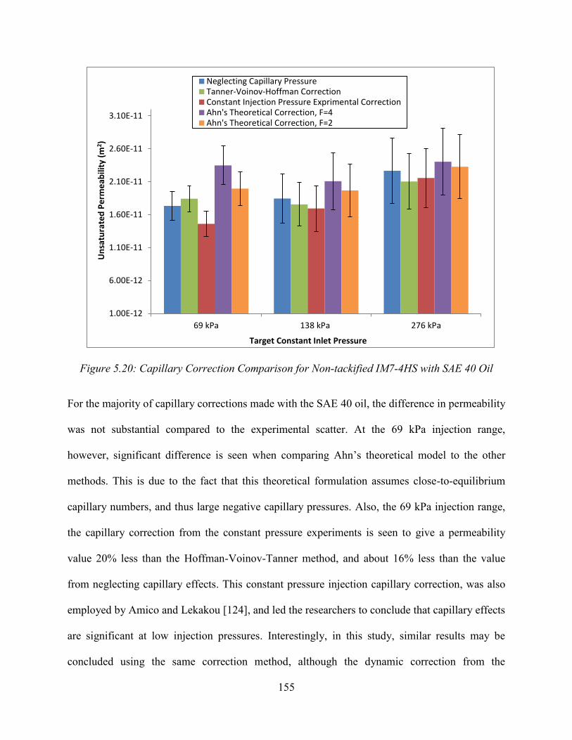
155
Figure 5.20: Capillary Correction Comparison for Non-tackified IM7-4HS with SAE 40 Oil
For the majority of capillary corrections made with the SAE 40 oil, the difference in permeability
was not substantial compared to the experimental scatter. At the 69 kPa injection range,
however, significant difference is seen when comparing Ahn’s theoretical model to the other
methods. This is due to the fact that this theoretical formulation assumes close-to-equilibrium
capillary numbers, and thus large negative capillary pressures. Also, the 69 kPa injection range,
the capillary correction from the constant pressure experiments is seen to give a permeability
value 20% less than the Hoffman-Voinov-Tanner method, and about 16% less than the value
from neglecting capillary effects. This constant pressure injection capillary correction, was also
employed by Amico and Lekakou [124], and led the researchers to conclude that capillary effects
are significant at low injection pressures. Interestingly, in this study, similar results may be
concluded using the same correction method, although the dynamic correction from the
1.00E-12
6.00E-12
1.10E-11
1.60E-11
2.10E-11
2.60E-11
3.10E-11
69 kPa 138 kPa 276 kPa
Un
satu
rate
d P
erm
eab
ility
(m
2 )
Target Constant Inlet Pressure
Neglecting Capillary PressureTanner-Voinov-Hoffman CorrectionConstant Injection Pressure Exprimental CorrectionAhn's Theoretical Correction, F=4Ahn's Theoretical Correction, F=2

156
Hoffman-Voinov-Tanner method showed no significant difference from neglecting capillary
effects at all injection pressures. It is assumed here that the Hoffman-Voinov-Tanner correction
is more accurate than the constant pressure injection value as it accounts more robustly for
changes in capillary number. Thus, this constant pressure method to determine capillary pressure
may lead to inaccurate conclusions in terms of permeability correction. Verrey et al. [181] also
noted that the constant pressure method should not be used to correct for capillary effects as the
velocity in these experiments changes strongly throughout testing. Regardless of sign on the
capillary pressure term, these effects are seen to become negligible as injection pressure
increases. This is because the capillary pressure drop accounts for less of the total pressure drop
used to determine permeability as injection pressure increases. The permeability comparison
with capillary correction methods for the tackified IM7-4HS tested with SAE 40 oil is shown in
Figure 5.21.
Figure 5.21: Capillary Correction Comparison for Tackified IM7-4HS with SAE 40 Oil
1.00E-12
6.00E-12
1.10E-11
1.60E-11
2.10E-11
69 kPa 138 kPa 276 kPa
Un
satu
rate
d P
erm
eab
ility
(m
2)
Target Constant Inlet Pressure
Neglecting Capillary PressureConstant Injection Pressure Experimental CorrectionAhn's Theoretical Correction, F=4Ahn's Theoretical Correction, F=2
157
Note that the Hoffman-Voinov-Tanner dynamic correction model was not produced for the
tackified samples. Compared to the non-tackified data, the tackified unsaturated permeability
measurements produced less experimental scatter. This is because the presence of tackifier holds
fiber and tow orientation stable throughout sample preparation, while the non-tackified preforms
were more likely to be subject to tow loss and preform deformation. At the 69 kPa target
injection pressure range, the permeability was much more sensitive to the correction method than
at the higher injection pressures. This again points to the importance of capillary pressure at low
injection pressures, while the higher pressures showed no statistical difference in permeability
was observed.
Overall from the IM7-4HS testing with the oil, it can be concluded that the capillary correction
method from the Hoffman-Voinov-Tanner law described in this study is the most robust method
presented. While being hypothesized as the most accurate, this method still did not show any
significant difference from neglecting capillary effects altogether in the unsaturated permeability
calculation at any injection pressure tested. A comparison of the capillary correction methods
and their values for the SC-15 infusions in preforms with and without tackifier are shown in
Table 5.12.

158
Table 5.12: Capillary Pressure Correction Method Comparison for SC-15 Part A and IM7-4HS
Method Hoffman-
Voinov-Tanner
Constant Pressure Injections
Experiments
Ahn's Theoretical
Formulation, F=4
Ahn's Theoretical
Formulation, F=2
Neglecting Capillary Effects
Correction Value Type
Dynamic Constant Constant Constant Constant
Pc (kPa) for Non-tackified Preforms
N/A 16.23 22.13 11.06 0
Pc (kPa) for
Tackified Preforms
N/A -0.21 22.13 11.06 0
Again, note that the Hoffman-Voinov-Tanner correction for capillary pressure is not shown here,
as it was not determined for the SC-15. In Figure 5.22, the capillary correction permeability
comparison for the non-tackified IM7-4HS tests with SC-15 Part A is shown.
Figure 5.22: Capillary Correction Comparison for Non-tackified IM7-4HS with SC-15 Part A
1.00E-12
6.00E-12
1.10E-11
1.60E-11
2.10E-11
2.60E-11
3.10E-11
69 kPa 138 kPa 276 kPa
Un
satu
rate
d P
erm
eab
ility
(m
2)
Target Constant Inlet Pressure
Neglecting Capillary Pressure
Constant Injection Pressure Exprimental Correction
Ahn's Theoretical Correction, F=4
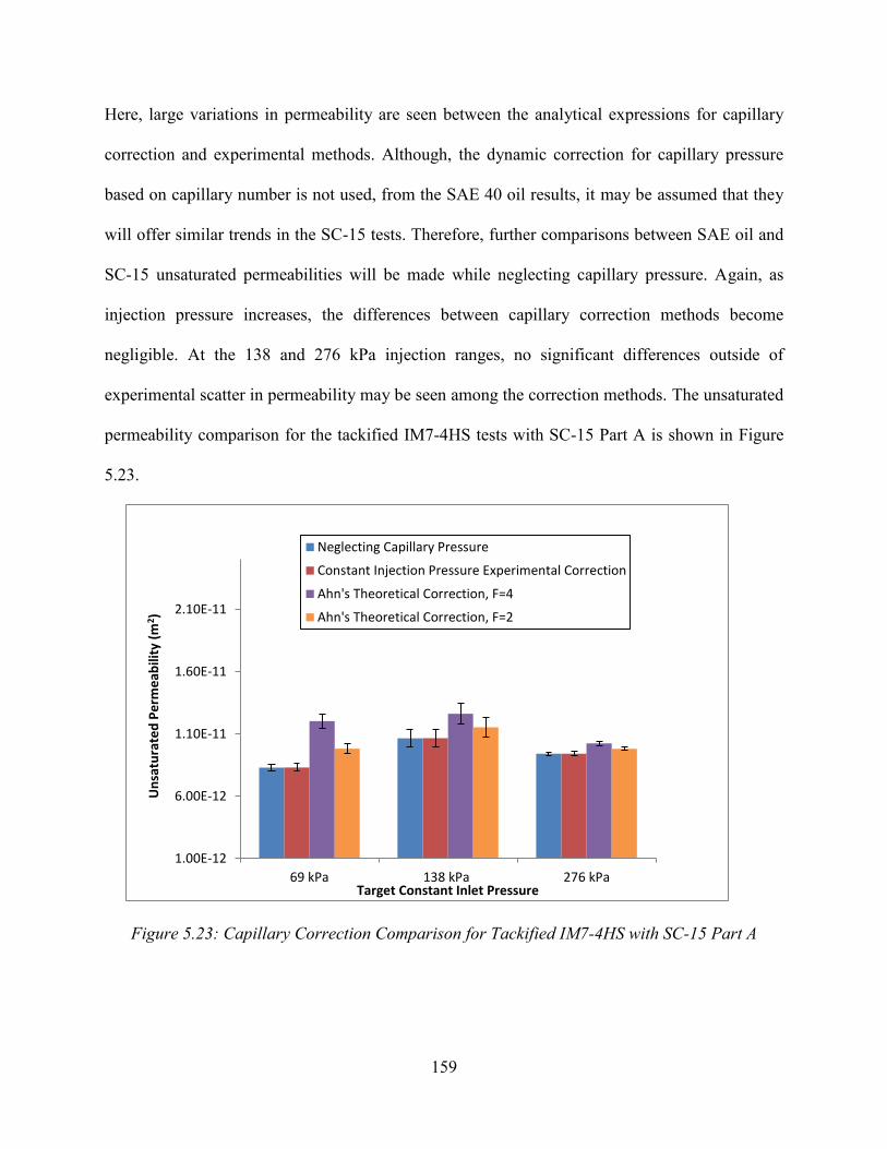
159
Here, large variations in permeability are seen between the analytical expressions for capillary
correction and experimental methods. Although, the dynamic correction for capillary pressure
based on capillary number is not used, from the SAE 40 oil results, it may be assumed that they
will offer similar trends in the SC-15 tests. Therefore, further comparisons between SAE oil and
SC-15 unsaturated permeabilities will be made while neglecting capillary pressure. Again, as
injection pressure increases, the differences between capillary correction methods become
negligible. At the 138 and 276 kPa injection ranges, no significant differences outside of
experimental scatter in permeability may be seen among the correction methods. The unsaturated
permeability comparison for the tackified IM7-4HS tests with SC-15 Part A is shown in Figure
5.23.
Figure 5.23: Capillary Correction Comparison for Tackified IM7-4HS with SC-15 Part A
1.00E-12
6.00E-12
1.10E-11
1.60E-11
2.10E-11
69 kPa 138 kPa 276 kPa
Un
satu
rate
d P
erm
eab
ility
(m
2)
Target Constant Inlet Pressure
Neglecting Capillary Pressure
Constant Injection Pressure Experimental Correction
Ahn's Theoretical Correction, F=4
Ahn's Theoretical Correction, F=2
160
Large variations in the permeability correction again are seen at the lowest injection pressure. As
the injection pressure increases, the difference between correction methods is seen to diminish
drastically. The tackifier again shows aid in reducing test-to-test scatter.
For both test fluids employed, it can be concluded that large variations between permeability are
seen only at the lowest injection pressure range (69 kPa) depending on the capillary correction
method chosen. It can then be concluded that capillary pressures may only be significant for
these IM7-4HS preforms when injections are made at 69 kPa or less. The permeability
determined using the dynamic method for capillary correction has been shown to be very close to
the permeability determined by neglecting capillary pressure. Also, depending on the injection
pressure used, infiltrating flow may result in forced or wicking flow as capillary pressure is a
function of capillary number.
5.2.2.3 Fluid Type Effects
A comparison of unsaturated permeability with fluid type is shown in Figure 5.24 for the non-
tackified. Capillary pressure effects are neglected in this comparison. The data from Figure 5.24
are tabulated following in Table 5.13.

161
Figure 5.24: Unsaturated Permeability of Non-tackified IM7-4HS by Test Fluid
Table 5.13: Non-tackified IM7-4HS Unsaturated Permeability by Target Constant Inlet Pressure
Sxx Permeability by Test Fluid and Target Inlet Pressure (m2)
Run # 69 kPa 138 kPa 276 kPa
SAE 40 Oil
SC-15 Part A SAE 40
Oil SC-15 Part A
SAE 40 Oil
SC-15 Part A
Run 1 1.56E-11 1.31E-11 1.42E-11 1.39E-11 2.04E-11 1.39E-11
Run 2 1.66E-11 1.48E-11 2.00E-11 1.86E-11 1.93E-11 2.08E-11
Run 3 1.98E-11 1.43E-11 2.12E-11 1.70E-11 2.83E-11 1.79E-11
Avg. 1.73E-11 1.41E-11 1.85E-11 1.65E-11 2.27E-11 1.76E-11
StDev 2.22E-12 8.95E-13 3.77E-12 2.37E-12 4.92E-12 3.47E-12
CV (%)
12.8 6.4 20.4 14.3 21.7 19.8
The fluid type comparison for the tackified IM7-4HS unsaturated permeability measurements is
shown in Figure 5.25, and following in Table 5.14 are the numerical data of this plot.
1.00E-12
6.00E-12
1.10E-11
1.60E-11
2.10E-11
2.60E-11
3.10E-11
69 kPa 138 kPa 276 kPa
Un
satu
rate
d P
erm
eab
ility
(m
2 )
Target Constant Injection Pressure
NAPA SAE 40 Oil
SC-15 Part A
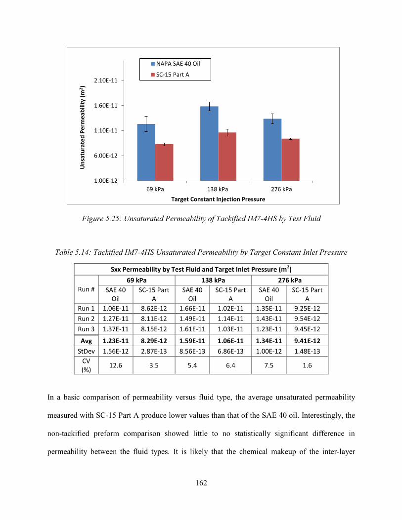
162
Figure 5.25: Unsaturated Permeability of Tackified IM7-4HS by Test Fluid
Table 5.14: Tackified IM7-4HS Unsaturated Permeability by Target Constant Inlet Pressure
Sxx Permeability by Test Fluid and Target Inlet Pressure (m2)
Run # 69 kPa 138 kPa 276 kPa
SAE 40 Oil
SC-15 Part A
SAE 40 Oil
SC-15 Part A
SAE 40 Oil
SC-15 Part A
Run 1 1.06E-11 8.62E-12 1.66E-11 1.02E-11 1.35E-11 9.25E-12
Run 2 1.27E-11 8.11E-12 1.49E-11 1.14E-11 1.43E-11 9.54E-12
Run 3 1.37E-11 8.15E-12 1.61E-11 1.03E-11 1.23E-11 9.45E-12
Avg 1.23E-11 8.29E-12 1.59E-11 1.06E-11 1.34E-11 9.41E-12
StDev 1.56E-12 2.87E-13 8.56E-13 6.86E-13 1.00E-12 1.48E-13
CV (%)
12.6 3.5 5.4 6.4 7.5 1.6
In a basic comparison of permeability versus fluid type, the average unsaturated permeability
measured with SC-15 Part A produce lower values than that of the SAE 40 oil. Interestingly, the
non-tackified preform comparison showed little to no statistically significant difference in
permeability between the fluid types. It is likely that the chemical makeup of the inter-layer
1.00E-12
6.00E-12
1.10E-11
1.60E-11
2.10E-11
69 kPa 138 kPa 276 kPa
Un
satu
rate
d P
erm
eab
ility
(m
2)
Target Constant Injection Pressure
NAPA SAE 40 Oil
SC-15 Part A

163
tackifier alters the wettability between the resin and the IM7 fibers. It may also be possible that
the tackifier causes more intra-tow flow and therefore the influence of capillary effects are
magnified compared to the non-tackified samples. Capillary effects have been noted by
researchers to produce significant difference in permeability among fluid types [117]. Other
reasoning could be that with the addition of tackifier, the test-by-test variation significantly
reduced, so that less change in permeability is needed to produce statistically significant
differences. This allows the possibilities of other test inconsistencies (e.g. user variations, small
ambient temperature changes, etc.) to have larger influence on test outcome.
Researchers including Hammond et al. [43], [133] and Luo et al. [116] have concluded that
different test fluids had little effect on measured permeability. Although, it should be noted that
Hammond’s [43], [133] studies directly compared measurements of saturated permeability with
different fluids and did not directly compare unsaturated measurements of varying fluids. This is
important to note as saturated permeability experiments involve single phase flow, while
unsaturated scenarios inherently involve a multi-phase flow. From these current results it can be
concluded that unsaturated non-tackified IM7-4HS permeability does not depend on test fluid
when the injection pressure is high enough for capillary effects to be neglected, while tackified
IM7-4HS permeability is sensitive to the test fluid employed. With this in consideration, future
preform permeability characterization should be conducted with the resin that will be employed
during actual manufacturing. Also, at low injection pressure or flow rates, capillary effects may
cause significant differences in permeability depending on the test fluid. At the high
pressures/flow rates (often seen in RTM processing), viscous forces dominate and permeability
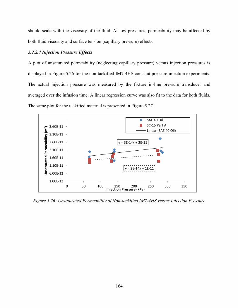
164
should scale with the viscosity of the fluid. At low pressures, permeability may be affected by
both fluid viscosity and surface tension (capillary pressure) effects.
5.2.2.4 Injection Pressure Effects
A plot of unsaturated permeability (neglecting capillary pressure) versus injection pressures is
displayed in Figure 5.26 for the non-tackified IM7-4HS constant pressure injection experiments.
The actual injection pressure was measured by the fixture in-line pressure transducer and
averaged over the infusion time. A linear regression curve was also fit to the data for both fluids.
The same plot for the tackified material is presented in Figure 5.27.
Figure 5.26: Unsaturated Permeability of Non-tackified IM7-4HS versus Injection Pressure
y = 3E-14x + 2E-11
y = 2E-14x + 1E-11
1.00E-12
6.00E-12
1.10E-11
1.60E-11
2.10E-11
2.60E-11
3.10E-11
3.60E-11
0 50 100 150 200 250 300 350
Un
satu
rate
d P
erm
eab
ility
(m
2)
Injection Pressure (kPa)
SAE 40 Oil
SC-15 Part A
Linear (SAE 40 Oil)
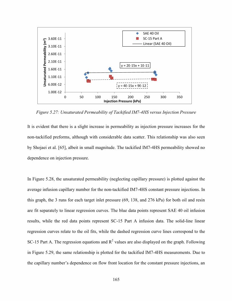
165
Figure 5.27: Unsaturated Permeability of Tackified IM7-4HS versus Injection Pressure
It is evident that there is a slight increase in permeability as injection pressure increases for the
non-tackified preforms, although with considerable data scatter. This relationship was also seen
by Shojaei et al. [65], albeit in small magnitude. The tackified IM7-4HS permeability showed no
dependence on injection pressure.
In Figure 5.28, the unsaturated permeability (neglecting capillary pressure) is plotted against the
average infusion capillary number for the non-tackified IM7-4HS constant pressure injections. In
this graph, the 3 runs for each target inlet pressure (69, 138, and 276 kPa) for both oil and resin
are fit separately to linear regression curves. The blue data points represent SAE 40 oil infusion
results, while the red data points represent SC-15 Part A infusion data. The solid-line linear
regression curves relate to the oil fits, while the dashed regression curve lines correspond to the
SC-15 Part A. The regression equations and R2 values are also displayed on the graph. Following
in Figure 5.29, the same relationship is plotted for the tackified IM7-4HS measurements. Due to
the capillary number’s dependence on flow front location for the constant pressure injections, an
y = 2E-15x + 1E-11
y = 4E-15x + 9E-12
1.00E-12
6.00E-12
1.10E-11
1.60E-11
2.10E-11
2.60E-11
3.10E-11
3.60E-11
0 50 100 150 200 250 300 350
Un
satu
rate
d P
erm
eab
ility
(m
2)
Injection Pressure (kPa)
SAE 40 Oil
SC-15 Part A
Linear (SAE 40 Oil)

166
average capillary number was determined over the preform length before being plotted against
the corresponding permeability.
Figure 5.28: Unsaturated Permeability of Non-tackified IM7-4HS versus Capillary Number
Figure 5.29: Unsaturated Permeability of Tackified IM7-4HS versus Capillary Number
y = 1E-08x + 1E-12 R² = 0.9985
y = 5E-09x - 7E-13 R² = 0.9981
y = 2E-09x - 1E-12 R² = 0.999
y = 1E-08x + 2E-12 R² = 0.9651
y = 5E-09x + 3E-12 R² = 0.9986
y = 3E-09x - 6E-13 R² = 0.9991
1.00E-12
6.00E-12
1.10E-11
1.60E-11
2.10E-11
2.60E-11
3.10E-11
0 0.002 0.004 0.006 0.008 0.01 0.012 0.014
Un
satu
rate
d P
erm
eab
ility
(m
2 )
Capillary Number, Ca
SAE 40 Oil - 69 kPa Target Pressure138 kPa Target Pressure276 kPa Target PressureSC-15 Part A - 69 kPa Target Pressure138 kPa Target Pressure276 kPa Target Pressure
y = 6E-09x + 3E-12 R² = 0.8538
y = 6E-09x - 5E-12 R² = 0.953
y = 2E-09x - 1E-12 R² = 0.9984
y = 5E-09x + 4E-12 R² = 0.2183
y = 6E-09x - 3E-12 R² = 0.9938
y = 2E-09x + 2E-12 R² = 0.2117
1.00E-12
6.00E-12
1.10E-11
1.60E-11
2.10E-11
2.60E-11
3.10E-11
0 0.002 0.004 0.006 0.008 0.01
Un
satu
rate
d P
erm
eab
ility
(m
2)
Capillary Number, Ca
SAE 40 Oil - 69 kPa Target Pressure
138 kPa Target Pressure
276 kPa Target Pressure
SC-15 Part A - 69 kPa Target Pressure
138 kPa Target Pressure
276 kPa Target Pressure
167
Within each injection pressure range, the permeability increases with capillary number for both
fluids in preforms with and without tackifier. The majority of these linear regression curves show
a high value of fit. Also, the oil and resin regression curves for each corresponding target
injection pressure range are similar in slope, which alludes to the fact that this behavior is likely
characteristic to the fabric architecture, not the fluid. Interestingly, no clear trend in permeability
versus capillary number can be seen across all injection pressure ranges, which corroborates with
the findings of Figure 5.26 and Figure 5.27. Hammond et al. [43], [133] found permeability to be
independent of capillary number, while Young et al. [142] saw large increases in permeability
with fluid velocity for random fiber and bidirectional fiber mats. Although the velocities used
were high at 1 to 11 cm/s. In a study by Shojaei et al. [65], a critical velocity of only 0.2 cm/s
was calculated for the glass fabric used. Velocities over this were hypothesized to produce
permeability values that increased with increasing flow rate, which is induced by increasing
pressure. Being that within each injection pressure range, an increase in permeability over
capillary number was seen, it is possible that this may be due to the fluid passing a critical
velocity barrier similar to that reported by Shojaei et al. [65].
5.2.2.5 Tackifier Effects
A comparison of unsaturated IM7-4HS permeability measurements with and without the inter-
layer tackifier is shown in Figure 5.30. This is shown with both test fluids, while capillary
pressure is neglected in the permeability formulations.
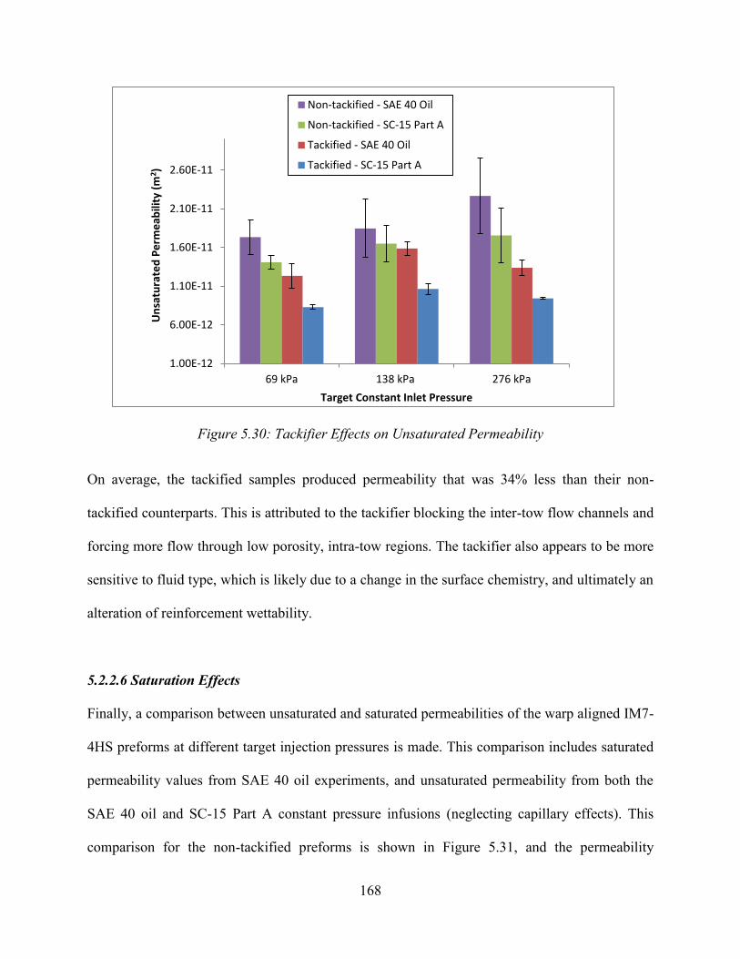
168
Figure 5.30: Tackifier Effects on Unsaturated Permeability
On average, the tackified samples produced permeability that was 34% less than their non-
tackified counterparts. This is attributed to the tackifier blocking the inter-tow flow channels and
forcing more flow through low porosity, intra-tow regions. The tackifier also appears to be more
sensitive to fluid type, which is likely due to a change in the surface chemistry, and ultimately an
alteration of reinforcement wettability.
5.2.2.6 Saturation Effects
Finally, a comparison between unsaturated and saturated permeabilities of the warp aligned IM7-
4HS preforms at different target injection pressures is made. This comparison includes saturated
permeability values from SAE 40 oil experiments, and unsaturated permeability from both the
SAE 40 oil and SC-15 Part A constant pressure infusions (neglecting capillary effects). This
comparison for the non-tackified preforms is shown in Figure 5.31, and the permeability
1.00E-12
6.00E-12
1.10E-11
1.60E-11
2.10E-11
2.60E-11
69 kPa 138 kPa 276 kPa
Un
satu
rate
d P
erm
eab
ility
(m
2 )
Target Constant Inlet Pressure
Non-tackified - SAE 40 Oil
Non-tackified - SC-15 Part A
Tackified - SAE 40 Oil
Tackified - SC-15 Part A

169
comparison for the tackified material is shown in Figure 5.32. The saturated values were
presented in Chapter 4 and were obtained from the power law fit at the 54.6% fiber volume
fraction of the unsaturated experiments.
Figure 5.31: Saturated vs. Unsaturated Sxx Permeability for Warp-Aligned Non-tackified IM7-4HS at 54.6% Vf
Figure 5.32: Saturated vs. Unsaturated Sxx Permeability for Warp-Aligned Tackified IM7-4HS at
54.6% Vf
1E-12
6E-12
1.1E-11
1.6E-11
2.1E-11
2.6E-11
3.1E-11
69 kPa 138 kPa 276 kPa
Un
satu
rate
d P
erm
eab
ility
(m
2 )
Target Constant Inlet Pressure
Saturated Permeability - SAE 40 Oil
Unsaturated Permeability - SAE 40 Oil
Unsaturated Permeability - SC-15 Part A
1E-12
6E-12
1.1E-11
1.6E-11
2.1E-11
0 0 0
Un
satu
rate
d P
erm
eab
ility
(m
2)
Target Constant Inlet Pressure
Saturated Permeability - SAE 40 Oil
Unsaturated Permeability - SAE 40 Oil
Unsaturated Permeability - SC-15 Part A
170
Permeabilities of saturated and unsaturated measurements are well within experimental scatter of
each other for the all the non-tackified measurements. For the tackified material, both the
saturated and unsaturated permeabilities measured using a SAE 40 oil were also well within
experimental scatter of each other for all injection pressure ranges. Interestingly, the unsaturated
permeability of the tackified IM7-4HS measured with SC-15 Part A tested significantly lower
than the saturated and unsaturated cases measured with oil. As discussed earlier, it is likely that
the addition of the tackifier significantly alters the wetting behavior between the oil and resin. It
is then concluded that for the non-tackified IM7-4HS, fluid type does not affect permeability,
while the addition of tackifier creates significant difference in permeability depending on the
fluid type used. Other researchers have found the difference between saturated and unsaturated
permeability to be negligible depending on the preform type [43], [133]. This could be due to the
fact that certain fabric architectures may mitigate the role of the dual scale porosity, which has
been stated to have larger effects when uninterrupted flow channels are present in the
reinforcement [130]. The dual scale porosity is a function of saturation, while capillary effects
can cause differences in flow front evolution [138]. By comparing saturated and advancing front
permeability measurements directly, one is essentially neglecting saturation effects. If this
simplification can be justified, material characterization can become more efficient as saturated
flow tests, which can deliver more data per sample, can be used. For this study, saturated
measurements made in a separate test fixture have produced values within scatter of the
advancing front tests at a single volume fraction (the environment more native to actual LCM
infusions) for the non-tackified IM7-4HS. Extending this relationship to other fiber volume
fractions is not completed in this thesis due to material constraints, but the assumption is
reasonable. On the contrary, the tackified IM7-4HS saturated versus unsaturated permeability
171
results show significant difference. It is hypothesized that the addition of tackifier may
encourage more intra-tow flow and capillary effects due to the inter-tow channel blockages.
Also, the addition of tackifier may result in enough flow channel geometry change to create a
more severe dual-scale porosity compared to the non-tackified architecture, resulting in the
significant unsaturated versus saturated permeability difference.
5.3 Conclusions
Fluid surface tension and IM7 fiber contact angle measurements were performed with SAE 40
motor oil and SC-15 Part A epoxy resin. The epoxy was found to be a better wetting fluid with
the IM7 fiber. Then, constant pressure unsaturated permeability experiments were conducted to
investigate fluid effects on the permeability of IM7-4HS preforms. Capillary pressures were
calculated with theoretical models and experimental measurements and used in calculation of
unsaturated permeability. The theoretical expression for capillary pressure was found to affect
the unsaturated permeability calculations at low injection pressures. The theoretical formulation
was determined to be a poor representation of capillary effects, as it was based on idealized fiber
packing arrangements and close-to-equilibrium fiber contact angle values. A constant injection
pressure experimental technique was used to determine capillary pressure and produced positive
capillary pressures, inferring non-wetting behavior during infusion for the non-tackified
preforms. The tackified preforms, on the contrary, produced negative capillary pressures. It was
hypothesized that the presence of inter-layer tackifier forces more flow through the intra-tow
capillaries, and encourages wicking flow. Further, constant flow rate experiments were run to
determine capillary pressure over a range of capillary numbers. Positive capillary pressures were
also found here for the non-tackified preforms. Starting with the formulation proposed by Verrey

172
et al. [181] and the constant flow rate data, a dynamic capillary correction method was employed
based on average infusion capillary number. The resulting capillary pressures showed little effect
on the unsaturated permeability calculation. Significant differences between the SAE 40 motor
oil and the SC-15 Part A epoxy were only seen at low injection pressures (<69 kPa) for the non-
tackified preforms, while the tackified fabric showed significant differences in permeability
depending on the test fluid. It was concluded that the resin used in manufacturing should be also
be used in preform characterization. Unsaturated permeability data were also compared with
saturated permeability data and the values were within experimental scatter of each other for the
non-tackified fabric. The tackified fabric, however, showed difference between saturated
permeability and unsaturated permeability measured with differing test fluid. This provides that
accurate characterization for LCM mold fill models can be produced from saturated permeability
measurements for the non-tackified four-harness satin fabric, while tackified fabric should be
characterized in unsaturated infusions with the resin that is used in manufacturing.
Although in earlier discussions, specific test parameters and effects are highlighted for their
influence on preform permeability, these effects are closely tied to each other and their
relationships should be noted. Preform permeability is a function of saturation. In saturated flow,
a single phase of fluid propagates through the porous media that is already fully saturated with
the permeant. In advancing front or unsaturated scenarios, the flow will be a multiphase where
the permeating fluid displaces an existing fluid of different properties (e.g. air in most LCM
systems). The difference between saturated and unsaturated flow have been shown
experimentally to be significantly different dependent on the reinforcement type [139]. For
preforms with a dual scale porous nature, the difference in saturated and unsaturated flow is
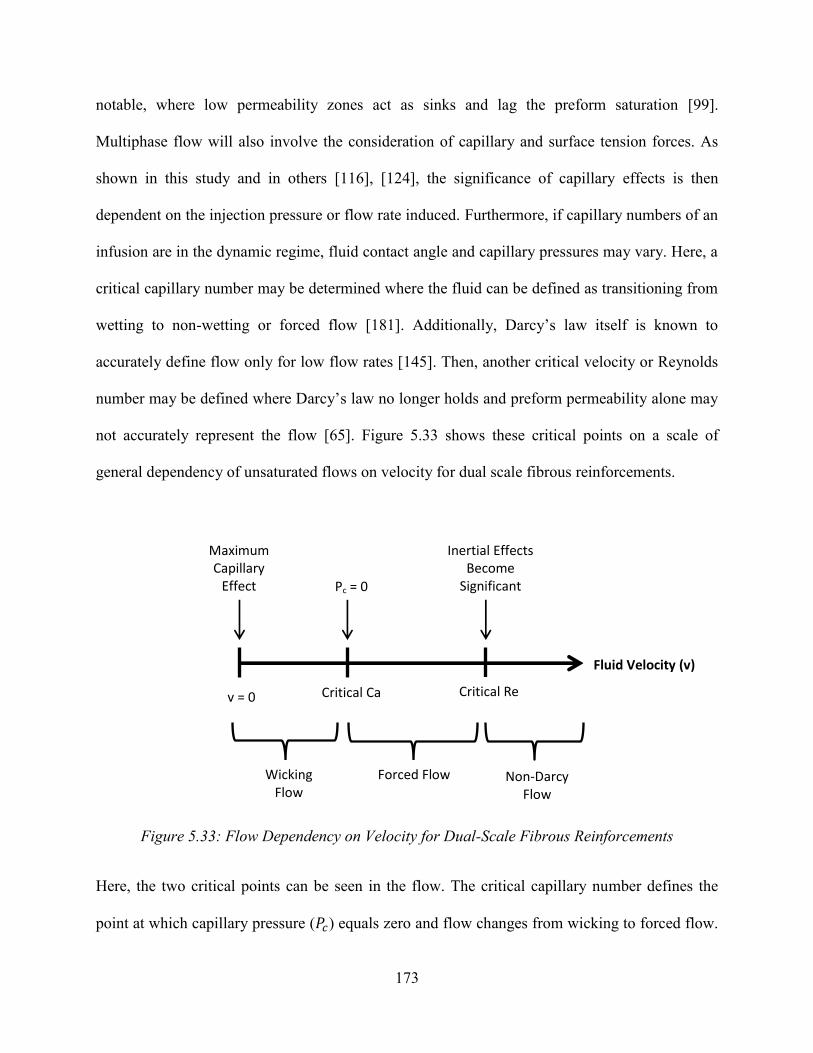
173
notable, where low permeability zones act as sinks and lag the preform saturation [99].
Multiphase flow will also involve the consideration of capillary and surface tension forces. As
shown in this study and in others [116], [124], the significance of capillary effects is then
dependent on the injection pressure or flow rate induced. Furthermore, if capillary numbers of an
infusion are in the dynamic regime, fluid contact angle and capillary pressures may vary. Here, a
critical capillary number may be determined where the fluid can be defined as transitioning from
wetting to non-wetting or forced flow [181]. Additionally, Darcy’s law itself is known to
accurately define flow only for low flow rates [145]. Then, another critical velocity or Reynolds
number may be defined where Darcy’s law no longer holds and preform permeability alone may
not accurately represent the flow [65]. Figure 5.33 shows these critical points on a scale of
general dependency of unsaturated flows on velocity for dual scale fibrous reinforcements.
Figure 5.33: Flow Dependency on Velocity for Dual-Scale Fibrous Reinforcements
Here, the two critical points can be seen in the flow. The critical capillary number defines the
point at which capillary pressure (𝑃𝑐) equals zero and flow changes from wicking to forced flow.
Fluid Velocity (v)
v = 0 Critical Ca Critical Re
Wicking Flow
Forced Flow Non-Darcy Flow
Pc = 0
Maximum Capillary
Effect
Inertial Effects Become
Significant

174
The critical Reynolds number shows where inertial effects become significant and non-Darcy
flow initiates. Note that it is possible that the region of non-Darcy flow may overlap with the
regions of wicking and forced flow. The specific critical values of capillary number and
Reynolds number are highly dependent on the preform geometry and makeup, as well as the
infiltrating fluid properties.

175
6. Non-Darcy Flow
Generally in LCM, the infiltrating resin has been assumed to have low velocity and low
Reynolds number, where Darcy’s law can accurately describe the flow. In this creeping flow
regime, viscous interactions are the dominant sources of pressure gradients, but in high velocity
flows, an inertial pressure loss is produced from the acceleration and deceleration of the fluid
[183]. When the relationship between pressure and flow rate is nonlinear, additional pressure
loss warrants the need for amendment of Darcy’s law. This additional, second order term,
describes the flow driven through porous media in such regimes. To investigate the possibilities
of non-Darcy flow during permeability testing, previous saturated measurements made in this
study were reviewed. Also, high flow rate permeability experiments were conducted with
tackified and non-tackified IM7-4HS preforms in effort to quantify any observed non-Darcy
effects. In this chapter, background on non-Darcy flow will be reviewed and criteria will be
selected for defining the point at which Darcy’s law is no longer valid. This criterion would also
be useful in a manufacturing setting where process models could alert if non-Darcy flow may
result during mold fill. The method used for this will be described as well as the technique
employed to investigate high flow rate effects in the saturated permeability test fixture. The
applicability and results of non-Darcy flow will also be presented.
176
6.1 Background
Resin impregnation in LCM has long been represented by Darcy’s law, where the flow rate of
fluid through a porous media is linearly proportional to pressure drop across reinforcement. This
is further related by the reinforcement’s permeability, geometry, and the permeating fluid’s
viscosity. This law is an empirical relationship, which was derived while Darcy [59] observed
the flow of water through beds of sand in 1856, and later was derived from homogenization from
first principles. Darcy’s law represents a linear relationship between pressure drop and applied
flow rate. This relationship describes the influence of viscous forces on the observed pressure
drop. Forchheimer [145] showed that this relationship can be flow rate dependent. At low flow
rates, Darcy’s law accurately describes the pressure drop across a porous media, but at high flow
rates, the pressure drop exceeds that predicted by Darcy’s law. Forchheimer described a more
general relationship of flow through a porous media as seen in Equation 77.
−𝑑𝑃
𝑑𝑥=𝜇
𝑆𝑣 + 𝜌𝛾𝑣2 (77)
Here, 𝑃 is the pressure, 𝑥 is the distance, 𝜇 is the fluid viscosity and 𝜌 is the fluid density, while
𝑣 is the superficial fluid velocity, 𝑆 is the media permeability, and 𝛾 is the non-Darcy coefficient.
Determining the permeability and non-Darcy coefficient then requires experimental work where
Equation 77 can be fit to data. Cornell and Katz [184] expressed the Forchheimer equation for
gas permeability experiments using a constant flow rate pump seen in Equation 78.
𝑀𝑤𝐴(𝑝12 − 𝑝2
2)
2𝑧𝑅𝑇𝜇𝑙𝜌𝑝𝑄𝑝=1
𝑆+ 𝛾 (
𝜌𝑝𝑄𝑝
𝜇𝐴) (78)
Here, 𝑀𝑤 is the molecular weight of the gas, 𝐴 is the sample cross-sectional area, 𝑝1 and 𝑝2 are
the pressure at the sample inlet and outlet, 𝑧 is the gas compressibility factor, 𝑅 is the universal
gas constant, 𝑇 is sample temperature, 𝜇 is the gas viscosity, 𝑙 is the length of the sample, 𝜌𝑝 is

177
the density of the gas in the constant flow rate pump, and Qp is flow rate in the pump. While this
may be appropriate for gas permeability measurements, which have been applied for preform
characterization [113], [114], a different formulation should be applied for non-gaseous flows.
For non-gaseous, fluid driven LCM permeability experiments (like those of one-dimensional
saturated flow), an experimental data set of velocity versus pressure drop can be created. Fitting
this data to a polynomial trendline will yield an expression of form seen in Equation 79 where
∆𝑃 is pressure drop, 𝑣 is the superficial velocity, 𝑚1 is the first coefficient and 𝑚2 is the second
[185].
∆𝑃 = 𝑚1𝑣
2 −𝑚2𝑣 (79)
The non-Darcy or inertial loss coefficient can then be found from the first coefficient of Equation
79. The permeability can be derived from the second coefficient of the quadratic using Equation
80 and Equation 81 where ρ is the fluid density, µ is the fluid viscosity, 𝐿 is the length of the
sample in the direction of flow, and 𝛼 is viscous resistance, which can also be defined as the
inverse of permeability [185].
𝑚1 = 𝛾
1
2𝜌 (80)
−𝑚2 =𝜇
𝛼𝐿 (81)
A natural question is, at what flow rates do non-Darcy flows begin, or what are the criteria
needed to consider non-Darcy flow? Chilton and Colburn [186] first described the criteria for
non-Darcy flow through packed particles using a modified Reynolds number of form shown in
Equation 82 where 𝑑𝑝 is the particle diameter.
𝑅𝑒 =
𝜌𝑣𝑑𝑝
𝜇 (82)
178
Using this criterion, the critical Reynolds number was then experimentally found for non-Darcy
flow. Green and Duwez [187] then redefined critical Reynolds number for non-Darcy flow
shown in Equation 83 where permeability and the non-Darcy coefficient are used in place of a
characteristic length.
𝑅𝑒 =
𝑆𝛽𝜌𝑣
𝜇 (83)
Due to the difficulty in determining the particle diameters, Equation 83 was developed. Similar
alterations of critical Reynolds numbers have also been created [188]–[190]. Recently, Zeng and
Grigg [191] have revisited the criteria for non-Darcy flow in porous media and defined variations
of these critical Reynolds number as either Type-I or Type-II. Type-I criterion was defined as
that similar to what was proposed by Chilton and Colburn and takes form in Equation 84 where
here, 𝑑, is the characteristic length of the porous media.
𝑅𝑒 =
𝜌𝑑𝑣
𝜇 (84)
Type-II criterion was then defined as the Forchheimer number, which has been adopted to
represent the form originally described by Green and Duwez [187]. Type-II criterion is seen in
Equation 85 where 𝐹𝑜 is the Forchheimer number.
𝐹𝑜 =
𝑆𝛾𝜌𝑣
𝜇 (85)
Zeng and Grigg [191] summarized that researchers using different forms of these criteria have
found critical values for non-Darcy flow of similar media to be in range from 1 to 100 for Type-I
and 0.005 to 0.2 for Type-II. Due to the large scatter in critical values, the researchers then
argued for using one single criterion, Type-II, which possesses clear definition and applicability
over any type of porous media. They further defined this Type-II criterion based on the non-
Darcy error, 𝐸𝑛𝐷, and the Forchheimer number in Equation 86.
179
𝐸𝑛𝐷 =
𝐹𝑜
1 + 𝐹𝑜 (86)
The critical Forchheimer number, 𝐹𝑜𝑐, for non-Darcy flow could then be determined based on
the amount of acceptable error, 𝐸𝑐, by Equation 87.
𝐹𝑜𝑐 =
𝐸𝑐1 − 𝐸𝑐
(87)
The amount of acceptable error must be a carefully considered quantity and needs engineering
judgement for the specific situation.
6.2 Methods
6.2.1 Non-Darcy Criteria Definition
Previously measured permeability results presented in Chapter 4 were reviewed to study the
implementation of non-Darcy flow criteria. Obviously, these measurements were made at
relatively low flow rates (1-10 cc/min), and generally, linear relationships were observed in the
flow rate versus pressure drop data. It was expected that this data would show no signs of inertial
effects and nonlinearities, but using the previously defined criteria, inferences can be made as to
when non-Darcy flow may appear in the IM7-4HS fabric. It was then hypothesized that
additional high flow rate testing (to be described in the next subsection) could verify these
assumptions and produce non-Darcy flows.
Zeng and Grigg’s [191] formulation for critical Forchheimer number (Equation 87) was used as
the non-Darcy flow criterion. Based on the average scatter from all saturated permeability
testing, the amount of acceptable error, 𝐸𝑐, was defined. Using the critical Forchheimer number
and experimental data, an estimation of the critical velocity or flow rate could then be made for
180
the IM7-4HS preforms. Also, reduction of previously measured IM7-4HS data was carried out
using the Forchheimer based fit from Equation 79 through Equation 81.
6.2.2 High Flow Rate/Pressure Testing
To investigate the applicability and effects of non-Darcy flow, high flow rate tests using the
saturated permeability fixture described in Chapter 2 were conducted. In these experiments, the
constant flow rate supplied from the metering pump was gradually increased until nonlinearity in
the pressure versus flow rate curves was observed. These tests were conducted with preforms of
IM7-4HS with and without tackifier over a range of fiber volume fractions at 50%, 55%, 60%,
and 65%. These fiber volume fractions were selected to fit a range of practical interest in RTM.
It should be noted that high flow rate testing was carried out with one preform per fiber volume
fraction. This was done to ensure that any preform deformation that may be induced from high
pressure at one volume fraction level of testing would not be carried into the next volume
fraction and artificially skew the measurements. The permeating fluid was SAE 40 motor oil.
The saturated permeability fixture was re-outfitted with high pressure equipment to handle these
aggressive test requirements. A high-pressure, in-line pressure transducer (Omega PX180-
500GV) with a limit of 500 gage psi was employed. The injection tubing linking the flow rate
pump and the inlet of the fixture was highly pressure resistant up to 800 psi (McMaster-Carr
high-pressure nylon tubing 9685T3). These precautions insured that at high pressures, any
nonlinearity between flow rate and pressure drop would not be due to a leak at the inlet side.
The test parameters can be seen summarized in Table 6.1.
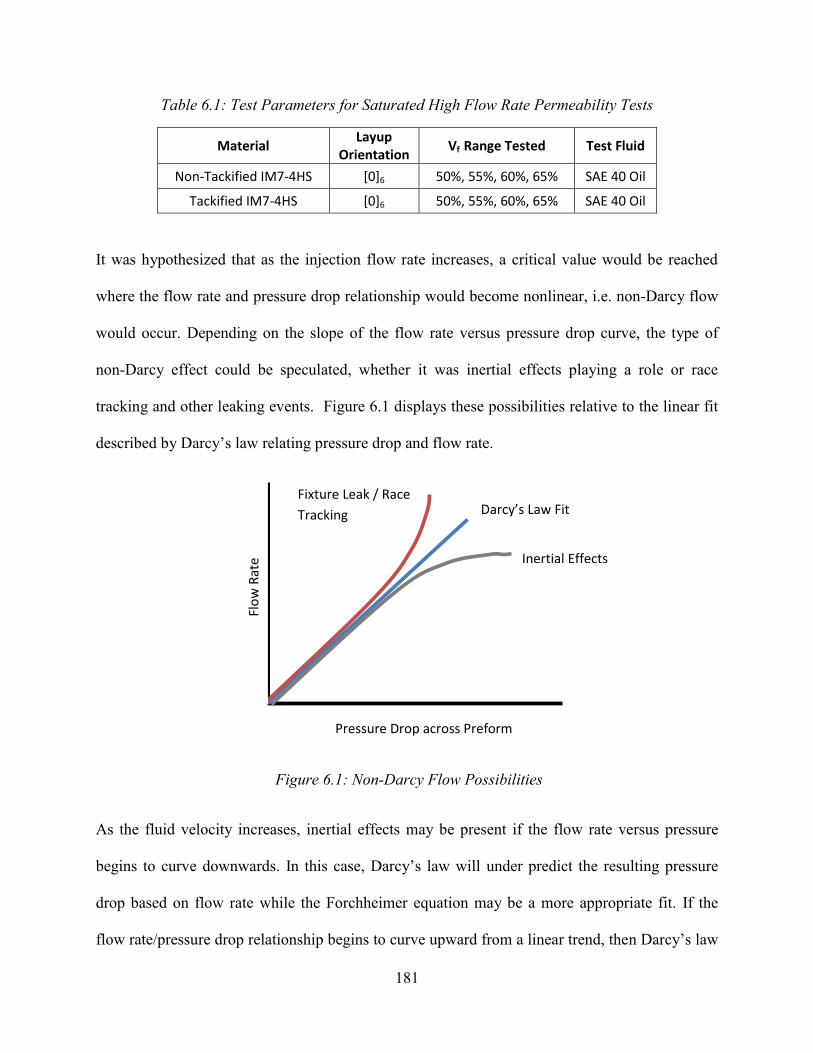
181
Table 6.1: Test Parameters for Saturated High Flow Rate Permeability Tests
Material Layup
Orientation Vf Range Tested Test Fluid
Non-Tackified IM7-4HS [0]6 50%, 55%, 60%, 65% SAE 40 Oil
Tackified IM7-4HS [0]6 50%, 55%, 60%, 65% SAE 40 Oil
It was hypothesized that as the injection flow rate increases, a critical value would be reached
where the flow rate and pressure drop relationship would become nonlinear, i.e. non-Darcy flow
would occur. Depending on the slope of the flow rate versus pressure drop curve, the type of
non-Darcy effect could be speculated, whether it was inertial effects playing a role or race
tracking and other leaking events. Figure 6.1 displays these possibilities relative to the linear fit
described by Darcy’s law relating pressure drop and flow rate.
Figure 6.1: Non-Darcy Flow Possibilities
As the fluid velocity increases, inertial effects may be present if the flow rate versus pressure
begins to curve downwards. In this case, Darcy’s law will under predict the resulting pressure
drop based on flow rate while the Forchheimer equation may be a more appropriate fit. If the
flow rate/pressure drop relationship begins to curve upward from a linear trend, then Darcy’s law
Pressure Drop across Preform
Flo
w R
ate Inertial Effects
Darcy’s Law Fit Fixture Leak / Race
Tracking

182
will over predict the pressure based on flow rate. This may be the result of a pressure leak from
the fixture or fiber washout to the extent of race tracking. These interpretations were used to
describe the result of the IM7-4HS high flow rate tests.
6.3 Results and Discussion
6.3.1 Data Reduction of Previously Measured Permeability
To define an acceptable error value for determination of the critical Forchheimer number,
coefficients of variation of all saturated permeability measurements (including all fiber volume
fractions) from Chapter 4 were averaged. This average coefficient of variation (CV) was 17.43%.
Note that the CV did not change significantly with fiber volume fraction. This amount of scatter,
although high in value, is common in permeability measurements. A recent large-scale effort to
benchmark a permeability measurement procedure produced scatter of ±20% among multiple
researchers’ results for the same preform [69]. Therefore critical error of 17.43% is a reasonable
quantity for the non-Darcy criterion, and any error greater than this this will result in significant
difference from the standard measured scatter. Implementation into Equation 87 resulted in a
critical Forchheimer number of 0.210. Thus, infusions producing Forchheimer numbers higher
than this value should result in a significantly measured non-Darcy effect.
Flow rate versus pressure drop data from the measurements of Chapter 4 for warp aligned,
tackified and non-tackified IM7-4HS were fit to the second-order, Forchheimer equation to
investigate non-Darcy flow. From these re-fits, the Forchheimer permeability and non-Darcy
coefficient were determined, thus ultimately allowing for a critical superficial velocity and flow
rate to be determined. The Forchheimer fit values of the warp aligned non-tackified IM7-4HS
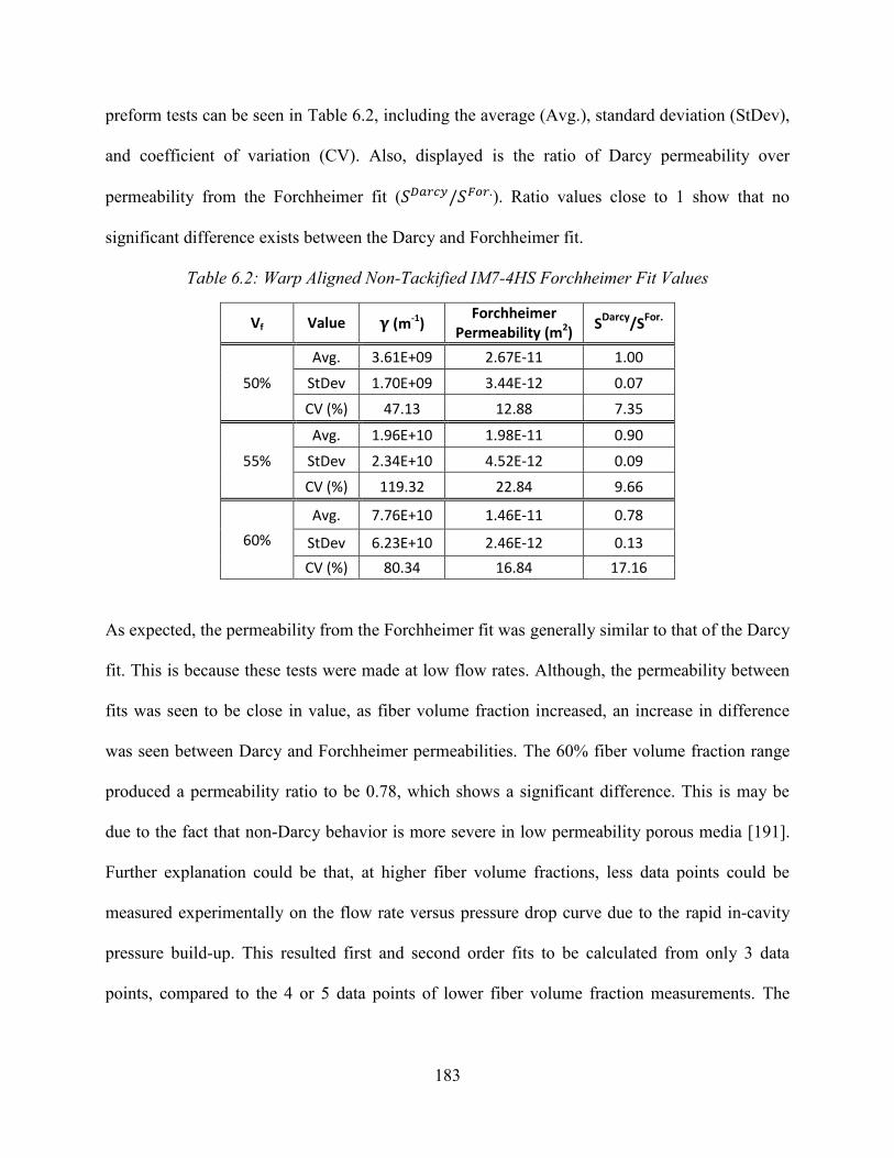
183
preform tests can be seen in Table 6.2, including the average (Avg.), standard deviation (StDev),
and coefficient of variation (CV). Also, displayed is the ratio of Darcy permeability over
permeability from the Forchheimer fit (𝑆𝐷𝑎𝑟𝑐𝑦/𝑆𝐹𝑜𝑟.). Ratio values close to 1 show that no
significant difference exists between the Darcy and Forchheimer fit.
Table 6.2: Warp Aligned Non-Tackified IM7-4HS Forchheimer Fit Values
Vf Value 𝛄 (m-1) Forchheimer
Permeability (m2) S
Darcy/S
For.
50%
Avg. 3.61E+09 2.67E-11 1.00
StDev 1.70E+09 3.44E-12 0.07
CV (%) 47.13 12.88 7.35
55%
Avg. 1.96E+10 1.98E-11 0.90
StDev 2.34E+10 4.52E-12 0.09
CV (%) 119.32 22.84 9.66
60%
Avg. 7.76E+10 1.46E-11 0.78
StDev 6.23E+10 2.46E-12 0.13
CV (%) 80.34 16.84 17.16
As expected, the permeability from the Forchheimer fit was generally similar to that of the Darcy
fit. This is because these tests were made at low flow rates. Although, the permeability between
fits was seen to be close in value, as fiber volume fraction increased, an increase in difference
was seen between Darcy and Forchheimer permeabilities. The 60% fiber volume fraction range
produced a permeability ratio to be 0.78, which shows a significant difference. This is may be
due to the fact that non-Darcy behavior is more severe in low permeability porous media [191].
Further explanation could be that, at higher fiber volume fractions, less data points could be
measured experimentally on the flow rate versus pressure drop curve due to the rapid in-cavity
pressure build-up. This resulted first and second order fits to be calculated from only 3 data
points, compared to the 4 or 5 data points of lower fiber volume fraction measurements. The
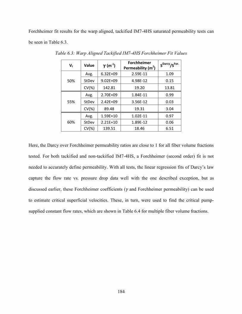
184
Forchheimer fit results for the warp aligned, tackified IM7-4HS saturated permeability tests can
be seen in Table 6.3.
Table 6.3: Warp Aligned Tackified IM7-4HS Forchheimer Fit Values
Vf Value 𝛄 (m-1) Forchheimer
Permeability (m2) SDarcy/SFor.
50%
Avg. 6.32E+09 2.59E-11 1.09
StDev 9.02E+09 4.98E-12 0.15
CV(%) 142.81 19.20 13.81
55%
Avg. 2.70E+09 1.84E-11 0.99
StDev 2.42E+09 3.56E-12 0.03
CV(%) 89.48 19.31 3.04
60%
Avg. 1.59E+10 1.02E-11 0.97
StDev 2.21E+10 1.89E-12 0.06
CV(%) 139.51 18.46 6.51
Here, the Darcy over Forchheimer permeability ratios are close to 1 for all fiber volume fractions
tested. For both tackified and non-tackified IM7-4HS, a Forchheimer (second order) fit is not
needed to accurately define permeability. With all tests, the linear regression fits of Darcy’s law
capture the flow rate vs. pressure drop data well with the one described exception, but as
discussed earlier, these Forchheimer coefficients (𝛾 and Forchheimer permeability) can be used
to estimate critical superficial velocities. These, in turn, were used to find the critical pump-
supplied constant flow rates, which are shown in Table 6.4 for multiple fiber volume fractions.

185
Table 6.4: Critical Velocity and Flow Rate Estimations for Non-Darcy Flow in IM7-4HS with and without Tackifier
Vf = 50%
Flow Rate Value Avg. (cc/min) StDev (cc/min) CV (%)
Non-Tackified IM7-4HS 12.19 9.17 75.21
Tackified IM7-4HS 21.60 19.53 90.42
Vf = 55%
Flow Rate Value Avg. (cc/min) StDev (cc/min) CV (%)
Non-Tackified IM7-4HS 6.22 6.90 110.98
Tackified IM7-4HS 29.90 26.82 89.68
Vf = 60%
Flow Rate Value Avg. (cc/min) StDev (cc/min) CV (%)
Non-Tackified IM7-4HS 0.97 0.60 61.78
Tackified IM7-4HS 27.18 29.44 108.32
For the non-tackified material, the critical flow rates drop as the fiber volume fraction increases.
This is likely because that non-Darcy behavior is becomes more prevalent in low permeability
porous media, as mentioned earlier. However, for the tackified fabric, no clear relationship is
seen between critical flow rate and fiber volume fraction. Regardless of observed trends, the
experimental scatter of the critical flow rates were so large that no reasonable estimation can be
made regarding a critical value. This scatter may best be explained by the experimental
variability seen in the non-Darcy coefficient. This coefficient showed large scatter for both
tackified and non-tackified material, over 100% in some cases (see Table 6.2 and Table 6.3). The
non-Darcy coefficients proved to be very sensitive to the experimental data compared to the
Forchheimer permeability, which was seen to possess standard values of scatter (<20%).
Zeng and Grigg [191] argued for the use of a critical Forchheimer number as a criterion for non-
Darcy flow in porous media. As described by the researchers, the definition of this criterion is

186
simple and can be based on critical error. Unfortunately, the applicability of this method did not
prove consistent, as very large experimental variations were seen in the critical flow rate
estimations. Due to the sensitivity of the calculation of the non-Darcy coefficient, this criterion
cannot be used confidently to find the critical flow rate or velocity values for IM7-4HS preforms.
Nonetheless, further permeability measurements at high flow rates were conducted in attempt to
observe non-Darcy flow. The results of these measurements are discussed next.
6.3.2 High Flow Rate/Pressure Experiments
A total of 8 high flow rate experiments were conducted with tackified and non-tackified IM7-
4HS preforms. These tests were run from 50% fiber volume fraction to 65%. A sample
relationship of the flow rate (𝑄) versus pressure drop (∆𝑃) for a non-tackified IM7-4HS at 50%
fiber volume can be seen in Figure 6.2. It is seen that as the flow rate increases, deviation from a
linear fit was found. This nonlinearity curves upward, as a result of a pressure leak. It was seen
that for this sample, nonlinearity began around flow rate of 7 cc/min and pressure drop of
roughly 690 kPa. At a certain point during testing, when the flow rate was increased over 1.6E-7
m3/s, the measured pressure drop across the preform actually reduced.
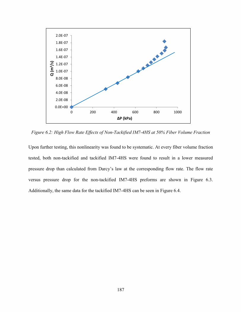
187
Figure 6.2: High Flow Rate Effects of Non-Tackified IM7-4HS at 50% Fiber Volume Fraction
Upon further testing, this nonlinearity was found to be systematic. At every fiber volume fraction
tested, both non-tackified and tackified IM7-4HS were found to result in a lower measured
pressure drop than calculated from Darcy’s law at the corresponding flow rate. The flow rate
versus pressure drop for the non-tackified IM7-4HS preforms are shown in Figure 6.3.
Additionally, the same data for the tackified IM7-4HS can be seen in Figure 6.4.
0.0E+00
2.0E-08
4.0E-08
6.0E-08
8.0E-08
1.0E-07
1.2E-07
1.4E-07
1.6E-07
1.8E-07
2.0E-07
0 200 400 600 800 1000
Q (
m3/s
)
ΔP (kPa)

188
Figure 6.3: Flow Rate versus Pressure Drop for Non-Tackified IM7-4HS
Figure 6.4: Flow Rate versus Pressure Drop for Tackified IM7-4HS
0.0E+00
2.0E-08
4.0E-08
6.0E-08
8.0E-08
1.0E-07
1.2E-07
1.4E-07
1.6E-07
1.8E-07
2.0E-07
0 500 1000 1500 2000
Q (
m3/s
)
ΔP (kPa)
50% Vf
55% Vf
60% Vf
65% Vf
0.0E+00
5.0E-08
1.0E-07
1.5E-07
2.0E-07
2.5E-07
3.0E-07
0 500 1000 1500 2000 2500
Q (
m3/s
)
ΔP (kPa)
50% Vf
55% Vf
60% Vf
65% Vf
189
While these results were interesting, they were not expected from the experiments. Rather than
an appearance of inertial effects, the tests produced signs of fixture leak and race tracking at high
flow rates. The reason for this will be discussed, but notable trends can also be taken from these
figures. For both the non-tackified and tackified preforms, as the fiber volume fraction increased,
higher pressure drops could be achieved before nonlinearity occurred. This results show that high
fiber volume fractions can withstand higher pressures before nonlinearity occurs than low fiber
content preforms. Also, at high fiber volume fractions, low flow rates produce very high pressure
drops compared to high flow rates at low fiber volume fractions.
Further investigation revealed that the non-Darcy flow regime could be attributed to a
combination of the preform type, fiber volume fraction, and the robustness of the fixture. While
running the high flow rate tests, the fixture’s inlet and outlet side cavity thicknesses were
monitored by two LVDTs. It was seen that depending on the fiber volume fraction, the inlet side
of the fixture was pushed upwards once oil pressure increased high enough from flow rate
injection (Figure 6.5). This fixture displacement proved to be significant, and the initiation point
for the nonlinearities seen.

190
Figure 6.5: Fixture Displacement Representation from High Pressure/Flow Rate Testing
A sample LVDT readout of the tackified IM7-4HS high flow rate test at 50% fiber volume
fraction can be seen in Figure 6.6. Here, the LVDT measured cavity depth versus inlet pressure
is plotted over the entire test.
Figure 6.6: Sample LVDT Readout vs. Inlet Pressure for High Pressure/Flow Rate Test at 50% Vf
1.3400
1.3900
1.4400
1.4900
1.5400
1.5900
0 500 1000 1500
LVD
T R
ead
ou
t o
f C
avit
y D
ep
th
(mm
)
Inlet Pressure (kPa)
LVDT Inlet
LVDT Outlet
Compaction Pressure
LVDT
Outlet Inlet Preform High Pressure Inlet Area

191
It can be seen that after the inlet pressure reached roughly 690 kPa (100 psi), the inlet side of the
fixture was displaced upward a significant amount, increasing cavity depth, while the outlet side
of the fixture remained constant. For this specific test, cavity depth at the inlet side increased a
total of 8.9%, which corresponds to a fiber volume fraction decrease of 4%. With this result,
inertial effects are impossible to explore as the apparent robustness of the saturated permeability
fixture is not great enough to withstand high pressure while maintaining constant preform fiber
volume fraction. This critical point of 690 kPa can be seen as the starting point for nonlinear
behavior in the measured flow rate versus pressure drop curve. The corresponding flow rate
versus pressure drop curve for the tackified IM7-4HS preform at 50% can be seen in Figure 6.7.
In this graph, the data points measured before the critical 690 kPa value are marked separately
and are seen to fit well to a linear regression. After this value, Darcy’s law no longer holds as
pressure leaking is observed. Again, this trend was seen for all experiments conducted.
Figure 6.7: Tackified IM7-4HS Flow Rate vs. Pressure Drop with Fixture Displacement Consideration
y = 2E-10x R² = 0.9982
0.0E+00
5.0E-08
1.0E-07
1.5E-07
2.0E-07
2.5E-07
3.0E-07
0 200 400 600 800 1000 1200 1400
Q (
m3/s
)
ΔP (kPa)
Vf = 50%Vf = 50% - Measured Before Fixture Displacement

192
After the high flow rate tests, fiber washout was also seen for the non-tackified preforms. As the
inlet side of the fixture was displaced from oil pressure, the compaction of the preforms (and
fiber volume fraction) was greatly reduced. With low levels of compaction pressure at the inlet
side of the fixture, the non-tackified preforms were loosely held and easily deformed by the
infiltrating flow. Interestingly, the tackified preforms did not exhibit significant signs of fiber
washout. This can be attributed to the added tack and fiber-hold the inter-layer tackifier
provided. Sample post-test state preforms with and without tackifier can be seen in Figure 6.8.
Figure 6.8: Post-test Preform Deformation for (a) Non-Tackified and (b) Tackified IM7-4HS
The addition of tackifier (non-debulked) effectively resists the event of fiber washout and
deformation in the IM7-4HS compared to non-tackified fabric, while also decreasing the
permeability. It should be noted that even without fiber washout, the fixture displacement
became great enough during tackified preform testing to create pressure leaking and non-Darcy
flow. This leads to the conclusion that while tackifier resists fiber washout, the nonlinearities due
to pressure leaking are highly dependent on the fixture’s displacement. Interestingly, at higher
fiber volume fractions, especially at 60% and 65%, higher inlet pressures could be reached
(a) (b)

193
before the fixture was displaced. This can be seen in Figure 6.9, where the inlet LVDT readout
for a tackified preform at 65% is plotted versus the measured inlet pressure.
Figure 6.9: Sample LVDT Readout of Tackified IM7-4HS High Flow Rate Test at 65% Vf
It is clear that significant fixture displacement at the inlet is not measured until the inlet pressure
is over 1400 kPa. Thus, the nonlinearities seen are a function of the inlet pressure reached, the
fixture’s robustness and the applied compaction pressure. It is hypothesized that at the higher
compaction pressures needed to compress the preforms to high volume fractions, the added
compaction aids to resist oil pressure produced at the inlet. Table 6.5 summarizes the critical
inlet pressures reached before fixture displacement occurred at each volume fraction for the
materials tested.
1.08
1.1
1.12
1.14
1.16
1.18
1.2
1.22
1.24
1.26
1.28
0 500 1000 1500 2000 2500
LVD
T R
ead
ou
t o
f C
avit
y D
ep
th (
mm
)
Inlet Pressure (kPa)
LVDT Inlet
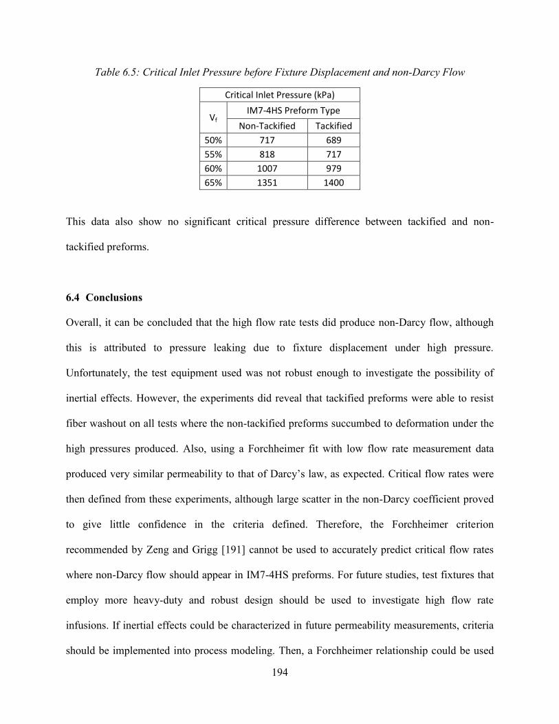
194
Table 6.5: Critical Inlet Pressure before Fixture Displacement and non-Darcy Flow
Critical Inlet Pressure (kPa)
Vf IM7-4HS Preform Type
Non-Tackified Tackified
50% 717 689
55% 818 717
60% 1007 979
65% 1351 1400
This data also show no significant critical pressure difference between tackified and non-
tackified preforms.
6.4 Conclusions
Overall, it can be concluded that the high flow rate tests did produce non-Darcy flow, although
this is attributed to pressure leaking due to fixture displacement under high pressure.
Unfortunately, the test equipment used was not robust enough to investigate the possibility of
inertial effects. However, the experiments did reveal that tackified preforms were able to resist
fiber washout on all tests where the non-tackified preforms succumbed to deformation under the
high pressures produced. Also, using a Forchheimer fit with low flow rate measurement data
produced very similar permeability to that of Darcy’s law, as expected. Critical flow rates were
then defined from these experiments, although large scatter in the non-Darcy coefficient proved
to give little confidence in the criteria defined. Therefore, the Forchheimer criterion
recommended by Zeng and Grigg [191] cannot be used to accurately predict critical flow rates
where non-Darcy flow should appear in IM7-4HS preforms. For future studies, test fixtures that
employ more heavy-duty and robust design should be used to investigate high flow rate
infusions. If inertial effects could be characterized in future permeability measurements, criteria
should be implemented into process modeling. Then, a Forchheimer relationship could be used

195
to govern the flow in a mold fill simulation to account for the additional pressure loss. Further
interesting work would compare non-Darcy flow in saturated versus unsaturated test cases. The
effects of two-phase flow may result in significant difference from that of a saturated case.
196
7. Radial Flow Measurement and Simulation
Infusion visualization methods offer much insight into the flow and permeability characteristics
of reinforcements that closed-mold methods lack. Although closed-mold methods can be used to
determine the principal flow direction with multiple experiments, the sensitivity of the
permeability tensor transformation is high. As discussed in the Saturated Permeability chapter,
slight changes in experimental values produce large swing in the 𝛽 angle determination. Due to
this, a radial visualization fixture was created to verify optically the IM7-4HS fabric principal in-
plane flow directions, while also observing the effects of fabric direction and tackifier. The
following chapter will describe the radial fixture design, method, and results including tackified
vs. non-tackified infusions, 𝛽 angle determination, and transient permeability values. This
chapter will also present simulation results of tackified and non-tackified radial mold fills
produced from the measured permeability data. Inferences can then be made regarding basic
mold fills and the effects of the inter-layer tackifier on preform permeability. This fixture’s
description and infusion results with IM7-4HS preforms can also be found in an earlier published
work by Sommerlot et al. [192].
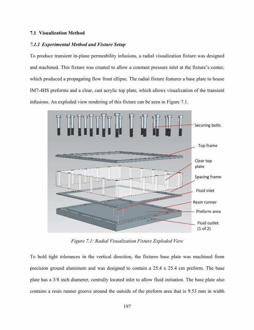
197
7.1 Visualization Method
7.1.1 Experimental Method and Fixture Setup
To produce transient in-plane permeability infusions, a radial visualization fixture was designed
and machined. This fixture was created to allow a constant pressure inlet at the fixture’s center,
which produced a propagating flow front ellipse. The radial fixture features a base plate to house
IM7-4HS preforms and a clear, cast acrylic top plate, which allows visualization of the transient
infusions. An exploded view rendering of this fixture can be seen in Figure 7.1.
Figure 7.1: Radial Visualization Fixture Exploded View
To hold tight tolerances in the vertical direction, the fixtures base plate was machined from
precision ground aluminum and was designed to contain a 25.4 x 25.4 cm preform. The base
plate has a 3/8 inch diameter, centrally located inlet to allow fluid initiation. The base plate also
contains a resin runner groove around the outside of the preform area that is 9.53 mm in width
Securing bolts
Top frame
Clear top plate
Spacing frame
Fluid inlet
Preform area
Fluid outlet (1 of 2)
Resin runner

198
and 3.18 mm deep. The resin runner allows fluid to easily flow to the fixture’s outlets once the
preform area is traversed. This eliminates the unwanted pressure build ups in the fixture and
controls the outer-edge race-tracking. A precision ground aluminum spacing frame sits on the
base plate, which controls the preform thickness. Above that, the 5.08 cm thick, clear acrylic top
plate sits, which is used to compress the preform to the spacing frame thickness. The thickness
of the acrylic top plate ensures little to no flex during compaction and infusion, and therefore
holds a consistent fiber volume fraction throughout testing. A top frame is bolted on to the clear
top plate for added rigidity with 20 equally spaced bolts.
An Airtech Advanced Materials Group pressure pot was used to supply constant pressure
injections to the radial fixture. Injections were set to a target pressure on the pressure pot
regulator, and an in-line pressure transducer (Omega PX180-GV) monitored the exact pressure at
the fixture inlet. The in-line transducer was connected with NI 9219 DAQ board, which was
controlled from a laptop outfitted with LabVIEW. The test fluid used here, again was the SAE 40
motor oil. A Samsung Galaxy Note 10.1 was employed to record infusion from a top viewpoint,
while infusion time was monitored with a stopwatch. After infusions were recorded, the video
images were processed with MATLAB. The MATLAB script allowed the user to manually
select the best fit ellipse of the advancing flow front over time. This allowed calculation of the
radial wet length and orientation (𝛽 angle), which were then used to determine the radial,
unsaturated in-plane permeabilities following the formulation of Weitzenböck et al. [81], [193]
for anisotropic media. The processed images of the advancing ellipses were averaged over the
infusion time for principal orientation and in-plane permeabilities. The MATLAB script used for
this processing can be found in Appendix C. Constant pressure injections were made at a target
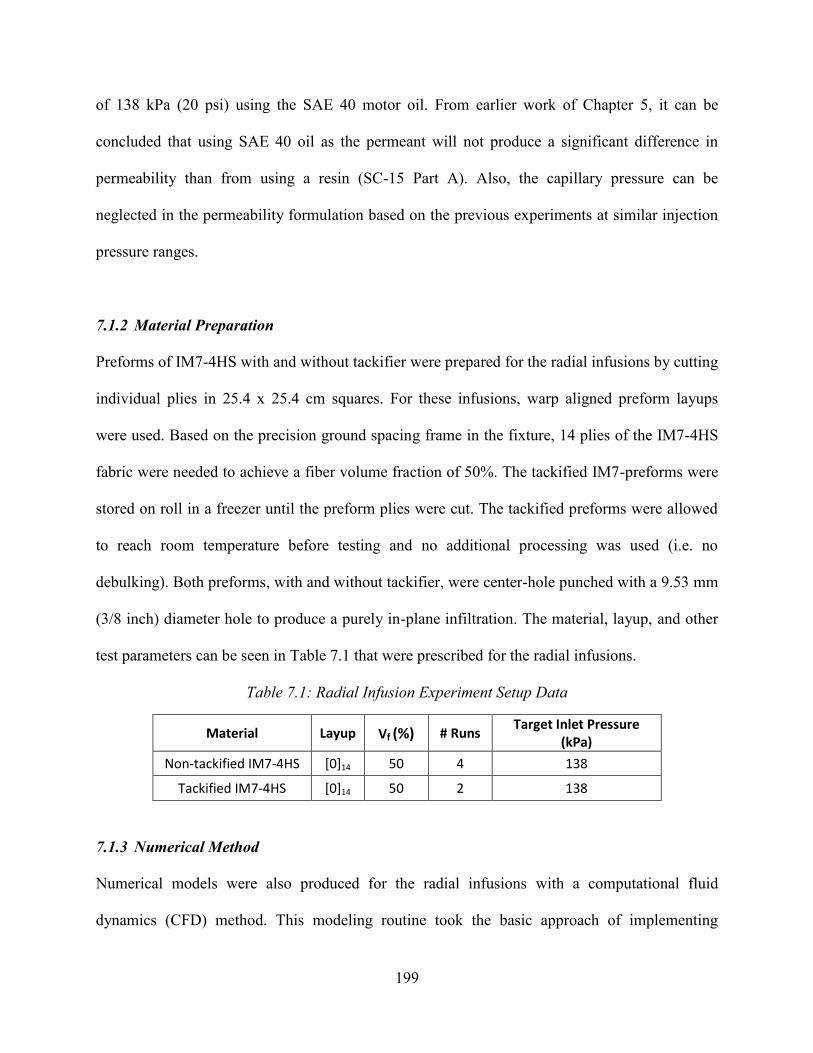
199
of 138 kPa (20 psi) using the SAE 40 motor oil. From earlier work of Chapter 5, it can be
concluded that using SAE 40 oil as the permeant will not produce a significant difference in
permeability than from using a resin (SC-15 Part A). Also, the capillary pressure can be
neglected in the permeability formulation based on the previous experiments at similar injection
pressure ranges.
7.1.2 Material Preparation
Preforms of IM7-4HS with and without tackifier were prepared for the radial infusions by cutting
individual plies in 25.4 x 25.4 cm squares. For these infusions, warp aligned preform layups
were used. Based on the precision ground spacing frame in the fixture, 14 plies of the IM7-4HS
fabric were needed to achieve a fiber volume fraction of 50%. The tackified IM7-preforms were
stored on roll in a freezer until the preform plies were cut. The tackified preforms were allowed
to reach room temperature before testing and no additional processing was used (i.e. no
debulking). Both preforms, with and without tackifier, were center-hole punched with a 9.53 mm
(3/8 inch) diameter hole to produce a purely in-plane infiltration. The material, layup, and other
test parameters can be seen in Table 7.1 that were prescribed for the radial infusions.
Table 7.1: Radial Infusion Experiment Setup Data
Material Layup Vf (%) # Runs Target Inlet Pressure
(kPa)
Non-tackified IM7-4HS [0]14 50 4 138
Tackified IM7-4HS [0]14 50 2 138
7.1.3 Numerical Method
Numerical models were also produced for the radial infusions with a computational fluid
dynamics (CFD) method. This modeling routine took the basic approach of implementing

200
experimental permeability values into a prescribed modeled preform region. The entire domain
consisted of the 3D preform and resin runner regions. The preform was designated as a porous
media with in-plane permeabilities defined from the experimental radial infusion results, and a
through-thickness permeability defined from the saturated experimental results described in
Chapter 4. The resin runner region was prescribed as general void space. Boundary conditions
matched those of the experiments including a central pressure inlet, atmospheric outlets, and wall
boundaries around the resin runner. A volume of fluid (VOF) method was employed where
modeled fluid was injected into the domain, displacing the initially prescribed air-filled mold.
With this approach, the fluid volume fraction is tracked as the flow front progresses in time
steps. The he equations are solved in this case using the VOF method. The model is composed of
the continuity equation given by Equation 88, where 𝜌 is density, 𝑡 is the time and 𝑣 is the local
velocity.
𝜕𝜌
𝜕𝑡+ ∇ ∙ (𝜌𝑣) = 0 (88)
The permeating fluid volume fraction is given by Equation 89, where 𝑉𝑓 is the volume fraction.
𝜕𝑉𝑓
𝜕𝑡+ ∇ ∙ (𝑉𝑓𝑣) = 0 (89)
The momentum equation for each volume is given by Equation 90, where 𝜏𝑖𝑗 is the stress tensor,
𝜇 is the fluid viscosity, 𝑔 is the gravity, 𝑃 is the pressure, and 𝐹 is an external source vector that
can be used to incorporate the resistive force from the porous media.
𝜕(𝜌𝑣)
𝜕𝑡+ ∇ ∙ (𝜌𝑣𝑣) = −∆𝑃 + ∇ ∙ (𝜇𝜏𝑖𝑗) + 𝜌𝑔 + 𝐹 (90)
A simple mesh refinement study was also performed, as meshed domains of both 1,225 and
390,000 elements were solved with the described VOF method.

201
7.2 Results and Discussion
7.2.1 Experimental Results
A sample MATLAB processed image of an advancing flow front is shown in Figure 7.2. Here,
the IM7-4HS preform’s warp (0°) and weft (90°) directions are noted and the best fit ellipse can
be seen, which was created from the user defined points. The first and second principal axes are
also defined, while 𝛽 is shown as the angle between the warp and 𝑆11 direction. The major and
minor axes of the flow front also can be seen, as well a principal orientation based on the fabric
0° or warp direction. These axes lengths were scaled and inputted as radial wet lengths for the
radial permeability calculation from Weitzenböck et al. [81], [193]. The recorded stopwatch time
in the image was also inputted into the formulation. The exact values of the parameters including
𝑆𝑥𝑥, 𝑆𝑦𝑦, the principal permeabilities, and 𝛽 angle are then outputted from the MATLAB script.
Figure 7.2: Sample MATALB Processed Radial Infusion Image

202
Although the permeability and 𝛽 angle were averaged over the entire infusion for each run, the
image processed results can be plotted over time. In Figure 7.3, sample data from a non-tackified
preform is seen where both the 𝑆11 and 𝑆22 permeabilities and 𝛽 are plotted on the same graph
over time.
Figure 7.3: Sample Unsaturated Radial Permeability and 𝛽 Angle over Infusion Time
Here, the calculated permeabilities and orientation angle all show stability over time. This can be
attributed to consistent preform geometry and test parameters. The averaged values from all the
runs are displayed in Table 7.2. This includes the first and second principal permeabilities as
well as the angle of orientation of first principal permeability. Following in Table 7.3, the warp,
weft, and 45° off-axis permeabilities can be seen. These permeabilities were calculated from
rotations of the best fit ellipse of each run.
0.00
30.00
60.00
90.00
120.00
1E-12
1.1E-11
2.1E-11
3.1E-11
4.1E-11
5.1E-11
6.1E-11
7.1E-11
8.1E-11
0 100 200 300 400 500 600 700
β (
°)
Un
satu
rate
d P
erm
eab
ility
(m
2)
Time (s)
S11S22β

203
Table 7.2: Radial Unsaturated Principal Permeability Results
Run S11 (m
2) S22 (m2) 𝜷 (°)
Non-tackified
Tackified Non-
tackified Tackified
Non-tackified
Tackified
1 6.51E-11 2.56E-11 1.83E-11 2.05E-11 91.23 -7.52
2 2.71E-11 7.01E-12 1.48E-11 6.55E-12 92.68 113.68
3 2.05E-11 - 1.22E-11 - 98.84 -
4 2.55E-11 - 1.06E-11 - 90.07 -
Avg. 3.46E-11 1.63E-11 1.40E-11 1.35E-11 93.21 53.08
StDev 2.06E-11 - 3.38E-12 - 3.91 -
CV (%) 59.48 - 24.16 - 4.19 -
Table 7.3: Radial Unsaturated Warp, Weft, and Off-axis Permeability Results
Run Sxx Syy Sxx'
Non-tackified
Tackified Non-
tackified Tackified
Non-tackified
Tackified
1 1.83E-11 2.55E-11 6.50E-11 2.06E-11 2.93E-11 2.34E-11
2 1.48E-11 6.60E-12 2.71E-11 6.95E-12 1.97E-11 7.01E-12
3 1.23E-11 - 2.02E-11 - 1.66E-11 -
4 1.06E-11 - 2.55E-11 - 1.50E-11 -
Avg 1.40E-11 1.60E-11 3.44E-11 1.38E-11 2.01E-11 1.52E-11
StDev 3.36E-12 - 2.06E-11 - 6.41E-12 -
CV (%) 23.97 - 59.82 - 31.87 -
Interestingly, the first run for both the tackified and non-tackified preforms showed much higher
permeabilities than the subsequent runs. A specific reason for this is not certain. Aside from this
artifact, important inferences can be made. Even with the first runs producing higher
permeability, the shape of the flow front ellipses remained constant. The non-tackified warp
aligned IM7-4HS preforms were seen to show a strong bias in permeability in the weft direction.
This is seen as the 𝛽 angle was calculated to be nearly 90° for every run made. Alternatively, the
tackified warp aligned preforms showed little directional bias, with warp, weft, and off-axis
permeability measurements all being similar in value. The 𝛽 values here showed very scattered
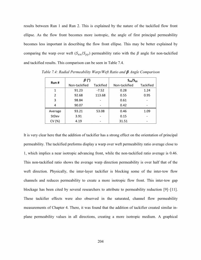
204
results between Run 1 and Run 2. This is explained by the nature of the tackified flow front
ellipse. As the flow front becomes more isotropic, the angle of first principal permeability
becomes less important in describing the flow front ellipse. This may be better explained by
comparing the warp over weft (𝑆𝑥𝑥/𝑆𝑦𝑦) permeability ratio with the 𝛽 angle for non-tackified
and tackified results. This comparison can be seen in Table 7.4.
Table 7.4: Radial Permeability Warp/Weft Ratio and 𝜷 Angle Comparison
Run # 𝜷 (°) Sxx/Syy
Non-tackified Tackified Non-tackified Tackified
1 91.23 -7.52 0.28 1.24
2 92.68 113.68 0.55 0.95
3 98.84 - 0.61 -
4 90.07 - 0.42 -
Average 93.21 53.08 0.46 1.09
StDev 3.91 - 0.15 -
CV (%) 4.19 - 31.51 -
It is very clear here that the addition of tackifier has a strong effect on the orientation of principal
permeability. The tackified preforms display a warp over weft permeability ratio average close to
1, which implies a near isotropic advancing front, while the non-tackified ratio average is 0.46.
This non-tackified ratio shows the average warp direction permeability is over half that of the
weft direction. Physically, the inter-layer tackifier is blocking some of the inter-tow flow
channels and reduces permeability to create a more isotropic flow front. This inter-tow gap
blockage has been cited by several researchers to attribute to permeability reduction [9]–[11].
These tackifier effects were also observed in the saturated, channel flow permeability
measurements of Chapter 4. There, it was found that the addition of tackifier created similar in-
plane permeability values in all directions, creating a more isotropic medium. A graphical
205
comparison of the average saturated, channel flow measurements of the warp aligned IM7-4HS
is made with the average radial unsaturated permeabilities in Figure 7.4.
Figure 7.4: Average IM7-4HS Permeability Comparison of Radial Unsaturated and Saturated Channel Flow Measurements
Very similar relationships between the radial and channel flow measurements can be seen over
the test direction. Tackified preforms showed little change over test direction in both saturated
and radial unsaturated experiments, while the non-tackified preforms show an increasing bias
towards the 90° direction. It should be noted that the radial unsaturated permeabilities tested 40%
to 50% lower than their saturated counterparts. This relationship has also been noted by Estrada
et al. [11], who found up to ~45% reduction in unsaturated permeability compared to saturated
test cases with 4 wt% tackified preforms. This, although, is in contradiction from the channel
flow unsaturated results of Chapter 5, where no significant difference was seen between
unsaturated and saturated permeabilities. Explanation for this must then be placed on the
difference between radial and channel flow test parameters. Lundström et al. [67], in a round
1.00E-12
1.10E-11
2.10E-11
3.10E-11
4.10E-11
5.10E-11
6.10E-11
7.10E-11
Sxx [0°] Sxx' [45°] Syy [90°]
Pe
rme
abili
ty (
m2)
Test Direction
Non-tackified (Radial Unsaturated)Tackified (Radial Unsaturated)Non-tackified (Saturated)Tackified (Saturated)

206
robin permeability study, reported that radial flow methods produced permeability values up
23% lower than parallel flow techniques for the same preform. They also explained that radial
flow techniques suffers from several sources of error that are not present in channel flow tests,
including deviations of the inlet hole shape, the inlet hole radius, and the local permeability near
the inlet. With this in consideration, radial flow measurement techniques may represent a higher
probability of experimental scatter compared to parallel flow techniques. This may also explain
why both the saturated and unsaturated channel flow measurements of Chapter 5 produced very
similar permeabilities for the IM7-4HS preforms, while the current radial technique produced
very different results.
7.2.2 Comparison with Numerical Solution
To demonstrate the applicability of permeability measurements to simulate mold fills, the
permeability results from the first run of the experiments with and without tackifier were used to
generate numerical mold fill solutions. A three-dimensional model was constructed of the mold
geometry as described in the methods section of this chapter. Numerical simulations results were
produced with two in-plane permeability experimental measurements (𝑆𝑥𝑥 and 𝑆𝑦𝑦) and a
transverse permeability measurement, which was presented in Chapter 4. Numerical simulation
results are compared against actual infusions images at the same time step for both non-tackified
and tackified IM7-4HS preforms in Figure 7.5 and Figure 7.6, respectively. The results are
divided in three columns: (A) experimental advancing flow fronts that are image processed
displaying the best fit ellipse, (B) numerical flow fronts found from a coarsely meshed domain of
1,225 elements, and (C) numerical flow fronts from a refined domain meshed with 390,000
elements. Each column of results represents the flow front ellipse at the infusion time displayed

207
in the bottom left of the images in column (A). Four time intervals images were selected to be
displayed.
Figure 7.5: Non-Tackified IM7-4HS Advancing Flow Front Comparisons. (A) MATLAB processed experimental flow front propagation with best fit ellipse. (B) Rough mesh numerical advancing front solutions. (C) Fine mesh numerical advancing front solutions. Numerical solutions display volume fraction of the test fluid, SAE 40 oil (red) displacing air (blue).
(A) (B) (C)
t = 1 min
t = 2 min
t = 4 min
t = 6 min
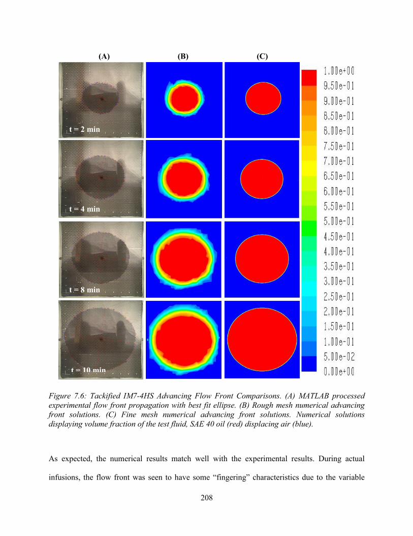
208
Figure 7.6: Tackified IM7-4HS Advancing Flow Front Comparisons. (A) MATLAB processed experimental flow front propagation with best fit ellipse. (B) Rough mesh numerical advancing front solutions. (C) Fine mesh numerical advancing front solutions. Numerical solutions displaying volume fraction of the test fluid, SAE 40 oil (red) displacing air (blue).
As expected, the numerical results match well with the experimental results. During actual
infusions, the flow front was seen to have some “fingering” characteristics due to the variable
t = 2 min
t = 4 min
t = 8 min
(A) (B) (C)
t = 10 min

209
porosity produced from the fabric geometry (including inter-tow and intra-tow porosities). These
results are not seen in the numerical simulations, as the preforms were modeled as porous media
of known permeability rather than geometrical representations of the fabric architecture.
A simple numerical mesh refinement study was conducted and the results were shown. Coarsely
meshed geometries were run with 1,225 elements and compared with a fine mesh refinement of
319,000 elements. The total fill time was mostly time step dependent and not iteration
dependent, so the simulation time was similar for the coarse and fine mesh cases. The resolution
of the flow front boundary was much better for the fine mesh because of the ability to more
accurately position the volume fraction of fluid in a smaller computational cell. The time step
was chosen as 1E-3s to start the simulation and once the simulation was advancing steadily an
adaptive time step was adopted to simulate the advancing flow front more rapidly while
continuing to keep good convergence.
The simulations for both non-tackified and tackified cases were also run to investigate the resin
runner effect on each mold fill case. Numerical solutions displaying these results can be seen for
the non-tackified IM7-4HS sample in Figure 7.7, while Figure 7.8 shows a similar set of results
for the tackified IM7-4HS sample. Both figures contain 4 images labeled (A)-(F) showing the
volume fraction of the permeating test fluid displacing air in the mold at selected time steps.
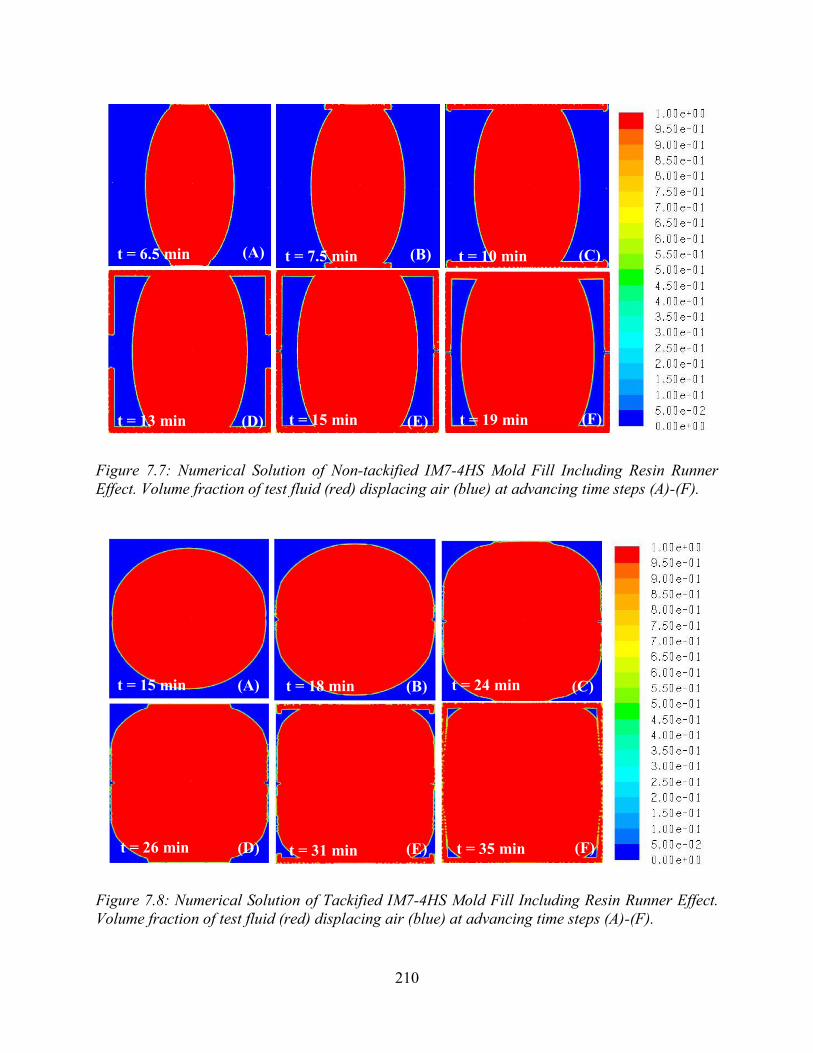
210
Figure 7.7: Numerical Solution of Non-tackified IM7-4HS Mold Fill Including Resin Runner Effect. Volume fraction of test fluid (red) displacing air (blue) at advancing time steps (A)-(F).
Figure 7.8: Numerical Solution of Tackified IM7-4HS Mold Fill Including Resin Runner Effect. Volume fraction of test fluid (red) displacing air (blue) at advancing time steps (A)-(F).
(F) t = 19 min
(A) (B) (C)
(D) (E)
t = 6.5 min t = 7.5 min t = 10 min
t = 13 min t = 15 min
(A) (B) (C)
(D) (E) (F)
t = 15 min t = 18 min t = 24 min
t = 26 min t = 31 min t = 35 min
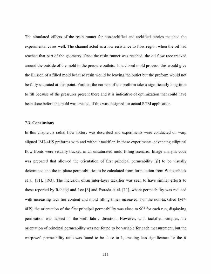
211
The simulated effects of the resin runner for non-tackified and tackified fabrics matched the
experimental cases well. The channel acted as a low resistance to flow region when the oil had
reached that part of the geometry. Once the resin runner was reached, the oil flow race tracked
around the outside of the mold to the pressure outlets. In a closed mold process, this would give
the illusion of a filled mold because resin would be leaving the outlet but the preform would not
be fully saturated at this point. Further, the corners of the preform take a significantly long time
to fill because of the pressures present there and it is indicative of optimization that could have
been done before the mold was created, if this was designed for actual RTM application.
7.3 Conclusions
In this chapter, a radial flow fixture was described and experiments were conducted on warp
aligned IM7-4HS preforms with and without tackifier. In these experiments, advancing elliptical
flow fronts were visually tracked in an unsaturated mold filling scenario. Image analysis code
was prepared that allowed the orientation of first principal permeability (𝛽) to be visually
determined and the in-plane permeabilities to be calculated from formulation from Weitzenböck
et al. [81], [193]. The inclusion of an inter-layer tackifier was seen to have similar effects to
those reported by Rohatgi and Lee [6] and Estrada et al. [11], where permeability was reduced
with increasing tackifier content and mold filling times increased. For the non-tackified IM7-
4HS, the orientation of the first principal permeability was close to 90° for each run, displaying
permeation was fastest in the weft fabric direction. However, with tackified samples, the
orientation of principal permeability was not found to be variable for each measurement, but the
warp/weft permeability ratio was found to be close to 1, creating less significance for the 𝛽
212
angle. Notably, this effect was also seen from the saturated parallel flow experiments presented
in Chapter 4. Also, the tackified IM7-4HS exhibited more isotropic flow front ellipses (more
circular) than the non-tackified samples. This effect is attributed to the tackifier blocking the
flow channels between tows throughout the fabric, creating a more uniform advancing flow front
than those that are subject only to the anisotropic fabric architecture (i.e. non-tackified flow
fronts). Interestingly, much like the results in Chapter 4, the permeability was reduced more
significantly in the weft fabric direction than the warp. It should be noted that the radial
unsaturated measurements produced permeabilities much lower than saturated and unsaturated
parallel flow measurements of Chapter 4 and 5, respectively. Permeability measurements from
radial flow techniques have also been reported by researchers to be lower compared to parallel
flow measurements of the same preform, while additional sources of error have been discussed
to be at play in the radial technique [67]. Thus, the radial flow method, while being very useful
in quickly defining the full in-plane permeability tensor and 𝛽 angle, may be less reliable than
the channel flow techniques for determining permeability.
Numerical mold fill models of both the tackified and non-tackified IM7-4HS were also produced
using the experimentally measured permeability values. The models displayed good correlation
between experimental and numerical mold fills and also were used to display effects seen from
resin runners. The effect of tackifier points to need for characterization of such materials for
accurate mold fill modeling in LCM. The presence of tackifier can not only change preform
permeability, it can significantly alter the advancing front shape or flow profile of the infiltrating
resin. Future work would involve validating these measurements and conclusions for the IM7-
4HS material on a complex geometry mold fill. Also, to expand this work further for composite

213
manufacturing modeling, a method of geometrical characterization of the tackified fabric should
be developed so that CFD can be used to predict the permeability through a known geometry,
alleviating the need for experimental work.
214
8. Summary and Conclusions
8.1 Summary and Conclusions
In this study, a compaction and permeability characterization of a four harness satin carbon
fabric (IM7-4HS) with and without a unique low areal weight inter-layer tackifier (Cytec
CYCOM PR 520-1) was conducted. Characterization included dry and wetted compaction
experiments, saturated in-plane and through-thickness permeability measurements, high flow
rate saturated measurements, unsaturated parallel flow measurements, and radial flow
unsaturated measurements. These characterization methods were used to investigate the effects
of tackifier, preform debulking, preform layup, saturation, flow rate, capillary pressure, and fluid
type on the processing for LCM and RTM applications. Further novel contributions in this study
include results on the effect of tackifier on principal permeability orientation, a modified
experimental capillary pressure technique for permeability correction, and an investigation on the
applicability of a specific criterion for defining non-Darcy flow in high flow rate permeability
measurements.
Specifically, the investigations revealed that the addition of the inter-layer tackifier significantly
reduced the permeability of IM7-4HS preforms compared to non-tackified samples, while
compaction was less affected. Tackifier also significantly altered the orientation of the principal
in-plane permeabilities. Additional processing of tackified fabric under heat and pressure cured
the tackifier to produce debulked preforms. These debulked samples were very stiff and provided
large resistance to compaction pressures and nesting. Consequently, debulked preforms produced
an interesting behavior in permeability, where the resisted fiber nesting characteristic provided

215
larger inter-tow flow channels than unprocessed tackified samples. This resulted in
permeabilities generally higher than the unprocessed tackified samples and similar to the non-
tackified material for both in-plane and transverse flow directions. Additionally, it was found
that the directional biases of the in-plane permeability tensor could be tailored by altering the
preform layup stacking sequence.
Further investigations compared unsaturated parallel flow permeability measurements with oil
and a low-viscosity epoxy resin. It was found that fluid type had little effect on permeability on
the non-tackified preforms, unless injection pressure was very low where capillary pressures are
significant. However, the tackified preforms showed a large sensitivity to the fluid type, and it
was hypothesized that the addition of tackifier alters the wettability of the fiber reinforcement
depending on fluid type, and also encourages more intra-tow flow, which increases capillary
action. Additional high flow rate testing showed the possibility of non-Darcy flow during
infusions. From these results, it was concluded that all LCM infusions should be considered
based on fluid velocity or flow rate. Depending on the velocity, capillary pressures may be
significant or neglected, inertial effects may require a Forchheimer relationship to describe the
flow, or Darcy’s law may fit the application well.
For consideration of RTM and other LCM applications, the use of tackifier strongly aids in
preforming, holding fiber orientation and part shape, and resisting deformation in high pressure
or flow rate infusions. Although, the addition of tackifier will also reduce permeability and
increase mold fill times. Debulking can further hold preform shape as the cured tackifier fuses
the reinforcement fiber network together. However, the mold used must be robust enough to

216
overcome the large resistance to compaction the debulked preform provides. Also, if debulking
is considered, the injection resin should be chemically compatible, if not the same, as the
tackifier system to avoid void formations, poor fiber/matrix interfaces, and ultimately low part
performance.
8.2 Future Work
For a more robust characterization of the IM7-4HS preforms, specialized test fixtures should be
produced to measure permeability of deformed geometry native to complex molds, including
sheared and curved portions of the reinforcement. Further investigations should be made to
quantify the void formation in IM7-4HS preforms with and without the inter-layer tackifier, as
well as in the debulked preforms after infusions. Aside from the tackifier showing aid in preform
creation, the addition of tackifier, especially pre-cured in the debulk process, may result in
irregular flows and local blockages leading to possible void formations. To further investigate
the high flow rate experiments, unsaturated infusions should be investigated with a robust fixture
that will not permit displacement or race-tracking. Also, a visualization window should be
introduced so that the precise pressure or flow rate can be defined where fiber shift and washout
initiate for non-tackified and tackified preforms. This would be of very practical interest for
RTM applications and material selection consideration.
While this study has shown the applicability of permeability measurements to simple numerical
mold fill solutions, further work should look to predict permeability based on geometry and other
infusion parameters. This would alleviate the need for expensive, time consuming manual
characterization techniques. Furthermore, the physical geometry of tackifier should be modeled

217
to predict the altered flow and permeability through tackified fabrics. These permeability
solutions could then be implemented into Darcian flow based solver for mold fill solutions.
Ultimately, a unified reinforcement draping and resin flow simulation tool would create an
efficient and ideal approach to process modeling. Here, reinforcement geometry could be used as
the input while nesting, shear, and other deformations induced from preforming could be solved
mechanically. Then, with the altered preform geometry and infusion parameters known, the
permeating flow could be simulated with computational fluid dynamics. This would be a
powerful tool for process modeling, although further manual characterization must be done
before this technology is computationally available.

218
APPENDICES
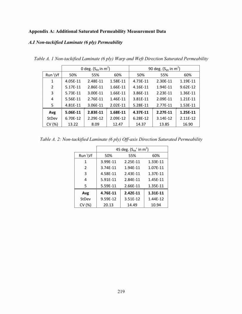
219
Appendix A: Additional Saturated Permeability Measurement Data
A.I Non-tackified Laminate (6 ply) Permeability
Table A. 1 Non-tackified Laminate (6 ply) Warp and Weft Direction Saturated Permeability
0 deg. (Sxx in m2) 90 deg. (Syy in m2)
Run \Vf 50% 55% 60% 50% 55% 60%
1 4.05E-11 2.48E-11 1.58E-11 4.73E-11 2.30E-11 1.19E-11
2 5.17E-11 2.86E-11 1.66E-11 4.16E-11 1.94E-11 9.62E-12
3 5.73E-11 3.00E-11 1.66E-11 3.86E-11 2.23E-11 1.36E-11
4 5.56E-11 2.76E-11 1.46E-11 3.81E-11 2.09E-11 1.21E-11
5 4.81E-11 3.06E-11 2.02E-11 5.28E-11 2.77E-11 1.53E-11
Avg 5.06E-11 2.83E-11 1.68E-11 4.37E-11 2.27E-11 1.25E-11
StDev 6.70E-12 2.29E-12 2.09E-12 6.28E-12 3.14E-12 2.11E-12
CV (%) 13.22 8.09 12.47 14.37 13.85 16.90
Table A. 2: Non-tackified Laminate (6 ply) Off-axis Direction Saturated Permeability
45 deg. (Sxx’ in m2)
Run \Vf 50% 55% 60%
1 3.99E-11 2.25E-11 1.33E-11
2 3.74E-11 1.94E-11 1.07E-11
3 4.58E-11 2.43E-11 1.37E-11
4 5.91E-11 2.84E-11 1.45E-11
5 5.59E-11 2.66E-11 1.35E-11
Avg 4.76E-11 2.42E-11 1.31E-11
StDev 9.59E-12 3.51E-12 1.44E-12
CV (%) 20.13 14.49 10.94

220
Table A. 3: Non-tackified Laminate (6 ply) Principal Saturated Permeability
S11 (1st Principal Permeability in m2) S22 (2nd Principal Permeability in m2)
Run \Vf 50% 55% 60% 50% 55% 60%
1 4.92E-11 2.56E-11 1.59E-11 3.87E-11 2.22E-11 1.18E-11
2 5.72E-11 3.05E-11 1.74E-11 3.61E-11 1.75E-11 8.87E-12
3 5.75E-11 3.04E-11 1.72E-11 3.84E-11 2.19E-11 1.30E-11
4 6.19E-11 2.96E-11 1.50E-11 3.18E-11 1.89E-11 1.17E-11
5 5.64E-11 3.21E-11 2.27E-11 4.45E-11 2.62E-11 1.28E-11
Avg 5.64E-11 2.96E-11 1.76E-11 3.79E-11 2.13E-11 1.16E-11
StDev 4.60E-12 2.45E-12 2.97E-12 4.61E-12 3.37E-12 1.67E-12
CV (%) 8.16 8.26 16.86 12.17 15.80 14.33
Table A. 4: Non-tackified Laminate (6 ply) Through-thickness Saturated Permeability
Through-thickness (Szz in m2)
Vf Run 1 Run 2 Run 3 Run 4 Run5 Avg. StDev CV (%)
50% 1.43E-
12 1.49E-
12 1.51E-
12 2.08E-
12 2.01E-
12 1.70E-12 3.15E-13 18.53
55% 7.71E-
13 8.40E-
13 7.31E-
13 1.01E-
12 1.09E-
12 8.89E-13 1.56E-13 17.56
60% 3.76E-
13 4.40E-
13 3.78E-
13 5.26E-
13 6.24E-
13 4.69E-13 1.06E-13 22.66
A.II Debulked Laminate (6 ply) Permeability
Table A. 5: Debulked Laminate (6 ply) Warp and Weft Direction Saturated Permeability
0 deg. (Sxx in m2) 90 deg. (Syy in m2)
Run \Vf 50% 55% 60% 50% 55% 60%
1 3.39E-11 2.24E-11 1.54E-11 9.42E-11 2.67E-11 8.45E-12
2 6.15E-11 2.45E-11 1.06E-11 5.55E-11 2.24E-11 9.76E-12
3 7.39E-11 2.72E-11 1.09E-11 6.07E-11 1.69E-11 5.25E-12
4 3.51E-11 1.62E-11 7.99E-12 9.46E-11 3.42E-11 1.35E-11
5 3.20E-11 1.76E-11 1.02E-11 4.95E-11 2.15E-11 1.00E-11
Avg. 4.73E-11 2.16E-11 1.10E-11 7.09E-11 2.43E-11 9.39E-12
StDev 1.92E-11 4.63E-12 2.70E-12 2.18E-11 6.52E-12 2.98E-12
CV (%) 40.61 21.43 24.53 30.75 26.78 31.69
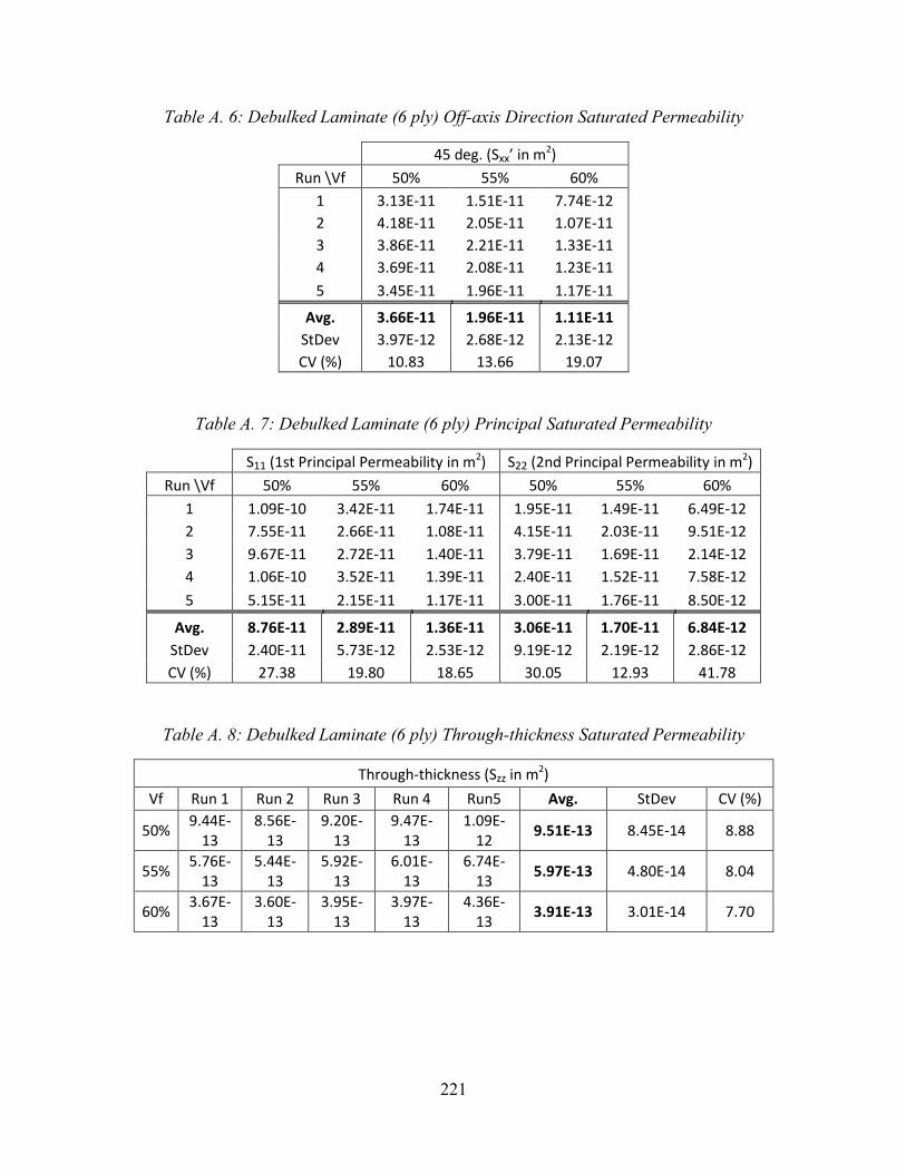
221
Table A. 6: Debulked Laminate (6 ply) Off-axis Direction Saturated Permeability
45 deg. (Sxx’ in m2)
Run \Vf 50% 55% 60%
1 3.13E-11 1.51E-11 7.74E-12
2 4.18E-11 2.05E-11 1.07E-11
3 3.86E-11 2.21E-11 1.33E-11
4 3.69E-11 2.08E-11 1.23E-11
5 3.45E-11 1.96E-11 1.17E-11
Avg. 3.66E-11 1.96E-11 1.11E-11
StDev 3.97E-12 2.68E-12 2.13E-12
CV (%) 10.83 13.66 19.07
Table A. 7: Debulked Laminate (6 ply) Principal Saturated Permeability
S11 (1st Principal Permeability in m2) S22 (2nd Principal Permeability in m2)
Run \Vf 50% 55% 60% 50% 55% 60%
1 1.09E-10 3.42E-11 1.74E-11 1.95E-11 1.49E-11 6.49E-12
2 7.55E-11 2.66E-11 1.08E-11 4.15E-11 2.03E-11 9.51E-12
3 9.67E-11 2.72E-11 1.40E-11 3.79E-11 1.69E-11 2.14E-12
4 1.06E-10 3.52E-11 1.39E-11 2.40E-11 1.52E-11 7.58E-12
5 5.15E-11 2.15E-11 1.17E-11 3.00E-11 1.76E-11 8.50E-12
Avg. 8.76E-11 2.89E-11 1.36E-11 3.06E-11 1.70E-11 6.84E-12
StDev 2.40E-11 5.73E-12 2.53E-12 9.19E-12 2.19E-12 2.86E-12
CV (%) 27.38 19.80 18.65 30.05 12.93 41.78
Table A. 8: Debulked Laminate (6 ply) Through-thickness Saturated Permeability
Through-thickness (Szz in m2)
Vf Run 1 Run 2 Run 3 Run 4 Run5 Avg. StDev CV (%)
50% 9.44E-
13 8.56E-
13 9.20E-
13 9.47E-
13 1.09E-
12 9.51E-13 8.45E-14 8.88
55% 5.76E-
13 5.44E-
13 5.92E-
13 6.01E-
13 6.74E-
13 5.97E-13 4.80E-14 8.04
60% 3.67E-
13 3.60E-
13 3.95E-
13 3.97E-
13 4.36E-
13 3.91E-13 3.01E-14 7.70
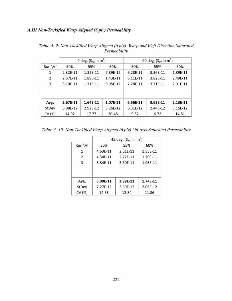
222
A.III Non-Tackified Warp Aligned (6 ply) Permeability
Table A. 9: Non-Tackified Warp Aligned (6 ply) Warp and Weft Direction Saturated Permeability
0 deg. (Sxx in m2) 90 deg. (Syy in m2)
Run \Vf 50% 55% 60% 50% 55% 60%
1 2.32E-11 1.32E-11 7.89E-12 6.28E-11 3.36E-11 1.89E-11
2 2.57E-11 1.89E-11 1.43E-11 6.11E-11 3.82E-11 2.49E-11
3 3.10E-11 1.71E-11 9.95E-12 7.28E-11 3.71E-11 2.01E-11
Avg. 2.67E-11 1.64E-11 1.07E-11 6.56E-11 3.63E-11 2.13E-11
StDev 3.98E-12 2.92E-12 3.26E-12 6.31E-12 2.44E-12 3.15E-12
CV (%) 14.92 17.77 30.48 9.62 6.72 14.81
Table A. 10: Non-Tackified Warp Aligned (6 ply) Off-axis Saturated Permeability
45 deg. (Sxx’ in m2)
Run \Vf 50% 55% 60%
1 4.63E-11 2.61E-11 1.55E-11
2 4.54E-11 2.72E-11 1.70E-11
3 5.84E-11 3.30E-11 1.96E-11
Avg. 5.00E-11 2.88E-11 1.74E-11
StDev 7.27E-12 3.69E-12 2.06E-12
CV (%) 14.53 12.84 11.86
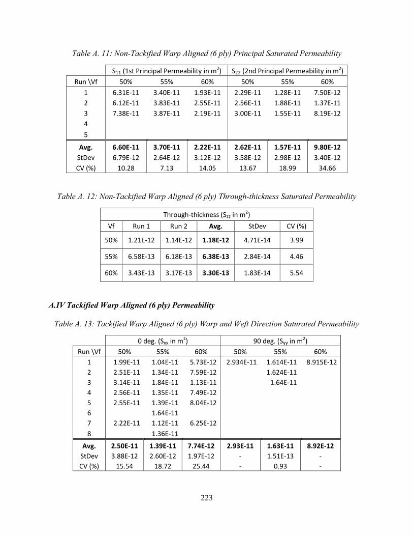
223
Table A. 11: Non-Tackified Warp Aligned (6 ply) Principal Saturated Permeability
S11 (1st Principal Permeability in m2) S22 (2nd Principal Permeability in m2)
Run \Vf 50% 55% 60% 50% 55% 60%
1 6.31E-11 3.40E-11 1.93E-11 2.29E-11 1.28E-11 7.50E-12
2 6.12E-11 3.83E-11 2.55E-11 2.56E-11 1.88E-11 1.37E-11
3 7.38E-11 3.87E-11 2.19E-11 3.00E-11 1.55E-11 8.19E-12
4
5
Avg. 6.60E-11 3.70E-11 2.22E-11 2.62E-11 1.57E-11 9.80E-12
StDev 6.79E-12 2.64E-12 3.12E-12 3.58E-12 2.98E-12 3.40E-12
CV (%) 10.28 7.13 14.05 13.67 18.99 34.66
Table A. 12: Non-Tackified Warp Aligned (6 ply) Through-thickness Saturated Permeability
Through-thickness (Szz in m2)
Vf Run 1 Run 2 Avg. StDev CV (%)
50% 1.21E-12 1.14E-12 1.18E-12 4.71E-14 3.99
55% 6.58E-13 6.18E-13 6.38E-13 2.84E-14 4.46
60% 3.43E-13 3.17E-13 3.30E-13 1.83E-14 5.54
A.IV Tackified Warp Aligned (6 ply) Permeability
Table A. 13: Tackified Warp Aligned (6 ply) Warp and Weft Direction Saturated Permeability
0 deg. (Sxx in m2) 90 deg. (Syy in m2)
Run \Vf 50% 55% 60% 50% 55% 60%
1 1.99E-11 1.04E-11 5.73E-12 2.934E-11 1.614E-11 8.915E-12
2 2.51E-11 1.34E-11 7.59E-12
1.624E-11
3 3.14E-11 1.84E-11 1.13E-11
1.64E-11
4 2.56E-11 1.35E-11 7.49E-12
5 2.55E-11 1.39E-11 8.04E-12
6 1.64E-11
7 2.22E-11 1.12E-11 6.25E-12
8 1.36E-11
Avg. 2.50E-11 1.39E-11 7.74E-12 2.93E-11 1.63E-11 8.92E-12
StDev 3.88E-12 2.60E-12 1.97E-12 - 1.51E-13 -
CV (%) 15.54 18.72 25.44 - 0.93 -
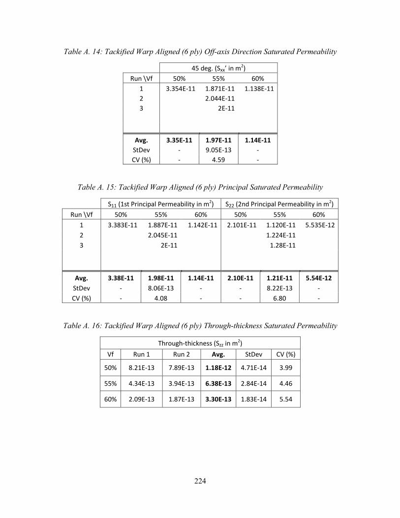
224
Table A. 14: Tackified Warp Aligned (6 ply) Off-axis Direction Saturated Permeability
45 deg. (Sxx’ in m2)
Run \Vf 50% 55% 60%
1 3.354E-11 1.871E-11 1.138E-11
2
2.044E-11
3
2E-11
Avg. 3.35E-11 1.97E-11 1.14E-11
StDev - 9.05E-13 -
CV (%) - 4.59 -
Table A. 15: Tackified Warp Aligned (6 ply) Principal Saturated Permeability
S11 (1st Principal Permeability in m2) S22 (2nd Principal Permeability in m2)
Run \Vf 50% 55% 60% 50% 55% 60%
1 3.383E-11 1.887E-11 1.142E-11 2.101E-11 1.120E-11 5.535E-12
2
2.045E-11
1.224E-11
3
2E-11
1.28E-11
Avg. 3.38E-11 1.98E-11 1.14E-11 2.10E-11 1.21E-11 5.54E-12
StDev - 8.06E-13 - - 8.22E-13 -
CV (%) - 4.08 - - 6.80 -
Table A. 16: Tackified Warp Aligned (6 ply) Through-thickness Saturated Permeability
Through-thickness (Szz in m2)
Vf Run 1 Run 2 Avg. StDev CV (%)
50% 8.21E-13 7.89E-13 1.18E-12 4.71E-14 3.99
55% 4.34E-13 3.94E-13 6.38E-13 2.84E-14 4.46
60% 2.09E-13 1.87E-13 3.30E-13 1.83E-14 5.54
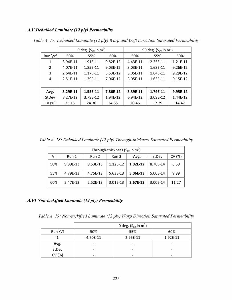
225
A.V Debulked Laminate (12 ply) Permeability
Table A. 17: Debulked Laminate (12 ply) Warp and Weft Direction Saturated Permeability
0 deg. (Sxx in m2) 90 deg. (Syy in m2)
Run \Vf 50% 55% 60% 50% 55% 60%
1 3.94E-11 1.91E-11 9.82E-12 4.43E-11 2.25E-11 1.21E-11
2 4.07E-11 1.85E-11 9.03E-12 3.03E-11 1.63E-11 9.26E-12
3 2.64E-11 1.17E-11 5.53E-12 3.05E-11 1.64E-11 9.29E-12
4 2.51E-11 1.29E-11 7.06E-12 3.05E-11 1.63E-11 9.15E-12
Avg. 3.29E-11 1.55E-11 7.86E-12 3.39E-11 1.79E-11 9.95E-12
StDev 8.27E-12 3.79E-12 1.94E-12 6.94E-12 3.09E-12 1.44E-12
CV (%) 25.15 24.36 24.65 20.46 17.29 14.47
Table A. 18: Debulked Laminate (12 ply) Through-thickness Saturated Permeability
Through-thickness (Szz in m2)
Vf Run 1 Run 2 Run 3 Avg. StDev CV (%)
50% 9.89E-13 9.53E-13 1.12E-12 1.02E-12 8.76E-14 8.59
55% 4.79E-13 4.75E-13 5.63E-13 5.06E-13 5.00E-14 9.89
60% 2.47E-13 2.52E-13 3.01E-13 2.67E-13 3.00E-14 11.27
A.VI Non-tackified Laminate (12 ply) Permeability
Table A. 19: Non-tackified Laminate (12 ply) Warp Direction Saturated Permeability
0 deg. (Sxx in m2)
Run \Vf 50% 55% 60%
1 4.70E-11 2.95E-11 1.92E-11
Avg. - - -
StDev - - -
CV (%) - - -
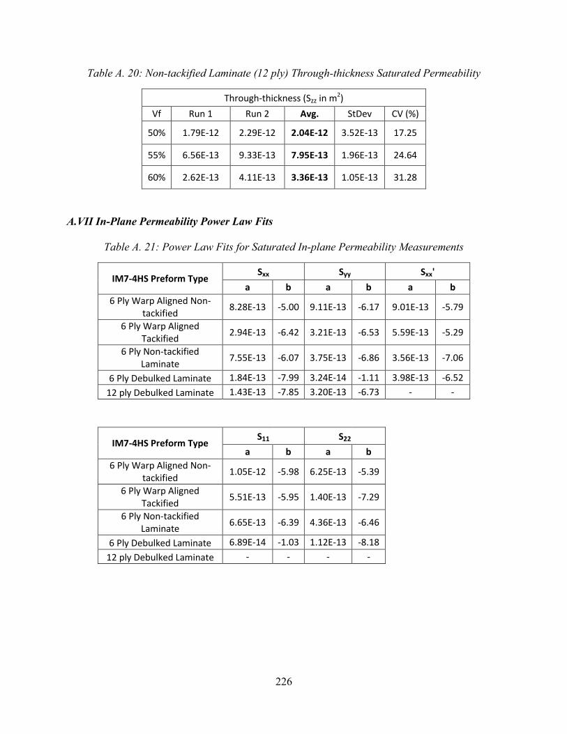
226
Table A. 20: Non-tackified Laminate (12 ply) Through-thickness Saturated Permeability
Through-thickness (Szz in m2)
Vf Run 1 Run 2 Avg. StDev CV (%)
50% 1.79E-12 2.29E-12 2.04E-12 3.52E-13 17.25
55% 6.56E-13 9.33E-13 7.95E-13 1.96E-13 24.64
60% 2.62E-13 4.11E-13 3.36E-13 1.05E-13 31.28
A.VII In-Plane Permeability Power Law Fits
Table A. 21: Power Law Fits for Saturated In-plane Permeability Measurements
IM7-4HS Preform Type Sxx Syy Sxx'
a b a b a b
6 Ply Warp Aligned Non-tackified
8.28E-13 -5.00 9.11E-13 -6.17 9.01E-13 -5.79
6 Ply Warp Aligned Tackified
2.94E-13 -6.42 3.21E-13 -6.53 5.59E-13 -5.29
6 Ply Non-tackified Laminate
7.55E-13 -6.07 3.75E-13 -6.86 3.56E-13 -7.06
6 Ply Debulked Laminate 1.84E-13 -7.99 3.24E-14 -1.11 3.98E-13 -6.52
12 ply Debulked Laminate 1.43E-13 -7.85 3.20E-13 -6.73 - -
IM7-4HS Preform Type S11 S22
a b a b
6 Ply Warp Aligned Non-tackified
1.05E-12 -5.98 6.25E-13 -5.39
6 Ply Warp Aligned Tackified
5.51E-13 -5.95 1.40E-13 -7.29
6 Ply Non-tackified Laminate
6.65E-13 -6.39 4.36E-13 -6.46
6 Ply Debulked Laminate 6.89E-14 -1.03 1.12E-13 -8.18
12 ply Debulked Laminate - - - -
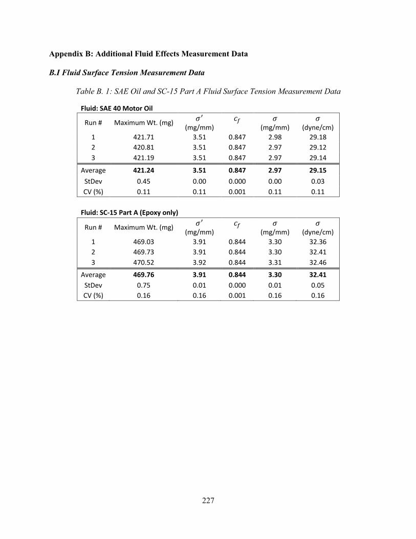
227
Appendix B: Additional Fluid Effects Measurement Data
B.I Fluid Surface Tension Measurement Data
Table B. 1: SAE Oil and SC-15 Part A Fluid Surface Tension Measurement Data
Fluid: SAE 40 Motor Oil
Run # Maximum Wt. (mg) 𝜎′
(mg/mm) 𝑐𝑓 𝜎
(mg/mm) 𝜎
(dyne/cm)
1 421.71 3.51 0.847 2.98 29.18
2 420.81 3.51 0.847 2.97 29.12
3 421.19 3.51 0.847 2.97 29.14
Average 421.24 3.51 0.847 2.97 29.15
StDev 0.45 0.00 0.000 0.00 0.03
CV (%) 0.11 0.11 0.001 0.11 0.11
Fluid: SC-15 Part A (Epoxy only)
Run # Maximum Wt. (mg) 𝜎′
(mg/mm) 𝑐𝑓 𝜎
(mg/mm) 𝜎
(dyne/cm)
1 469.03 3.91 0.844 3.30 32.36
2 469.73 3.91 0.844 3.30 32.41
3 470.52 3.92 0.844 3.31 32.46
Average 469.76 3.91 0.844 3.30 32.41
StDev 0.75 0.01 0.000 0.01 0.05
CV (%) 0.16 0.16 0.001 0.16 0.16

228
B.II Du Noüy Ring Sample Wetting Graphs
Figure B. 1: Wetting Force versus Immersion Depth of Du Noüy Ring in SC-15 Part A
Figure B. 2: Wetting Force versus Immersion Depth of Du Noüy Ring in SAE 40 Oil
-200
-100
0
100
200
300
400
500
0 2 4 6 8 10
We
ttin
g Fo
rce
(m
g)
Immersion Depth (mm)
Wetting Force
-100
0
100
200
300
400
500
0 2 4 6 8 10
We
ttin
g Fo
rce
(m
g)
Immersion Depth (mm)
Wetting Force

229
B.III Fiber Diameter Measurement Data Table B. 2: IM7 Fiber Diameter Data from Laser-scan Micromemeter Measurements
IM7 Fiber Diameter Measurements (µm)
Sample #
Point 1
Point 2
Point 3
Sample Avg.
Sample StDev
Among 3 Pts.
CV (%) Among 3
Pts.
Perimeter (from Avg.)
1 5.22 5.27 5.38 5.29 0.08 1.55 16.62
2 5.22 5.25 5.2 5.22 0.03 0.48 16.41
3 8.35 7.98 7.82 8.05 0.27 3.38 25.29
4 5.63 5.73 5.71 5.69 0.05 0.93 17.88
5 6.21 5.52 5.6 5.78 0.38 6.53 18.15
6 5.44 5.38 5.65 5.49 0.14 2.58 17.25
7 5.35 5.44 5.29 5.36 0.08 1.41 16.84
8 5.68 5.61 6.8 6.03 0.67 11.07 18.94
9 5.64 5.58 5.58 5.60 0.03 0.62 17.59
10 5.51 5.75 5.69 5.65 0.12 2.21 17.75
11 5.59 5.47 5.38 5.48 0.11 1.92 17.22
12 5.69 6.63 6.71 6.34 0.57 8.94 19.93
13 5.8 5.7 5.94 5.81 0.12 2.07 18.26
14 5.51 5.44 5.41 5.45 0.05 0.94 17.13
15 5.59 5.5 5.41 5.50 0.09 1.64 17.28
16 5.22 5.15 5.19 5.19 0.04 0.68 16.29
17 5.38 5.49 5.39 5.42 0.06 1.12 17.03
18 5.54 5.59 5.77 5.63 0.12 2.15 17.70
19 5.55 5.58 5.58 5.57 0.02 0.31 17.50
20 5.5 5.65 5.6 5.58 0.08 1.37 17.54
21 5.35 5.37 5.4 5.37 0.03 0.47 16.88
22 5.51 6.14 5.34 5.66 0.42 7.44 17.79
23 5.92 5.89 5.92 5.91 0.02 0.29 18.57
24 5.4 5.35 5.45 5.40 0.05 0.93 16.96
25 5.38 5.32 5.3 5.33 0.04 0.78 16.76
26 5.65 5.64 5.67 5.65 0.02 0.27 17.76
27 6.06 5.94 6.07 6.02 0.07 1.20 18.92
28 5.72 5.66 5.83 5.74 0.09 1.50 18.02
29 5.19 5.24 5.23 5.22 0.03 0.51 16.40
Average 5.65 5.66 5.70 5.67 0.13 2.25 17.82
Average without
#3 5.55 5.58 5.62 5.59 0.13 2.21 17.55

230
B.IV Micro-Wilhelmy Sample Status List
Table B. 3: Micro-Wilhelmy Sample Usage Statuses
Sample ID
Test Fluid Advancing
Data Receding
Data
Fiber-1 SAE 40 Oil Used Used
Fiber-2 SAE 40 Oil Used Used
Fiber-3 SAE 40 Oil Unused Unused
Fiber-4 SAE 40 Oil Used Used
Fiber-5 SAE 40 Oil Used Used
Fiber-6 SAE 40 Oil Used Used
Fiber-7 SAE 40 Oil Used Used
Fiber-8 SAE 40 Oil Unused Unused
Fiber-9 SAE 40 Oil Unused Unused
Fiber-10 SAE 40 Oil Used Unused
Fiber-11 SAE 40 Oil Used Used
Fiber-12 SAE 40 Oil Used Used
Fiber-13 SAE 40 Oil Used Used
Fiber-14 SC-15 Unused Unused
Fiber-15 SC-15 Unused Unused
Fiber-16 SC-15 Unused Unused
Fiber-17 SC-15 Unused Unused
Fiber-18 SC-15 Unused Unused
Fiber-19 SC-15 Unused Unused
Fiber-20 SC-15 Unused Unused
Fiber-21 SC-15 Unused Unused
Fiber-22 SC-15 Part A only Used Used
Fiber-23 SC-15 Part A only Used Used
Fiber-24 SC-15 Part A only Used Used
Fiber-25 SC-15 Part A only Used Used
Fiber-26 SC-15 Part A only Used Used
Fiber-27 SC-15 Part A only Used Used
Fiber-28 SC-15 Part A only Used Used
Fiber-29 SC-15 Part A only Used Unused
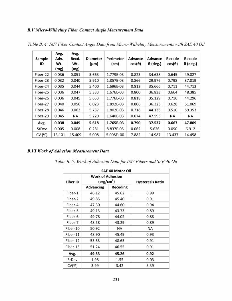
231
B.V Micro-Wilhelmy Fiber Contact Angle Measurement Data
Table B. 4: IM7 Fiber Contact Angle Data from Micro-Wilhelmy Measurements with SAE 40 Oil
Sample ID
Avg. Adv. Wt. (mg)
Avg. Recd. Wt. (mg)
Diameter (μm)
Perimeter (cm)
Advance cos(θ)
Advance θ (deg.)
Recede cos(θ)
Recede θ (deg.)
Fiber-22 0.036 0.051 5.663 1.779E-03 0.823 34.638 0.645 49.827
Fiber-23 0.032 0.040 5.910 1.857E-03 0.866 29.976 0.798 37.019
Fiber-24 0.035 0.044 5.400 1.696E-03 0.812 35.666 0.711 44.713
Fiber-25 0.036 0.047 5.333 1.676E-03 0.800 36.833 0.664 48.385
Fiber-26 0.036 0.045 5.653 1.776E-03 0.818 35.129 0.716 44.296
Fiber-27 0.040 0.056 6.023 1.892E-03 0.806 36.323 0.628 51.069
Fiber-28 0.046 0.062 5.737 1.802E-03 0.718 44.136 0.510 59.353
Fiber-29 0.045 NA 5.220 1.640E-03 0.674 47.595 NA NA
Avg. 0.038 0.049 5.618 1.765E-03 0.790 37.537 0.667 47.809
StDev 0.005 0.008 0.281 8.837E-05 0.062 5.626 0.090 6.912
CV (%) 13.101 15.409 5.008 5.008E+00 7.882 14.987 13.437 14.458
B.VI Work of Adhesion Measurement Data
Table B. 5: Work of Adhesion Data for IM7 Fibers and SAE 40 Oil
SAE 40 Motor Oil
Fiber ID
Work of Adhesion (erg/cm2) Hysteresis Ratio
Advancing Receding
Fiber-1 46.12 45.62 0.99
Fiber-2 49.85 45.40 0.91
Fiber-4 47.30 44.60 0.94
Fiber-5 49.13 43.73 0.89
Fiber-6 49.78 44.02 0.88
Fiber-7 48.58 43.29 0.89
Fiber-10 50.92 NA NA
Fiber-11 48.90 45.49 0.93
Fiber-12 53.53 48.65 0.91
Fiber-13 51.24 46.55 0.91
Avg. 49.53 45.26 0.92
StDev 1.98 1.55 0.03
CV(%) 3.99 3.42 3.39

232
Table B. 6: Work of Adhesion Data for IM7 Fibers and SC-15 Part A
SC-15 Epoxy (Part A only)
Fiber ID
Work of Adhesion (erg/cm2) Hysteresis Ratio
Advancing Receding
Fiber-22 59.07 53.32 0.90
Fiber-23 60.48 58.29 0.96
Fiber-24 58.74 55.44 0.94
Fiber-25 58.35 53.93 0.92
Fiber-26 58.92 55.61 0.94
Fiber-27 58.52 52.77 0.90
Fiber-28 55.67 48.93 0.88
Fiber-29 54.27 NA NA
Avg. 58.00 54.04 0.92
StDev 1.89 2.69 0.03
CV(%) 3.25 4.98 2.99

233
Appendix C: MATLAB Scripts
C.I Principal Permeability Calculator %Principal Permeability Calculator %Stephen Sommerlot 3/29/13 %CVRC %Code takes input from in-plane permeability testing data to find principal %permeabilities S11 and S22 and direction. Uses Mohr type transformation %~~~~~~~~~~~~~~~~~~~~~~~~~~~~~~~~~~~~~~~~~~~~~~~~~~~~~~~~~~~~~~
%clears the workspace clear all
%prompts user for permeability data input Sxx = input('Enter Sxx permeability value: '); Syy = input('Enter Syy permeability value: '); Sxx_prime = input('Enter Sxx_prime permeability value (45 deg): ');
%computes off-axis permeability tensor component Sxy = Sxx_prime - (.5*Sxx) - (.5*Syy)
%disaplys 2-D permeability tensor S_bar = [Sxx, Sxy; Sxy, Syy]
%rotates S_bar to get S'_bar deg = pi/4; % 45 deg %deg = 0.523598776; % for 30 deg. a_bar_T = [cos(deg), sin(deg); -sin(deg), cos(deg)]; a_bar = [cos(deg), -sin(deg); sin(deg), cos(deg)];
S_prime_bar = a_bar_T * S_bar * a_bar;
%finds principal permeabilities prinicpal_permeabilities = eig(S_prime_bar)
S11 = max(prinicpal_permeabilities) S22 = min(prinicpal_permeabilities)
%finds principal direction vector [V,D] = eig(S_prime_bar)
%calculates angle of rotation (degrees), this is a very sensitive calculation
to %experimental scatter beta_from_S_bar = (atan(2*S_bar(1,2)/(S_bar(1,1)-S_bar(2,2)))*180/pi)/2

234
C.II Image Processing Script for Radial Infusions % Stephen Sommerlot % CVRC % 3/5/14 % Script for ellipse detection in radial-visual fabric flow fronts % Uses ellipse calculations for unsaturated permeability determination % based on paper: radial flow permeability measurement. Part A and B by % Weitzenboeck % Note: constant pressure injection formulation
% Prompt to get test data from user material = input('Enter Material Name: ', 's'); %'Non-Tackified IM7-4HS' OR
Tackified IM7-4HS ply_num = 14; %input('Enter Ply Number: '); Vf_in = 50; % input('Enter Material Vf(%): '); Vf = Vf_in/100; porosity = 1- Vf; inlet_diameter = 3/8; % = input('Enter Punch Diameter (in.) Used for Inlet
(can be a fraction): '); inlet_rad_m = (inlet_diameter*.0254)/2; x0 = inlet_rad_m; y0 = inlet_rad_m; t0 = 0; %27; % = input('Enter Initial Starting Time(s) Seen on Stopwatch
for Flow Propagation: '); % 27s for SS2 % t_cutoff = input('Enter Cutoff Time of Time for Pressure Data: '); % 1200s
for SS2
% Read test pressures from file, get average and StDev of inlet pressure cd('C:\Users\sommerl4\Documents\MATLAB\Edge
Detect\coderdemo_edge_detection\Radial_Perm_Data')
psig_in_file = load('Pressure_Inlet_0-6PSIG_tack2.txt'); psig_in_full = psig_in_file(:,2); time_in_full = psig_in_file(:,1); % Uncomment for manual truncation % time_diff = abs(time_in_full - t0); % [idx idx] = min(time_diff); % closest_time_to_t0 = time_in_full(idx); % time_diff2 =abs(time_in_full - t_cutoff); % [idx2 idx2] = min(time_diff2); % time_in = time_in_full(idx:idx2); % psi_in = psig_in_full(idx:idx2); avg_psi_in = mean(psig_in_full); Pressure_StDev_psi = std(psig_in_full); kpa_in = 6.89475729*psig_in_full; avg_kpa_in = mean(kpa_in); avg_pa_in = avg_kpa_in*1000; Pressure_StDev = std(kpa_in); pressure_CV = Pressure_StDev*100/avg_kpa_in;
cd('C:\Users\sommerl4\Documents\MATLAB\Edge
Detect\coderdemo_edge_detection\Radial_Perm_Data')
% load image

235
image = imread('IM7_tack_run2_3-7-14_10min.png'); imshow(image)
% gives user points to outline ellipse (10 in each quadrant) [x,y] = ginput(40);
imshow(image) hold on plot(x,y, '+') h = gca; % get current axis handle
% call ellipse finding function % outputs structure of ellipse props ellipse_t = fit_ellipse(x,y,h)
% break structure into numerics using ellipse function defs ellipse_cell = struct2cell(ellipse_t); a = cell2mat(ellipse_cell(1)); % sub axis (radius) of the X axis of the non-
tilt ellipse b = cell2mat(ellipse_cell(2)) ; % sub axis (radius) of the Y axis of the non-
tilt ellipse phi = cell2mat(ellipse_cell(3)); % orientation in radians of the ellipse
(tilt) X0 = cell2mat(ellipse_cell(4)); % center at the X axis of the non-tilt
ellipse Y0 = cell2mat(ellipse_cell(5)); % center at the Y axis of the non-tilt
ellipse X0_in = cell2mat(ellipse_cell(6)); % center at the X axis of the tilted
ellipse Y0_in = cell2mat(ellipse_cell(7)); % center at the Y axis of the tilted
ellipse long_axis = cell2mat(ellipse_cell(8)); % size of the long axis of the
ellipse short_axis = cell2mat(ellipse_cell(9)); % size of the short axis of the
ellipse
% beta angle (just phi converted to degrees) beta = phi*(180/pi);
%for 45 deg. radius based on non-tilted ellipse (radius should be same just %not rotated) deg45 = pi/4; x45 = a*cos(deg45); y45 = b*sin(deg45); r45 = sqrt(x45^2 + y45^2);
% get reference measurement imtool(image) distance = 9.1160e+01; %input('Enter Reference Distance Pixel Length: ');
uncomment this to user define distance refdist = distance;
t_min_current = input('Enter Current Stopwatch Minutes on Image: '); t_sec_current = input('Enter Current Stopwatch Seconds on Image: '); t = ((t_min_current)*60 + t_sec_current) - t0;
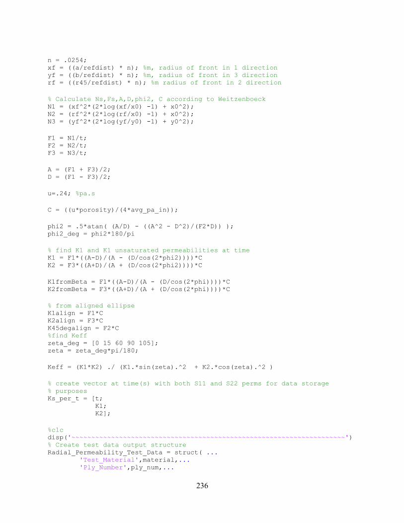
236
n = .0254; xf = ((a/refdist) * n); %m, radius of front in 1 direction yf = ((b/refdist) * n); %m, radius of front in 3 direction rf = ((r45/refdist) * n); %m radius of front in 2 direction
% Calculate Ns,Fs,A,D,phi2, C according to Weitzenboeck N1 = (xf^2*(2*log(xf/x0) -1) + x0^2); N2 = (rf^2*(2*log(rf/x0) -1) + x0^2); N3 = (yf^2*(2*log(yf/y0) -1) + y0^2);
F1 = N1/t; F2 = N2/t; F3 = N3/t;
A = (F1 + F3)/2; D = (F1 - F3)/2;
u=.24; %pa.s
C = ((u*porosity)/(4*avg_pa_in));
phi2 = .5*atan( (A/D) - ((A^2 - D^2)/(F2*D)) ); phi2_deg = phi2*180/pi
% find K1 and K1 unsaturated permeabilities at time K1 = F1*((A-D)/(A - (D/cos(2*phi2))))*C K2 = F3*((A+D)/(A + (D/cos(2*phi2))))*C
K1fromBeta = F1*((A-D)/(A - (D/cos(2*phi))))*C K2fromBeta = F3*((A+D)/(A + (D/cos(2*phi))))*C
% from aligned ellipse K1align = F1*C K2align = F3*C K45degalign = F2*C %find Keff zeta_deg = [0 15 60 90 105]; zeta = zeta_deg*pi/180;
Keff = (K1*K2) ./ (K1.*sin(zeta).^2 + K2.*cos(zeta).^2 )
% create vector at time(s) with both S11 and S22 perms for data storage % purposes Ks_per_t = [t; K1; K2];
%clc disp('~~~~~~~~~~~~~~~~~~~~~~~~~~~~~~~~~~~~~~~~~~~~~~~~~~~~~~~~~~~~~~~~~~~~~') % Create test data output structure Radial_Permeability_Test_Data = struct( ... 'Test_Material',material,... 'Ply_Number',ply_num,...

237
'Fiber_Volume_Fraction_Vf',Vf,... 'Preform_Inlet_Diameter_in',inlet_diameter,... 'Average_Inlet_Pressure_psi',avg_psi_in,... 'Standard_Deviation_of_Inlet_Pressure_psi',Pressure_StDev_psi,... 'Fluid_Viscosity_Pa_s',u,... 'Beta_Angle',beta,... 'K1', K1, ... 'K2', K2, ... 'Time_at_Measurement_s', t)

238
REFERENCES

239
REFERENCES
[1] J. Hale, “Boeing 787 from the Ground Up,” AERO, no. QTR_04 2006, pp. 17–23.
[2] G. Marsh, “Composites get in deep with new-generation engine,” Reinf. Plast., vol. 50, no. 11, pp. 26–29, Dec. 2006.
[3] C. Soutis, “Carbon fiber reinforced plastics in aircraft construction,” Mater. Sci. Eng. A, vol. 412, no. 1–2, pp. 171–176, Dec. 2005.
[4] M. W. Hyer, Stress Analysis of Fiber-Reinforced Composite Materials, Updated Edition. Lancaster, PA: DEStech Publications, Inc., 2009.
[5] C.-L. Lee and K.-H. Wei, “Effect of material and process variables on the performance of resin-transfer-molded epoxy fabric composites,” J. Appl. Polym. Sci., vol. 77, no. 10, pp. 2149–2155, 2000.
[6] S. Abrate, “Resin flow in fiber preforms,” Appl. Mech. Rev., vol. 55, no. 6, pp. 579–599, Oct. 2002.
[7] P. Hubert and A. Poursartip, “A Review of Flow and Compaction Modelling Relevant to Thermoset Matrix Laminate Processing,” J. Reinf. Plast. Compos., vol. 17, no. 4, pp. 286–318, Mar. 1998.
[8] V. Rohatgi, L. J. Lee, and A. Melton, “Overview of fibre preforming,” in Resin Transfer Moulding for Aerospace Structures, T. M. Kruckenberg and R. Paton, Eds. Springer Netherlands, 1998, pp. 148–176.
[9] V. Rohatgi and L. J. Lee, “Moldability of Tackified Fiber Preforms in Liquid Composite Molding,” J. Compos. Mater., vol. 31, no. 7, pp. 720–744, Apr. 1997.
[10] C.-H. Shih and L. J. Lee, “Tackification of Textile Fiber Preforms in Resin Transfer Molding,” J. Compos. Mater., vol. 35, no. 21, pp. 1954–1981, Nov. 2001.
[11] G. Estrada, C. Vieux-Pernon, and S. G. Advani, “Experimental Characterization of the Influence of Tackifier Material on Preform Permeability,” J. Compos. Mater., vol. 36, no. 19, pp. 2297–2310, Oct. 2002.
[12] J. Chen, D. Backes, and K. Jayaraman, “Dynamics of binder displacement in liquid molding,” Polym. Compos., vol. 17, no. 1, pp. 23–33, Feb. 1996.
[13] L. Aktas, D. P. Bauman, S. T. Bowen, M. C. Saha, and M. C. Altan, “Effect of Distribution Media Length and Multiwalled Carbon Nanotubes on the Formation of Voids in VARTM Composites,” J. Eng. Mater. Technol., vol. 133, no. 4, pp. 041006–041006, Oct. 2011.
240
[14] F. F. Luz, S. C. Amico, J. Á. Souza, E. S. Barbosa, and A. G. B. de Lima, “Resin Transfer Molding Process: Fundamentals, Numerical Computation and Experiments,” in Numerical Analysis of Heat and Mass Transfer in Porous Media, J. M. P. Q. Delgado, A. G. B. de Lima, and M. V. da Silva, Eds. Springer Berlin Heidelberg, 2012, pp. 121–151.
[15] K. Han, S. Jiang, C. Zhang, and B. Wang, “Flow modeling and simulation of SCRIMP for composites manufacturing,” Compos. Part Appl. Sci. Manuf., vol. 31, no. 1, pp. 79–86, Jan. 2000.
[16] P. Ermanni, C. Di Fratta, F. Trochu, and L. Nicolais, “Molding: Liquid Composite Molding (LCM),” in Wiley Encyclopedia of Composites, John Wiley & Sons, Inc., 2011.
[17] S. G. Advani and E. M. Sozer, Process Modeling in Composites Manufacturing, Second Edition. CRC Press, 2012.
[18] G. Morren, M. Bottiglieri, S. Bossuyt, H. Sol, D. Lecompte, B. Verleye, and S. V. Lomov, “A reference specimen for permeability measurements of fibrous reinforcements for RTM,” Compos. Part Appl. Sci. Manuf., vol. 40, no. 3, pp. 244–250, Mar. 2009.
[19] C. Lai and W. Young, “The effects of preforming induced variable permeabilities on the rtm molding flow,” Polym. Compos., vol. 20, no. 2, pp. 225–239, 1999.
[20] V. Michaud and L. Nicolais, “Fibrous Preforms and Preforming,” in Wiley Encyclopedia of Composites, John Wiley & Sons, Inc., 2011.
[21] J. C. Brody and J. W. Gillespie, “Reactive and non-reactive binders in glass/vinyl ester composites,” Polym. Compos., vol. 26, no. 3, pp. 377–387, Jun. 2005.
[22] S. Aranda, F. Klunker, and G. Ziegmann, “Influence of the Binding System on the Compaction Behaviour of NCF Carbon Fibre Reinforcements,” 18th Int. Conf. Compos. Mater., Aug. 2011.
[23] M. Tanoglu, S. Robert, D. Heider, S. H. McKnight, V. Brachos, and J. W. Gillespie Jr., “Effects of thermoplastic preforming binder on the properties of S2-glass fabric reinforced epoxy composites,” Int. J. Adhes. Adhes., vol. 21, no. 3, pp. 187–195, 2001.
[24] M. Tanoğlu and A. Tuğrul Seyhan, “Investigating the effects of a polyester preforming binder on the mechanical and ballistic performance of E-glass fiber reinforced polyester composites,” Int. J. Adhes. Adhes., vol. 23, no. 1, pp. 1–8, 2003.
[25] J. Li, C. Zhang, R. Liang, and B. Wang, “Statistical characterization and robust design of RTM processes,” Compos. Part Appl. Sci. Manuf., vol. 36, no. 5, pp. 564–580, May 2005.
[26] S. J. Sommerlot, T. J. Luchini, and A. C. Loos, “Modeling Advancing Flow Fronts in Composite Manufacturing,” in Proceedings of the American Society for Composites 29th Technical Conference, San Diego, CA, September 8-10.

241
[27] C. H. Park and L. Woo, “Modeling void formation and unsaturated flow in liquid composite molding processes: a survey and review,” J. Reinf. Plast. Compos., vol. 30, no. 11, pp. 957–977, Jun. 2011.
[28] K.-T. Hsiao, R. Little, O. Restrepo, and B. Minaie, “A study of direct cure kinetics characterization during liquid composite molding,” Compos. Part Appl. Sci. Manuf., vol. 37, no. 6, pp. 925–933, Jun. 2006.
[29] A. Shojaei, S. R. Ghaffarian, and S. M. H. Karimian, “Modeling and simulation approaches in the resin transfer molding process: A review,” Polym. Compos., vol. 24, no. 4, pp. 525–544, 2003.
[30] H. Abdellaoui and J. Echaabi, “Rheological models for modeling the viscoelastic behavior in liquid composite molding processes (LCM) review,” J. Reinf. Plast. Compos., vol. 33, no. 8, pp. 714–732, Apr. 2014.
[31] B. Chen, A. H.-D. Cheng, and T.-W. Chou, “A nonlinear compaction model for fibrous preforms,” Compos. Part Appl. Sci. Manuf., vol. 32, no. 5, pp. 701–707, May 2001.
[32] M. Matsudaira and H. Qin, “Features and Mechanical Parameters of a Fabric’s Compressional Property,” J. Text. Inst., vol. 86, no. 3, pp. 476–486, Jan. 1995.
[33] B. Chen, E. J. Lang, and T.-W. Chou, “Experimental and theoretical studies of fabric compaction behavior in resin transfer molding,” Mater. Sci. Eng. A, vol. 317, no. 1–2, pp. 188–196, Oct. 2001.
[34] V. Michaud and A. Mortensen, “Infiltration processing of fibre reinforced composites: governing phenomena,” Compos. Part Appl. Sci. Manuf., vol. 32, no. 8, pp. 981–996, Aug. 2001.
[35] M. Li, Y. Gu, Z. Zhang, and Z. Sun, “A simple method for the measurement of compaction and corresponding transverse permeability of composite prepregs,” Polym. Compos., vol. 28, no. 1, pp. 61–70, Feb. 2007.
[36] B. W. Grimsley, “Characterization of the Vacuum Assisted Resin Transfer Molding Process for Fabrication of Aerospace Composites,” Virginia Polytechnic Institute and State University, Blacksburg, VA, 2005.
[37] B. W. Grimsley, R. J. Cano, P. Hubert, A. C. Loos, C. B. Kellen, and B. J. Jensen, “Preform Characterization in VARTM Process Model Development,” presented at the 36th International SAMPE Technical Conference, San Diego, CA, 2004.
[38] A. A. Somashekar, S. Bickerton, and D. Bhattacharyya, “An experimental investigation of non-elastic deformation of fibrous reinforcements in composites manufacturing,” Compos. Part Appl. Sci. Manuf., vol. 37, no. 6, pp. 858–867, Jun. 2006.

242
[39] Y. R. Kim, S. P. McCarthy, and J. P. Fanucci, “Compressibility and relaxation of fiber reinforcements during composite processing,” Polym. Compos., vol. 12, no. 1, pp. 13–19, 1991.
[40] C. M. van Wyk, “20—Note on the Compressibility of Wool,” J. Text. Inst. Trans., vol. 37, no. 12, pp. T285–T292, Dec. 1946.
[41] G. L. Batch, S. Cumiskey, and C. W. Macosko, “Compaction of fiber reinforcements,” Polym. Compos., vol. 23, no. 3, pp. 307–318, 2002.
[42] A. C. Loos and J. D. MacRae, “A process simulation model for the manufacture of a blade-stiffened panel by the resin film infusion process,” Compos. Sci. Technol., vol. 56, no. 3, pp. 273–289, 1996.
[43] V. H. Hammond, A. C. Loos, H. B. Dexter, and G. Hasko, “Verification of a two-dimensional infiltration model for the resin transfer molding process,” Virginia Polytechnic Institute and State University, Blacksburg, VA, CCMS‑93‑15, VPI‑E‑93‑09, Aug. 1993.
[44] G. Tuncol, “Modeling the Vacuum Assisted Resin Transfer Molding (VARTM) Process for Fabrication of Fiber/Metal Hybrid Laminates,” Michigan State University, East Lansing, MI, 2010.
[45] J. C. Fingerson, A. C. Loos, and H. B. Dexter, “Verification of a Three-Dimensional Resin Transfer Molding Process Simulation Model,” Virginia Polytechnic Institute and State University, Blacksburg, VA, CCMS-95-10, VPI-E-95-04, Sep. 1995.
[46] F. Robitaille and R. Gauvin, “Compaction of textile reinforcements for composites manufacturing. I: Review of experimental results,” Polym. Compos., vol. 19, no. 2, pp. 198–216, 1998.
[47] V. J. Michaud, A. Mortensen, and J. L. Sommer, “Infiltration of fibrous preforms by a pure metal: Part V. Influence of preform compressibility,” Metall. Mater. Trans. A, vol. 30, no. 2, pp. 471–482, Feb. 1999.
[48] P. Boisse, Composite Reinforcements for Optimum Performance. Elsevier, 2011.
[49] S. Bickerton, S. Comas-Cardona, I. Razali, M. Deléglise, W. A. Walbran, C. Binétruy, and P. Krawczak, “Spatial Compaction and Saturated Permeability Variations of Fibre Reinforcements,” presented at the 9th International Conference on Flow Processes in Composite Materials, Montréal, Canada, 2008.
[50] Z. Cai and T. Gutowski, “The 3-D Deformation Behavior of a Lubricated Fiber Bundle,” J. Compos. Mater., vol. 26, no. 8, pp. 1207–1237, Aug. 1992.
[51] S. Toll, “Packing mechanics of fiber reinforcements,” Polym. Eng. Sci., vol. 38, no. 8, pp. 1337–1350, 1998.
243
[52] S. Toll and J.-A. E. Manson, “Elastic Compression of a Fiber Network,” J. Appl. Mech., vol. 62, no. 1, pp. 223–226, Mar. 1995.
[53] B. Chen and T.-W. Chou, “Compaction of woven-fabric preforms in liquid composite molding processes: single-layer deformation,” Compos. Sci. Technol., vol. 59, no. 10, pp. 1519–1526, Aug. 1999.
[54] B. Chen and T.-W. Chou, “Compaction of woven-fabric preforms: nesting and multi-layer deformation,” Compos. Sci. Technol., vol. 60, no. 12–13, pp. 2223–2231, Sep. 2000.
[55] I. Verpoest and S. V. Lomov, “Virtual textile composites software WiseTex: Integration with micro-mechanical, permeability and structural analysis,” Compos. Sci. Technol., vol. 65, no. 15–16, pp. 2563–2574, Dec. 2005.
[56] H. Lin, M. Sherburn, J. Crookston, A. C. Long, M. J. Clifford, and I. A. Jones, “Finite element modelling of fabric compression,” Model. Simul. Mater. Sci. Eng., vol. 16, no. 3, p. 035010, Apr. 2008.
[57] Q. T. Nguyen, E. Vidal-Sallé, P. Boisse, C. H. Park, A. Saouab, J. Bréard, and G. Hivet, “Mesoscopic scale analyses of textile composite reinforcement compaction,” Compos. Part B Eng., vol. 44, no. 1, pp. 231–241, Jan. 2013.
[58] G. Hivet and P. Boisse, “Consistent 3D geometrical model of fabric elementary cell. Application to a meshing preprocessor for 3D finite element analysis,” Finite Elem. Anal. Des., vol. 42, no. 1, pp. 25–49, 2005.
[59] H. Darcy, Les fontaines publiques de la ville de Dijon: exposition et application ... Victor Dalmont, 1856.
[60] N. K. Naik, M. Sirisha, and A. Inani, “Permeability characterization of polymer matrix composites by RTM/VARTM,” Prog. Aerosp. Sci., vol. 65, pp. 22–40, Feb. 2014.
[61] J. R. Weitzenböck, R. A. Shenoi, and P. A. Wilson, “Measurement of principal permeability with the channel flow experiment,” Polym. Compos., vol. 20, no. 2, pp. 321–335, Apr. 1999.
[62] R. S. Parnas, A. J. Salem, T. A. K. Sadiq, H.-P. Wang, and S. G. Advani, “The interaction between micro- and macro-scopic flow in RTM preforms,” Compos. Struct., vol. 27, no. 1–2, pp. 93–107, 1994.
[63] R. Gauvin, A. Kerachni, and B. Fisa, “Variation of Mat Surface Density and Its Effect on Permeability Evaluation for RTM Modelling,” J. Reinf. Plast. Compos., vol. 13, no. 4, pp. 371–383, Apr. 1994.
[64] S. Drapier, A. Pagot, A. Vautrin, and P. Henrat, “Influence of the stitching density on the transverse permeability of non-crimped new concept (NC2) multiaxial reinforcements: measurements and predictions,” Compos. Sci. Technol., vol. 62, no. 15, pp. 1979–1991, Nov. 2002.

244
[65] A. Shojaei, F. Trochu, S. R. Ghaffarian, S. M. H. Karimian, and L. Lessard, “An Experimental Study of Saturated and Unsaturated Permeabilities in Resin Transfer Molding Based on Unidirectional Flow Measurements,” J. Reinf. Plast. Compos., vol. 23, no. 14, pp. 1515–1536, Sep. 2004.
[66] R. Arbter, J. M. Beraud, C. Binetruy, L. Bizet, J. Bréard, S. Comas-Cardona, C. Demaria, A. Endruweit, P. Ermanni, F. Gommer, S. Hasanovic, P. Henrat, F. Klunker, B. Laine, S. Lavanchy, S. V. Lomov, A. Long, V. Michaud, G. Morren, E. Ruiz, H. Sol, F. Trochu, B. Verleye, M. Wietgrefe, W. Wu, and G. Ziegmann, “Experimental determination of the permeability of textiles: A benchmark exercise,” Compos. Part Appl. Sci. Manuf., vol. 42, no. 9, pp. 1157–1168, Sep. 2011.
[67] T. S. Lundström, R. Stenberg, R. Bergström, H. Partanen, and P. A. Birkeland, “In-plane permeability measurements: a nordic round-robin study,” Compos. Part Appl. Sci. Manuf., vol. 31, no. 1, pp. 29–43, Jan. 2000.
[68] J. B. Alms, N. Correia, S. G. Advani, and E. Ruiz, “Experimental Procedures to Run Longitudinal Injections to Measure Unsaturated Permeability of LCM Reinforcements,” 2010.
[69] N. Vernet, E. Ruiz, S. Advani, J. B. Alms, M. Aubert, M. Barburski, B. Barari, J. M. Beraud, D. C. Berg, N. Correia, M. Danzi, T. Delavière, M. Dickert, C. Di Fratta, A. Endruweit, P. Ermanni, G. Francucci, J. A. Garcia, A. George, C. Hahn, F. Klunker, S. V. Lomov, A. Long, B. Louis, J. Maldonado, R. Meier, V. Michaud, H. Perrin, K. Pillai, E. Rodriguez, F. Trochu, S. Verheyden, M. Wietgrefe, W. Xiong, S. Zaremba, and G. Ziegmann, “Experimental determination of the permeability of engineering textiles: Benchmark II,” Compos. Part Appl. Sci. Manuf., vol. 61, pp. 172–184, Jun. 2014.
[70] R. S. Parnas, K. M. Flynn, and M. E. Dal-Favero, “A permeability database for composites manufacturing,” Polym. Compos., vol. 18, no. 5, pp. 623–633, Oct. 1997.
[71] R. S. Parnas, J. G. Howard, T. L. Luce, and S. G. Advani, “Permeability characterization. Part 1: A proposed standard reference fabric for permeability,” Polym. Compos., vol. 16, no. 6, pp. 429–445, 1995.
[72] K. Okonkwo, P. Simacek, S. G. Advani, and R. S. Parnas, “Characterization of 3D fiber preform permeability tensor in radial flow using an inverse algorithm based on sensors and simulation,” Compos. Part Appl. Sci. Manuf., vol. 42, no. 10, pp. 1283–1292, Oct. 2011.
[73] D. L. Woerdeman, F. R. Phelan, and R. S. Parnas, “Interpretation of 3-D permeability measurements for RTM modeling,” Polym. Compos., vol. 16, no. 6, pp. 470–480, 1995.
[74] J. R. Weitzenböck, R. A. Shenoi, and P. A. Wilson, “Measurement of three-dimensional permeability,” Compos. Part Appl. Sci. Manuf., vol. 29, no. 1–2, pp. 159–169, 1998.
[75] S. H. Ahn, W. I. Lee, and G. S. Springer, “Measurement of the Three-Dimensional Permeability of Fiber Preforms Using Embedded Fiber Optic Sensors,” J. Compos. Mater., vol. 29, no. 6, pp. 714–733, Apr. 1995.

245
[76] P. B. Nedanov and S. G. Advani, “A Method to Determine 3D Permeability of Fibrous Reinforcements,” J. Compos. Mater., vol. 36, no. 2, pp. 241–254, Jan. 2002.
[77] F. LeBel, “Experimental Characterization by Fluorescence of Capillary Flows in the Fiber Tows of Engineering Fabrics,” Open J. Inorg. Non-Met. Mater., vol. 02, no. 03, pp. 25–45, 2012.
[78] G. L. Batch, Y.-T. Chen, and C. W. Macoskot, “Capillary Impregnation of Aligned Fibrous Beds: Experiments and Model,” J. Reinf. Plast. Compos., vol. 15, no. 10, pp. 1027–1051, Oct. 1996.
[79] S. C. Amico and C. Lekakou, “Axial impregnation of a fiber bundle. Part 1: Capillary experiments,” Polym. Compos., vol. 23, no. 2, pp. 249–263, 2002.
[80] K. Hoes, D. Dinescu, H. Sol, M. Vanheule, R. S. Parnas, Y. Luo, and I. Verpoest, “New set-up for measurement of permeability properties of fibrous reinforcements for RTM,” Compos. Part Appl. Sci. Manuf., vol. 33, no. 7, pp. 959–969, Jul. 2002.
[81] J. R. Weitzenböck, R. A. Shenoi, and P. A. Wilson, “Radial flow permeability measurement. Part B: Application,” Compos. Part Appl. Sci. Manuf., vol. 30, no. 6, pp. 797–813, Jun. 1999.
[82] Y. R. Kim, S. P. McCarthy, J. P. Fanucci, S. C. Nolet, and C. KOPPERNAES, “Resin flow through fiber reinforcements during composite processing,” SAMPE Q., vol. 22, no. 3, pp. 16–22, 1991.
[83] G. Lebrun, C. D. Rudd, and R. Gauvin, “Laminate Temperature Distributions and Filling Tine Prediction during Non-Isothermal Impregnation of Fibre Preforms,” J. Reinf. Plast. Compos., vol. 14, no. 10, pp. 1069–1080, Oct. 1995.
[84] T. J. Luchini, S. J. Sommerlot, and A. C. Loos, “Unit Cell Modeling to Predict Permeability for Composite Manufacturing,” in Proceedings of the American Society for Composites 29th Technical Conference, San Diego, CA, September 8-10.
[85] T. G. Gutowski, Z. Cai, S. Bauer, D. Boucher, J. Kingery, and S. Wineman, “Consolidation Experiments for Laminate Composites,” J. Compos. Mater., vol. 21, no. 7, pp. 650–669, Jul. 1987.
[86] B. R. Gebart, “Permeability of Unidirectional Reinforcements for RTM,” J. Compos. Mater., vol. 26, no. 8, pp. 1100–1133, Aug. 1992.
[87] X. Zeng, A. C. Long, and A. Endruweit, “Numerical prediction of permeability of textiles for the international benchmark exercise,” in Proceedings of the 11th International Conference on Flow Processing in Composite Materials, Auckland, New Zealand, 2012.
[88] Z.-R. Chen, L. Ye, and M. Lu, “Permeability Predictions for Woven Fabric Preforms,” J. Compos. Mater., Dec. 2009.
246
[89] H. Tan, E. M. Languri, and K. M. Pillai, “Prediction of Permeability in a dual-scale fiber mat using two different unit cells,” presented at the The 9th International Conference on Flow Processes in Composite Materials, Montréal, Canada, 2008.
[90] J. Westhuizen and J. P. D. Plessis, “Quantification of Unidirectional Fiber Bed Permeability,” J. Compos. Mater., vol. 28, no. 7, pp. 619–637, May 1994.
[91] J. Van der Westhuizen and J. Prieur Du Plessis, “An attempt to quantify fibre bed permeability utilizing the phase average Navier-Stokes equation,” Compos. Part Appl. Sci. Manuf., vol. 27, no. 4, pp. 263–269, 1996.
[92] Z. Cai and A. L. Berdichevsky, “An improved self-consistent method for estimating the permeability of a fiber assembly,” Polym. Compos., vol. 14, no. 4, pp. 314–323, 1993.
[93] M. V. Bruschke and S. G. Advani, “Flow of generalized Newtonian fluids across a periodic array of cylinders,” J. Rheol. 1978-Present, vol. 37, no. 3, pp. 479–498, May 1993.
[94] L. Skartsis, B. Khomami, and J. L. Kardos, “A semi-analytical one-dimensional model for viscoelastic impregnation of fibrous media,” J. Adv. Mater., vol. 25, no. 3, pp. 38–44, 1994.
[95] M. Nordlund and T. S. Lundstrom, “Numerical Study of the Local Permeability of Noncrimp Fabrics,” J. Compos. Mater., vol. 39, no. 10, pp. 929–947, May 2005.
[96] C. C. Wong, A. C. Long, M. Sherburn, F. Robitaille, P. Harrison, and C. D. Rudd, “Comparisons of novel and efficient approaches for permeability prediction based on the fabric architecture,” Compos. Part Appl. Sci. Manuf., vol. 37, no. 6, pp. 847–857, Jun. 2006.
[97] J. M. P. Q. Delgado, A. G. B. de Lima, and M. V. da Silva, Numerical Analysis of Heat and Mass Transfer in Porous Media, vol. 27. Springer, 2012.
[98] G. Francucci, E. S. Rodríguez, and A. Vázquez, “Study of saturated and unsaturated permeability in natural fiber fabrics,” Compos. Part Appl. Sci. Manuf., vol. 41, no. 1, pp. 16–21, Jan. 2010.
[99] K. M. Pillai, “Governing equations for unsaturated flow through woven fiber mats. Part 1. Isothermal flows,” Compos. Part Appl. Sci. Manuf., vol. 33, no. 7, pp. 1007–1019, Jul. 2002.
[100] A. Endruweit and A. C. Long, “A model for the in-plane permeability of triaxially braided reinforcements,” Compos. Part Appl. Sci. Manuf., vol. 42, no. 2, pp. 165–172, Feb. 2011.
[101] G. H. Hasko, H. B. Dexter, and M. H. Weideman, “Resin transfer molding of textile preforms for aircraft structural applications,” in Ninth DOD/NASA/FAA Conference on Fibrous Composites in Structural Design, 1992, pp. 1303–1315.
247
[102] T. A. K. Sadiq, S. G. Advani, and R. S. Parnas, “Experimental investigation of transverse flow through aligned cylinders,” Int. J. Multiph. Flow, vol. 21, no. 5, pp. 755–774, 1995.
[103] P. Ferland, D. Guittard, and F. Trochu, “Concurrent methods for permeability measurement in resin transfer molding,” Polym. Compos., vol. 17, no. 1, pp. 149–158, 1996.
[104] M. Devillard, K.-T. Hsiao, A. Gokce, and S. G. Advani, “On-line characterization of bulk permeability and race-tracking during the filling stage in resin transfer molding process,” J. Compos. Mater., vol. 37, no. 17, pp. 1525–1541, 2003.
[105] D. Bender, J. Schuster, and D. Heider, “Flow rate control during vacuum-assisted resin transfer molding (VARTM) processing,” Compos. Sci. Technol., vol. 66, no. 13, pp. 2265–2271, 2006.
[106] S. Bickerton, E. M. Sozer, P. \vSimácek, and S. G. Advani, “Fabric structure and mold curvature effects on preform permeability and mold filling in the RTM process. Part II. Predictions and comparisons with experiments,” Compos. Part Appl. Sci. Manuf., vol. 31, no. 5, pp. 439–458, 2000.
[107] S. Bickerton, E. M. Sozer, P. J. Graham, and S. G. Advani, “Fabric structure and mold curvature effects on preform permeability and mold filling in the RTM process. Part I. Experiments,” Compos. Part Appl. Sci. Manuf., vol. 31, no. 5, pp. 423–438, 2000.
[108] C.-L. Lai and W.-B. Young, “Model resin permeation of fiber reinforcements after shear deformation,” Polym. Compos., vol. 18, no. 5, pp. 642–648, 1997.
[109] W.-B. Young and S. F. Wu, “Permeability measurement of bidirectional woven glass fibers,” J. Reinf. Plast. Compos., vol. 14, no. 10, pp. 1108–1120, 1995.
[110] N. Patel, V. Rohatgi, and L. J. Lee, “Micro scale flow behavior and void formation mechanism during impregnation through a unidirectional stitched fiberglass mat,” Polym. Eng. Sci., vol. 35, no. 10, pp. 837–851, 1995.
[111] Y.-H. Lai, B. Khomami, and J. L. Kardos, “Accurate permeability characterization of preforms used in polymer matrix composite fabrication processes,” Polym. Compos., vol. 18, no. 3, pp. 368–377, 1997.
[112] M. V. Bruschke and S. G. Advani, “RTM: filling simulation of complex three dimensional shell-like structures,” Sampe Q., vol. 23, no. 1, pp. 2–11, 1991.
[113] L. Ding, C. Shih, Z. Liang, C. Zhang, and B. Wang, “In situ measurement and monitoring of whole-field permeability profile of fiber preform for liquid composite molding processes,” Compos. Part Appl. Sci. Manuf., vol. 34, no. 8, pp. 779–789, Aug. 2003.
[114] S. Scholz, J. W. Gillespie Jr., and D. Heider, “Measurement of transverse permeability using gaseous and liquid flow,” Compos. Part Appl. Sci. Manuf., vol. 38, no. 9, pp. 2034–2040, Sep. 2007.
248
[115] V. H. Hammond and A. C. Loos, “The Effects of Fluid Type and Viscosity on the Steady-State and Advancing Front Permeability Behavior of Textile Preforms,” J. Reinf. Plast. Compos., vol. 16, no. 1, pp. 50–72, Jan. 1997.
[116] Y. Luo, I. Verpoest, K. Hoes, M. Vanheule, H. Sol, and A. Cardon, “Permeability measurement of textile reinforcements with several test fluids,” Compos. Part Appl. Sci. Manuf., vol. 32, no. 10, pp. 1497–1504, Oct. 2001.
[117] D. A. Steenkamer, S. H. McKnight, D. J. Wilkins, and V. M. Karbhari, “Experimental characterization of permeability and fibre wetting for liquid moulding,” J. Mater. Sci., vol. 30, no. 12, pp. 3207–3215, Jun. 1995.
[118] T. Bahners, “The Do’s and Don’ts of Wettability Characterization in Textiles,” J. Adhes. Sci. Technol., vol. 25, no. 16, pp. 2005–2021, Jan. 2011.
[119] C. Rulison, “Two-component surface energy characterization as a predictor of wettability and dispersability,” KRUSS Application Note AN213, 2000.
[120] K. L. Mittal, Contact Angle, Wettability and Adhesion. CRC Press, 2006.
[121] C. D. Volpe, L. Fambri, S. Siboni, and M. Brugnara, “Wettability of Porous Materials III: Is the Wilhelmy Method Useful for Fabrics Analysis?,” J. Adhes. Sci. Technol., vol. 24, no. 1, pp. 149–169, Jan. 2010.
[122] J. R. Sayre, “Vacuum-Assisted Resin Transfer Molding (VARTM) Model Development, Verification, and Process Analysis,” Virginia Polytechnic Institute and State University, Blacksburg, VA, 2000.
[123] K. J. Ahn, J. C. Seferis, and J. C. Berg, “Simultaneous measurements of permeability and capillary pressure of thermosetting matrices in woven fabric reinforcements,” Polym. Compos., vol. 12, no. 3, pp. 146–152, 1991.
[124] S. Amico and C. Lekakou, “An experimental study of the permeability and capillary pressure in resin-transfer moulding,” Compos. Sci. Technol., vol. 61, no. 13, pp. 1945–1959, Oct. 2001.
[125] Y. D. Parseval, K. M. Pillai, and S. G. Advani, “A Simple Model for the Variation of Permeability due to Partial Saturation in Dual Scale Porous Media,” Transp. Porous Media, vol. 27, no. 3, pp. 243–264, Jun. 1997.
[126] K. M. Pillai and S. G. Advani, “A Model for Unsaturated Flow in Woven Fiber Preforms during Mold Filling in Resin Transfer Molding,” J. Compos. Mater., vol. 32, no. 19, pp. 1753–1783, Oct. 1998.
[127] Y. Wang, M. Moatamedi, and S. M. Grove, “Continuum Dual-scale Modeling of Liquid Composite Molding Processes,” J. Reinf. Plast. Compos., vol. 28, no. 12, pp. 1469–1484, Jun. 2009.
249
[128] H. Tan and K. M. Pillai, “Fast liquid composite molding simulation of unsaturated flow in dual-scale fiber mats using the imbibition characteristics of a fabric-based unit cell,” Polym. Compos., vol. 31, no. 10, pp. 1790–1807, Oct. 2010.
[129] H. Tan and K. M. Pillai, “Multiscale modeling of unsaturated flow in dual-scale fiber preforms of liquid composite molding I: Isothermal flows,” Compos. Part Appl. Sci. Manuf., vol. 43, no. 1, pp. 1–13, Jan. 2012.
[130] B. Z. Babu and K. M. Pillai, “Experimental Investigation of the Effect of Fiber-mat Architecture on the Unsaturated Flow in Liquid Composite Molding,” J. Compos. Mater., vol. 38, no. 1, pp. 57–79, Jan. 2004.
[131] J. G. Williams, C. E. M. Morris, and B. C. Ennis, “Liquid flow through aligned fiber beds,” Polym. Eng. Sci., vol. 14, no. 6, pp. 413–419, 1974.
[132] B. R. Gebart and P. Lidström, “Measurement of in-plane permeability of anisotropic fiber reinforcements,” Polym. Compos., vol. 17, no. 1, pp. 43–51, 1996.
[133] V. H. Hammond and A. C. Loos, “The Effects of Fluid Type and Viscosity on the Steady-State and Advancing Front Permeability Behavior of Textile Preforms,” J. Reinf. Plast. Compos., vol. 16, no. 1, pp. 50–72, Jan. 1997.
[134] J. Bréard, Y. Henzel, F. Trochu, and R. Gauvin, “Analysis of dynamic flows through porous media. Part I: Comparison between saturated and unsaturated flows in fibrous reinforcements,” Polym. Compos., vol. 24, no. 3, pp. 391–408, 2003.
[135] S. K. Kim and I. M. Daniel, “Observation of Permeability Dependence on Flow Rate and Implications for Liquid Composite Molding,” J. Compos. Mater., vol. 41, no. 7, pp. 837–849, Apr. 2007.
[136] C. Lekakou, M. A. K. Johari, D. Norman, and M. G. Bader, “Measurement techniques and effects on in-plane permeability of woven cloths in resin transfer moulding,” Compos. Part Appl. Sci. Manuf., vol. 27, no. 5, pp. 401–408, 1996.
[137] K. M. Pillai, “Modeling the Unsaturated Flow in Liquid Composite Molding Processes: A Review and Some Thoughts,” J. Compos. Mater., vol. 38, no. 23, pp. 2097–2118, Dec. 2004.
[138] J. Bréard, A. Saouab, and G. Bouquet, “Numerical simulation of void formation in LCM,” Compos. Part Appl. Sci. Manuf., vol. 34, no. 6, pp. 517–523, Jun. 2003.
[139] C.-H. Shih and L. J. Lee, “Effect of fiber architecture on permeability in liquid composite molding,” Polym. Compos., vol. 19, no. 5, pp. 626–639, Oct. 1998.
[140] J. P. Chick, C. D. Rudd, P. A. Van Leeuwen, and T. I. Frenay, “Material characterization for flow modeling in structural reaction injection molding,” Polym. Compos., vol. 17, no. 1, pp. 124–135, 1996.
250
[141] A. W. Chan, D. E. Larive, and R. J. Morgan, “Anisotropic Permeability of Fiber Preforms: Constant Flow Rate Measurement,” J. Compos. Mater., vol. 27, no. 10, pp. 996–1008, Oct. 1993.
[142] W. B. Young, K. Rupel, K. Han, L. J. Lee, and M. J. Liou, “Analysis of resin injection molding in molds with preplaced fiber mats. II: Numerical simulation and experiments of mold filling,” Polym. Compos., vol. 12, no. 1, pp. 30–38, 1991.
[143] L. Trevino, K. Rupel, W. B. Young, M. J. Liou, and L. J. Lee, “Analysis of resin injection molding in molds with preplaced fiber mats. I: Permeability and compressibility measurements,” Polym. Compos., vol. 12, no. 1, pp. 20–29, 1991.
[144] B. Y. Kim, G. J. Nam, and J. W. Lee, “Optimization of filling process in RTM using a genetic algorithm and experimental design method,” Polym. Compos., vol. 23, no. 1, pp. 72–86, 2002.
[145] P. Forchheimer, Hydraulik. B.G. Teubner, 1914.
[146] E. Heardman, C. Lekakou, and M. G. Bader, “In-plane permeability of sheared fabrics,” Compos. Part Appl. Sci. Manuf., vol. 32, no. 7, pp. 933–940, Jul. 2001.
[147] P. Smith, C. D. Rudd, and A. C. Long, “The effect of shear deformation on the processing and mechanical properties of aligned reinforcements,” Compos. Sci. Technol., vol. 57, no. 3, pp. 327–344, 1997.
[148] C.-L. Lai and W.-B. Young, “Model resin permeation of fiber reinforcements after shear deformation,” Polym. Compos., vol. 18, no. 5, pp. 642–648, 1997.
[149] A. Hammami, F. Trochu, R. Gauvin, and S. Wirth, “Directional Permeability Measurement of Deformed Reinforcement,” J. Reinf. Plast. Compos., vol. 15, no. 6, pp. 552–562, Jun. 1996.
[150] F. D. Dungan, M. T. Senoguz, A. M. Sastry, and D. A. Faillaci, “On the Use of Darcy Permeability in Sheared Fabrics,” J. Reinf. Plast. Compos., vol. 18, no. 5, pp. 472–484, Mar. 1999.
[151] A. Endruweit, X. Zeng, and A. C. Long, “Effect of specimen history on structure and in-plane permeability of woven fabrics,” J. Compos. Mater., May 2014.
[152] J. Wang, J. R. Page, and R. Paton, “Experimental investigation of the draping properties of reinforcement fabrics,” Compos. Sci. Technol., vol. 58, no. 2, pp. 229–237, 1998.
[153] C. Demaría, E. Ruiz, and F. Trochu, “In-plane anisotropic permeability characterization of deformed woven fabrics by unidirectional injection. Part II: Prediction model and numerical simulations,” Polym. Compos., vol. 28, no. 6, pp. 812–827, Dec. 2007.
[154] P. Simacek and S. G. Advani, “Permeability model for a woven fabric,” Polym. Compos., vol. 17, no. 6, pp. 887–899, Dec. 1996.
251
[155] T. M. McBride and J. Chen, “Unit-cell geometry in plain-weave fabrics during shear deformations,” Compos. Sci. Technol., vol. 57, no. 3, pp. 345–351, 1997.
[156] A. Endruweit and P. Ermanni, “The in-plane permeability of sheared textiles. Experimental observations and a predictive conversion model,” Compos. Part Appl. Sci. Manuf., vol. 35, no. 4, pp. 439–451, Apr. 2004.
[157] M. Louis and U. Huber, “Investigation of shearing effects on the permeability of woven fabrics and implementation into LCM simulation,” Compos. Sci. Technol., vol. 63, no. 14, pp. 2081–2088, Nov. 2003.
[158] F. Loix, P. Badel, L. Orgéas, C. Geindreau, and P. Boisse, “Woven fabric permeability: From textile deformation to fluid flow mesoscale simulations,” Compos. Sci. Technol., vol. 68, no. 7–8, pp. 1624–1630, Jun. 2008.
[159] A. Endruweit, P. McGregor, A. C. Long, and M. S. Johnson, “Influence of the fabric architecture on the variations in experimentally determined in-plane permeability values,” Compos. Sci. Technol., vol. 66, no. 11–12, pp. 1778–1792, Sep. 2006.
[160] F. D. Dungan, M. T. Senoguz, A. M. Sastry, and D. A. Faillaci, “Simulations and Experiments on Low-Pressure Permeation of Fabrics: Part I—3D Modeling of Unbalanced Fabric,” J. Compos. Mater., vol. 35, no. 14, pp. 1250–1284, Jul. 2001.
[161] K. Hoes, D. Dinescu, H. Sol, R. S. Parnas, and S. Lomov, “Study of nesting induced scatter of permeability values in layered reinforcement fabrics,” Compos. Part Appl. Sci. Manuf., vol. 35, no. 12, pp. 1407–1418, Dec. 2004.
[162] V. Achim and E. Ruiz, “Guiding selection for reduced process development time in RTM,” Int. J. Mater. Form., vol. 3, no. 2, pp. 1277–1286, Aug. 2009.
[163] O. Restrepo, K.-T. Hsiao, A. Rodriguez, and B. Minaie, “Development of adaptive injection flow rate and pressure control algorithms for resin transfer molding,” Compos. Part Appl. Sci. Manuf., vol. 38, no. 6, pp. 1547–1568, Jun. 2007.
[164] M. O. W. Richardson and Z. Y. Zhang, “Experimental investigation and flow visualisation of the resin transfer mould filling process for non-woven hemp reinforced phenolic composites,” Compos. Part Appl. Sci. Manuf., vol. 31, no. 12, pp. 1303–1310, Dec. 2000.
[165] J. Ni, Y. Zhao, L. James Lee, and S. Nakamura, “Analysis of two-regional flow in liquid composite molding,” Polym. Compos., vol. 18, no. 2, pp. 254–269, 1997.
[166] R. Gauvin and F. Trochu, “Key issues in numerical simulation for liquid composite molding processes,” Polym. Compos., vol. 19, no. 3, pp. 233–240, 1998.
[167] J. M. Lawrence, J. Barr, R. Karmakar, and S. G. Advani, “Characterization of preform permeability in the presence of race tracking,” Compos. Part Appl. Sci. Manuf., vol. 35, no. 12, pp. 1393–1405, Dec. 2004.

252
[168] S. Bickerton and S. G. Advani, “Characterization and modeling of race-tracking in liquidcomposite molding processes,” Compos. Sci. Technol., vol. 59, no. 15, pp. 2215–2229, Nov. 1999.
[169] W.-B. Young and C.-L. Lai, “Analysis of the edge effect in resin transfer molding,” Compos. Part Appl. Sci. Manuf., vol. 28, no. 9–10, pp. 817–822, 1997.
[170] A. George, “Optimization of Resin Infusion Processing for Composite Materials: Simulation and Characterization Strategies,” University of Stuttgart, Stuttgart, Germany, 2011.
[171] M. C. McCrary-Dennis and O. I. Okoli, “A review of multiscale composite manufacturing and challenges,” J. Reinf. Plast. Compos., vol. 31, no. 24, pp. 1687–1711, Dec. 2012.
[172] T. Mahrholz, J. Stängle, and M. Sinapius, “Quantitation of the reinforcement effect of silica nanoparticles in epoxy resins used in liquid composite moulding processes,” Compos. Part Appl. Sci. Manuf., vol. 40, no. 3, pp. 235–243, Mar. 2009.
[173] R. Umer, E. M. Waggy, and A. C. Loos, “Processing characteristics and mechanical properties of glass fabric reinforcements coated with graphite nanoparticles,” presented at the 26th Annual Technical Conference of the American Society for Composites 2011 and the 2nd Joint US-Canada Conference on Composites, 2011, vol. 1, pp. 775–787.
[174] D. Chen, “Dynamic Contact Angle Analyzer Tutorial.” Thermo Cahn Instruments, Jan-2003.
[175] E. Drown, “Surface Tension Measurement Training,” 16-Feb-2015.
[176] “SC-15: Toughened Epoxy Resin System.” Applied Poleramic Inc.
[177] M. J. Schick, Surface Characteristics of Fibers and Textiles, Part II. New York, New York: CRC Press, 1977.
[178] G. E. Hammer and L. T. Drzal, “Graphite fiber surface analysis by X-ray photoelectron spectroscopy and polar/dispersive free energy analysis,” Appl. Surf. Sci., vol. 4, no. 3–4, pp. 340–355, Apr. 1980.
[179] F. M. White, Fluid Mechanics. McGraw Hill, 2011.
[180] R. L. Bendure, “Dynamic adhesion tension measurement,” J. Colloid Interface Sci., vol. 42, no. 1, pp. 137–144, Jan. 1973.
[181] J. Verrey, V. Michaud, and J.-A. E. Månson, “Dynamic capillary effects in liquid composite moulding with non-crimp fabrics,” Compos. Part Appl. Sci. Manuf., vol. 37, no. 1, pp. 92–102, Jan. 2006.
253
[182] A. Mortensen and T. Wong, “Infiltration of fibrous preforms by a pure metal: Part III. capillary phenomena,” Metall. Trans. A, vol. 21, no. 8, pp. 2257–2263, Aug. 1990.
[183] J. T. Gostick, M. W. Fowler, M. D. Pritzker, M. A. Ioannidis, and L. M. Behra, “In-plane and through-plane gas permeability of carbon fiber electrode backing layers,” J. Power Sources, vol. 162, no. 1, pp. 228–238, Nov. 2006.
[184] D. Cornell and D. L. Katz, “Flow of Gases through Consolidated Porous Media,” Ind. Eng. Chem., vol. 45, no. 10, pp. 2145–2152, Oct. 1953.
[185] “Fluent 6.3 User’s Guide.” Fluent Inc., Sep-2006.
[186] T. H. Chilton and A. P. Colburn, “Pressure Drop in Packed Tubes,” Ind. Eng. Chem., vol. 23, no. 8, pp. 913–919, Aug. 1931.
[187] L. Green and P. Duwez, “Fluid flow through porous metals,” J. Appl. Mech., vol. 18, pp. 39–45, 1951.
[188] S. Ergun, “Fluid flow through packed columns,” Chem. Eng. Prog., vol. 48, pp. 89–94.
[189] H. Ma and D. W. Ruth, “The microscopic analysis of high forchheimer number flow in porous media,” Transp. Porous Media, vol. 13, no. 2, pp. 139–160, Nov. 1993.
[190] F. Thauvin and K. K. Mohanty, “Network Modeling of Non-Darcy Flow Through Porous Media,” Transp. Porous Media, vol. 31, no. 1, pp. 19–37, Apr. 1998.
[191] Z. Zeng and R. Grigg, “A Criterion for Non-Darcy Flow in Porous Media,” Transp. Porous Media, vol. 63, no. 1, pp. 57–69, Apr. 2006.
[192] S. J. Sommerlot, T. J. Luchini, and A. C. Loos, “Permeability Measurement and Flow Front Modeling for Composite Manufacturing,” in Proceedings of the Composites and Advanced Materials Expo, Orlando, FL, October 13-16.
[193] J. R. Weitzenböck, R. A. Shenoi, and P. A. Wilson, “Radial flow permeability measurement. Part A: Theory,” Compos. Part Appl. Sci. Manuf., vol. 30, no. 6, pp. 781–796, Jun. 1999.