Characterization of Oscillatory Lift in MFC Airfoils

Joseph R. Lang

Thesis submitted to the faculty of the Virginia Polytechnic Institute and State University in

partial fulfillment of the requirements for the degree of

Master of Science

In

Mechanical Engineering

Kevin B. Kochersberger, Chair

Pablo A. Tarazaga

William J. Devenport

8/12/14

Blacksburg, Virginia

Keywords: Morphing Airfoil, Piezoelectricity, Macro-Fiber Composite, Oscillatory Lift, Smart

Wing

© Joseph R. Lang

Characterization of Oscillatory Lift in MFC Airfoils

Joseph R. Lang

ABSTRACT

The purpose of this research is to characterize the response of an airfoil with an oscillatory

morphing, Macro-fiber composite (MFC) trailing edge. Correlation of the airfoil lift with the

oscillatory input is presented. Modal analysis of the test airfoil and apparatus is used to

determine the frequency response function. The effects of static MFC inputs on the FRF are

presented and compared to the unactuated airfoil.

The transfer function is then used to determine the lift component due to cambering and extract

the inertial components from oscillating airfoil. Finally, empirical wind tunnel data is modeled

and used to simulate the deflection of airfoil surfaces during dynamic testing conditions. This

research serves to combine modal analysis, empirical modeling, and aerodynamic testing of

MFC driven, oscillating lift to formulate a model of a dynamic, loaded morphing airfoil.

iii

Acknowledgments

The following research would not have been possible without the support of my advisors,

colleagues, and family. I would first like to thank my committee chair, Dr. Kevin Kochersberger

for his guidance and advice throughout my graduate work. I would not have been able to

complete this research without his willingness to provide direction and his expertise in the field

of morphing airfoils. Next, I would like to acknowledge my other committee members, Dr.

Pablo Tarazaga and Dr. William Devenport for their commitment to my research and guidance

throughout my experiments and analysis.

As a continuation of research from previous projects, I would like to thank graduate students

before me who laid a foundation for me to build upon. Thanks to Dr.Onur Bilgen for building

the wind tunnel that I used throughout my research and his thorough documentation of the build,

calibration, and validation of his design. I would like to acknowledge both Eric Gustafson and

Troy Probst for inspiring me with their research on MFC morphing airfoils.

Thank you to Bryan Joyce for his support in reassembly of the wind tunnel and assisting in the

setup of some of my experiments. Next I would like to thank all of my colleagues in both the

Unmanned Systems Lab and the Center for Intelligent Material Systems and Structures (CIMSS)

lab. Scott Radford, Mico Woolard, Justin Stiltner, Gordon Christie, and Haseeb Chaudhry all

provided some form of support throughout my research providing suggestions to enhance my

experimental analysis, listening to me explain my unrelated research, and lightening the mood

during numerous coffee breaks.

Finally, I would like to thank my parents, Karen and Joe Lang for their financial and emotional

support throughout my undergraduate and graduate schooling. They fully backed my decision

for continued education and provide invaluable advice during life’s crossroads.

iv

Contents 1 Introduction ............................................................................................................................. 1

1.1 Motivation ..................................................................................................................................... 1

1.2 Method and Organization ............................................................................................................. 1

2 Literature Review ..................................................................................................................... 3

2.1 MFC Smart Materials Overview .................................................................................................... 3

2.2 MFC Morphing Control Surfaces ................................................................................................... 6

2.3 Alternative Oscillatory Camber Mechanisms ................................................................................ 8

3 Wind Tunnel Facility ............................................................................................................... 11

3.1 Wind Tunnel Overview ................................................................................................................ 11

3.2 Wind Tunnel Experiment Procedure ........................................................................................... 14

4 Test Airfoil .............................................................................................................................. 18

4.1 Test Airfoil Description ................................................................................................................ 18

4.2 Hysteresis Characteristics ........................................................................................................... 19

4.3 Definition of Support Angle ........................................................................................................ 21

5 Modal Testing ........................................................................................................................ 23

5.1 Modal Testing Description .......................................................................................................... 23

5.2 Modal Test Results ...................................................................................................................... 25

6 Wind Tunnel Results .............................................................................................................. 30

6.1 Static Test Results ....................................................................................................................... 30

6.2 Static Airfoil Theoretical Results ................................................................................................. 35

6.3 Dynamic Test Results .................................................................................................................. 40

7 Airfoil Surface Model ............................................................................................................. 46

7.1 Surface Modeling Method and Assumptions ............................................................................. 46

8 Conclusion .............................................................................................................................. 51

8.1 Summary ..................................................................................................................................... 51

8.2 Recommendations for Future Work ........................................................................................... 52

Bibliography ................................................................................................................................... 53

Appendix ........................................................................................................................................ 56

Load Cell Calibration ............................................................................................................................... 56

v

Laser Displacement Calibration .............................................................................................................. 56

Air Speed Stability ................................................................................................................................... 57

Modal Test Coherence Plots ................................................................................................................... 58

Unnormalized Data ................................................................................................................................. 60

FRF of Displacement/MFC Input Signal................................................................................................... 62

FRF of Lift/Displacement ......................................................................................................................... 64

vi

List of Figures

Figure 1: M4010-P1 (d33 type) Macro-Fiber Composite with zero degree fiber orientation ........ 3 Figure 2: Structure of an MFC "smart-materials.com," Smart Material, [Online]. Available:

http://www.smart-material.com/MFC-product-main.html. [Accessed 2014]. Fair Use, 2014 [1] . 4 Figure 3: Unimorph vs. Bimorph MFC configuration .................................................................... 5 Figure 4: MFC Voltage vs Actuation percentage for a typical d33 mode bimorph configuration . 6 Figure 5: CIMSS Lab open circuit, subsonic wind tunnel ............................................................ 12 Figure 6: General Airfoil and MFC dimensions ........................................................................... 18

Figure 7: Selig S1210 high lift, low Reynolds number with 8541 MFC bimorph trailing edge .. 19 Figure 8: -100% actuation (lower left), +100% actuation (lower right) ....................................... 19 Figure 9: Trailing edge displacement hysteresis from Selig S1210 high lift MFC airfoil ........... 20

Figure 10: Variation of Airfoil Camber with MFC Actuation ...................................................... 21 Figure 11: Relation between Angle of Attack and Support Angle for an airfoil with no actuation

and an airfoil with a positive actuation percentage ....................................................................... 22

Figure 12: Polytec Portable Doppler Vibrometer (PDV) 100 ...................................................... 24 Figure 13: Modal test airfoil measurement points ........................................................................ 24

Figure 14: Frequency response function vertical comparison ...................................................... 25 Figure 15: Frequency response function chordwise comparison .................................................. 26 Figure 16: Frequency response function at various MFC actuation percentages ......................... 27

Figure 17: Unactuated Modes of vibration ................................................................................... 28 Figure 18: First mode for Unactuated Airfoil ............................................................................... 29

Figure 19: Load Cell Support System FRF .................................................................................. 29 Figure 20: Unactuated deflection from aerodynamic loading (top) and coefficient of lift (bottom)

....................................................................................................................................................... 32

Figure 21: FFT of unactuated airfoil at various airspeeds ............................................................ 33

Figure 22: Trailing edge oscillation amplitude of unactuated airfoil at various airspeeds ........... 33 Figure 23: -90% Static airfoil trailing edge deflection from aerodynamic loading (top) and

coefficient of lift (bottom) ............................................................................................................ 34

Figure 24: +90% Static airfoil deflection from aerodynamic loading .......................................... 34 Figure 25: XFOIL CL at various angles of attack with no additional camber .............................. 35

Figure 26: XFLIR5 geometric inconsistencies ............................................................................. 37 Figure 27: XFOIL Cl at various angles of attack with positive camber ....................................... 37

Figure 28: XFOIL CL at various angles of attack with negative camber ...................................... 38 Figure 29: Inertial Response from 34-40Hz at V=0 m/s............................................................... 41 Figure 30: Normalized Lift Response from 34-40Hz at V=9 m/s ................................................ 42 Figure 31: Normalized Lift Response from 34-40Hz at V=13 m/s .............................................. 42 Figure 32: Normalized Lift Response from 34-40Hz at V=17 m/s .............................................. 43

Figure 33: Asymmetric MFC Voltage Divider, O. Bilgen, "Aerodynamic and Electromechanical

Design, Modeling and Implementation of Piezocomposite Airfoils," Virginia Tech, Blacksburg,

2010. Used with permission, 2014 ................................................................................................ 45 Figure 34: Segregation of airfoil profile for generating surfaces ................................................. 47 Figure 35: Surface contour model of unactuated Selig S1210 ..................................................... 48 Figure 36: Surface Model Angle of Attack................................................................................... 49 Figure 37: Snapshots of Airfoil Geometric Simulation ................................................................ 50

vii

Figure 38: Lift Load Cell Calibration Curve ................................................................................ 56

Figure 39: OptoNCDT ILD 1800-200 Calibration ....................................................................... 56 Figure 40: Wind Speed stability plot with error bars representing the averaged standard deviation

....................................................................................................................................................... 57

Figure 41: Coherence plot of modal tests spanning the height of the airfoil (Figure 14) ............. 58 Figure 42: Coherence plot of modal tests spanning the chord of the airfoil (Figure 15) .............. 59 Figure 43: Coherence plot for modal test with actuated airfoil (Figure 16) ................................. 59 Figure 44: Raw Lift Response from 34-40Hz at V=9 m/s ............................................................ 60 Figure 45: Raw Lift Response from 34-40Hz at V=13 m/s .......................................................... 60

Figure 46: Raw Lift Response from 34-40Hz at V=17 m/s .......................................................... 61 Figure 47: FRF of TE displacement from MFC input signal fin =34-40 Hz at V=0 m/s .............. 62 Figure 48: FRF of TE displacement from MFC input signal fin=34-40 Hz at V=9 m/s ............... 62 Figure 49: FRF of TE displacement from MFC input signal fin =34-40 Hz at V=13 m/s ............ 63

Figure 50: FRF of TE displacement from MFC input signal fin =34-40 Hz at V=17 m/s ............ 63 Figure 51: FRF of lift from TE displacement fin =34-40 Hz at V=0 m/s ...................................... 64

Figure 52: FRF of lift from TE displacement fin =34-40 Hz at V=9 m/s ...................................... 64 Figure 53: FRF of lift from TE displacement fin =34-40 Hz at V=13 m/s .................................... 65

Figure 54: FRF of lift from TE displacement fin =34-40 Hz at V=17 m/s .................................... 65

viii

List of Tables

Table 1: SCC68 (DAQ 6062E) Connection Summary ................................................................. 14 Table 2: Reynolds Number of Airspeeds ...................................................................................... 31

Table 3: Summary of CL data for 0% Actuation Configuration ................................................... 36 Table 4: Summary of CL data for +90% Actuation Configuration ............................................... 38 Table 5: Summary of Cl data for -90% Actuation ........................................................................ 39 Table 6: Phase lag and time delay between MFC input signal and Lift response ........................ 44 Table 7: Standard deviation of various airspeeds used during experiments ................................. 57

1

Chapter 1

1 Introduction

Recent developments in piezoelectric, smart materials show promise for morphing surface

control in aerodynamic applications. The characterization of electrical/mechanical properties of

smart materials lends to more accurate actuator and sensor models along with a better defined set

of performance expectations. A more thorough understanding of performance characteristics

will aid in specifying the advantages limitations of smart materials for specific applications.

1.1 Motivation

The motivation behind this paper is to extend on previous research and to collect

experimental data on oscillatory lift in a Macro-Fiber Composite airfoil. Characterization of the

frequency response properties of Macro-Fiber Composite morphing airfoils will help define

performance characteristics like lag in actuator response and the applied bandwidth limitations of

this technology. Although morphing airfoils are a less prevalent aeronautical control mechanism

than conventional ailerons and swashplates, the potential benefits from improved aerodynamic

efficiency and reduction in mechanical complexity and weight make this technology an attractive

research topic.

These relatively light weight actuators are perfect candidates for use in small UAVs.

Flight weight drive circuitry for MFCs has already been developed and tested on a small fixed

wing UAV and been shown to have potential. Theoretical applications of morphing surfaces on

rotorcraft blades helped to drive some of the testing methodology behind this research. The

incorporation of sensitive laser displacement sensors into wind tunnel testing provided a gateway

for modeling the oscillating camber of airfoils from collected data.

1.2 Method and Organization

This paper will begin by providing an overview of Macro-Fiber Composites and

examining the actuator structure and method of inducing strain. Next, recent analysis on the

2

application of Macro-Fiber Composite morphing surfaces for the purpose of airfoil control will

be discussed. Research on alternative oscillatory camber mechanisms for airfoil control will be

presented and potential benefits and detriments to each system will be examined.

The wind tunnel test facility used to collect data will be introduced with an overview of

general characteristics and specifications of the tunnel. The current equipment used to collect

experimental data will be described along with calibration methods and wind tunnel corrections.

Procedures for collecting wind tunnel data are then discussed with an outline of the program

architecture used to collect data in each experiment. An overview of the test airfoil is described

along with a brief explanation of the airfoil composition. Modal testing of the airfoil and test

apparatus is presented with descriptions of resonant peaks of interest that provide answers to

some of the frequency response phenomena seen during wind tunnel testing. Finally, wind

tunnel test results from both static and oscillatory MFC actuation are presented and analyzed.

This data is then used to create an empirical geometric model of the airfoil in Matlab to visualize

the airfoil response to oscillatory inputs.

3

Chapter 2

2 Literature Review

The following sections outline pertinent research that provided both insight and direction

throughout this thesis. The first section provides a background of Macro-Fiber composites

(MFCs). The following section presents research on the general characterization of MFCs and

the implementation of MFCs as control surfaces for a fixed wing aircraft. The final section

outlines research on the application of cambering airfoils for both morphing multi-rotor control

and vibration reduction.

2.1 MFC Smart Materials Overview

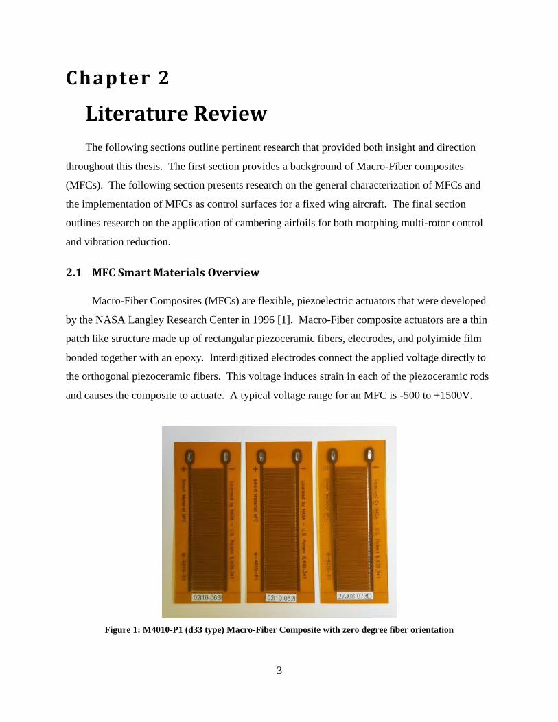
Macro-Fiber Composites (MFCs) are flexible, piezoelectric actuators that were developed

by the NASA Langley Research Center in 1996 [1]. Macro-Fiber composite actuators are a thin

patch like structure made up of rectangular piezoceramic fibers, electrodes, and polyimide film

bonded together with an epoxy. Interdigitized electrodes connect the applied voltage directly to

the orthogonal piezoceramic fibers. This voltage induces strain in each of the piezoceramic rods

and causes the composite to actuate. A typical voltage range for an MFC is -500 to +1500V.

Figure 1: M4010-P1 (d33 type) Macro-Fiber Composite with zero degree fiber orientation

4

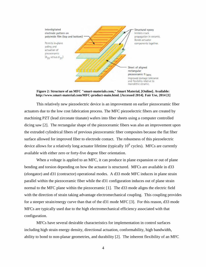
Figure 2: Structure of an MFC "smart-materials.com," Smart Material, [Online]. Available:

http://www.smart-material.com/MFC-product-main.html. [Accessed 2014]. Fair Use, 2014 [1]

This relatively new piezoelectric device is an improvement on earlier piezoceramic fiber

actuators due to the low cost fabrication process. The MFC piezoelectric fibers are created by

machining PZT (lead zirconate titanate) wafers into fiber sheets using a computer controlled

dicing saw [2]. The rectangular shape of the piezoceramic fibers was also an improvement upon

the extruded cylindrical fibers of previous piezoceramic fiber composites because the flat fiber

surface allowed for improved fiber to electrode contact. The robustness of this piezoelectric

device allows for a relatively long actuator lifetime (typically 108 cycles). MFCs are currently

available with either zero or forty-five degree fiber orientation.

When a voltage is applied to an MFC, it can produce in plane expansion or out of plane

bending and torsion depending on how the actuator is structured. MFCs are available in d33

(elongator) and d31 (contractor) operational modes. A d33 mode MFC induces in plane strain

parallel within the piezoceramic fiber while the d31 configuration induces out of plane strain

normal to the MFC plane within the piezoceramic [1]. The d33 mode aligns the electric field

with the direction of strain taking advantage electromechanical coupling. This coupling provides

for a steeper strain/energy curve than that of the d31 mode MFC [3]. For this reason, d33 mode

MFCs are typically used due to the high electromechanical efficiency associated with that

configuration.

MFCs have several desirable characteristics for implementation in control surfaces

including high strain energy density, directional actuation, conformability, high bandwidth,

ability to bond to non-planar geometries, and durability [2]. The inherent flexibility of an MFC

5

allows it to be bonded to curved surfaces unlike many monolithic piezoceramic materials. This

conforming property makes MFCs an excellent candidate as an actuator for a variety of

applications like vibration suppression, morphing surfaces, and flow control. In addition to

being extremely flexible, MFCs have a relatively high unloaded bandwidth in comparison to

conventional servos allowing for fast response time when used in control applications. MFCs

can also be used in converse for applications like an energy harvesting device, or an extremely

sensitive strain gauge due to their ability to produce higher voltages.

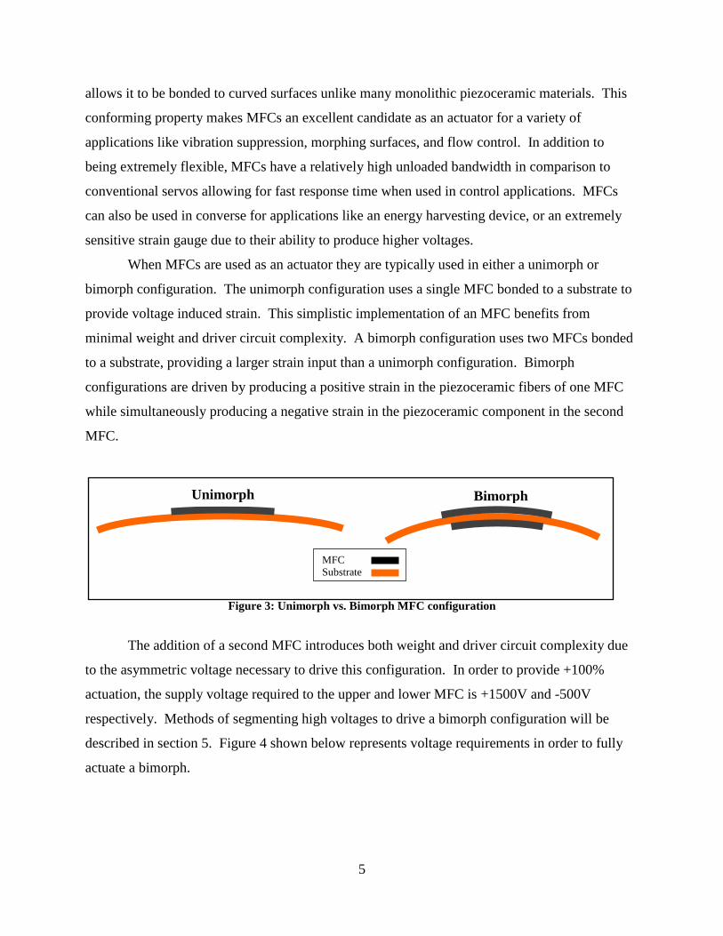
When MFCs are used as an actuator they are typically used in either a unimorph or

bimorph configuration. The unimorph configuration uses a single MFC bonded to a substrate to

provide voltage induced strain. This simplistic implementation of an MFC benefits from

minimal weight and driver circuit complexity. A bimorph configuration uses two MFCs bonded

to a substrate, providing a larger strain input than a unimorph configuration. Bimorph

configurations are driven by producing a positive strain in the piezoceramic fibers of one MFC

while simultaneously producing a negative strain in the piezoceramic component in the second

MFC.

Figure 3: Unimorph vs. Bimorph MFC configuration

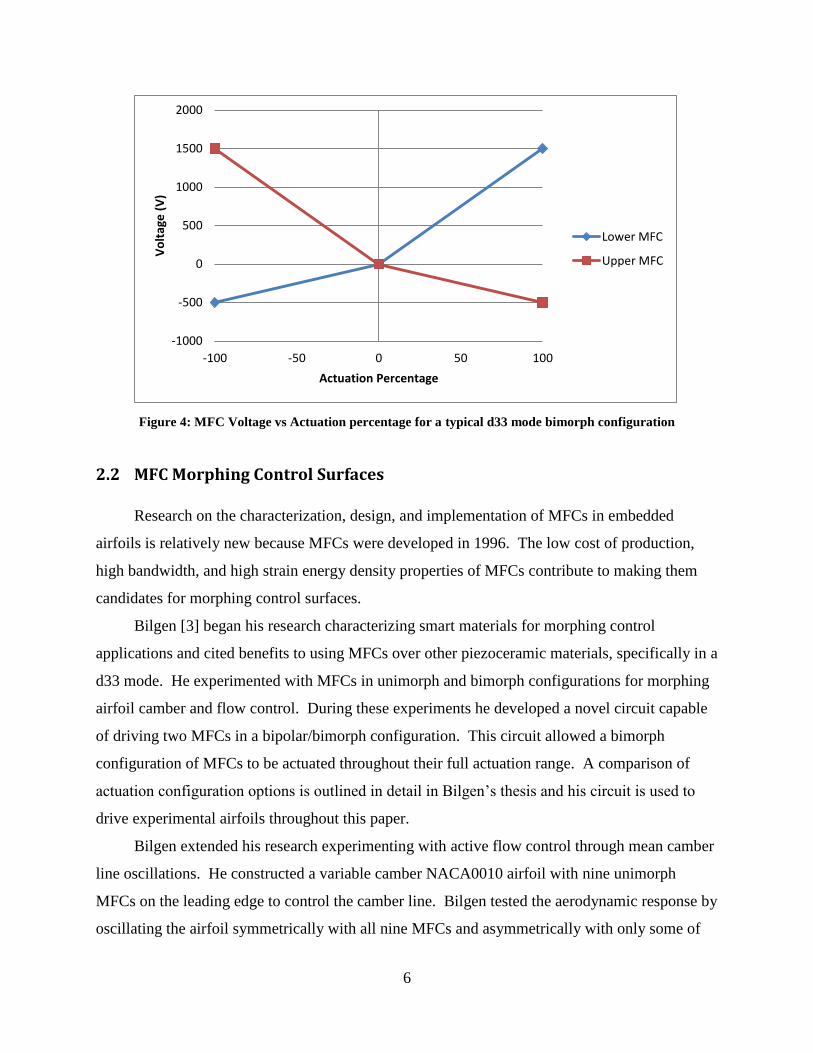
The addition of a second MFC introduces both weight and driver circuit complexity due

to the asymmetric voltage necessary to drive this configuration. In order to provide +100%

actuation, the supply voltage required to the upper and lower MFC is +1500V and -500V

respectively. Methods of segmenting high voltages to drive a bimorph configuration will be

described in section 5. Figure 4 shown below represents voltage requirements in order to fully

actuate a bimorph.

Bimorph Unimorph

MFC

Substrate

6

Figure 4: MFC Voltage vs Actuation percentage for a typical d33 mode bimorph configuration

2.2 MFC Morphing Control Surfaces

Research on the characterization, design, and implementation of MFCs in embedded

airfoils is relatively new because MFCs were developed in 1996. The low cost of production,

high bandwidth, and high strain energy density properties of MFCs contribute to making them

candidates for morphing control surfaces.

Bilgen [3] began his research characterizing smart materials for morphing control

applications and cited benefits to using MFCs over other piezoceramic materials, specifically in a

d33 mode. He experimented with MFCs in unimorph and bimorph configurations for morphing

airfoil camber and flow control. During these experiments he developed a novel circuit capable

of driving two MFCs in a bipolar/bimorph configuration. This circuit allowed a bimorph

configuration of MFCs to be actuated throughout their full actuation range. A comparison of

actuation configuration options is outlined in detail in Bilgen’s thesis and his circuit is used to

drive experimental airfoils throughout this paper.

Bilgen extended his research experimenting with active flow control through mean camber

line oscillations. He constructed a variable camber NACA0010 airfoil with nine unimorph

MFCs on the leading edge to control the camber line. Bilgen tested the aerodynamic response by

oscillating the airfoil symmetrically with all nine MFCs and asymmetrically with only some of

-1000

-500

0

500

1000

1500

2000

-100 -50 0 50 100

Vo

ltag

e (

V)

Actuation Percentage

Lower MFC

Upper MFC

7

the actuators. By oscillating the leading edge of this test airfoil, Bilgen was able to increase the

lift coefficient in the post stall region by 27.5% while actuating the leading edge at 125 Hz with a

flow rate of 5 m/s.

Gustafson [4] studied the structural properties of laminate composites for thin profile

MAV morphing wing design. He developed an FEA model of MFCs using a thermal analogy

for piezoelectric strain. Using this model he simulated the deformation, lift, and drag

characteristics of a novel thin GenMAV airfoil with MFC morphing camber. Gustafson later

constructed this airfoil for wind tunnel testing to compare with his model. Through 2D wind

tunnel testing, he measured aerodynamic loading under static deflections along with lift and

drag. As a further proof of concept that MFC bimorph implementation in a MAV was feasible,

Gustafson developed a flight weight circuit capable of driving MFC bimorphs that only weighed

23 grams.

Probst [5] expanded on Gustafson’s research and compared an airfoil with trailing edge

MFC camber control to conventional servomechanism ailerons used on UAVs. Theoretically,

the MFC camber controlled airfoil should have been more efficient than the servomechanism due

to the continuous surface contour. Probst’s experiments showed the servomechanism achieved a

higher L/D efficiency but noted that the MFC was not actuating at the same camber percentage

as the servomechanism. He noted that the aeroelastic deflection of the loaded MFC airfoil

changed the overall camber to be less than that of the servomechanism.

Probst rapid prototyped a continuously cambered airfoil (resembling the MFC airfoil) and

a conventional actuated aileron shape airfoil. The rapid prototyped airfoils were sufficiently stiff

enough that aerodynamic loading did not alter the contour of either airfoil. After rerunning his

experiment, Probst found that the continuous airfoil was more efficient. Probst mentioned a need

to take aeroelastic effects into account during the design of MFC control surfaces to correct for

changes in camber due to aerodynamic loading. After wind tunnel tests, Probst simulated a thin

wing with MFC’s in different configurations. He used a FEA to determine the optimal location

and configuration MFCs control surfaces for roll authority. Probst, along with researchers from

AVID LLC constructed and tested this thin winged design and compared it to the simulated

results.

Kim and Han [6] developed a flight mechanism with MFCs morphing control surfaces in

an ornithopter configuration to mimic the flight mechanisms of birds and insects. The MFCs

8

provide a camber control input into the flapping wing design while an electric motor creates the

flapping motion. Kim and Han experiment with various flapping frequencies and air speeds.

They show that the lift generated by the flapping wing can be increased by 20% when the MFCs

camber control is included in the flapping wing vehicle.

2.3 Alternative Oscillatory Camber Mechanisms

Research to use oscillatory surfaces on helicopter rotors for the purpose of harmonic

control is not new. Duffy, Nickerson, and Colasante [7] experimented with a 12 percent thick

modified VR-7 airfoil from a four foot section of the Boeing CH-47 Chinook helicopter blade to

evaluate the feasibility of a higher harmonic control surface embedded in a rotor. The snap

through airfoil design had a pneumatic actuator and two bar linkage on the interior that altered

the lower airfoil surface aft of the D box by snapping the lower surface in toward the centerline

of the airfoil. A preliminary second order vortex panel analysis of the airfoil showed the snap

through mechanism was capable of increasing the coefficient of pressure across the airfoil and

subsequently the lift and nose-down pitching moment.

After integrating the pressure coefficient over the airfoil surface at various angles of attack,

Duffy determined that direct cyclic pitch control via the snap through mechanism and a rigid

rotor blade was not possible because the coefficient of lift only increased by 0.06 when the

mechanism was fully actuated compared to the unactuated airfoil. After integrating the load

distributions along the rotor blade, Duffy found that the reduction in lift due to the twist induced

in the rotor blade from the nose down pitching moment dominated the slight increase in lift due

to the camber change in the snap through airfoil. Although the snap through panel mechanism

could not be used to control the rotor directly, it was found that the elastic twist induced in the

rotor from the nose-down pitching moment effectively reduced the overall blade lift, and this

reduction in overall blade lift could potentially be used for cyclic control.

Oscillatory morphing of the airfoil camber line has also been used for wake vortex

mitigation and active control of airfoil flow separation. Pern and Jacob [8] utilized a modified

NACA 4415 airfoil with a THUNDER piezo-ceramic actuator mounted beneath the surface of

the airfoil to modify the curvature of the upper surface ±0.2𝑚𝑚. Pern conducted preliminary

9

experiments on this airfoil, measuring the velocity deficit and vorticity fields in an initial study

of the airfoil’s potential for wake vortex mitigation.

Munday and Jacob [9] expanded on this work measuring force and particle image

velocimetry of the airfoil in static conditions with intermediate and maximum upper surface

displacements which resulted in a L/D decrease of 6% and increase in 2% respectively. After

preliminary testing, they oscillated the upper surface at frequencies between 0 and 11 Hz in low

Reynolds number conditions at various angles of attack. Through smoke wire flow visualization

they were able to show that oscillating the curvature of the upper surface effectively reduced

flow separation by as much as 30-60% at angles of attack up to 9 degrees. He notes that the

point of flow separation is comparatively the same between both the actuated and unactuated

cases and that since the region of camber oscillation is downstream of the separation point, the

actuation in not affecting the upstream flow directly. They theorized that the surface oscillations

are aiding the flow in navigating the adverse pressure gradient in the separation region by

energizing the boundary layer.

Clement [10] conducted a bench top and preliminary wind tunnel analysis of an active

rotor blade flap. He constructed a modified twelve inch NACA 0012 airfoil with a trailing edge

flap as the platform for his experiments. Actuation of the rotor flap was conducted using a novel

structure of C-Block piezoelectric actuators stacked horizontally within the rotor body. These

actuators provide deflection of the trailing edge flap that is 10% of the chord through a series of

brass shims. The C-Block actuators provided small trailing edge flap deflections with a

maximum deflection of approximately 100 µm recorded corresponding to 6 degrees of angular

deflection. Maximum blocking forces of approximately 10 N were recorded for the trailing edge

while actuating the trailing edge and simultaneously forcing the trailing edge to return to zero

deflection. Clement mentions the need for precise location of the center of pressure on the spar

axis to reduce an induced moment in the airfoil.

Garcia [11] created a state space model for a helicopter rotor with blade mounted actuators

and evaluated the use of servo flaps for higher harmonic control in helicopter blades. Garcia’s

state space model is based on the use of Multi-Blade Coordinates (MBCs) and a lumped

torsional approximation of each rotor blade. He validated this state space model using Boeing’s

C60 aeroelastic rotor analysis program. Garcia characterized requirements for a HHC system by

determining the servo-flap loading and deflection for 0.25g of HHC authority. He compares this

10

actuation scheme to the HHC loading and deflection of a conventional root pitch control

mechanism. Garcia goes on to explain the extreme benefit of using servo-flaps for HHC rather

than root pitch actuation is the reduction of control loads necessary for vibration suppression.

Finally, he presents a multivariable linear quadratic regulator in conjunction with his rotor model

that could be used for HHC.

Straub and Merkley [12] developed plans and actuator requirements for a servo flap

mechanism to camber rotor mounted servo flaps. Using typical flight conditions for an AH-64

helicopter, they developed a set of physical target requirements for linear and torsional loading

factors, cyclical actuation rate, thermal environmental conditions, ruggedness, power

requirements, weight, and size. In addition to creating a list of physical target specifications,

qualitative design constraints like ease of maintainability are considered. The proposed design

for the servo flap mechanism consists of a linear actuator mounted in the plane of the blade spar

combined with a hydraulic piston to actuate the blade mounted flap. Smart materials considered

for the linear actuator include piezoelectric stack actuators, magnetostrictive, and shape memory

alloys (SMAs).

11

Chapter 3

3 Wind Tunnel Facility

The following section describes the wind tunnel test facility used to collect data for all

aerodynamic experiments. A summary of test equipment, calibration methods, data acquisition,

and test procedure is provided. The test airfoil is described and a summary of the construction

process is provided. Correlation of the airfoil lift with the oscillatory input is presented and

discussed. The method of determining the lift component due to cambering is explained.

3.1 Wind Tunnel Overview

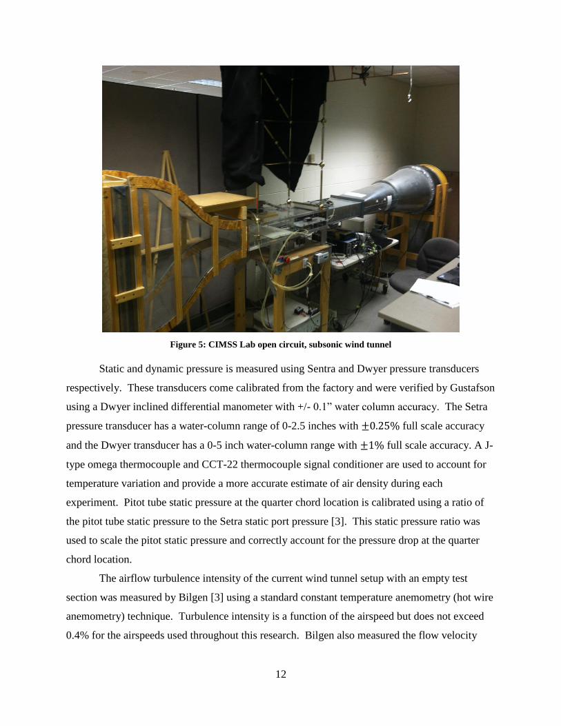
The wind tunnel used for all aerodynamic experiments presented in this research is an

open circuit, low air speed, apparatus tunnel built by Bilgen specifically for testing of

piezoelectric morphing airfoils and piezoelectric induced flow control as part of his PhD

dissertation. This apparatus is located in the CIMSS lab of Durham Hall at Virginia Polytechnic

Institute and State University and has also been used in experiments by both Gustafson and

Probst to collect experimental data for Macro-Fiber Composite embedded airfoils. The tunnel

body spans 4.1m in length and is constructed primarily of HVAC ducting and acrylic material.

Wind speeds from 2 m/s to 22 m/s are attainable with two cascaded AC fans that pull air

through a honeycomb flow straightener at the converging inlet of the wind tunnel. Air speed is

adjusted with a variable transformer to the desired speed at the beginning of each experiment.

Stability of the flow speed is dependent on the magnitude of the flow speed. This is described in

more detail in section A3 of the appendix. An acrylic test section that measures 136 mm tall by

365 mm wide allows for laser displacement measurements of the airfoil at multiple points on the

chord span and photography during MFC actuation. The acrylic also provides a smooth inner

surface to further mitigate undesirable turbulence at this critical section of the wind tunnel. A

seven inch diameter portal on both the ceiling and floor of the test section allow access into the

test section to install test samples.

12

Figure 5: CIMSS Lab open circuit, subsonic wind tunnel

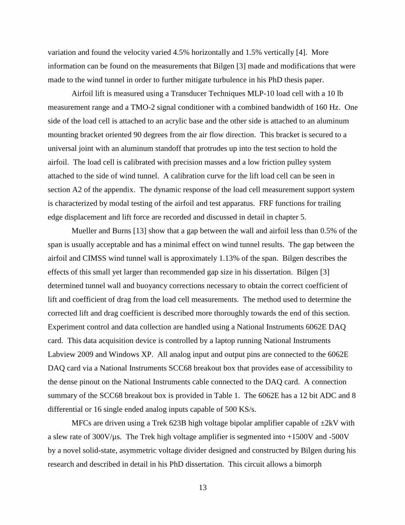
Static and dynamic pressure is measured using Sentra and Dwyer pressure transducers

respectively. These transducers come calibrated from the factory and were verified by Gustafson

using a Dwyer inclined differential manometer with +/- 0.1” water column accuracy. The Setra

pressure transducer has a water-column range of 0-2.5 inches with ±0.25% full scale accuracy

and the Dwyer transducer has a 0-5 inch water-column range with ±1% full scale accuracy. A J-

type omega thermocouple and CCT-22 thermocouple signal conditioner are used to account for

temperature variation and provide a more accurate estimate of air density during each

experiment. Pitot tube static pressure at the quarter chord location is calibrated using a ratio of

the pitot tube static pressure to the Setra static port pressure [3]. This static pressure ratio was

used to scale the pitot static pressure and correctly account for the pressure drop at the quarter

chord location.

The airflow turbulence intensity of the current wind tunnel setup with an empty test

section was measured by Bilgen [3] using a standard constant temperature anemometry (hot wire

anemometry) technique. Turbulence intensity is a function of the airspeed but does not exceed

0.4% for the airspeeds used throughout this research. Bilgen also measured the flow velocity

13

variation and found the velocity varied 4.5% horizontally and 1.5% vertically [4]. More

information can be found on the measurements that Bilgen [3] made and modifications that were

made to the wind tunnel in order to further mitigate turbulence in his PhD thesis paper.

Airfoil lift is measured using a Transducer Techniques MLP-10 load cell with a 10 lb

measurement range and a TMO-2 signal conditioner with a combined bandwidth of 160 Hz. One

side of the load cell is attached to an acrylic base and the other side is attached to an aluminum

mounting bracket oriented 90 degrees from the air flow direction. This bracket is secured to a

universal joint with an aluminum standoff that protrudes up into the test section to hold the

airfoil. The load cell is calibrated with precision masses and a low friction pulley system

attached to the side of wind tunnel. A calibration curve for the lift load cell can be seen in

section A2 of the appendix. The dynamic response of the load cell measurement support system

is characterized by modal testing of the airfoil and test apparatus. FRF functions for trailing

edge displacement and lift force are recorded and discussed in detail in chapter 5.

Mueller and Burns [13] show that a gap between the wall and airfoil less than 0.5% of the

span is usually acceptable and has a minimal effect on wind tunnel results. The gap between the

airfoil and CIMSS wind tunnel wall is approximately 1.13% of the span. Bilgen describes the

effects of this small yet larger than recommended gap size in his dissertation. Bilgen [3]

determined tunnel wall and buoyancy corrections necessary to obtain the correct coefficient of

lift and coefficient of drag from the load cell measurements. The method used to determine the

corrected lift and drag coefficient is described more thoroughly towards the end of this section.

Experiment control and data collection are handled using a National Instruments 6062E DAQ

card. This data acquisition device is controlled by a laptop running National Instruments

Labview 2009 and Windows XP. All analog input and output pins are connected to the 6062E

DAQ card via a National Instruments SCC68 breakout box that provides ease of accessibility to

the dense pinout on the National Instruments cable connected to the DAQ card. A connection

summary of the SCC68 breakout box is provided in Table 1. The 6062E has a 12 bit ADC and 8

differential or 16 single ended analog inputs capable of 500 KS/s.

MFCs are driven using a Trek 623B high voltage bipolar amplifier capable of ±2kV with

a slew rate of 300V/µs. The Trek high voltage amplifier is segmented into +1500V and -500V

by a novel solid-state, asymmetric voltage divider designed and constructed by Bilgen during his

research and described in detail in his PhD dissertation. This circuit allows a bimorph

14

configuration of MFCs to be driven from a single amplifier. A signal voltage from Labview is

used to scale the amplifier output voltage to provide variations in output amplitude.

In order to collect wind tunnel data while also actuating the airfoil MFCs, the Labview VI

architecture necessary to run the wind tunnel was reconfigured on a new laptop and modified to

send an actuation signal while simultaneously collecting data from all of the sensors used in the

experiment. Camber oscillations are produced by implementing the amplifier control signal as a

sine wave with a user specified amplitude and frequency.

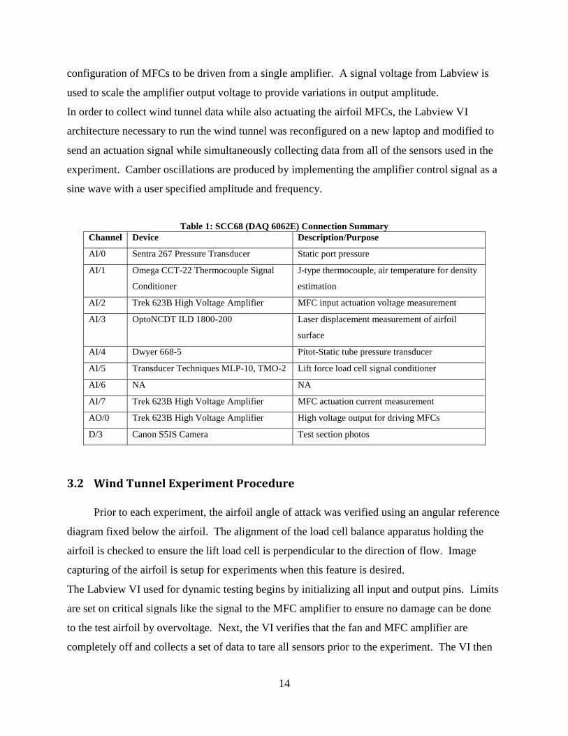
Table 1: SCC68 (DAQ 6062E) Connection Summary

Channel Device Description/Purpose

AI/0 Sentra 267 Pressure Transducer Static port pressure

AI/1 Omega CCT-22 Thermocouple Signal

Conditioner

J-type thermocouple, air temperature for density

estimation

AI/2 Trek 623B High Voltage Amplifier MFC input actuation voltage measurement

AI/3 OptoNCDT ILD 1800-200 Laser displacement measurement of airfoil

surface

AI/4 Dwyer 668-5 Pitot-Static tube pressure transducer

AI/5 Transducer Techniques MLP-10, TMO-2 Lift force load cell signal conditioner

AI/6 NA NA

AI/7 Trek 623B High Voltage Amplifier MFC actuation current measurement

AO/0 Trek 623B High Voltage Amplifier High voltage output for driving MFCs

D/3 Canon S5IS Camera Test section photos

3.2 Wind Tunnel Experiment Procedure

Prior to each experiment, the airfoil angle of attack was verified using an angular reference

diagram fixed below the airfoil. The alignment of the load cell balance apparatus holding the

airfoil is checked to ensure the lift load cell is perpendicular to the direction of flow. Image

capturing of the airfoil is setup for experiments when this feature is desired.

The Labview VI used for dynamic testing begins by initializing all input and output pins. Limits

are set on critical signals like the signal to the MFC amplifier to ensure no damage can be done

to the test airfoil by overvoltage. Next, the VI verifies that the fan and MFC amplifier are

completely off and collects a set of data to tare all sensors prior to the experiment. The VI then

15

asks for the user to input a voltage amplitude and actuation frequency for the MFCs as well as

the desired airspeed.

After setting up the experiment conditions the user manually sets the airspeed to the

desired value using a variable transformer and starts the experiment. Data is collected and saved

to a folder based on the time and date of the experiment and then subdivided into folders based

on air speed, MFC actuation frequency, and amplitude. Finally, a post experiment set of data is

collected to verification all sensors did not deviate significantly from the initial tare. Additional

settings to automatically take photographs at various points during the experiment and to collect

hysteresis data after the experiment is complete are also included for convenience.

Limitations on the test section dimensions create boundary conditions that do not

accurately represent free stream conditions. Since airflow around the airfoil does not perfectly

represent free stream conditions, a correction factor (kCL) is included when calculating the

coefficient of lift. The corrected lift coefficient when this factor is included is defined as

follows:

𝐶𝑙 = 𝑘𝐶𝑙𝐶𝑙𝑢

(E3.1)

Where: 𝐶𝑙: Coefficient of Lift

𝐶𝑙𝑢: Uncorrected Coefficient of Lift

𝑘𝐶𝑙: Correction factor

The lift coefficient correction factor described by Barlow [14] is similar to the method of

images, where singularities are arranged to simulate real wall boundaries in a flow field. The

described correction method is documented and has been used by both Bilgen [3] and Gustafson

[4] in their research. The uncorrected lift coefficient is calculated using the standard lift equation

shown below.

16

𝐶𝑙𝑢 =2𝐿

𝜌𝑣2𝑆 (E3.2)

Where: 𝐶𝑙𝑢: Uncorrected Coefficient of Lift

L: Lift Force

𝜌: Air Density

S: Airfoil Planform Area

𝑣: Airspeed

The correction factor is calculated via solid ϵ𝑠𝑏 and wake blockage 𝜖𝜔𝑏 terms that account for a

variation in free stream airspeed due to the volume of the airfoil and the downstream wake

respectively [15]. The solid and wake blockage terms were measured by Probst [5] using the

same wind tunnel and airfoil.

𝑘𝐶𝑙 = 1 − 𝜎 − 2ϵ𝑠𝑏 − 2𝜖𝜔𝑏 (E3.3)

Where:

𝑘𝐶𝑙: Coefficient of lift correction factor

𝜎: Wind tunnel correction parameter

ϵ𝑠𝑏: Solid Blockage term

𝜖𝜔𝑏: Wake blockage term

A streamline curvature correction for the angle of attack is included to account for

variation in the incidence angle of freestream flow do to the presence of the airfoil within the

wind tunnel [15]. This correction is implemented using XFOIL data obtained for the moment

coefficient. The following equation outlines the streamline curvature correction where αsc is the

streamline curvature correction and Cm is the moment coefficient at the quarter chord for each

static actuation test of the airfoil. This correction factor is added to the angle of attack in the

results found in section 6 to better represent wind tunnel test conditions.

17

𝛼𝑠𝑐 =𝜎

2𝜋(𝐶𝑙𝑢 − 4𝐶𝑚)

(E3.4)

Where: 𝐶𝑙𝑢: Uncorrected Coefficient of Lift

𝐶𝑚: Moment coefficient at quarter chord

𝜎: Wind tunnel correction parameter

𝛼𝑠𝑐: Streamline Curvature Correction

The streamline curvature correction and the corrected coefficient of lift are both partially

made up of a wind tunnel correction parameter that relates the ratio of the chord to the wind

tunnel height. This correction parameter is listed in the equation below.

𝜎 =

𝜋2𝑐2

48ℎ2

(E3.5)

Where: 𝜎: Wind tunnel correction parameter

ℎ: Test section height

𝑐: Chord length

Three dimensional flow corrections for the finite width of the airfoil’s vertical span were

not incorporated in the following analysis. As a result, at higher coefficient of lift configurations

there is more error associated with the measured coefficient of lift. This is due to a steeper

gradient in the elliptical lift distribution of a finite airfoil that results from a high coefficient of

lift configuration [16].

18

Chapter 4

4 Test Airfoil

4.1 Test Airfoil Description

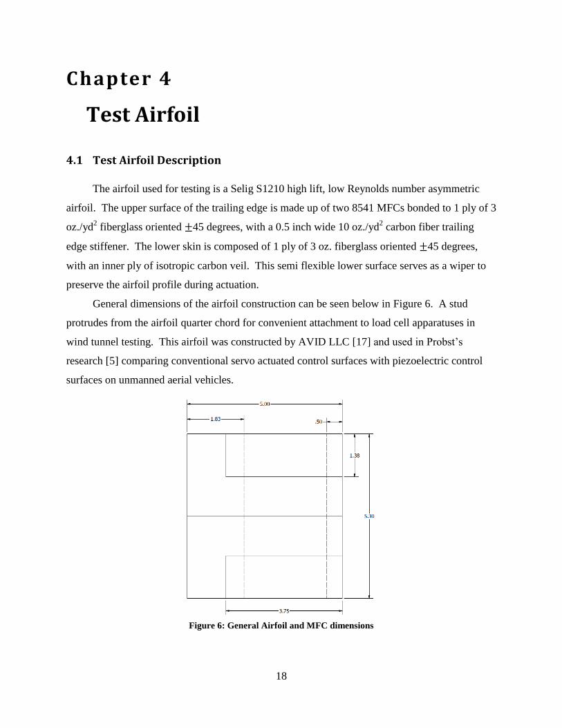
The airfoil used for testing is a Selig S1210 high lift, low Reynolds number asymmetric

airfoil. The upper surface of the trailing edge is made up of two 8541 MFCs bonded to 1 ply of 3

oz./yd2 fiberglass oriented ±45 degrees, with a 0.5 inch wide 10 oz./yd

2 carbon fiber trailing

edge stiffener. The lower skin is composed of 1 ply of 3 oz. fiberglass oriented ±45 degrees,

with an inner ply of isotropic carbon veil. This semi flexible lower surface serves as a wiper to

preserve the airfoil profile during actuation.

General dimensions of the airfoil construction can be seen below in Figure 6. A stud

protrudes from the airfoil quarter chord for convenient attachment to load cell apparatuses in

wind tunnel testing. This airfoil was constructed by AVID LLC [17] and used in Probst’s

research [5] comparing conventional servo actuated control surfaces with piezoelectric control

surfaces on unmanned aerial vehicles.

Figure 6: General Airfoil and MFC dimensions

19

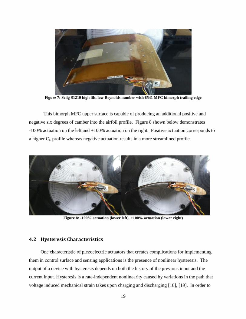
Figure 7: Selig S1210 high lift, low Reynolds number with 8541 MFC bimorph trailing edge

This bimorph MFC upper surface is capable of producing an additional positive and

negative six degrees of camber into the airfoil profile. Figure 8 shown below demonstrates

-100% actuation on the left and +100% actuation on the right. Positive actuation corresponds to

a higher CL profile whereas negative actuation results in a more streamlined profile.

Figure 8: -100% actuation (lower left), +100% actuation (lower right)

4.2 Hysteresis Characteristics

One characteristic of piezoelectric actuators that creates complications for implementing

them in control surface and sensing applications is the presence of nonlinear hysteresis. The

output of a device with hysteresis depends on both the history of the previous input and the

current input. Hysteresis is a rate-independent nonlinearity caused by variations in the path that

voltage induced mechanical strain takes upon charging and discharging [18], [19]. In order to

20

prevent actuation errors, control systems must include a compensator to account for hysteresis in

the control systems architecture. The use of hysteresis operators like Preisach and

Prandtl-Ishilinskii for real time hysteresis compensation in control systems is a prevalent

research topic [20], [21]. Compensation algorithms implemented in series with piezoelectric

actuator models can produce relatively accurate linear models that are sufficient for many

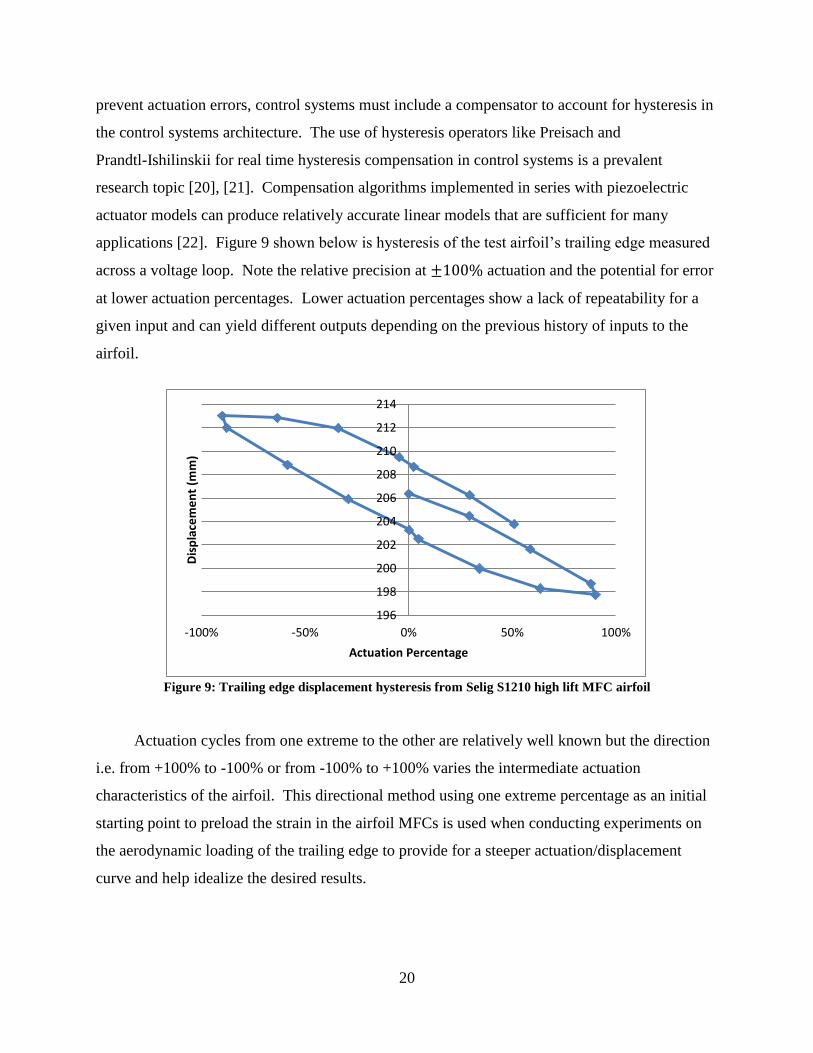
applications [22]. Figure 9 shown below is hysteresis of the test airfoil’s trailing edge measured

across a voltage loop. Note the relative precision at ±100% actuation and the potential for error

at lower actuation percentages. Lower actuation percentages show a lack of repeatability for a

given input and can yield different outputs depending on the previous history of inputs to the

airfoil.

Figure 9: Trailing edge displacement hysteresis from Selig S1210 high lift MFC airfoil

Actuation cycles from one extreme to the other are relatively well known but the direction

i.e. from +100% to -100% or from -100% to +100% varies the intermediate actuation

characteristics of the airfoil. This directional method using one extreme percentage as an initial

starting point to preload the strain in the airfoil MFCs is used when conducting experiments on

the aerodynamic loading of the trailing edge to provide for a steeper actuation/displacement

curve and help idealize the desired results.

196

198

200

202

204

206

208

210

212

214

-100% -50% 0% 50% 100%

Dis

pla

cem

en

t (m

m)

Actuation Percentage

21

4.3 Definition of Support Angle

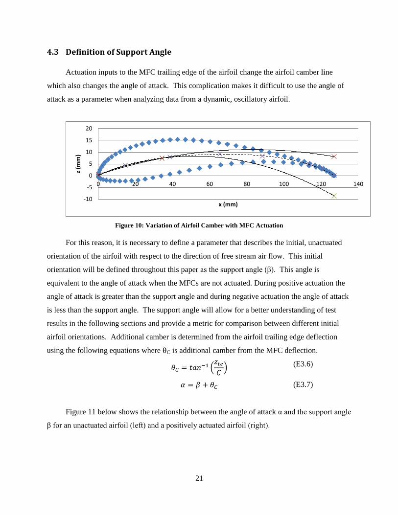
Actuation inputs to the MFC trailing edge of the airfoil change the airfoil camber line

which also changes the angle of attack. This complication makes it difficult to use the angle of

attack as a parameter when analyzing data from a dynamic, oscillatory airfoil.

Figure 10: Variation of Airfoil Camber with MFC Actuation

For this reason, it is necessary to define a parameter that describes the initial, unactuated

orientation of the airfoil with respect to the direction of free stream air flow. This initial

orientation will be defined throughout this paper as the support angle (β). This angle is

equivalent to the angle of attack when the MFCs are not actuated. During positive actuation the

angle of attack is greater than the support angle and during negative actuation the angle of attack

is less than the support angle. The support angle will allow for a better understanding of test

results in the following sections and provide a metric for comparison between different initial

airfoil orientations. Additional camber is determined from the airfoil trailing edge deflection

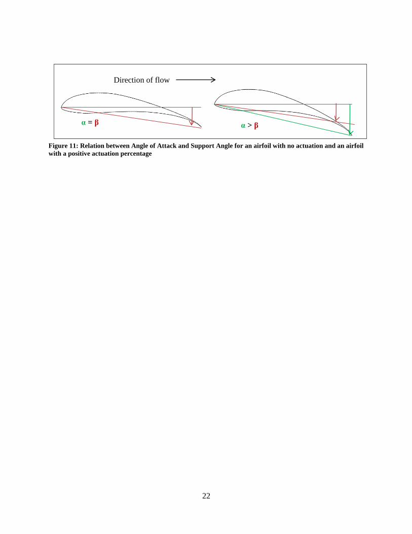
using the following equations where θC is additional camber from the MFC deflection.

𝜃𝐶 = 𝑡𝑎𝑛−1 (𝑧𝑡𝑒𝐶)

(E3.6)

𝛼 = 𝛽 + 𝜃𝐶 (E3.7)

Figure 11 below shows the relationship between the angle of attack α and the support angle

β for an unactuated airfoil (left) and a positively actuated airfoil (right).

-10

-5

0

5

10

15

20

0 20 40 60 80 100 120 140

z (m

m)

x (mm)

22

Figure 11: Relation between Angle of Attack and Support Angle for an airfoil with no actuation and an airfoil

with a positive actuation percentage

α = β α > β

Direction of flow

23

Chapter 5

5 Modal Testing

This section describes the experimental procedure for modal testing of the airfoil and the

wind tunnel measurement apparatus used to collect lift data. Modal testing of the airfoil was

conducted prior to testing the airfoil in the wind tunnel. The goals of modal testing were both

preventative and exploratory. One objective of the modal analysis was to highlight resonant

frequencies to prevent coupling of the MFC actuators with the airfoil dynamics which could lead

to destructive behavior of the test airfoil. Another goal was to explore mode shapes of the test

airfoil and load cell apparatus to better understand the frequency response results from wind

tunnel testing. Finally, the effect of static MFC actuation on the shape of the frequency response

function is presented.

5.1 Modal Testing Description

The frequency response function of the combined airfoil and test apparatus was measured

by applying an impulse to the airfoil with a modal hammer and measuring the velocity of the

airfoil with a laser doppler vibrometer. Impulses were provided by a Dytran model 5800SL,

Ultra Miniature Impulse Hammer at the quarter chord and 50% vertical intersection. This

location is on the basswood of the airfoil and provides a better surface to excite modes of the

airfoil than the composite trailing edge. Velocity was captured using a Polytech PDV 100 set at

500 mm/s/V and recorded using SigLab, a data acquisition unit designed to interface seamlessly

with Matlab.

24

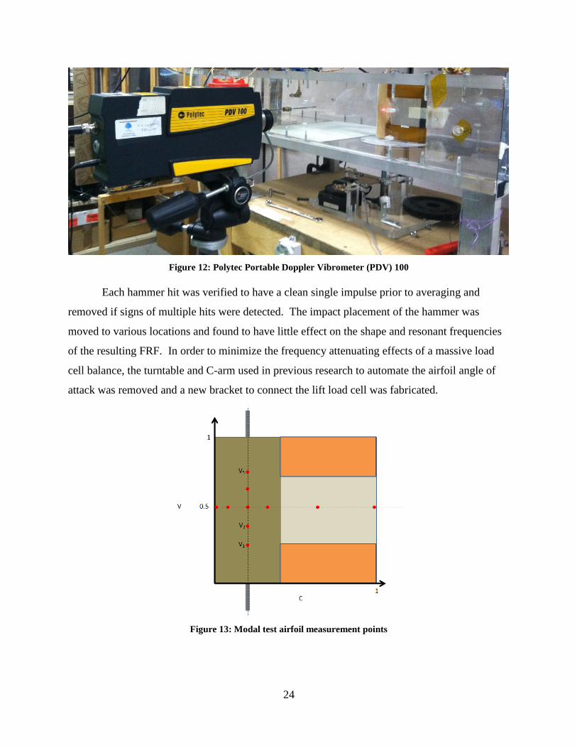
Figure 12: Polytec Portable Doppler Vibrometer (PDV) 100

Each hammer hit was verified to have a clean single impulse prior to averaging and

removed if signs of multiple hits were detected. The impact placement of the hammer was

moved to various locations and found to have little effect on the shape and resonant frequencies

of the resulting FRF. In order to minimize the frequency attenuating effects of a massive load

cell balance, the turntable and C-arm used in previous research to automate the airfoil angle of

attack was removed and a new bracket to connect the lift load cell was fabricated.

Figure 13: Modal test airfoil measurement points

25

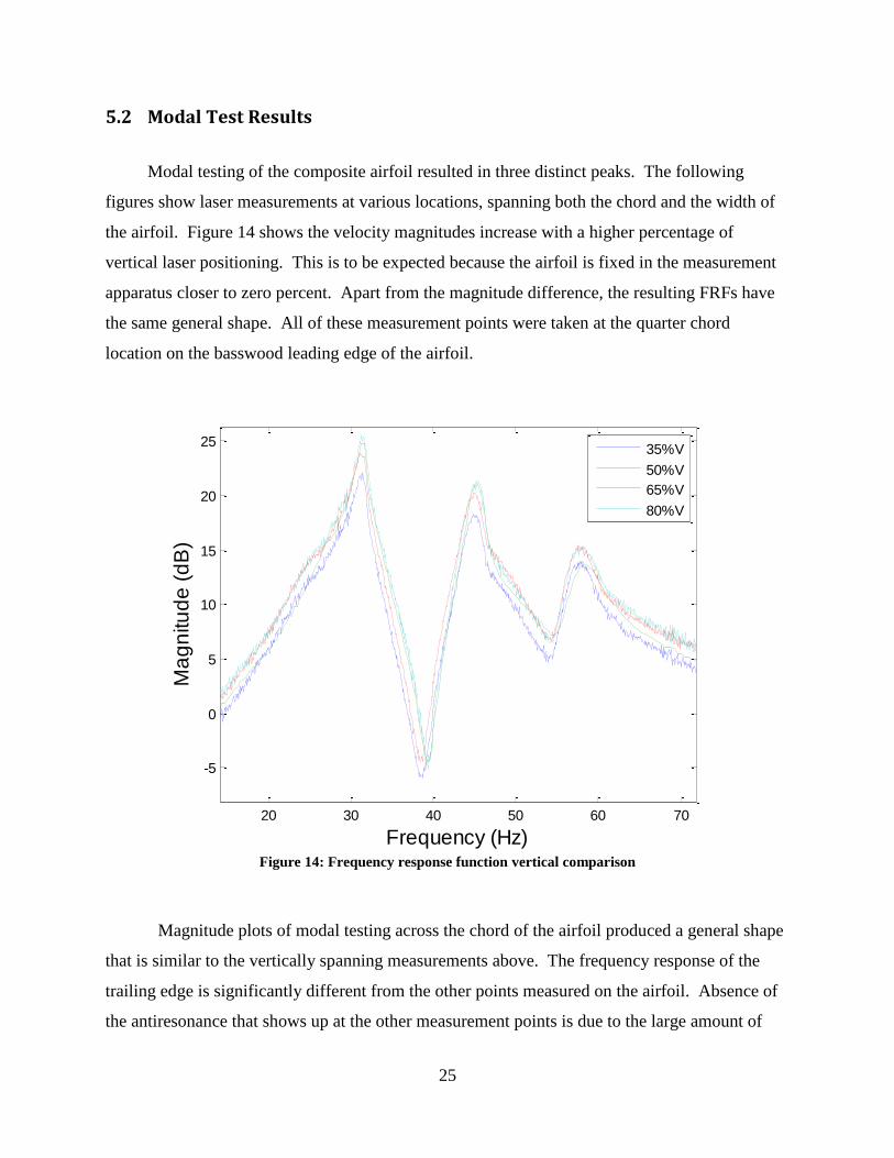
5.2 Modal Test Results

Modal testing of the composite airfoil resulted in three distinct peaks. The following

figures show laser measurements at various locations, spanning both the chord and the width of

the airfoil. Figure 14 shows the velocity magnitudes increase with a higher percentage of

vertical laser positioning. This is to be expected because the airfoil is fixed in the measurement

apparatus closer to zero percent. Apart from the magnitude difference, the resulting FRFs have

the same general shape. All of these measurement points were taken at the quarter chord

location on the basswood leading edge of the airfoil.

Figure 14: Frequency response function vertical comparison

Magnitude plots of modal testing across the chord of the airfoil produced a general shape

that is similar to the vertically spanning measurements above. The frequency response of the

trailing edge is significantly different from the other points measured on the airfoil. Absence of

the antiresonance that shows up at the other measurement points is due to the large amount of

20 30 40 50 60 70

-5

0

5

10

15

20

25

Frequency (Hz)

Ma

gn

itu

de

(d

B)

35%V

50%V

65%V

80%V

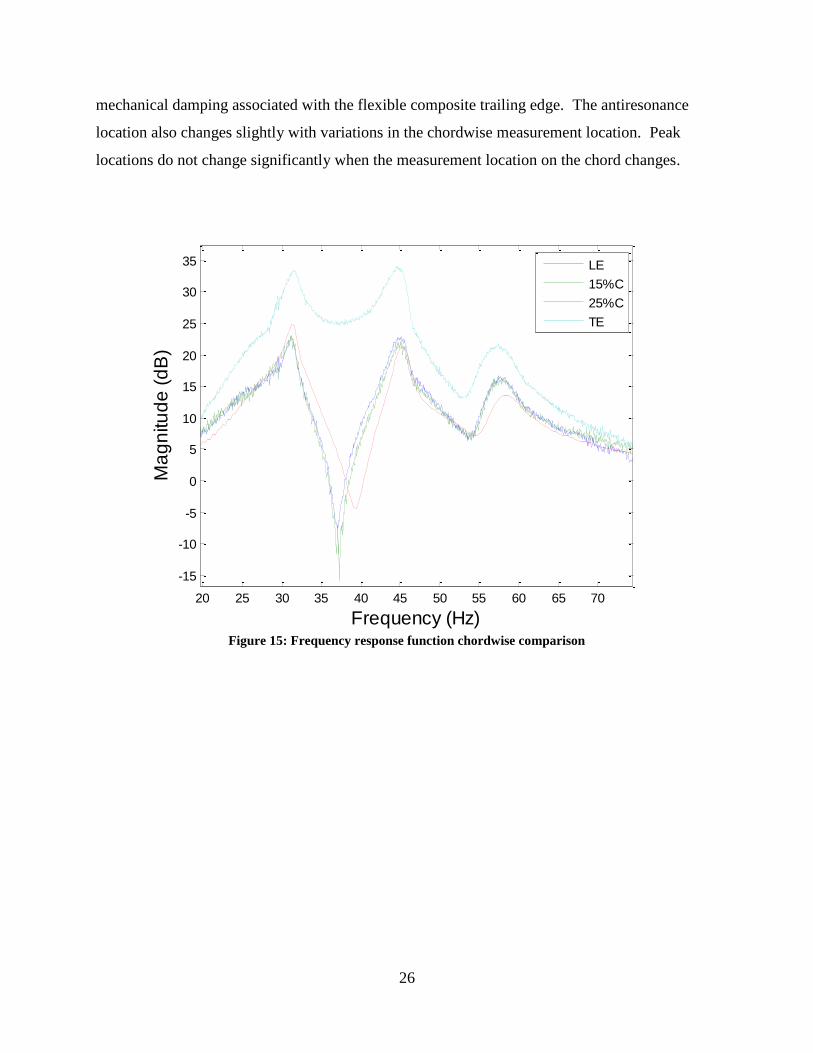
26

mechanical damping associated with the flexible composite trailing edge. The antiresonance

location also changes slightly with variations in the chordwise measurement location. Peak

locations do not change significantly when the measurement location on the chord changes.

Figure 15: Frequency response function chordwise comparison

20 25 30 35 40 45 50 55 60 65 70

-15

-10

-5

0

5

10

15

20

25

30

35

Frequency (Hz)

Ma

gn

itu

de

(d

B)

LE

15%C

25%C

TE

27

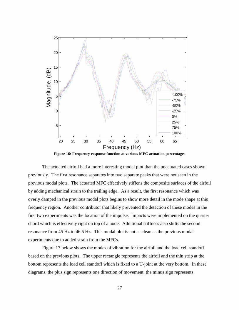
Figure 16: Frequency response function at various MFC actuation percentages

The actuated airfoil had a more interesting modal plot than the unactuated cases shown

previously. The first resonance separates into two separate peaks that were not seen in the

previous modal plots. The actuated MFC effectively stiffens the composite surfaces of the airfoil

by adding mechanical strain to the trailing edge. As a result, the first resonance which was

overly damped in the previous modal plots begins to show more detail in the mode shape at this

frequency region. Another contributor that likely prevented the detection of these modes in the

first two experiments was the location of the impulse. Impacts were implemented on the quarter

chord which is effectively right on top of a node. Additional stiffness also shifts the second

resonance from 45 Hz to 46.5 Hz. This modal plot is not as clean as the previous modal

experiments due to added strain from the MFCs.

Figure 17 below shows the modes of vibration for the airfoil and the load cell standoff

based on the previous plots. The upper rectangle represents the airfoil and the thin strip at the

bottom represents the load cell standoff which is fixed to a U-joint at the very bottom. In these

diagrams, the plus sign represents one direction of movement, the minus sign represents

20 25 30 35 40 45 50 55 60 65

-5

0

5

10

15

20

25

Frequency (Hz)

Ma

gn

itu

de

, (d

B)

-100%

-75%

-50%

-25%

0%

25%

75%

100%

28

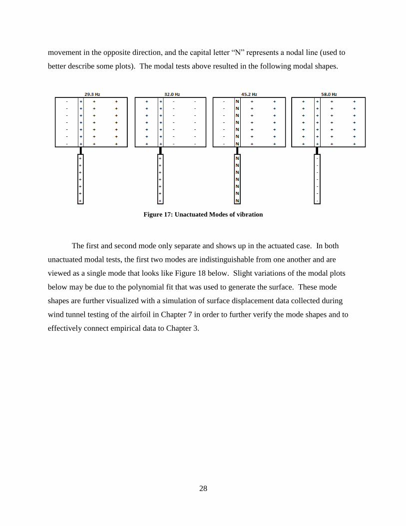
movement in the opposite direction, and the capital letter “N” represents a nodal line (used to

better describe some plots). The modal tests above resulted in the following modal shapes.

Figure 17: Unactuated Modes of vibration

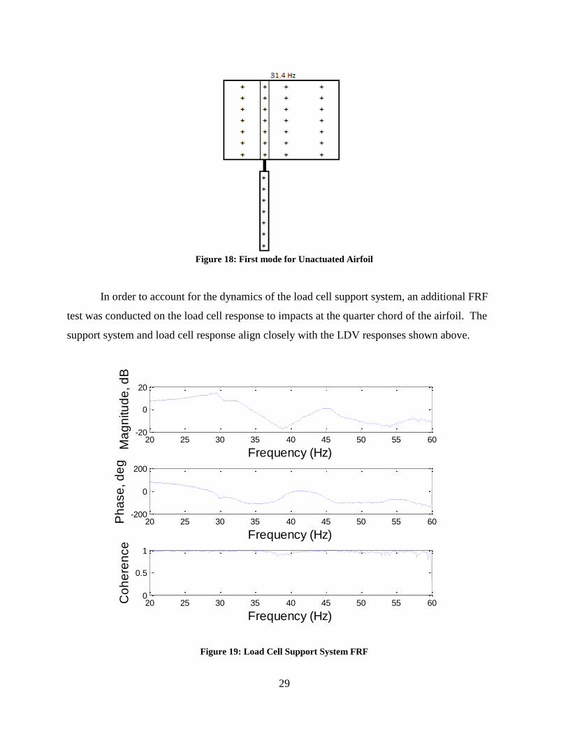
The first and second mode only separate and shows up in the actuated case. In both

unactuated modal tests, the first two modes are indistinguishable from one another and are

viewed as a single mode that looks like Figure 18 below. Slight variations of the modal plots

below may be due to the polynomial fit that was used to generate the surface. These mode

shapes are further visualized with a simulation of surface displacement data collected during

wind tunnel testing of the airfoil in Chapter 7 in order to further verify the mode shapes and to

effectively connect empirical data to Chapter 3.

29

Figure 18: First mode for Unactuated Airfoil

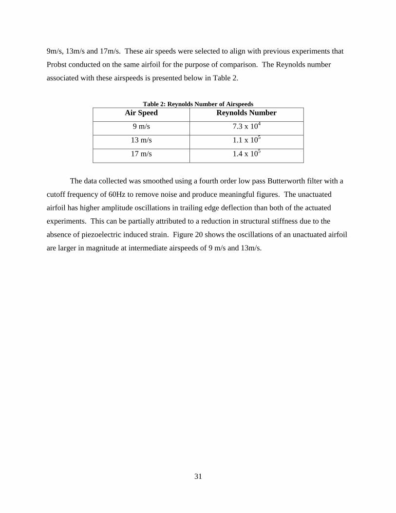
In order to account for the dynamics of the load cell support system, an additional FRF

test was conducted on the load cell response to impacts at the quarter chord of the airfoil. The

support system and load cell response align closely with the LDV responses shown above.

Figure 19: Load Cell Support System FRF

20 25 30 35 40 45 50 55 60-20

0

20

Frequency (Hz)

Ma

gn

itu

de

, d

B

20 25 30 35 40 45 50 55 60-200

0

200

Frequency (Hz)

Ph

ase

, d

eg

20 25 30 35 40 45 50 55 600

0.5

1

Frequency (Hz)

Co

he

ren

ce

30

Chapter 6

6 Wind Tunnel Results

Modal testing of the airfoil and load cell apparatus provided insight into some of the

occurrences that are recorded during wind tunnel testing. This chapter includes wind tunnel data

and post processing used to produce meaningful results from that data. Wind tunnel lift data

with both static and oscillatory MFC inputs was used to characterize aerodynamic loading and

frequency response information for various airspeeds and actuation frequencies. Coefficients of

lift plots are validated using a viscous XFOIL analysis of the airfoil at varying Reynolds

numbers and angles of attack.

6.1 Static Test Results

This section presents wind tunnel test results from static actuation inputs. The primary

motivation behind this section is to measure the effects of aerodynamic loading on the airfoil to

gain a better expectation of performance out of MFC morphing airfoils.

Aerodynamic loading on an MFC airfoil can have a prominent effect on the airfoil trailing edge

deflection and subsequently the lift that the airfoil can generate. Probst [5] mentioned these

effects while comparing MFC airfoils to conventional servomechanisms for the purpose of UAV

roll authority in fixed wing aircraft.

In order to measure the effect of aerodynamic loading on airfoil trailing edge deflection,

the displacement of the airfoil trailing edge was measured at various airspeeds while the MFCs

were actuated at a static 0%, +90% and -90% of their full actuation range. An initial support

angle of 0 degrees was selected to keep far below the airfoil stall region when the airfoil

actuated.

Prior to each experiment, the MFC’s hysteresis was accounted for by actuating the airfoil

fully +100% for the +90% trials and -100% for the -90% trials. It is important to note that the

0% actuation trials were conducted after the MFCs had been actuated to +100% so there may be

some positive actuation bias in these results. Each of the actuation amplitude was tested at 0m/s,

31

9m/s, 13m/s and 17m/s. These air speeds were selected to align with previous experiments that

Probst conducted on the same airfoil for the purpose of comparison. The Reynolds number

associated with these airspeeds is presented below in Table 2.

Table 2: Reynolds Number of Airspeeds

Air Speed Reynolds Number

9 m/s 7.3 x 104

13 m/s 1.1 x 105

17 m/s 1.4 x 105

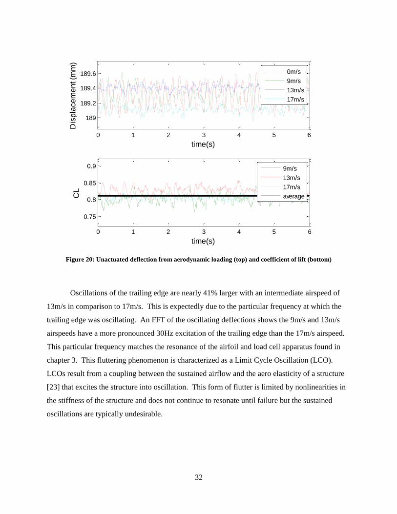
The data collected was smoothed using a fourth order low pass Butterworth filter with a

cutoff frequency of 60Hz to remove noise and produce meaningful figures. The unactuated

airfoil has higher amplitude oscillations in trailing edge deflection than both of the actuated

experiments. This can be partially attributed to a reduction in structural stiffness due to the

absence of piezoelectric induced strain. Figure 20 shows the oscillations of an unactuated airfoil

are larger in magnitude at intermediate airspeeds of 9 m/s and 13m/s.

32

Figure 20: Unactuated deflection from aerodynamic loading (top) and coefficient of lift (bottom)

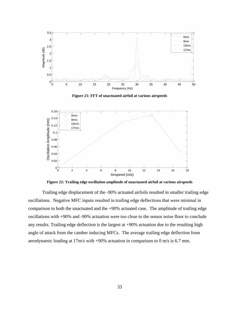
Oscillations of the trailing edge are nearly 41% larger with an intermediate airspeed of

13m/s in comparison to 17m/s. This is expectedly due to the particular frequency at which the

trailing edge was oscillating. An FFT of the oscillating deflections shows the 9m/s and 13m/s

airspeeds have a more pronounced 30Hz excitation of the trailing edge than the 17m/s airspeed.

This particular frequency matches the resonance of the airfoil and load cell apparatus found in

chapter 3. This fluttering phenomenon is characterized as a Limit Cycle Oscillation (LCO).

LCOs result from a coupling between the sustained airflow and the aero elasticity of a structure

[23] that excites the structure into oscillation. This form of flutter is limited by nonlinearities in

the stiffness of the structure and does not continue to resonate until failure but the sustained

oscillations are typically undesirable.

0 1 2 3 4 5 6

189

189.2

189.4

189.6

time(s)

Dis

pla

ce

me

nt (m

m)

0m/s

9m/s

13m/s

17m/s

0 1 2 3 4 5 6

0.75

0.8

0.85

0.9

time(s)

CL

9m/s

13m/s

17m/s

average

33

Figure 21: FFT of unactuated airfoil at various airspeeds

Figure 22: Trailing edge oscillation amplitude of unactuated airfoil at various airspeeds

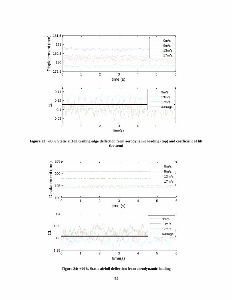
Trailing edge displacement of the -90% actuated airfoils resulted in smaller trailing edge

oscillations. Negative MFC inputs resulted in trailing edge deflections that were minimal in

comparison to both the unactuated and the +90% actuated case. The amplitude of trailing edge

oscillations with +90% and -90% actuation were too close to the sensor noise floor to conclude

any results. Trailing edge deflection is the largest at +90% actuation due to the resulting high

angle of attack from the camber inducing MFCs. The average trailing edge deflection from

aerodynamic loading at 17m/s with +90% actuation in comparison to 0 m/s is 6.7 mm.

0 5 10 15 20 25 30 35 40 45 500

0.5

1

1.5

2

2.5

3

3.5

Frequency (Hz)

Magnitude (

dB

)

0ms

9ms

13ms

17ms

0 2 4 6 8 10 12 14 16 180

0.02

0.04

0.06

0.08

0.1

0.12

0.14

0.16

Airspeed (m/s)

Oscilla

tio

n A

mp

litu

de

(m

m)

0m/s

9m/s

13m/s

17m/s

34

Figure 23: -90% Static airfoil trailing edge deflection from aerodynamic loading (top) and coefficient of lift

(bottom)

Figure 24: +90% Static airfoil deflection from aerodynamic loading

0 1 2 3 4 5 6179.5

180

180.5

181

181.5

time (s)

Dis

pla

ce

me

nt (m

m)

0m/s

9m/s

13m/s

17m/s

0 1 2 3 4 5 6

0.08

0.1

0.12

0.14

time(s)

CL

9m/s

13m/s

17m/s

average

0 1 2 3 4 5 6190

195

200

205

time (s)

Dis

pla

ce

me

nt (m

m)

0m/s

9m/s

13m/s

17m/s

0 1 2 3 4 5 61.25

1.3

1.35

1.4

time(s)

CL

9m/s

13m/s

17m/s

average

35

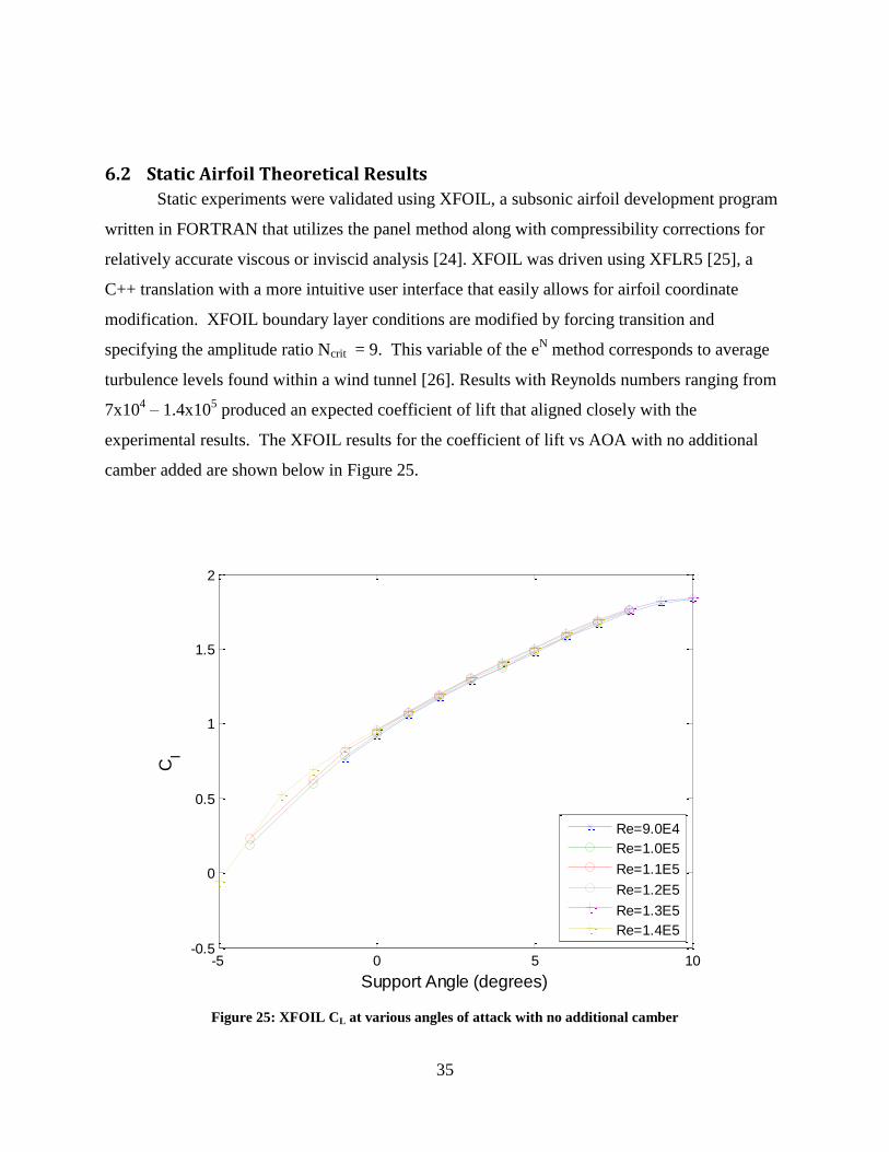
6.2 Static Airfoil Theoretical Results

Static experiments were validated using XFOIL, a subsonic airfoil development program

written in FORTRAN that utilizes the panel method along with compressibility corrections for

relatively accurate viscous or inviscid analysis [24]. XFOIL was driven using XFLR5 [25], a

C++ translation with a more intuitive user interface that easily allows for airfoil coordinate

modification. XFOIL boundary layer conditions are modified by forcing transition and

specifying the amplitude ratio Ncrit = 9. This variable of the eN method corresponds to average

turbulence levels found within a wind tunnel [26]. Results with Reynolds numbers ranging from

7x104 – 1.4x10

5 produced an expected coefficient of lift that aligned closely with the

experimental results. The XFOIL results for the coefficient of lift vs AOA with no additional

camber added are shown below in Figure 25.

Figure 25: XFOIL CL at various angles of attack with no additional camber

-5 0 5 10-0.5

0

0.5

1

1.5

2

Support Angle (degrees)

Cl

Re=9.0E4

Re=1.0E5

Re=1.1E5

Re=1.2E5

Re=1.3E5

Re=1.4E5

36

The AOA of zero degrees shown above is used for comparison to the unactuated airfoil

with a support angle of zero degrees. XFOIL suggests the coefficient of lift will be

approximately 0.9 for the airfoil at this AOA which is slightly higher than the average coefficient

of lift measured in the experimental results. Theoretical unactuated coefficients of lift for the

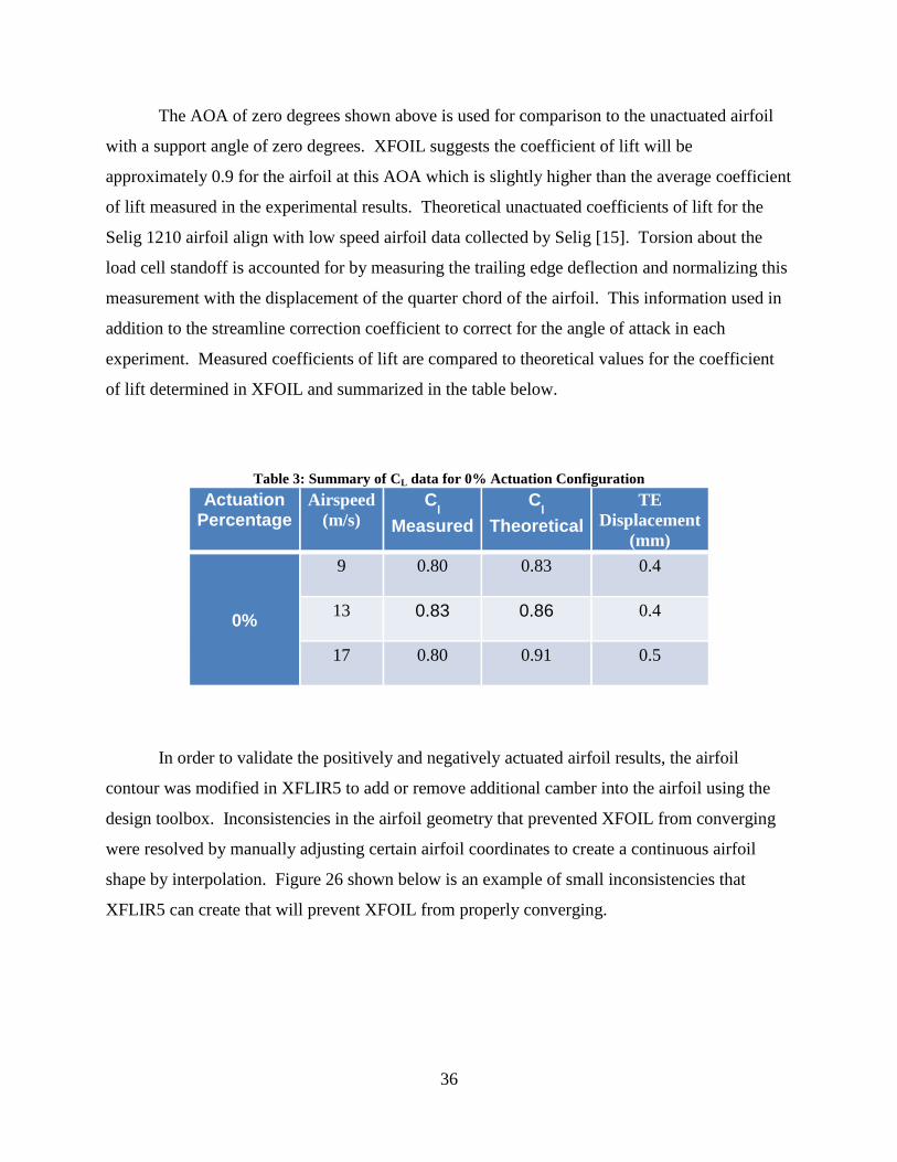
Selig 1210 airfoil align with low speed airfoil data collected by Selig [15]. Torsion about the

load cell standoff is accounted for by measuring the trailing edge deflection and normalizing this

measurement with the displacement of the quarter chord of the airfoil. This information used in

addition to the streamline correction coefficient to correct for the angle of attack in each

experiment. Measured coefficients of lift are compared to theoretical values for the coefficient

of lift determined in XFOIL and summarized in the table below.

Table 3: Summary of CL data for 0% Actuation Configuration

Actuation Percentage

Airspeed

(m/s) C

l

Measured

Cl

Theoretical

TE

Displacement (mm)

0%

9 0.80 0.83 0.4

13 0.83 0.86 0.4

17 0.80 0.91 0.5

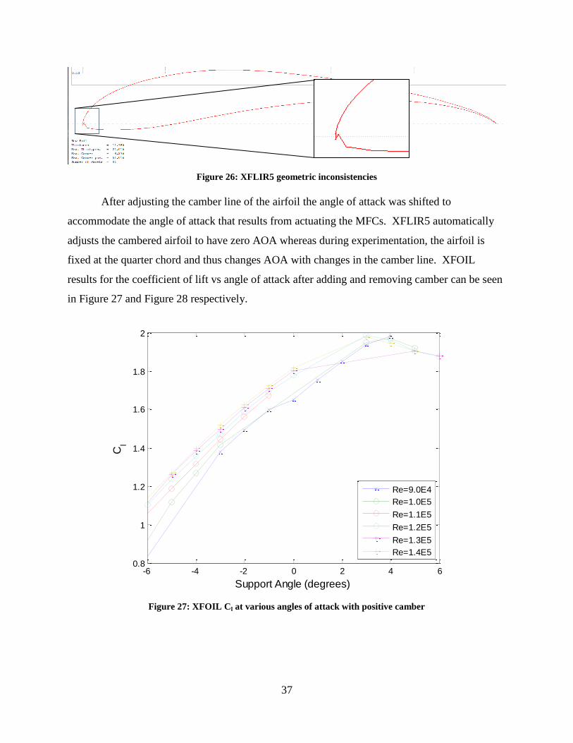
In order to validate the positively and negatively actuated airfoil results, the airfoil

contour was modified in XFLIR5 to add or remove additional camber into the airfoil using the

design toolbox. Inconsistencies in the airfoil geometry that prevented XFOIL from converging

were resolved by manually adjusting certain airfoil coordinates to create a continuous airfoil

shape by interpolation. Figure 26 shown below is an example of small inconsistencies that

XFLIR5 can create that will prevent XFOIL from properly converging.

37

Figure 26: XFLIR5 geometric inconsistencies

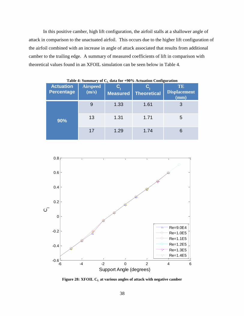
After adjusting the camber line of the airfoil the angle of attack was shifted to

accommodate the angle of attack that results from actuating the MFCs. XFLIR5 automatically

adjusts the cambered airfoil to have zero AOA whereas during experimentation, the airfoil is

fixed at the quarter chord and thus changes AOA with changes in the camber line. XFOIL

results for the coefficient of lift vs angle of attack after adding and removing camber can be seen

in Figure 27 and Figure 28 respectively.

Figure 27: XFOIL Cl at various angles of attack with positive camber

-6 -4 -2 0 2 4 60.8

1

1.2

1.4

1.6

1.8

2

Support Angle (degrees)

Cl

Re=9.0E4

Re=1.0E5

Re=1.1E5

Re=1.2E5

Re=1.3E5

Re=1.4E5

38

In this positive camber, high lift configuration, the airfoil stalls at a shallower angle of

attack in comparison to the unactuated airfoil. This occurs due to the higher lift configuration of

the airfoil combined with an increase in angle of attack associated that results from additional

camber to the trailing edge. A summary of measured coefficients of lift in comparison with

theoretical values found in an XFOIL simulation can be seen below in Table 4.

Table 4: Summary of CL data for +90% Actuation Configuration

Actuation Percentage

Airspeed

(m/s) C

l

Measured

Cl

Theoretical

TE

Displacement

(mm)

90%

9 1.33 1.61 3

13 1.31 1.71 5

17 1.29 1.74 6

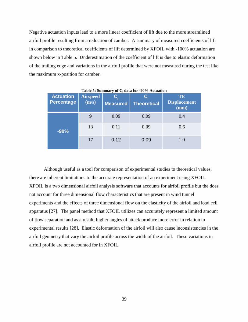
Figure 28: XFOIL CL at various angles of attack with negative camber

-6 -4 -2 0 2 4 6-0.6

-0.4

-0.2

0

0.2

0.4

0.6

0.8

Support Angle (degrees)

Cl

Re=9.0E4

Re=1.0E5

Re=1.1E5

Re=1.2E5

Re=1.3E5

Re=1.4E5

39

Negative actuation inputs lead to a more linear coefficient of lift due to the more streamlined

airfoil profile resulting from a reduction of camber. A summary of measured coefficients of lift

in comparison to theoretical coefficients of lift determined by XFOIL with -100% actuation are

shown below in Table 5. Underestimation of the coefficient of lift is due to elastic deformation

of the trailing edge and variations in the airfoil profile that were not measured during the test like

the maximum x-position for camber.

Table 5: Summary of Cl data for -90% Actuation

Actuation Percentage

Airspeed

(m/s) C

l

Measured

Cl

Theoretical

TE

Displacement

(mm)

-90%

9 0.09 0.09 0.4

13 0.11 0.09 0.6

17 0.12 0.09 1.0

Although useful as a tool for comparison of experimental studies to theoretical values,

there are inherent limitations to the accurate representation of an experiment using XFOIL.

XFOIL is a two dimensional airfoil analysis software that accounts for airfoil profile but the does

not account for three dimensional flow characteristics that are present in wind tunnel

experiments and the effects of three dimensional flow on the elasticity of the airfoil and load cell

apparatus [27]. The panel method that XFOIL utilizes can accurately represent a limited amount

of flow separation and as a result, higher angles of attack produce more error in relation to

experimental results [28]. Elastic deformation of the airfoil will also cause inconsistencies in the

airfoil geometry that vary the airfoil profile across the width of the airfoil. These variations in

airfoil profile are not accounted for in XFOIL.

40

6.3 Dynamic Test Results

After measuring the effects of aerodynamic loading on the airfoil trailing edge deflection

the dynamic response of the airfoil to an oscillatory input was measured. The purpose of these

experiments was to measure the lift response to an oscillatory MFC input. After this information

is collected, the phase difference between the MFC actuation input and the resulting

displacement of the trailing edge as well as the phase difference from the MFC input signal to a

resulting lift response is determined. This information is critical for implementation of MFCs in

high speed control surface applications.

The frequencies selected for the MFC input signal reside between the resonances found in

chapter 3. These were selected in order to avoid the resonant peaks and prevent over-attenuation

of the trailing edge deflection due to bandwidth limitations of the drive circuitry. Control signals

scaled the MFC actuation amplitude to 90% for all tests. This amplitude was selected because

low actuation amplitude bandwidth data had already been measured in previous research. The

bandwidth of higher actuation percentages better describes the lift authority that this MFC airfoil

is capable of producing. Dynamic testing was conducted at the same airspeeds as the static

testing section for the purpose of comparison. Lift responses shown exclude the initial half

second of data collection to mitigate any transient effects of the MFCs beginning the oscillation

cycle. Transient responses typically died out within the first 0.10 seconds.

This section is segregated by airspeed. FRF information is discussed for each frequency

after the lift data and FFT are presented. All lift data sets were filtered using a second order

Butterworth filter with a 60 Hz cutoff frequency to remove noise. The FFT was computed from

the original unfiltered lift signal to preserve all frequency data. The lift data shown below in

Figure 29 was measured without any airspeed and used as a control to compare all airspeeds

tested. Note that this set of data is not actually lift but instead represents forces measured solely

due to the inertial oscillations of the airfoil trailing edge. Lift data was normalized by

subtracting the inertial response data from each of the lift data sets.

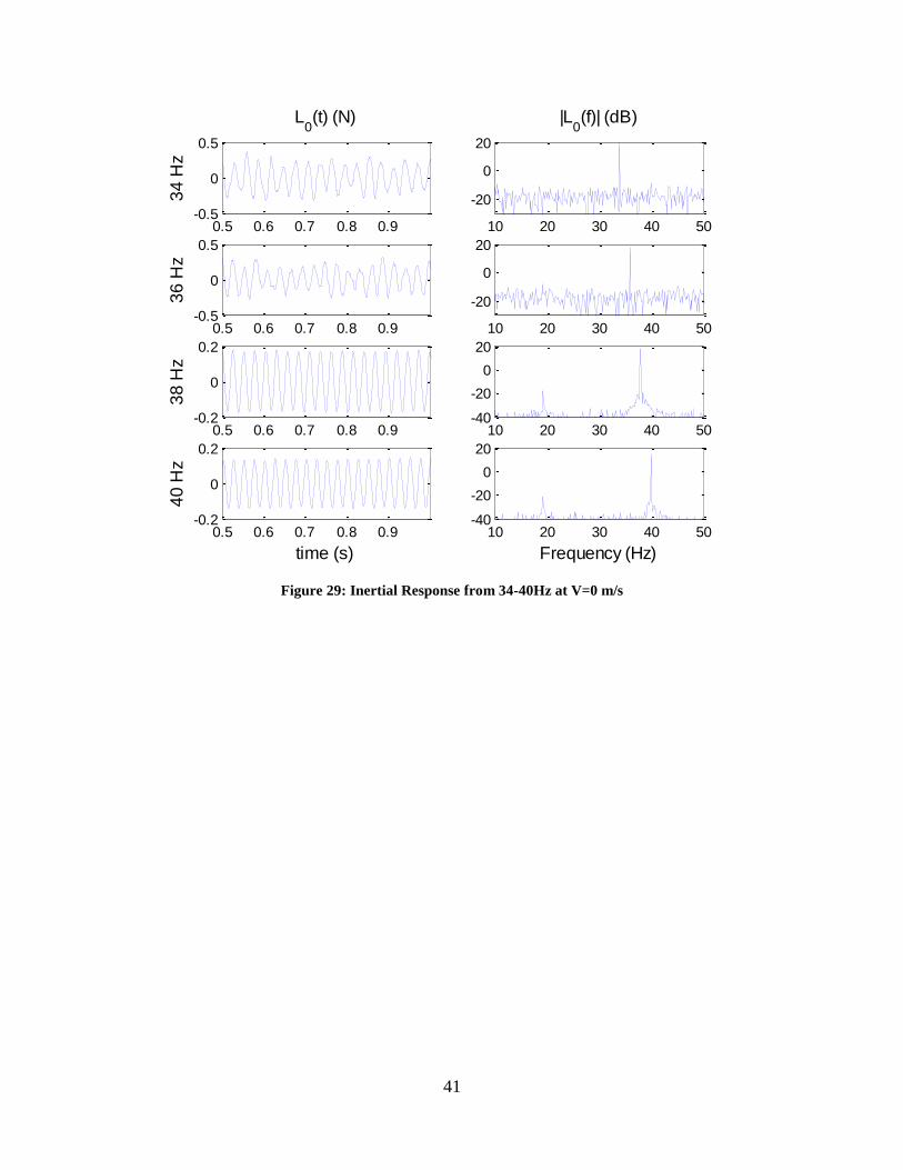
41

Figure 29: Inertial Response from 34-40Hz at V=0 m/s

0.5 0.6 0.7 0.8 0.9-0.5

0

0.5

34

Hz

L0(t) (N)

10 20 30 40 50

-20

0

20

|L0(f)| (dB)

0.5 0.6 0.7 0.8 0.9-0.5

0

0.5

36

Hz

10 20 30 40 50

-20

0

20

0.5 0.6 0.7 0.8 0.9-0.2

0

0.2

38

Hz

10 20 30 40 50-40

-20

0

20

0.5 0.6 0.7 0.8 0.9-0.2

0

0.2

time (s)

40

Hz

10 20 30 40 50-40

-20

0

20

Frequency (Hz)

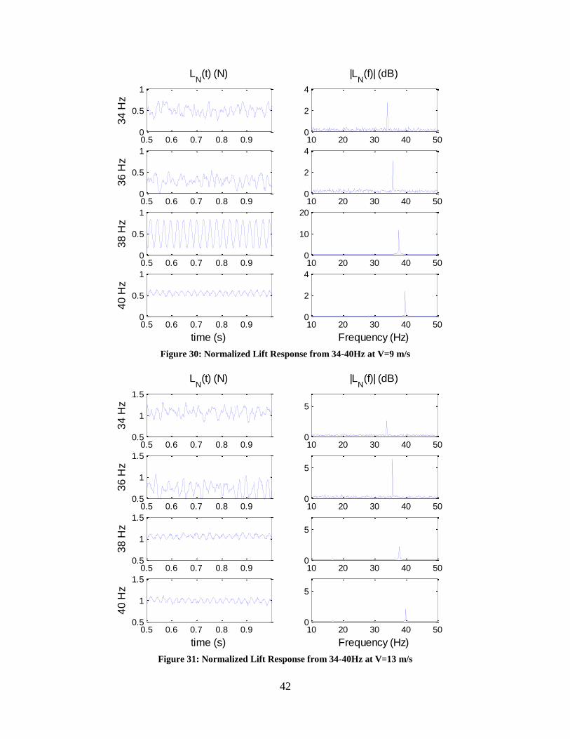
42

Figure 30: Normalized Lift Response from 34-40Hz at V=9 m/s

Figure 31: Normalized Lift Response from 34-40Hz at V=13 m/s

0.5 0.6 0.7 0.8 0.90

0.5

1

34

Hz

LN

(t) (N)

10 20 30 40 500

2

4

|LN

(f)| (dB)

0.5 0.6 0.7 0.8 0.90

0.5

1

36

Hz

10 20 30 40 500

2

4

0.5 0.6 0.7 0.8 0.90

0.5

1

38

Hz

10 20 30 40 500

10

20

0.5 0.6 0.7 0.8 0.90

0.5

1

time (s)

40

Hz

10 20 30 40 500

2

4

Frequency (Hz)

0.5 0.6 0.7 0.8 0.90.5

1

1.5

34

Hz

LN

(t) (N)

10 20 30 40 500

5

|LN

(f)| (dB)

0.5 0.6 0.7 0.8 0.90.5

1

1.5

36

Hz

10 20 30 40 500

5

0.5 0.6 0.7 0.8 0.90.5

1

1.5

38

Hz

10 20 30 40 500

5

0.5 0.6 0.7 0.8 0.90.5

1

1.5

time (s)

40

Hz

10 20 30 40 500

5

Frequency (Hz)

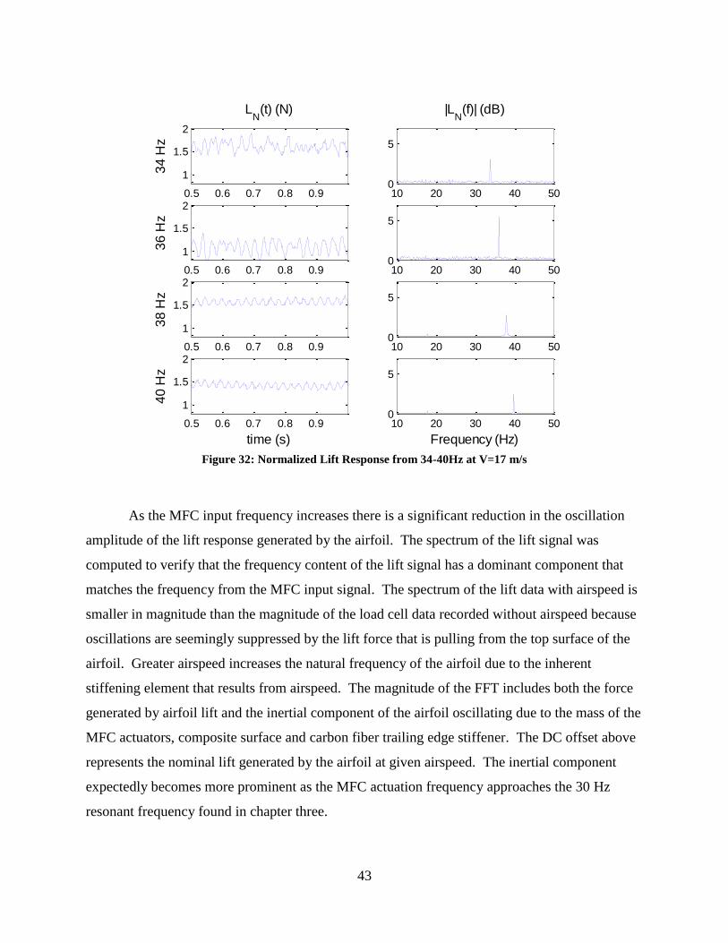
43

Figure 32: Normalized Lift Response from 34-40Hz at V=17 m/s

As the MFC input frequency increases there is a significant reduction in the oscillation

amplitude of the lift response generated by the airfoil. The spectrum of the lift signal was

computed to verify that the frequency content of the lift signal has a dominant component that

matches the frequency from the MFC input signal. The spectrum of the lift data with airspeed is

smaller in magnitude than the magnitude of the load cell data recorded without airspeed because

oscillations are seemingly suppressed by the lift force that is pulling from the top surface of the

airfoil. Greater airspeed increases the natural frequency of the airfoil due to the inherent

stiffening element that results from airspeed. The magnitude of the FFT includes both the force

generated by airfoil lift and the inertial component of the airfoil oscillating due to the mass of the

MFC actuators, composite surface and carbon fiber trailing edge stiffener. The DC offset above

represents the nominal lift generated by the airfoil at given airspeed. The inertial component

expectedly becomes more prominent as the MFC actuation frequency approaches the 30 Hz

resonant frequency found in chapter three.

0.5 0.6 0.7 0.8 0.9

1

1.5

2

34

Hz

LN

(t) (N)

10 20 30 40 500

5

|LN

(f)| (dB)

0.5 0.6 0.7 0.8 0.9

1

1.5

2

36

Hz

10 20 30 40 500

5

0.5 0.6 0.7 0.8 0.9

1

1.5

2

38

Hz

10 20 30 40 500

5

0.5 0.6 0.7 0.8 0.9

1

1.5

2

time (s)

40

Hz

10 20 30 40 500

5

Frequency (Hz)

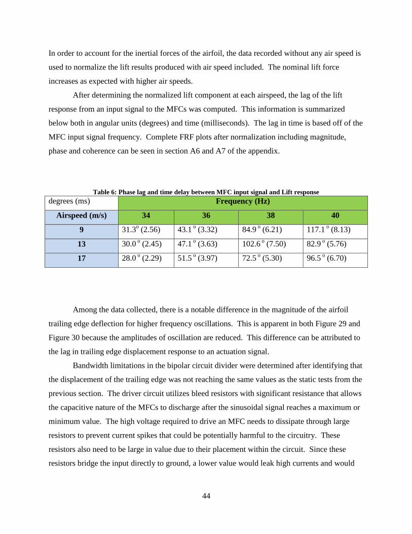
44

In order to account for the inertial forces of the airfoil, the data recorded without any air speed is

used to normalize the lift results produced with air speed included. The nominal lift force

increases as expected with higher air speeds.

After determining the normalized lift component at each airspeed, the lag of the lift

response from an input signal to the MFCs was computed. This information is summarized

below both in angular units (degrees) and time (milliseconds). The lag in time is based off of the

MFC input signal frequency. Complete FRF plots after normalization including magnitude,

phase and coherence can be seen in section A6 and A7 of the appendix.

Table 6: Phase lag and time delay between MFC input signal and Lift response

degrees (ms) Frequency (Hz)

Airspeed (m/s) 34 36 38 40

9 31.3o (2.56) 43.1

o (3.32) 84.9

o (6.21) 117.1

o (8.13)

13 30.0 o (2.45) 47.1

o (3.63) 102.6

o (7.50) 82.9

o (5.76)

17 28.0 o (2.29) 51.5

o (3.97) 72.5

o (5.30) 96.5

o (6.70)

Among the data collected, there is a notable difference in the magnitude of the airfoil

trailing edge deflection for higher frequency oscillations. This is apparent in both Figure 29 and

Figure 30 because the amplitudes of oscillation are reduced. This difference can be attributed to

the lag in trailing edge displacement response to an actuation signal.

Bandwidth limitations in the bipolar circuit divider were determined after identifying that

the displacement of the trailing edge was not reaching the same values as the static tests from the

previous section. The driver circuit utilizes bleed resistors with significant resistance that allows

the capacitive nature of the MFCs to discharge after the sinusoidal signal reaches a maximum or

minimum value. The high voltage required to drive an MFC needs to dissipate through large

resistors to prevent current spikes that could be potentially harmful to the circuitry. These

resistors also need to be large in value due to their placement within the circuit. Since these

resistors bridge the input directly to ground, a lower value would leak high currents and would

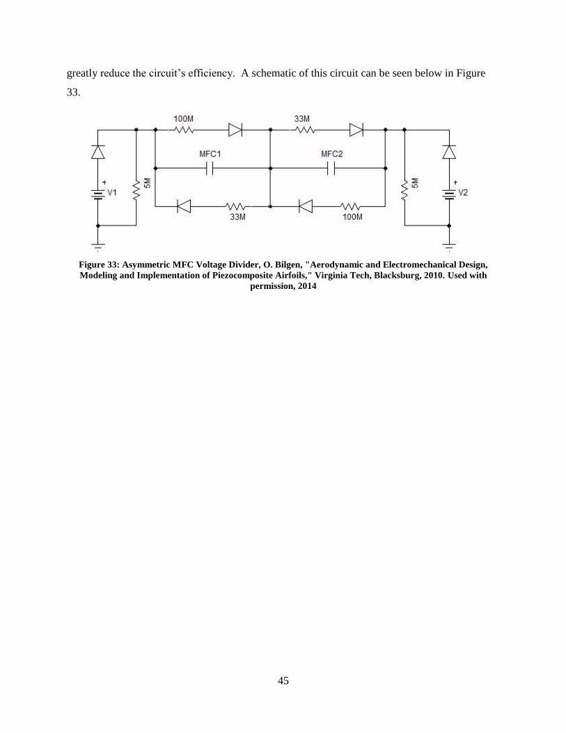
45

greatly reduce the circuit’s efficiency. A schematic of this circuit can be seen below in Figure

33.

Figure 33: Asymmetric MFC Voltage Divider, O. Bilgen, "Aerodynamic and Electromechanical Design,

Modeling and Implementation of Piezocomposite Airfoils," Virginia Tech, Blacksburg, 2010. Used with

permission, 2014

46

Chapter 7

7 Airfoil Surface Model

This chapter explains how airfoil surface displacements measured during dynamic wind

tunnel testing can be used to generate a cost effective empirical model of the airfoil surface

contour. This could potentially be used for validating parametric models and to improve the

accuracy of the geometric models used in vortex lattice simulations by including small dynamic

surface deformations that are otherwise assumed to be nonexistent.

7.1 Surface Modeling Method and Assumptions

Surface displacement data is used to generate a 2D model of changes in airfoil contour

during a wind tunnel test. Unactuated coordinates for the upper and lower airfoil surfaces were

obtained from the UIUC Applied Aerodynamics Airfoil Coordinate Database [29]. In order to

create the initial surface model, the airfoil was broken up between the upper MFC surface aft of

the D-box, the lower wiper surface, and the leading edge D-box itself. Since the leading edge is

constructed from basswood, it was assumed to be rigid for this model and only rigid body

translation and pitch were considered for this section of the airfoil.

In order to model the fiberglass/MFC surface of the airfoil, the surface displacements were

measured at various points along the airfoil span using a laser displacement sensor during

oscillatory experiments. Potential phase differences in each experiment were accounted for by

utilizing the MFC input signal as a clock reference. Data sets were shifted so that the phase of

the MFC input signal from each experiment was aligned. Displacement data was smoothed

using a fourth order low pass Butterworth filter with a 60 Hz cutoff frequency. The profile of the

trailing edge MFC surface was created using a third order polynomial fit for each set of recorded

displacement data. This polynomial is reconstructed for each data set to reflect the current

profile of the airfoil at each sample instance. A third order polynomial was selected as a

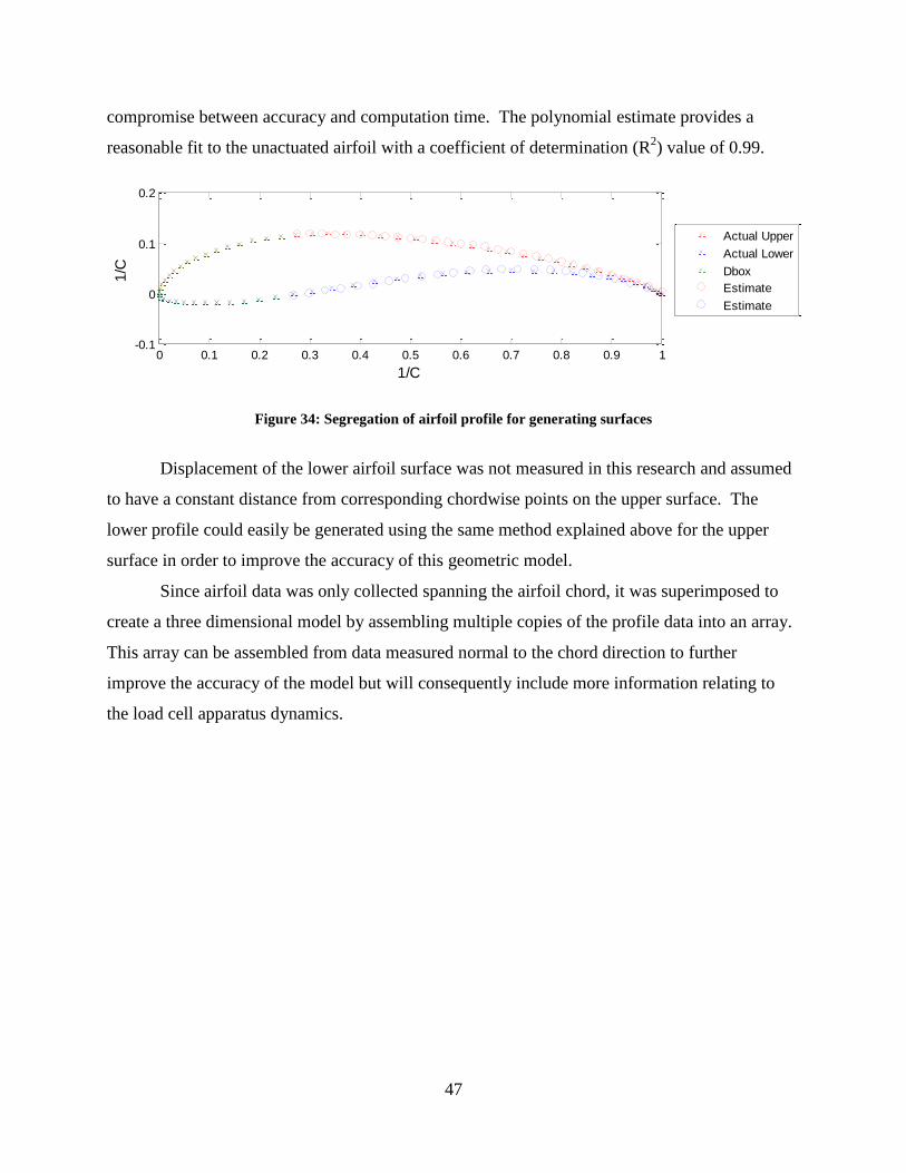
47

compromise between accuracy and computation time. The polynomial estimate provides a

reasonable fit to the unactuated airfoil with a coefficient of determination (R2) value of 0.99.

Figure 34: Segregation of airfoil profile for generating surfaces

Displacement of the lower airfoil surface was not measured in this research and assumed

to have a constant distance from corresponding chordwise points on the upper surface. The

lower profile could easily be generated using the same method explained above for the upper

surface in order to improve the accuracy of this geometric model.

Since airfoil data was only collected spanning the airfoil chord, it was superimposed to

create a three dimensional model by assembling multiple copies of the profile data into an array.

This array can be assembled from data measured normal to the chord direction to further

improve the accuracy of the model but will consequently include more information relating to

the load cell apparatus dynamics.

0 0.1 0.2 0.3 0.4 0.5 0.6 0.7 0.8 0.9 1-0.1

0

0.1

0.2

1/C

1/C

Actual Upper

Actual Lower

Dbox

Estimate

Estimate

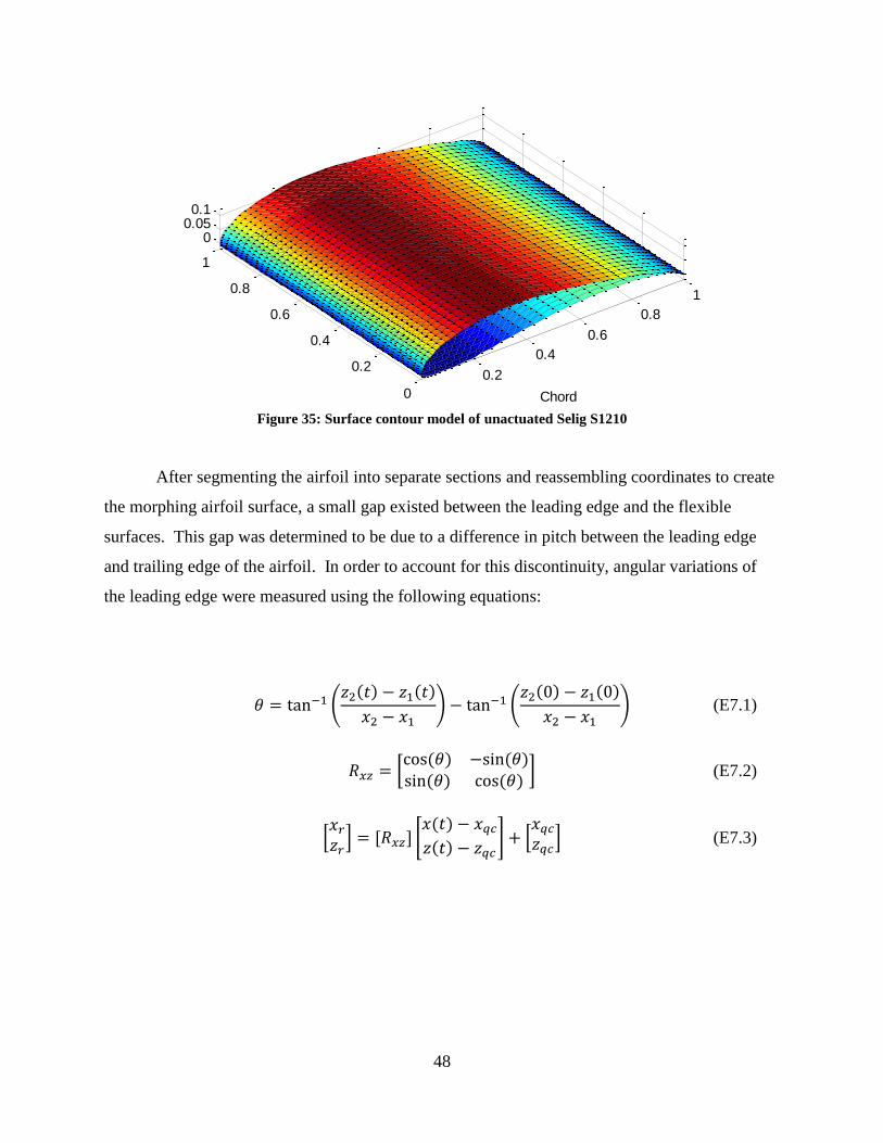
48

Figure 35: Surface contour model of unactuated Selig S1210

After segmenting the airfoil into separate sections and reassembling coordinates to create

the morphing airfoil surface, a small gap existed between the leading edge and the flexible

surfaces. This gap was determined to be due to a difference in pitch between the leading edge

and trailing edge of the airfoil. In order to account for this discontinuity, angular variations of

the leading edge were measured using the following equations:

𝜃 = tan−1 (𝑧2(𝑡) − 𝑧1(𝑡)

𝑥2 − 𝑥1) − tan−1 (

𝑧2(0) − 𝑧1(0)

𝑥2 − 𝑥1) (E7.1)

𝑅𝑥𝑧 = [cos(𝜃) −sin(𝜃)sin(𝜃) cos(𝜃)

] (E7.2)

[𝑥𝑟𝑧𝑟] = [𝑅𝑥𝑧] [

𝑥(𝑡) − 𝑥𝑞𝑐𝑧(𝑡) − 𝑧𝑞𝑐

] + [𝑥𝑞𝑐𝑧𝑞𝑐

] (E7.3)

0.2

0.4

0.6

0.8

1

0

0.2

0.4

0.6

0.8

1

00.050.1

Chord

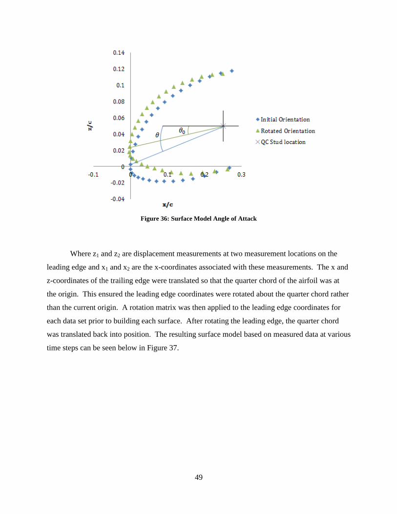
49

Figure 36: Surface Model Angle of Attack

Where z1 and z2 are displacement measurements at two measurement locations on the

leading edge and x1 and x2 are the x-coordinates associated with these measurements. The x and

z-coordinates of the trailing edge were translated so that the quarter chord of the airfoil was at

the origin. This ensured the leading edge coordinates were rotated about the quarter chord rather

than the current origin. A rotation matrix was then applied to the leading edge coordinates for

each data set prior to building each surface. After rotating the leading edge, the quarter chord

was translated back into position. The resulting surface model based on measured data at various

time steps can be seen below in Figure 37.

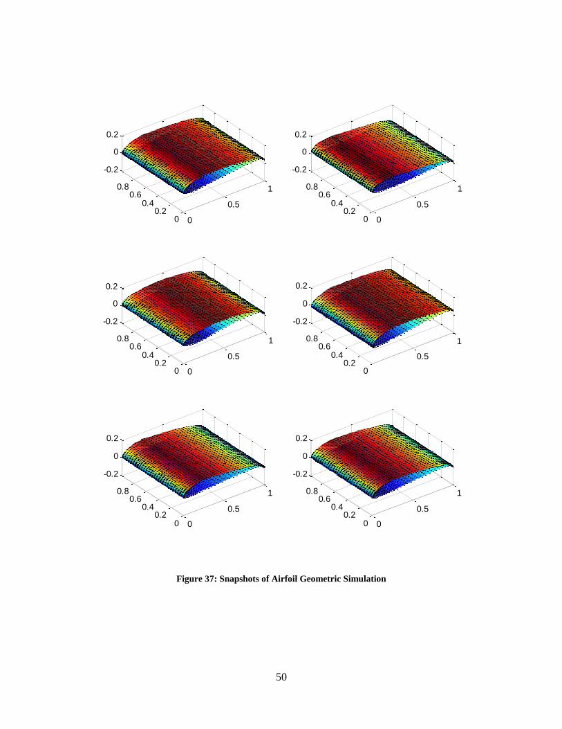
50

Figure 37: Snapshots of Airfoil Geometric Simulation

0

0.5

1

00.2

0.40.6

0.8

-0.2

0

0.2

0

0.5

1

00.2

0.40.6

0.8

-0.2

0

0.2

0

0.5

1

00.2

0.40.6

0.8

-0.2

0

0.2

0.5

1

00.2

0.40.6

0.8

-0.2

0

0.2

0

0.5

1

00.2

0.40.6

0.8

-0.2

0

0.2

0

0.5

1

00.2

0.40.6

0.8

-0.2

0

0.2

51

Chapter 8

8 Conclusion

8.1 Summary

This research presents experimental results of oscillatory lift generated using MFC

morphing airfoils for the purpose of evaluating the use of Macro-Fiber Composites as an

oscillatory lift control mechanism. Modal analysis of the airfoil and load cell structure

highlighted resonant frequencies and mode shapes of the airfoil. This provided insight as to what

vibratory phenomena is to be expected during wind tunnel testing due to the load cell and airfoil

structure. The effect of aerodynamic loading on trailing edge deflection with high MFC

actuation percentages and without actuation was measured at various airspeeds. Flutter

characteristics from aerodynamic loading were analyzed and the magnitudes of oscillation were

shown to vary significantly with airspeed. Deviations in the coefficient of lift from expected

values due to aerodynamic loading were measured up to 17 m/s.

Bandwidth limitations of the current amplifier, driver circuitry, and MFC structure were

discovered and shown to have a significant impact on the resulting amplitude of a bimorph MFC

configuration. Transfer functions between the input signal and lift response are used to account

for inertial forces generated by the oscillating airfoil and to extract magnitude and phase

information at various airspeeds and input frequencies. Lag in the lift response from the MFC

input signal was recorded at various air speeds and actuation frequencies for high actuation

inputs. Airfoil surface displacement was measured at various points on the airfoil during

oscillatory testing and used to create a geometric model of changes in the airfoil contour during

wind tunnel testing.

The bandwidth performance of MFCs as an oscillatory lift mechanism is limited by both

the structure that the MFCs are bonded to and the amplifier/divider circuitry used to supply the

high voltage requirements. Aerodynamic and mechanical systems utilizing this technology as an

actuator would benefit from feedback control to compensate for both hysteresis and aerodynamic

loading.

52

8.2 Recommendations for Future Work

This research focused on analyzing experimental results of oscillatory lift in a specific

airfoil configuration with one type of MFC. There is still work to be done in determining

characteristics of a broader selection of these actuators. The relatively low cost of these

actuators has given way to custom MFC configurations that can be made to order [1].

Comparison of the performance characteristics with custom MFC shapes versus the standard

actuator footprint is not yet documented. Experimentation on the effects of laminate adhesives

on the performance characteristics of MFCs would be another interesting analysis that could help

characterize the effects of different bonding agents. Testing of symmetric airfoils with MFCs on

the upper and lower surface could provide more actuator authority in aerodynamic applications.

The ability to morph a symmetric airfoil to produce an asymmetric contour in either direction

could benefit UAVs that fly inverted often.

Computational fluid dynamics simulations and smoke wire visualization of MFCs would

help to further characterization of limit cycle oscillations that are a trending phenomenon in

MFC wind tunnel testing. Effects on of oscillating camber on vortex formation could shed light

on optimum oscillatory frequencies for specific airfoil shapes. Investigation of leading edge and

trailing edge vortices could provide more insight into aerodynamic coupling between the

structure and wake. Active control to dampen limit cycle oscillations would also make for

another exciting research topic. This investigation into higher harmonic control is currently

being studied by many other researchers.

The wind tunnel could be updated to include a measurement system for the airfoil pitching

moment that results from a varying center of pressure when the airfoil morphs. This

measurement system would provide more detailed expectations for resulting pitch when MFC

control surfaces are actuated.

53

Bibliography

[1] "smart-materials.com," Smart Material, [Online]. Available: http://www.smart-

material.com/MFC-product-main.html. [Accessed 2014].

[2] W. Wilkie, D. Inman, J. High and R. B. Willams, "Recent Developments in NASA

Piezocomposite Actuator Technology," in 9th International Conference on New Actuators;

14-15 Jun. 2004; Breman; Germany, 2004.

[3] O. Bilgen, "Aerodynamic and Electromechanical Design, Modeling and Implementation of

Piezocomposite Airfoils," Virginia Tech, Blacksburg, 2010.

[4] E. Gustafson, "Design, Simulation, and Wind Tunnel Verification of a Morphing Airfoil,"

Virginia Tech, Blacksburg, Va, 2011.

[5] T. Probst, "Evaluating the Aerodynamic Performance of MFC-Actuated Morphing Wings to

Control a Small UAV," Virginia Tech, Blacksburg, VA, 2012.

[6] D.-K. Kim and J.-H. Han, "Smart Flapping Wing Using Macro-Fiber Composite Actuators,"

SPIE 13th Annual Symposium Smart Structures and Materials, 2006.

[7] R. Duffy, J. Dubben, J. Nickerson and J. Colasante, "A Theoretical and Experimental Study

of the Snap-Through Airfoil and its Potential as a Higher Harmonic Control Device," AIAA

26th Aerospace Sciences Meeting, no. AA-88-0668, 1988.

[8] N. Pern and J. Jacob, "Wake Vortex Mitigation Using Adaptive Airfoils: The Piezoelectric

Arc Airfoil," 37th AIAA Aerospace Sciences Meeting and Exhibit, no. 99-0524, 1999.

[9] D. Munday and J. Jacob, "Active Control of Separation on Wing with Oscillating Camber,"

AIAA Aerospace Sciences Meeting and Exhibit, no. AIAA-2001-0293, 2001.

[10] J. Clement, "Bench-Top Characterization of an Active Rotor Blade Flap System

Incorporating C-Block Actuators," AIAA, vol. 98, pp. 2857-2869, 1998.

[11] J. Garcia, "Active Helicopter Rotor Control Using Blade-Mounted Actuators,"

Massachusetts Institute of Technology, Cambridge, 1994.

[12] F. Straub and D. Merkley, "Design of a Smart Material Actuator for Rotor Control," Smart

Material Structures, pp. 223-234, 1997.

[13] T. Mueller, "Aerodynamic Measurements at Low Reynolds Numbers for Fixed Wing

Micro-Air Vehicles," Department of Aerospace and Mechanical Engineering, University of

Notre Dame, Notre Dame, IN, 1999.

[14] R. W. a. P. A. Barlow J.B., Low-Speed Wind Tunnel Testing, John Wiley and Sons 3rd ed.,

1999.

[15] M. a. G. J. a. B. A. a. G. P. Selig, "Summary of Low-Speed Airfoil Data," SolarTech

Publications, Virginia Beach, 1995.

[16] "Clarkson University," [Online]. Available:

http://people.clarkson.edu/~pmarzocc/AE429/AE-429-4.pdf. [Accessed September 2014].

[17] O. J. Ohanian, "Piezoelectric Composite Morphing Control Surfaces for Unmanned Aerial

54

Vehicles," Sensors and Smart Structures Technologies for Civil, Mechanical, and

Aerospace Systems, vol. 7981, 2011.

[18] S.-W. L. T.-Y. W. T.-J. Yeh, "Modeling and Identification of Hysteresis in Piezoelectric

Actuators," Journal of Dynamic Systems, Measurement, and Control, vol. 128, June 2006.

[19] Noliac, "www.noliac.com'Material_characteristics," 2011. [Online]. Available:

http://www.noliac.com/Material_characteristics_-143.aspx. [Accessed 20 July 2014].

[20] J. H. Schafer J, "Compensation of Hysteresis in Solid-State Actuators," Sensors and

Actuators, pp. 97-102, 1995.

[21] H. J. K. Kuhnen, "Compensation of the Creep and Hysteresis Effects of Piezoelectric

Actuators with Inverse Systems," University of Saarland, Saarbrucken, Germany.

[22] C. Visone, "Hysteresis Modelling and Compensation for Smart Sensors and Actuators,"

International Workshop on Multi-Rate Processes and Hysteresis; Journal of Physics:

Conference Series 138, vol. 138, 2008.

[23] P. Mayuresh, "Limit Cycle Oscillations of Aircraft due to Flutter-Induced Drag," AIAA

Structures, Structural Dynamics, and Materials Conference, vol. 43, 2002.

[24] M. a. Y. H. Drela, "XFOIL Subsonic Airfoil Development System (Version 6.99)," MIT,

Dec 2013. [Online]. Available: http://web.mit.edu/drela/Public/web/xfoil/. [Accessed 29

August 2014].

[25] "xflr5.com," 1 February 2014. [Online]. Available:

http://www.xflr5.com/ReleaseNotes.htm. [Accessed June 2014].

[26] M. Drela, "XFOIL Subsonic Airfoil Develpment System," [Online]. Available:

http://web.mit.edu/drela/Public/web/xfoil/. [Accessed September 2014].

[27] D. Boon, "Application of Uncertainty Quantification to a Fluid-Structure Interaction

Experiment - Providing Accurate Insight in Uncertain Phenomena," Delft University of

Technology, Netherlands, 2011.

[28] T. Speer, "Aerodynamics Of Teardrop Wingmasts," Des Moines, Washington.

[29] U. A. A. G. -. D. o. A. Engineering, "UIUC Airfoil Coordinates Database," [Online].

Available: http://aerospace.illinois.edu/m-selig/ads/coord_database.html. [Accessed 12 03

2014].

[30] P. Cantrell, "The Helicopter Aviation Home Page," [Online]. Available:

http://www.copters.com/helicopter.html. [Accessed 27 April 2014].

[31] P. Ge and M. Jouaneh, "Tracking Control of a Piezoceramic Actuator," IEEE Trans on

Control sys. Tech., pp. 209-216, 1996.

[32] G. D. a. D. Balmford, Bramwell's Helicopter Dynamics Second Edition, A.R.S. Bramwell

and AIAA, 2001.

[33] L. T. G. S. G. T. T. N. Burner A.W., "Aeroelastic Deformation Measurements of Flap, Gap,

and Overhang on a Semispan Model," Journal of Aircraft, vol. 38, no. 6, pp. 1147-1154,

2001.

[34] R. Bielawa, Rotary Wing Structural Dynamics and Aeroelasticity, Salem: American

Institute of Aeronautics and Astronautics, 1992.

[35] M. a. W. K. Wilber, "Active-Twist Rotor Control Applications for UAVs," nasa.gov, 2004.

[36] J. Pope A. and Harper, Low Speed Wind Tunnel Testing, New York: Wiley and Sons, 1966.

55

[37] I. Ross, "Wind Tunnel Blockage Corrections: An Application to Vertical-Axis Wind

Turbines," University of Dayton, Dayton, Ohio, 2012.

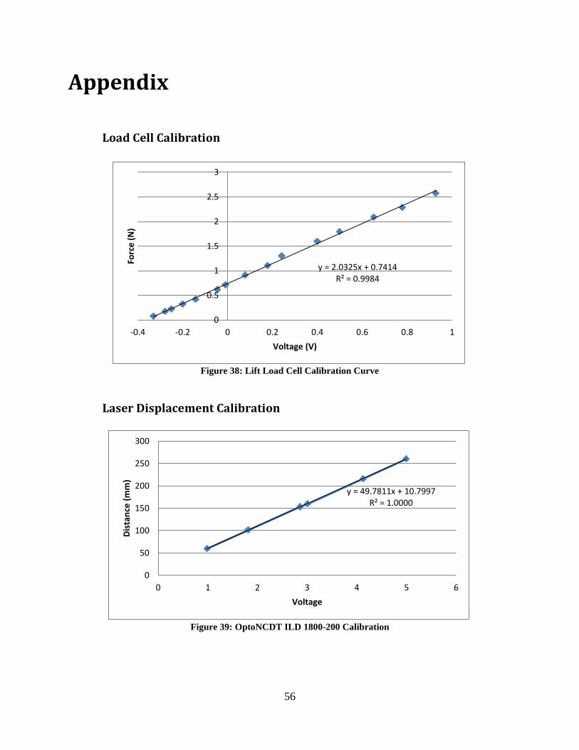
56

Appendix

Load Cell Calibration

Figure 38: Lift Load Cell Calibration Curve

Laser Displacement Calibration

Figure 39: OptoNCDT ILD 1800-200 Calibration

y = 2.0325x + 0.7414 R² = 0.9984

0

0.5

1

1.5

2

2.5

3

-0.4 -0.2 0 0.2 0.4 0.6 0.8 1

Forc

e (

N)

Voltage (V)

y = 49.7811x + 10.7997 R² = 1.0000

0

50

100

150

200

250

300

0 1 2 3 4 5 6

Dis

tan

ce (

mm

)

Voltage

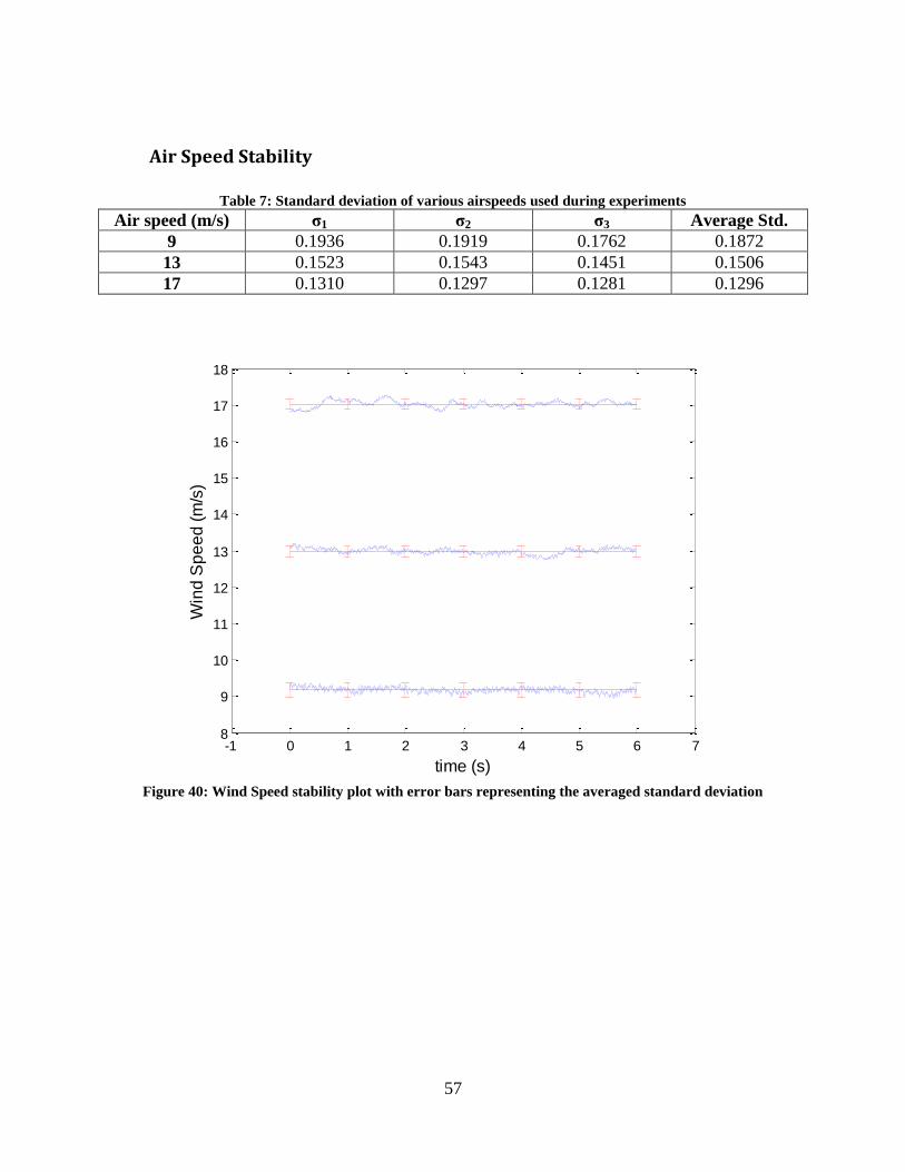
57

Air Speed Stability

Table 7: Standard deviation of various airspeeds used during experiments

Air speed (m/s) σ1 σ2 σ3 Average Std.

9 0.1936 0.1919 0.1762 0.1872

13 0.1523 0.1543 0.1451 0.1506

17 0.1310 0.1297 0.1281 0.1296

Figure 40: Wind Speed stability plot with error bars representing the averaged standard deviation

-1 0 1 2 3 4 5 6 78

9

10

11

12

13

14

15

16

17

18

Win

d S

pe

ed

(m

/s)

time (s)

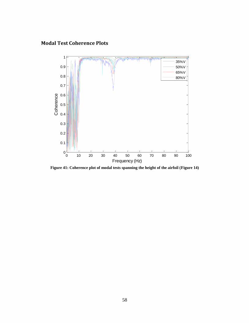
58

Modal Test Coherence Plots

Figure 41: Coherence plot of modal tests spanning the height of the airfoil (Figure 14)

0 10 20 30 40 50 60 70 80 90 1000

0.1

0.2

0.3

0.4

0.5

0.6

0.7

0.8

0.9

1

Frequency (Hz)

Co

he

ren

ce

35%V

50%V

65%V

80%V

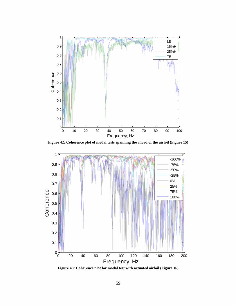
59

Figure 42: Coherence plot of modal tests spanning the chord of the airfoil (Figure 15)

Figure 43: Coherence plot for modal test with actuated airfoil (Figure 16)

0 10 20 30 40 50 60 70 80 90 1000

0.1

0.2

0.3

0.4

0.5

0.6

0.7

0.8

0.9

1

Frequency, Hz

Co

he

ren

ce

LE

15%H

25%H

TE

0 20 40 60 80 100 120 140 160 180 2000

0.1

0.2

0.3

0.4

0.5

0.6

0.7

0.8

0.9

1

Frequency, Hz

Co

he

ren

ce

-100%

-75%

-50%

-25%

0%

25%

75%

100%

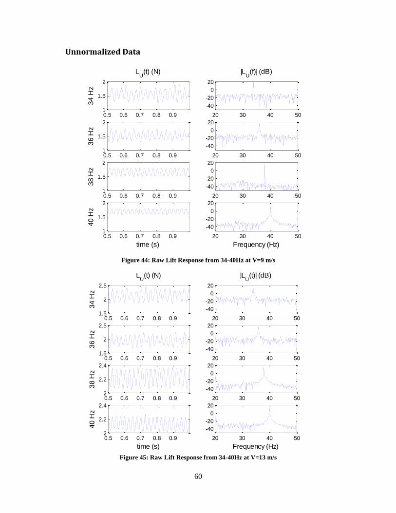
60

Unnormalized Data

Figure 44: Raw Lift Response from 34-40Hz at V=9 m/s

Figure 45: Raw Lift Response from 34-40Hz at V=13 m/s

0.5 0.6 0.7 0.8 0.91

1.5

2

34

Hz

LU

(t) (N)

20 30 40 50

-40

-20

0

20

|LU

(f)| (dB)

0.5 0.6 0.7 0.8 0.91

1.5

2

36

Hz

20 30 40 50

-40

-20

0

20

0.5 0.6 0.7 0.8 0.91

1.5

2

38

Hz

20 30 40 50

-40

-20

0

20

0.5 0.6 0.7 0.8 0.91

1.5

2

time (s)

40

Hz

20 30 40 50

-40

-20

0

20

Frequency (Hz)

0.5 0.6 0.7 0.8 0.91.5

2

2.5

34

Hz

LU

(t) (N)

20 30 40 50

-40

-20

0

20

|LU

(t)| (dB)

0.5 0.6 0.7 0.8 0.91.5

2

2.5

36

Hz

20 30 40 50

-40

-20

0

20

0.5 0.6 0.7 0.8 0.92

2.2

2.4

38

Hz

20 30 40 50

-40

-20

0

20

0.5 0.6 0.7 0.8 0.92

2.2

2.4

time (s)

40

Hz

20 30 40 50

-40

-20

0

20

Frequency (Hz)

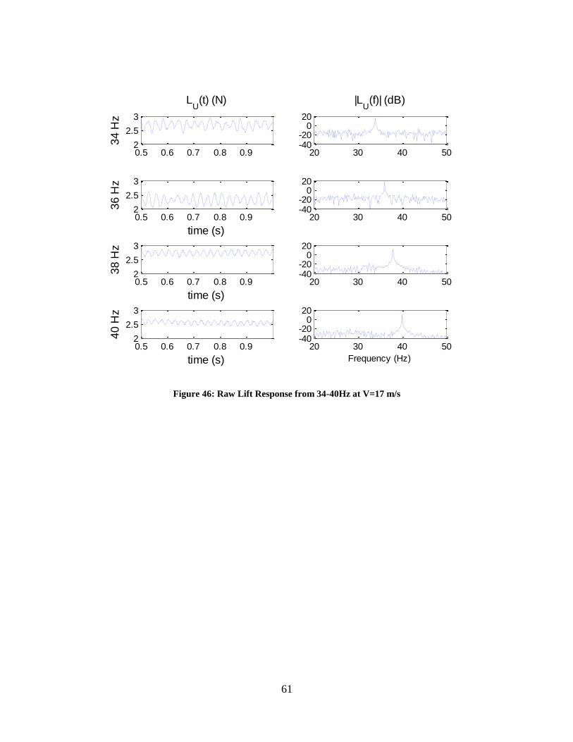
61

Figure 46: Raw Lift Response from 34-40Hz at V=17 m/s

0.5 0.6 0.7 0.8 0.92

2.5

33

4 H

z

LU

(t) (N)

20 30 40 50-40-20

020

|LU

(f)| (dB)

0.5 0.6 0.7 0.8 0.92

2.5

3

36

Hz

time (s)

20 30 40 50-40-20

020

0.5 0.6 0.7 0.8 0.92

2.5

3

time (s)

38

Hz

20 30 40 50-40-20

020

0.5 0.6 0.7 0.8 0.92

2.5

3

time (s)

40

Hz

20 30 40 50-40-20

020

Frequency (Hz)

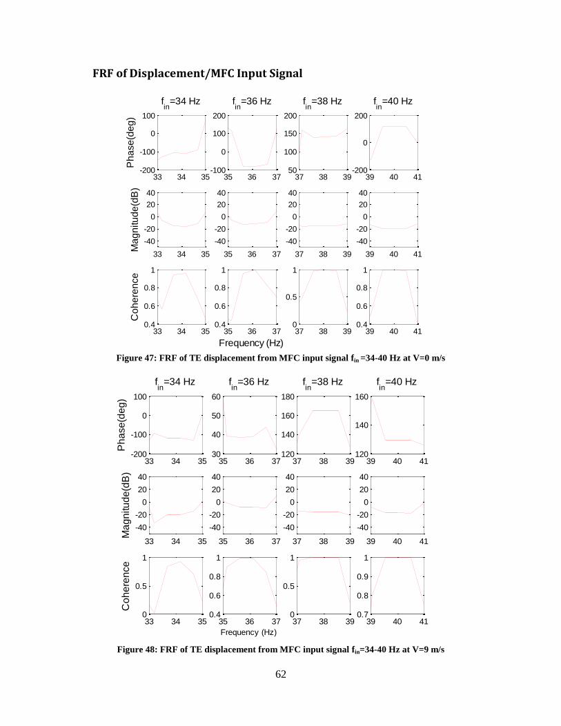
62

FRF of Displacement/MFC Input Signal

Figure 47: FRF of TE displacement from MFC input signal fin =34-40 Hz at V=0 m/s

Figure 48: FRF of TE displacement from MFC input signal fin=34-40 Hz at V=9 m/s

33 34 35

-40

-20

0

20

40

Ma

gn

itu

de

(dB

)

33 34 35-200

-100

0

100

Ph

ase

(de

g)

fin

=34 Hz

33 34 350.4

0.6

0.8

1

Co

he

ren

ce

35 36 370.4

0.6

0.8

1

Frequency (Hz)

35 36 37

-40

-20

0

20

40

35 36 37-100

0

100

200

fin

=36 Hz

37 38 390

0.5

1

37 38 39

-40

-20

0

20

40

37 38 3950

100

150

200

fin

=38 Hz

39 40 410.4

0.6

0.8

1

39 40 41

-40

-20

0

20

40

39 40 41-200

0

200

fin

=40 Hz

33 34 350

0.5

1

Co

he

ren

ce

33 34 35

-40

-20

0

20

40

Ma

gn

itu

de

(dB

)

33 34 35-200

-100

0

100

Ph

ase

(de

g)

fin

=34 Hz

35 36 370.4

0.6

0.8

1

Frequency (Hz)

35 36 37

-40

-20

0

20

40

35 36 3730

40

50

60

fin

=36 Hz

37 38 390

0.5

1

37 38 39

-40

-20

0

20

40

37 38 39120

140

160

180

fin

=38 Hz

39 40 410.7

0.8

0.9

1

39 40 41

-40

-20

0

20

40

39 40 41120

140

160

fin

=40 Hz

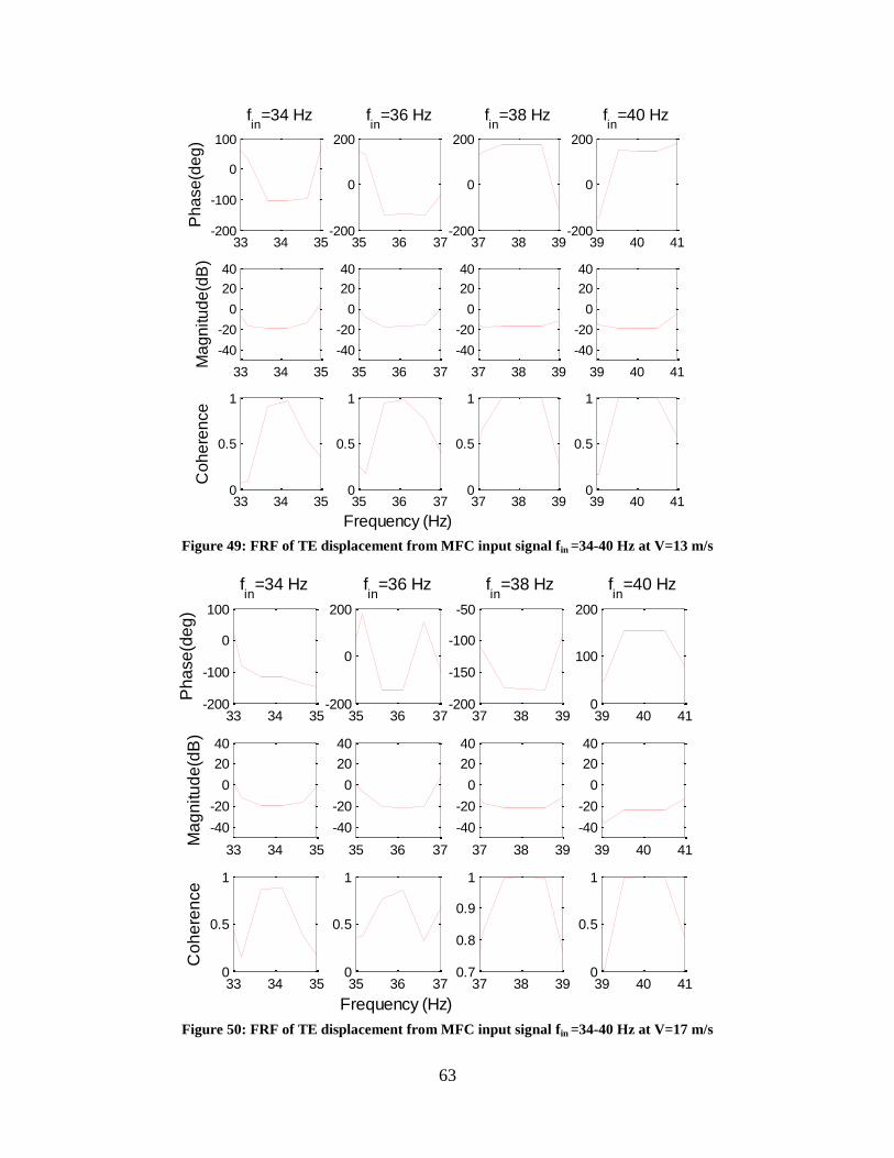
63

Figure 49: FRF of TE displacement from MFC input signal fin =34-40 Hz at V=13 m/s

Figure 50: FRF of TE displacement from MFC input signal fin =34-40 Hz at V=17 m/s

33 34 350

0.5

1

Co

he

ren

ce

33 34 35

-40

-20

0

20

40

Ma

gn

itu

de

(dB

)

33 34 35-200

-100

0

100

Ph

ase

(de

g)

fin

=34 Hz

35 36 370

0.5

1

Frequency (Hz)

35 36 37

-40

-20

0

20

40

35 36 37-200

0

200

fin

=36 Hz

37 38 390

0.5

1

37 38 39

-40

-20

0

20

40

37 38 39-200

0

200

fin

=38 Hz

39 40 410

0.5

1

39 40 41

-40

-20

0

20

40

39 40 41-200

0

200

fin

=40 Hz

33 34 350

0.5

1

Co

he

ren

ce

33 34 35

-40

-20

0

20

40

Ma

gn

itu

de

(dB

)

33 34 35-200

-100

0

100

Ph

ase

(de

g)

fin

=34 Hz

35 36 370

0.5

1

Frequency (Hz)

35 36 37

-40

-20

0

20

40

35 36 37-200

0

200

fin

=36 Hz

37 38 390.7

0.8

0.9

1

37 38 39

-40

-20

0

20

40

37 38 39-200

-150

-100

-50

fin

=38 Hz

39 40 410

0.5

1

39 40 41

-40

-20

0

20

40

39 40 410

100

200

fin

=40 Hz

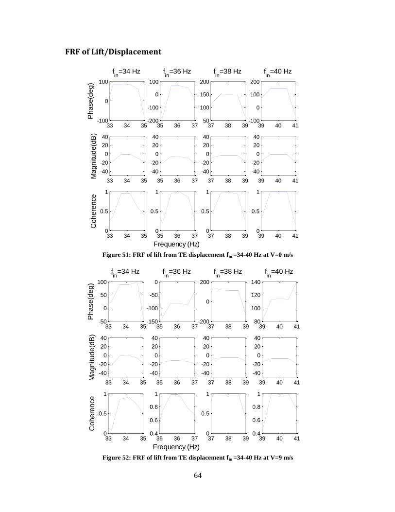
64

FRF of Lift/Displacement

Figure 51: FRF of lift from TE displacement fin =34-40 Hz at V=0 m/s

Figure 52: FRF of lift from TE displacement fin =34-40 Hz at V=9 m/s

33 34 350

0.5

1

Co

he

ren

ce

33 34 35

-40

-20

0

20

40

Ma

gn

itu

de

(dB

)

33 34 35-100

0

100

fin

=34 Hz

Ph

ase

(de

g)

35 36 370

0.5

1

Frequency (Hz)

35 36 37

-40

-20

0

20

40

35 36 37-200

-100

0

100

fin

=36 Hz

37 38 390

0.5

1

37 38 39

-40

-20

0

20

40

37 38 3950

100

150

200

fin

=38 Hz

39 40 410

0.5

1

39 40 41

-40

-20

0

20

40

39 40 41-100

0

100

200

fin

=40 Hz

33 34 350

0.5

1

Co

he

ren

ce

33 34 35

-40

-20

0

20

40

Ma

gn

itu

de

(dB

)

33 34 35-50

0

50

100

Ph

ase

(de

g)

fin

=34 Hz

35 36 370.4

0.6

0.8

1

Frequency (Hz)

35 36 37

-40

-20

0

20

40

35 36 37-150

-100

-50

0

fin

=36 Hz

37 38 390

0.5

1

37 38 39

-40

-20

0

20

40

37 38 39-200

0

200

fin

=38 Hz

39 40 410.4

0.6

0.8

1

39 40 41

-40

-20

0

20

40

39 40 4180

100

120

140

fin

=40 Hz

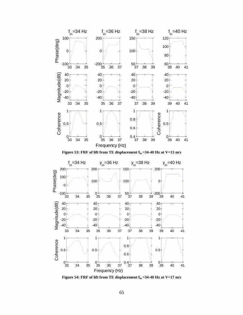
65

Figure 53: FRF of lift from TE displacement fin =34-40 Hz at V=13 m/s

Figure 54: FRF of lift from TE displacement fin =34-40 Hz at V=17 m/s

33 34 350

0.5

1

Co

he

ren

ce

33 34 35

-40

-20

0

20

40

Ma

gn

itu

de

(dB

)

33 34 35-100

0

100

Ph

ase

(de

g)

fin

=34 Hz

35 36 370

0.5

1

Frequency (Hz)

35 36 37

-40

-20

0

20

40

35 36 37-200

0

200

fin

=36 Hz

37 38 390.4

0.6

0.8

1

37 38 39

-40

-20

0

20

40

37 38 3950

100

150

fin

=38 Hz

39 40 410

0.5

1

Co

he

ren

ce

39 40 41

-40

-20

0

20

40

39 40 4160

80

100

120

fin

=40 Hz

33 34 350

0.5

1

Co

he

ren

ce

33 34 35

-40

-20

0

20

40

Ma

gn

itu

de

(dB

)

33 34 35-100

0

100

200

Ph

ase

(de

g)

fin

=34 Hz

35 36 370

0.5

1

Frequency (Hz)

35 36 37

-40

-20

0

20

40

35 36 370

100

200

yin

=36 Hz

37 38 390.4

0.6

0.8

1

37 38 39

-40

-20

0

20

40

37 38 3950

100

150

yin

=38 Hz

39 40 410

0.5

1

39 40 41

-40

-20

0

20

40

39 40 41-200

0

200

yin

=40 Hz