PHYSICS OF FLUIDS 29, 082109 (2017)

Characterization of interfacial waves and pressure dropin horizontal oil-water core-annular flows

Sumit Tripathi,1 Rico F. Tabor,2 Ramesh Singh,3 and Amitabh Bhattacharya3,a)1IITB-Monash Research Academy, Mumbai 400076, India2School of Chemistry, Monash University, Clayton 3800, Australia3Department of Mechanical Engineering, I.I.T. Bombay, Mumbai 400076, India

(Received 23 May 2017; accepted 29 July 2017; published online 18 August 2017)

We study the transportation of highly viscous furnace-oil in a horizontal pipe as core-annular flow(CAF) using experiments. Pressure drop and high-speed images of the fully developed CAF arerecorded for a wide range of flow rate combinations. The height profiles (with respect to the centerlineof the pipe) of the upper and lower interfaces of the core are obtained using a high-speed camera andimage analysis. Time series of the interface height are used to calculate the average holdup of the oilphase, speed of the interface, and the power spectra of the interface profile. We find that the ratio of theeffective velocity of the annular fluid to the core velocity, α, shows a large scatter. Using the averagevalue of this ratio (α = 0.74) yields a good estimate of the measured holdup for the whole range offlow rate ratios, mainly due to the low sensitivity of the holdup ratio to the velocity ratio. Dimensionalanalysis implies that, if the thickness of the annular fluid is much smaller than the pipe radius, then, forthe given range of parameters in our experiments, the non-dimensional interface shape, as well as thenon-dimensional wall shear stress, can depend only on the shear Reynolds number and the velocityratio. Our experimental data show that, for both lower and upper interfaces, the normalized powerspectrum of the interface height has a strong dependence on the shear Reynolds number. Specifically,for low shear Reynolds numbers, interfacial modes with large wavelengths dominate, while, for largeshear Reynolds numbers, interfacial modes with small wavelengths dominate. Normalized variance ofthe interface height is higher at lower shear Reynolds numbers and tends to a constant with increasingshear Reynolds number. Surprisingly, our experimental data also show that the effective wall shearstress is, to a large extent, proportional to the square of the core velocity. Using the implied scalingsfor the holdup ratio and wall shear stress, we can derive an expression for the pressure drop across thepipe in terms of the flow rates, which agrees well with our experimental measurements. Published byAIP Publishing. [http://dx.doi.org/10.1063/1.4998428]

I. INTRODUCTION

The high viscosity of heavy oil leads to large pressuredrops and energy requirements during its transport in pipelines.Conventional methods of reducing oil viscosity, e.g., mixingwith light oils or heating, are not cost-effective for the com-mercial pipeline transport of heavy-oil.1,2 It has long beensuggested that highly viscous fluids can be transported in awater-lubricated state, known as the core-annular flow (CAF),in which a lubricating layer of water is injected near the pipewall so that the oil does not come into direct contact with thewall. Lower wall shear stress, due to the much smaller viscos-ity of water flowing in the annular layer adjacent to the wall,drastically reduces (typically by 80%–95%) the effective pres-sure drop (and therefore, energy requirements) required forpumping the oil.

Experimental studies of oil–water CAF in pipes have beenextensively performed over the past few decades, by severalresearch groups.2–8 A major goal of these experiments has beento obtain an empirical relationship for the pressure drop acrossthe pipe, as well as the holdup ratio (or volume ratio), as afunction of water and oil flow rates. Arney et al.3 first observed

a)Author to whom correspondence should be addressed: bhattach@gmail.com

that the oil-to-water holdup ratio appears to depend only on theratio of oil and water flow rates and proposed a purely empiricalcorrelation based on their data. They also proposed correla-tions for the effective friction factor in a CAF in terms of aneffective Reynolds number by modifying relationships basedon a perfect core-annular flow (PCAF), where it is assumedthat the interface is undisturbed. A large scatter is observedin the experimental data on the effective friction factor, whencompared to the proposed correlations,3 which is attributed tothe higher eccentricity of the core at a lower Reynolds number.It is also not clear how theoretical relationships for a perfectcore-annular flow, where viscous stresses dominate the stressbalance, can be extended to wavy core-annular flows at highReynolds numbers, where pressure stresses at the oil–waterinterface may dominate over the viscous stresses. Rodriguezet al. have similarly proposed a modified pressure drop model,which accounts for slip ratio and buoyancy effects.9 Here, theyhave compared their model with data from literature and fieldexperiments, and they propose a correlation for the pressuredrop that uses expressions derived assuming PCAF.

The shape of the oil–water interface in CAF plays a keyrole in determining the overall pressure drop. Several theo-retical studies in the past have focused on understanding theevolution and steady-state solution of the interface profile.

1070-6631/2017/29(8)/082109/13/$30.00 29, 082109-1 Published by AIP Publishing.

082109-2 Tripathi et al. Phys. Fluids 29, 082109 (2017)

The linear stability analysis of CAFs10–13 have been extremelyvaluable for understanding the flow regimes where the inter-face becomes wavy. Miesen et al. have used analytical methodsto solve the growth rate problem of interfacial waves in CAF,and presented an asymptotic solution method.14 The shape ofthe interface predicted by stability analysis may agree wellwith experiments near the PCAF state. Direct numerical sim-ulation (DNS) of periodic wavy CAF,15 and numerical simu-lations of CAF in the lubrication limit16 have been performedpreviously. Both of these studies focused on connecting theshape of the interface with levitation of the core in horizontalCAF. They are however not able to provide a description ofthe interface at high flow rates, where the interface shape con-stantly evolves, and non-linear processes (e.g., merging andbreaking of waves) become important. Bannwart analyzed theinterfacial waves in CAF with kinetic wave theory, and com-pared the wave velocity (uw) with the core velocity (uc) inhorizontal and vertical CAFs.17 For a low density oil core, andwith the consideration of slip ratio, he reports that: uw > uc forthe vertical downward flow, uw < uc for the vertical upwardflow, and uw = uc for the horizontal flow.17 This work providesan interesting way to measure holdup in CAF using interfacialwave speed; however, it does not provide information on theshape of the interfacial waves.

In Ref. 18, the interface in an oil–water CAF was assumedto be periodic with a certain wavelength, and a constraintwas derived for the profile of the interface using the lubri-cation assumption. The constrained interface profile agreedwell with interface shapes recorded in experiments. Statisticson the interface profile were also reported in Ref. 18, althoughthese statistics were not linked to the pressure drop. Volume-of-fluid simulations of CAF in Ref. 19 confirmed some of theinterface characteristics reported in Ref. 18.

Several recent studies have reported interfacial waves instratified oil–water flows. Castro et al. characterized the inter-facial waves in a stratified oil–water flow in a pipe with respectto the two-phase Froude number.20 Al-Wahaibi and Angelihave used a conductivity probe and high speed imaging toobtain interfacial shape characteristics in such flows.21 Fur-ther, Barrel and Angeli have performed the spectral densityanalysis of stratified oil–water flows and have compared thecontributions of frequency ranges in the spectra at the inlet anddownstream test sections;22 here the focus was on understand-ing the dependence of the spectra on flow rate ratios. Whilemuch of the interfacial wave-dynamics of stratified oil–waterflows can be expected to be similar to that in CAF, the water-to-oil volume ratios in CAF are typically much smaller thanthe stratified oil–water flow. The dynamics of the interfacialwaves in CAF can therefore not be easily derived from thecharacterization of interfacial waves in stratified flows.

In the present work, we use experimental measurementsto characterize interfacial waves in the horizontal core-annularflow of oil and water. We use high viscosity furnace oil as thecore fluid and water as the annular fluid. We measure the pres-sure drop and record high resolution images of the interface fordifferent flow rate combinations, in a fully developed oil–waterCAF. The high speed images are analyzed, and the interfacialheight profiles of the upper and lower oil–water interfaces areextracted for each image. Temporal variation of the interface

height at a given location is then extracted from these images.Since the waves travel approximately with the speed of thecore, the spatial variation of the interface height, over a lengthmuch larger than the size of the viewing field, can also beextracted using the dynamic data. We calculate the holdup,average velocities (of core and annular fluids), and the powerspectrum of the interface height profile, for both the lower andupper interfaces. The pressure drop measurements are used tocalculate the effective wall shear stress for different oil–waterflow rates.

We reduce the experimental data by performing localizeddimensional analysis of the annular region, which is boundedby the interface and the pipe wall. We assume that the averagethickness of the annular region is negligible compared to theradius of the core fluid. The primary non-dimensional num-bers that emerge here are the shear Reynolds number Rec ofthe annulus (based on the kinematic viscosity of water, averageannular thickness, and speed of the core) and ratio α =Ua/Uc

of the average velocity of the annular fluid (Ua) to the aver-age velocity of the core fluid (Uc). We first relate the holdupratio in terms of flow rates and the average value of α overall the data sets, and, as observed earlier in Ref. 12, we findgood agreement between this model and the data. Next, we areable to show that the normalized power spectra of the inter-face height, as well as the normalized variance of interfaceheight, depend primarily on Rec. Finally, we observe that thewall shear stress, normalized by ρaU2

c (ρa is density of annu-lar fluid), depends weakly only on Rec. We use the scalingsthat emerge from our data to propose a closed-form empiri-cal relationship between the pressure drop and flow rates ofoil and water. Our approach is significantly different from pastefforts on characterizing the interface using experimental data,since we focus on using the localized interfacial dynamics inthe neighborhood of the annular region to explain the globalpressure drop. We do not use expressions for the pressure dropbased on the PCAF state and instead use the scalings predictedby empirical data to construct our model for the pressure drop.However, we note that several prior studies related to the linearstability analysis of the viscosity-stratified Couette flow23,24 douse a similar localized analysis of the annular layer to charac-terize the instability of the interface. Our results on the powerspectra of the interface height are consistent with the trendsfor most unstable modes predicted by these studies.

II. MATERIALS AND METHODSA. Experimental setup

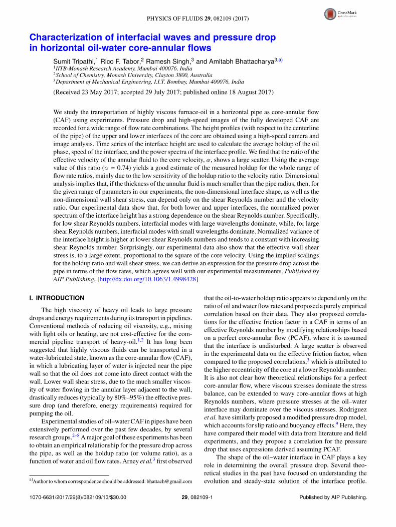
A schematic of the experiment setup is shown in Fig. 1.The flow-loop had three loft tanks (from Sintex): (i) a watertank of capacity 200 l, (ii) an oil tank of capacity 300 l, and(iii) a collector tank of capacity 500 l. Acrylic pipes of internaldiameter 15.5 mm and total length of about 5 m were usedfor the development and visualization of CAF. The length ofeach acrylic pipe was 2 m, and therefore flexible acrylic cou-plings were fabricated, to ensure smooth connection betweentwo pipes. All other connections were made with chlorinatedpolyvinyl chloride (CPVC) pipes of 3/4 in. internal diameter.All the pipe connections in the CPVC pipe loop were made

082109-3 Tripathi et al. Phys. Fluids 29, 082109 (2017)

FIG. 1. Schematic of the CAF experimental setup.

with standard 3/4 in. CPVC fittings (elbow, tee, couplings,unions, reducers, etc.). CPVC ball valves (size 3/4 in.) wereused at different places to redirect and/or control the flow ofboth the fluids. The flow rates of both the fluids (water and oil)were controlled by globe-valves (GVs) installed in respectiveloops, as shown in Fig. 1. The water was pumped with a cen-trifugal pump while the oil was pumped with a gear pump.A turbine type flow-meter was used to measure the flow rateof water, while an oval gear type flow meter was used forthe oil. Both the flow-meters were based on Hall effect sen-sors and gave output in terms of voltage pulses. Electronicpulse counter devices, one each for oil and water, were cali-brated to display the flow rates in liters per minute (lpm). Thepressure drop, across a length of 2 m in the fully developedsection, was measured with a differential pressure transmitter(DPT). The pressure drop and flow rate data were logged witha data acquisition system for different combinations of flowrates of oil and water. An acrylic visualization box was usedin the fully developed section (about 2.5 m from the injector),through which the acrylic pipe could pass, and then sealed toprevent any leakage of the fluid filled in it. This box was filledwith glycerol (a fluid whose refractive index is matched to thatof acrylic) to reduce the lens effect associated with the curva-ture of the acrylic pipe. A high speed CMOS camera (model:PCO 1200hs) was used to record images of the oil-water core-annular flow through the visualization box, at 1000 frames/s. A500 W halogen lamp was used to provide an adequate amountof light for image recording. Suitable supports were designedand fabricated to support the acrylic pipes, tanks, and CPVCpipes.

B. Design of water injector

The water was introduced into the acrylic pipe through aninjector which induces the CAF state by injecting the water

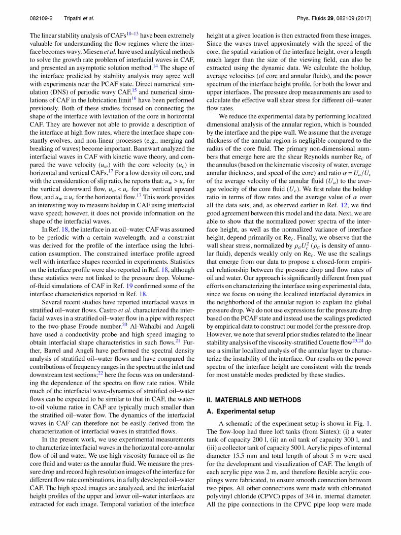
along the inside wall of the acrylic pipe. A schematic ofthe injector used in our experiment is shown in Fig. 2. Theinjector was made of two parts, which when assembled pro-vides a circumferential groove that acts as a reservoir forwater. Two inlets were made in the outer part of the injec-tor through which the water could fill the groove and flowuniformly along the inner wall of the pipe as the annular fluid.The injector components were fabricated from stainless steel(SS-316).

C. Pressure drop measurements

The pressure drop per unit length, ∂p∂z , was measured for

two different cases: (i) keeping Qa constant and varying Qc and(ii) keeping Qc constant and varying Qa. Here Qc is the volu-metric flow rate of the core fluid (oil) and Qa is the volumetricflow rate of the annular fluid (water). The experimental valuesof flow rates of oil and water for these two cases are shownin Tables I and II, respectively. The pressure drop measure-ments were performed with a differential pressure transmitter(DPT) across a length of two meters in the fully developedflow section of the acrylic pipe. The percentage reduction inthe pressure drop was estimated from the following equation

FIG. 2. Schematic of the annular fluid (water) injector.

082109-4 Tripathi et al. Phys. Fluids 29, 082109 (2017)

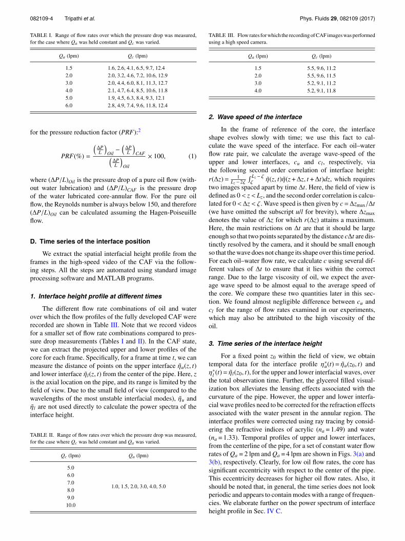
TABLE I. Range of flow rates over which the pressure drop was measured,for the case where Qa was held constant and Qc was varied.

Qa (lpm) Qc (lpm)

1.5 1.6, 2.6, 4.1, 6.5, 9.7, 12.42.0 2.0, 3.2, 4.6, 7.2, 10.6, 12.93.0 2.0, 4.4, 6.0, 8.1, 11.3, 12.74.0 2.1, 4.7, 6.4, 8.5, 10.6, 11.85.0 1.9, 4.5, 6.3, 8.4, 9.3, 12.16.0 2.8, 4.9, 7.4, 9.6, 11.8, 12.4

for the pressure reduction factor (PRF):2

PRF(%) =

(∆PL

)Oil−

(∆PL

)CAF(

∆PL

)Oil

× 100, (1)

where (∆P/L)Oil is the pressure drop of a pure oil flow (with-out water lubrication) and (∆P/L)CAF is the pressure dropof the water lubricated core-annular flow. For the pure oilflow, the Reynolds number is always below 150, and therefore(∆P/L)Oil can be calculated assuming the Hagen-Poiseuilleflow.

D. Time series of the interface position

We extract the spatial interfacial height profile from theframes in the high-speed video of the CAF via the follow-ing steps. All the steps are automated using standard imageprocessing software and MATLAB programs.

1. Interface height profile at different times

The different flow rate combinations of oil and waterover which the flow profiles of the fully developed CAF wererecorded are shown in Table III. Note that we record videosfor a smaller set of flow rate combinations compared to pres-sure drop measurements (Tables I and II). In the CAF state,we can extract the projected upper and lower profiles of thecore for each frame. Specifically, for a frame at time t, we canmeasure the distance of points on the upper interface ηu(z, t)and lower interface ηl(z, t) from the center of the pipe. Here, zis the axial location on the pipe, and its range is limited by thefield of view. Due to the small field of view (compared to thewavelengths of the most unstable interfacial modes), ηu andηl are not used directly to calculate the power spectra of theinterface height.

TABLE II. Range of flow rates over which the pressure drop was measured,for the case where Qc was held constant and Qa was varied.

Qc (lpm) Qa (lpm)

5.0

1.0, 1.5, 2.0, 3.0, 4.0, 5.0

6.07.08.09.010.0

TABLE III. Flow rates for which the recording of CAF images was performedusing a high speed camera.

Qa (lpm) Qc (lpm)

1.5 5.5, 9.6, 11.22.0 5.5, 9.6, 11.53.0 5.2, 9.1, 11.24.0 5.2, 9.1, 11.8

2. Wave speed of the interface

In the frame of reference of the core, the interfaceshape evolves slowly with time; we use this fact to cal-culate the wave speed of the interface. For each oil–waterflow rate pair, we calculate the average wave-speed of theupper and lower interfaces, cu and cl, respectively, viathe following second order correlation of interface height:r(∆z)= 1

Lz − 2ζ ∫Lz − ζζ η(z, t)η(z +∆z, t +∆t)dz, which requires

two images spaced apart by time ∆t. Here, the field of view isdefined as 0 < z < Lz, and the second order correlation is calcu-lated for 0 <∆z < ζ . Wave speed is then given by c=∆zmax/∆t(we have omitted the subscript u/l for brevity), where ∆zmax

denotes the value of ∆z for which r(∆z) attains a maximum.Here, the main restrictions on ∆t are that it should be largeenough so that two points separated by the distance c∆t are dis-tinctly resolved by the camera, and it should be small enoughso that the wave does not change its shape over this time period.For each oil–water flow rate, we calculate c using several dif-ferent values of ∆t to ensure that it lies within the correctrange. Due to the large viscosity of oil, we expect the aver-age wave speed to be almost equal to the average speed ofthe core. We compare these two quantities later in this sec-tion. We found almost negligible difference between cu andcl for the range of flow rates examined in our experiments,which may also be attributed to the high viscosity of theoil.

3. Time series of the interface height

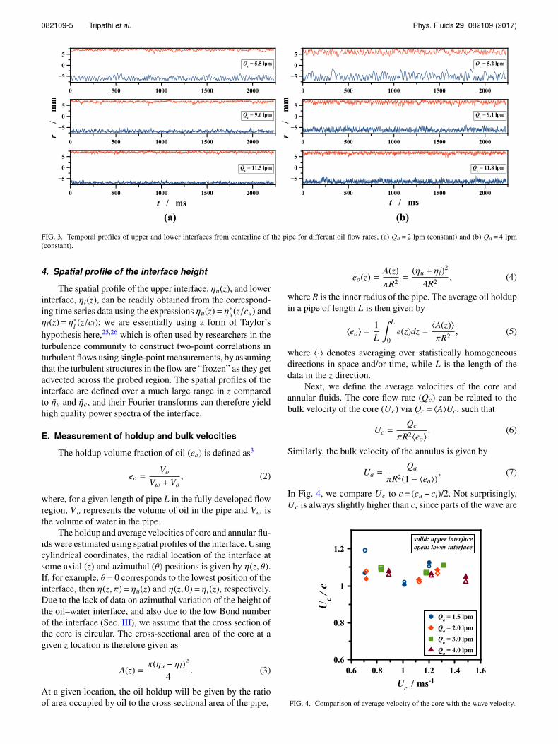
For a fixed point z0 within the field of view, we obtaintemporal data for the interface profile η∗u(t)= ηu(z0, t) andη∗l (t)= ηl(z0, t), for the upper and lower interfacial waves, overthe total observation time. Further, the glycerol filled visual-ization box alleviates the lensing effects associated with thecurvature of the pipe. However, the upper and lower interfa-cial wave profiles need to be corrected for the refraction effectsassociated with the water present in the annular region. Theinterface profiles were corrected using ray tracing by consid-ering the refractive indices of acrylic (na = 1.49) and water(na = 1.33). Temporal profiles of upper and lower interfaces,from the centerline of the pipe, for a set of constant water flowrates of Qa = 2 lpm and Qa = 4 lpm are shown in Figs. 3(a) and3(b), respectively. Clearly, for low oil flow rates, the core hassignificant eccentricity with respect to the center of the pipe.This eccentricity decreases for higher oil flow rates. Also, itshould be noted that, in general, the time series does not lookperiodic and appears to contain modes with a range of frequen-cies. We elaborate further on the power spectrum of interfaceheight profile in Sec. IV C.

082109-5 Tripathi et al. Phys. Fluids 29, 082109 (2017)

FIG. 3. Temporal profiles of upper and lower interfaces from centerline of the pipe for different oil flow rates, (a) Qa = 2 lpm (constant) and (b) Qa = 4 lpm(constant).

4. Spatial profile of the interface height

The spatial profile of the upper interface, ηu(z), and lowerinterface, ηl(z), can be readily obtained from the correspond-ing time series data using the expressions ηu(z)= η∗u(z/cu) andηl(z)= η∗l (z/cl); we are essentially using a form of Taylor’shypothesis here,25,26 which is often used by researchers in theturbulence community to construct two-point correlations inturbulent flows using single-point measurements, by assumingthat the turbulent structures in the flow are “frozen” as they getadvected across the probed region. The spatial profiles of theinterface are defined over a much large range in z comparedto ηu and ηc, and their Fourier transforms can therefore yieldhigh quality power spectra of the interface.

E. Measurement of holdup and bulk velocities

The holdup volume fraction of oil (eo) is defined as3

eo =Vo

Vw + Vo, (2)

where, for a given length of pipe L in the fully developed flowregion, Vo represents the volume of oil in the pipe and Vw isthe volume of water in the pipe.

The holdup and average velocities of core and annular flu-ids were estimated using spatial profiles of the interface. Usingcylindrical coordinates, the radial location of the interface atsome axial (z) and azimuthal (θ) positions is given by η(z, θ).If, for example, θ = 0 corresponds to the lowest position of theinterface, then η(z, π)= ηu(z) and η(z, 0)= ηl(z), respectively.Due to the lack of data on azimuthal variation of the height ofthe oil–water interface, and also due to the low Bond numberof the interface (Sec. III), we assume that the cross section ofthe core is circular. The cross-sectional area of the core at agiven z location is therefore given as

A(z) =π(ηu + ηl)2

4. (3)

At a given location, the oil holdup will be given by the ratioof area occupied by oil to the cross sectional area of the pipe,

eo(z) =A(z)

πR2=

(ηu + ηl)2

4R2, (4)

where R is the inner radius of the pipe. The average oil holdupin a pipe of length L is then given by

〈eo〉 =1L

∫ L

0e(z)dz =

〈A(z)〉

πR2, (5)

where 〈·〉 denotes averaging over statistically homogeneousdirections in space and/or time, while L is the length of thedata in the z direction.

Next, we define the average velocities of the core andannular fluids. The core flow rate (Qc) can be related to thebulk velocity of the core (Uc) via Qc = 〈A〉Uc, such that

Uc =Qc

πR2〈eo〉. (6)

Similarly, the bulk velocity of the annulus is given by

Ua =Qa

πR2(1 − 〈eo〉). (7)

In Fig. 4, we compare Uc to c = (cu + cl)/2. Not surprisingly,Uc is always slightly higher than c, since parts of the wave are

FIG. 4. Comparison of average velocity of the core with the wave velocity.

082109-6 Tripathi et al. Phys. Fluids 29, 082109 (2017)

located closer to the pipe wall, where the speed should neces-sarily be smaller. On average, the two values differ by 7%, andthe maximum deviation is around 20% for small values of Qa

and high values of Qc/Qa. These data confirm that the interfa-cial waves are almost stationary with respect to the frame ofreference of the core, most likely due to the high viscosity ofthe oil.

III. DIMENSIONAL ANALYSIS OF ANNULAR REGION

We primarily characterize the interface using the dimen-sional analysis of the annular region of the CAF. We are inter-ested in obtaining empirical relationships for the fluctuation inthe interface profile,

η ′(z) = η(z) − 〈η〉 (8)

(along with its associated statistics), as well as the effectivewall shear stress τ, which, for fully developed CAF, is relatedto the pressure drop by

τ =R2∂p∂z

, (9)

in terms of the other independent parameters that control theinterfacial flow in the annulus. We favor modeling τ over ∂p

∂x ,since it is a localized quantity within the annulus. However,we must also note that the above definition for τ representsthe circumferential average of wall shear stress and that in

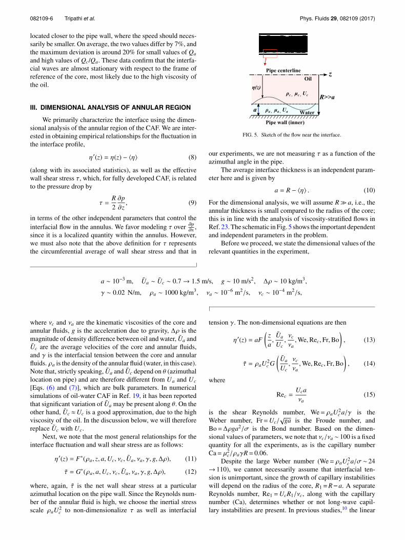
FIG. 5. Sketch of the flow near the interface.

our experiments, we are not measuring τ as a function of theazimuthal angle in the pipe.

The average interface thickness is an independent param-eter here and is given by

a = R − 〈η〉 . (10)

For the dimensional analysis, we will assume R� a, i.e., theannular thickness is small compared to the radius of the core;this is in line with the analysis of viscosity-stratified flows inRef. 23. The schematic in Fig. 5 shows the important dependentand independent parameters in the problem.

Before we proceed, we state the dimensional values of therelevant quantities in the experiment,

a ∼ 10−3 m, Ua ∼ Uc ∼ 0.7→ 1.5 m/s, g ∼ 10 m/s2, ∆ρ ∼ 10 kg/m3,

γ ∼ 0.02 N/m, ρa ∼ 1000 kg/m3, νa ∼ 10−6 m2/s, νc ∼ 10−4 m2/s,

where νc and νa are the kinematic viscosities of the core andannular fluids, g is the acceleration due to gravity, ∆ρ is themagnitude of density difference between oil and water, Ua andUc are the average velocities of the core and annular fluids,and γ is the interfacial tension between the core and annularfluids. ρa is the density of the annular fluid (water, in this case).Note that, strictly speaking, Ua and Uc depend on θ (azimuthallocation on pipe) and are therefore different from Ua and Uc

[Eqs. (6) and (7)], which are bulk parameters. In numericalsimulations of oil-water CAF in Ref. 19, it has been reportedthat significant variation of Ua may be present along θ. On theother hand, Uc ≈Uc is a good approximation, due to the highviscosity of the oil. In the discussion below, we will thereforereplace Uc with Uc.

Next, we note that the most general relationships for theinterface fluctuation and wall shear stress are as follows:

η ′(z) = F∗(ρa, z, a, Uc, νc, Ua, νa, γ, g,∆ρ), (11)

τ = G∗(ρa, a, Uc, νc, Ua, νa, γ, g,∆ρ), (12)

where, again, τ is the net wall shear stress at a particularazimuthal location on the pipe wall. Since the Reynolds num-ber of the annular fluid is high, we choose the inertial stressscale ρaU2

c to non-dimensionalize τ as well as interfacial

tension γ. The non-dimensional equations are then

η ′(z) = aF

(za

,Ua

Uc,νc

νa, We, Rec, Fr, Bo

), (13)

τ = ρaU2c G

(Ua

Uc,νc

νa, We, Rec, Fr, Bo

), (14)

where

Rec =Ucaνa

(15)

is the shear Reynolds number, We= ρaU2c a/γ is the

Weber number, Fr=Uc/√

ga is the Froude number, andBo=∆ρga2/σ is the Bond number. Based on the dimen-sional values of parameters, we note that νc/νa ∼ 100 is a fixedquantity for all the experiments, as is the capillary numberCa= µ2

c/ρaγR= 0.06.Despite the large Weber number (We= ρaU2

c a/σ ∼ 24→ 110), we cannot necessarily assume that interfacial ten-sion is unimportant, since the growth of capillary instabilitieswill depend on the radius of the core, R1 = R � a. A separateReynolds number, Re1 =UcR1/νc, along with the capillarynumber (Ca), determines whether or not long-wave capil-lary instabilities are present. In previous studies,10 the linear

082109-7 Tripathi et al. Phys. Fluids 29, 082109 (2017)

stability analysis of CAF was used to show that surface ten-sion can lead to unstable long-wave modes for Re1 <Recr

1 ,where Recr

1 = β(Ca)−1/2, and β is a constant that depends onthe parameters a/R1, νa/νc. High shear rates stabilize the flowfor Re1 >Recr

1 . For the parameter range relevant to our experi-ments (νa/νc→ 0, 0.05< a/R1 < 0.3), it has been shown10 thatβ ∈ [0.8, 1.4], and therefore Recr

1 < 15. For our experiments,Re1 ∈ [30, 60], and therefore we do not expect to see interfacialinstability due to interfacial tension.

The Froude number is large (Fr∼ 7→ 15), implying thatgravity does not directly affect interfacial dynamics in theannular region. The Bond number is small (Bo∼ 5× 10−3),implying that surface tension dominates gravitational forceswithin the annular region. In horizontal CAF, the Froude num-ber and Bond number based on the core radius R1 (insteadof a) together determine the eccentricity of the core and theaverage cross-sectional shape of the core, respectively. TheBond number based on R1 is around 0.2, implying that theaverage cross section of the core should be approximately acircle.

In our experiments, where νa/νc and Ca are constant, wecan simplify Eqs. (11) and (12) to

η ′(z) = aF

(za

,Ua

Uc, Rec

), (16)

τ = ρaU2c G

(Ua

Uc, Rec

). (17)

In the rest of the paper, we will further characterize η ′(z) andτ using the above non-dimensional forms. In our experiments,we do not explicitly measure Ua/Uc; however, as we will seebelow, the relevant non-dimensional flow and interfacial statis-tics appear to depend more strongly on Rec, for which wehave been able to take accurate measurements. Similarly, eventhough we do not measure τ in our experiments, we will findthat the net wall shear stress depends strongly only on Uc,which does not vary azimuthally.

IV. RESULTS AND DISCUSSIONA. Flow development and pressure drop

Representative images showing the development of thecore-annular flow for a fixed value of Qa are shown in Fig. 6.At low oil flow rates, we observe the formation of small slugsin the core [Fig. 6(a)]. As the oil flow rate is increased, theseslugs combine to experience lower drag and coalesce with eachother, forming longer slugs [Fig. 6(b)]. A further increase inthe oil flow rate typically results in the core-annular flow witha continuous core [Figs. 6(c)–6(f)]. The eccentricity of thecore with respect to the center of the pipe reduces at higherflow rate ratios of oil to water, although we do not present asystematic study of eccentricity in this paper. The images inFig. 6 were obtained using a high speed camera operating at1000 frames/s.

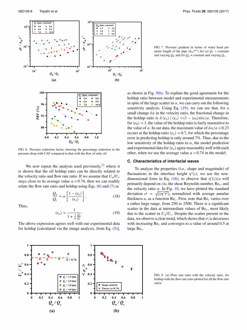
The pressure drop, in terms of water head per meter lengthof pipe (hwl�1), for different flow rate combinations, is shownin Figs. 7(a) and 7(b). Figure 7(a) represents six different cases

FIG. 6. Development of the core-annular flow for Qa = 3 lpm (constant) andQc (lpm) as (a) 0.8, (b) 1.3, (c) 3.5, (d) 5.2, (e) 9.1, and (f) 11.2.

where Qc is kept constant and Qa is varied while Fig. 7(b)shows six complementary cases where Qa is held constant andQc is varied. The plots here compare well with similar datapresented in Figs. 5–7 in the work of Arney et al.,3 wherecrude oil and fuel oil were used as core fluids, and the pipehad inner diameter very similar to our setup. The percent-age reduction in the pressure drop in terms of the pressurereduction factor (PRF), calculated using Eq. (1), is shown inFig. 8. It can be seen that the pressure drop with water-lubrication can be typically reduced by up to 97%, when com-pared to the pressure drop required to pump only oil. Therefore,as reported by numerous researchers in the past,2–6 the pres-sure drop (and therefore power) required to transport highlyviscous oil can indeed be significantly reduced by injectingwater in the annulus.

B. Velocity and holdup ratios

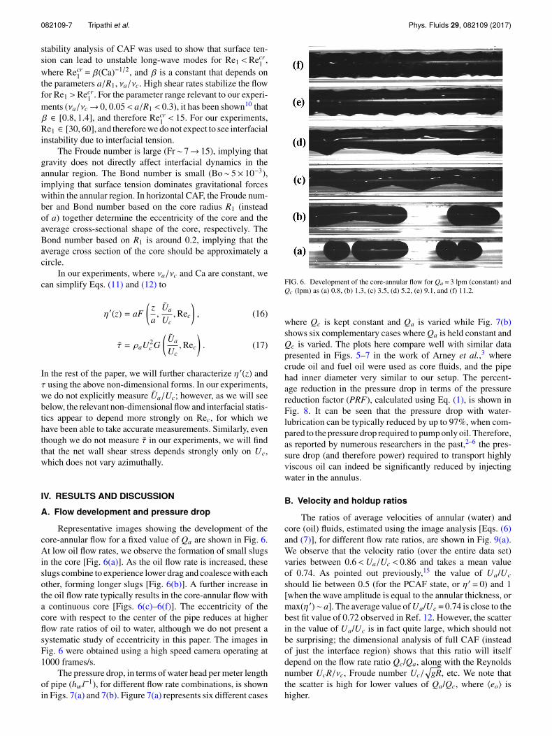
The ratios of average velocities of annular (water) andcore (oil) fluids, estimated using the image analysis [Eqs. (6)and (7)], for different flow rate ratios, are shown in Fig. 9(a).We observe that the velocity ratio (over the entire data set)varies between 0.6<Ua/Uc < 0.86 and takes a mean valueof 0.74. As pointed out previously,15 the value of Ua/Uc

should lie between 0.5 (for the PCAF state, or η ′ = 0) and 1[when the wave amplitude is equal to the annular thickness, ormax(η ′)∼ a]. The average value of Ua/Uc = 0.74 is close to thebest fit value of 0.72 observed in Ref. 12. However, the scatterin the value of Ua/Uc is in fact quite large, which should notbe surprising; the dimensional analysis of full CAF (insteadof just the interface region) shows that this ratio will itselfdepend on the flow rate ratio Qc/Qa, along with the Reynoldsnumber UcR/νc, Froude number Uc/

√gR, etc. We note that

the scatter is high for lower values of Qa/Qc, where 〈eo〉 ishigher.

082109-8 Tripathi et al. Phys. Fluids 29, 082109 (2017)

FIG. 7. Pressure gradient in terms of water head permeter length of the pipe (hw l�1) for (a) Qc = constantand varying Qa and (b) Qa = constant and varying Qc.

FIG. 8. Pressure reduction factor, showing the percentage reduction in thepressure drop with CAF compared to that with the flow of only oil.

We now repeat the analysis used previously,12 where itis shown that the oil holdup ratio can be directly related tothe velocity ratio and flow rate ratio. If we assume that Ua/Uc

stays close to its average value α = 0.74, then we can readilyrelate the flow rate ratio and holdup using Eqs. (6) and (7) as

Qa

Qc= α

[1 − 〈eo〉

〈eo〉

]. (18)

Thus,

〈eo〉 =1

1 + 1α

QaQc

. (19)

The above expression agrees well with our experimental datafor holdup [calculated via the image analysis, from Eq. (5)],

as shown in Fig. 9(b). To explain the good agreement for theholdup ratio between model and experimental measurementsin spite of the large scatter in α, we can carry out the followingsensitivity analysis. Using Eq. (19), we can see that, for asmall change δα in the velocity ratio, the fractional change inthe holdup ratio is δ 〈eo〉 / 〈eo〉 ≈ (1 − 〈e0〉)δα/α. Therefore,for 〈e0〉 ≈ 1, the value of the holdup ratio is fairly insensitive tothe value of α. In our data, the maximum value of δα/α ≈ 0.23occurs at the holdup ratio 〈eo〉 ≈ 0.7, for which the percentageerror in predicting holdup is only around 7%. Thus, due to thelow sensitivity of the holdup ratio to α, the model predictionand experimental data for 〈eo〉 agree reasonably well with eachother, when we use the average value α = 0.74 in the model.

C. Characteristics of interfacial waves

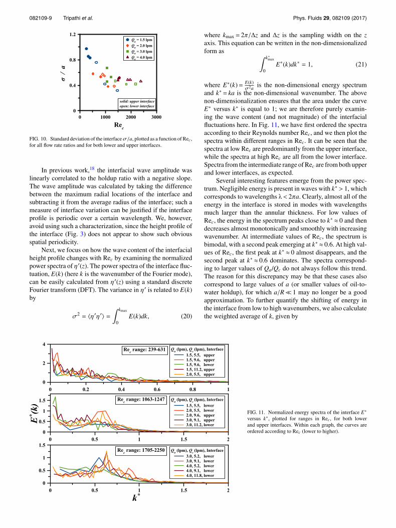
To analyze the properties (i.e., shape and magnitude) offluctuations in the interface height η ′(z), we use the non-dimensional form in Eq. (16), to observe that η ′(z)/a willprimarily depend on z/a, the shear Reynolds number, Rec, andthe velocity ratio α. In Fig. 10, we have plotted the standarddeviation σ =

√⟨(η ′)2⟩, normalized with average annular

thickness a, as a function Rec. First, note that Rec varies overa rather large range, from 250 to 2500. There is a significantscatter in the data at intermediate values of Rec, most likelydue to the scatter in Ua/Uc. Despite the scatter present in thedata, we observe a clear trend, which shows thatσ/a decreaseswith increasing Rec and converges to a value of around 0.5 atlarge Rec.

FIG. 9. (a) Flow rate ratio with the velocity ratio, (b)holdup with the flow rate ratio plotted for all the flow rateratios.

082109-9 Tripathi et al. Phys. Fluids 29, 082109 (2017)

FIG. 10. Standard deviation of the interfaceσ/a, plotted as a function of Rec,for all flow rate ratios and for both lower and upper interfaces.

In previous work,18 the interfacial wave amplitude waslinearly correlated to the holdup ratio with a negative slope.The wave amplitude was calculated by taking the differencebetween the maximum radial locations of the interface andsubtracting it from the average radius of the interface; such ameasure of interface variation can be justified if the interfaceprofile is periodic over a certain wavelength. We, however,avoid using such a characterization, since the height profile ofthe interface (Fig. 3) does not appear to show such obviousspatial periodicity.

Next, we focus on how the wave content of the interfacialheight profile changes with Rec by examining the normalizedpower spectra of η ′(z). The power spectra of the interface fluc-tuation, E(k) (here k is the wavenumber of the Fourier mode),can be easily calculated from η ′(z) using a standard discreteFourier transform (DFT). The variance in η ′ is related to E(k)by

σ2 = 〈η ′η ′〉 =

∫ kmax

0E(k)dk, (20)

where kmax = 2π/∆z and ∆z is the sampling width on the zaxis. This equation can be written in the non-dimensionalizedform as ∫ k∗max

0E∗(k)dk∗ = 1, (21)

where E∗(k)= E(k)σ2a

is the non-dimensional energy spectrumand k∗ = ka is the non-dimensional wavenumber. The abovenon-dimensionalization ensures that the area under the curveE∗ versus k∗ is equal to 1; we are therefore purely examin-ing the wave content (and not magnitude) of the interfacialfluctuations here. In Fig. 11, we have first ordered the spectraaccording to their Reynolds number Rec, and we then plot thespectra within different ranges in Rec. It can be seen that thespectra at low Rec are predominantly from the upper interface,while the spectra at high Rec are all from the lower interface.Spectra from the intermediate range of Rec are from both upperand lower interfaces, as expected.

Several interesting features emerge from the power spec-trum. Negligible energy is present in waves with k∗ > 1, whichcorresponds to wavelengths λ< 2πa. Clearly, almost all of theenergy in the interface is stored in modes with wavelengthsmuch larger than the annular thickness. For low values ofRec, the energy in the spectrum peaks close to k∗ ≈ 0 and thendecreases almost monotonically and smoothly with increasingwavenumber. At intermediate values of Rec, the spectrum isbimodal, with a second peak emerging at k∗ ≈ 0.6. At high val-ues of Rec, the first peak at k∗ ≈ 0 almost disappears, and thesecond peak at k∗ ≈ 0.6 dominates. The spectra correspond-ing to larger values of Qa/Qc do not always follow this trend.The reason for this discrepancy may be that these cases alsocorrespond to large values of a (or smaller values of oil-to-water holdup), for which a/R� 1 may no longer be a goodapproximation. To further quantify the shifting of energy inthe interface from low to high wavenumbers, we also calculatethe weighted average of k, given by

FIG. 11. Normalized energy spectra of the interface E∗

versus k∗, plotted for ranges in Rec, for both lowerand upper interfaces. Within each graph, the curves areordered according to Rec (lower to higher).

082109-10 Tripathi et al. Phys. Fluids 29, 082109 (2017)

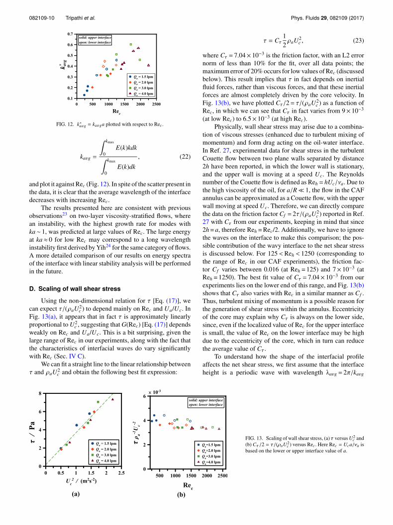
FIG. 12. k∗avg = kavga plotted with respect to Rec.

kavg =

∫ kmax

0E(k)kdk∫ kmax

0E(k)dk

, (22)

and plot it against Rec (Fig. 12). In spite of the scatter present inthe data, it is clear that the average wavelength of the interfacedecreases with increasing Rec.

The results presented here are consistent with previousobservations23 on two-layer viscosity-stratified flows, wherean instability, with the highest growth rate for modes withka∼ 1, was predicted at large values of Rec. The large energyat ka≈ 0 for low Rec may correspond to a long wavelengthinstability first derived by Yih24 for the same category of flows.A more detailed comparison of our results on energy spectraof the interface with linear stability analysis will be performedin the future.

D. Scaling of wall shear stress

Using the non-dimensional relation for τ [Eq. (17)], wecan expect τ/(ρaU2

c ) to depend mainly on Rec and Ua/Uc. InFig. 13(a), it appears that in fact τ is approximately linearlyproportional to U2

c , suggesting that G(Rec) [Eq. (17)] dependsweakly on Rec and Ua/Uc. This is a bit surprising, given thelarge range of Rec in our experiments, along with the fact thatthe characteristics of interfacial waves do vary significantlywith Rec (Sec. IV C).

We can fit a straight line to the linear relationship betweenτ and ρaU2

c and obtain the following best fit expression:

τ = Cτ12ρaU2

c , (23)

where Cτ = 7.04× 10−3 is the friction factor, with an L2 errornorm of less than 10% for the fit, over all data points; themaximum error of 20% occurs for low values of Rec (discussedbelow). This result implies that τ in fact depends on inertialfluid forces, rather than viscous forces, and that these inertialforces are almost completely driven by the core velocity. InFig. 13(b), we have plotted Cτ/2= τ/(ρaU2

c ) as a function ofRec, in which we can see that Cτ in fact varies from 9× 10−3

(at low Rec) to 6.5× 10−3 (at high Rec).Physically, wall shear stress may arise due to a combina-

tion of viscous stresses (enhanced due to turbulent mixing ofmomentum) and form drag acting on the oil-water interface.In Ref. 27, experimental data for shear stress in the turbulentCouette flow between two plane walls separated by distance2h have been reported, in which the lower wall is stationary,and the upper wall is moving at a speed Uc. The Reynoldsnumber of the Couette flow is defined as Reh = hUc/νa. Due tothe high viscosity of the oil, for a/R� 1, the flow in the CAFannulus can be approximated as a Couette flow, with the upperwall moving at speed Uc. Therefore, we can directly comparethe data on the friction factor Cf = 2τ/(ρaU2

c ) reported in Ref.27 with Cτ from our experiments, keeping in mind that since2h = a, therefore Reh = Rec/2. Additionally, we have to ignorethe waves on the interface to make this comparison; the pos-sible contribution of the wavy interface to the net shear stressis discussed below. For 125<Reh < 1250 (corresponding tothe range of Rec in our CAF experiments), the friction fac-tor Cf varies between 0.016 (at Reh = 125) and 7× 10−3 (atReh = 1250). The best fit value of Cτ = 7.04× 10−3 from ourexperiments lies on the lower end of this range, and Fig. 13(b)shows that Cτ also varies with Rec in a similar manner as Cf .Thus, turbulent mixing of momentum is a possible reason forthe generation of shear stress within the annulus. Eccentricityof the core may explain why Cτ is always on the lower side,since, even if the localized value of Rec for the upper interfaceis small, the value of Rec on the lower interface may be highdue to the eccentricity of the core, which in turn can reducethe average value of Cτ .

To understand how the shape of the interfacial profileaffects the net shear stress, we first assume that the interfaceheight is a periodic wave with wavelength λavg = 2π/kavg

FIG. 13. Scaling of wall shear stress, (a) τ versus U2c and

(b) Cτ/2 = τ/(ρaU2c ) versus Rec. Here Rec = Uca/νa is

based on the lower or upper interface value of a.

082109-11 Tripathi et al. Phys. Fluids 29, 082109 (2017)

and with amplitude proportional to σ. In the context of ourexperiments, kavg and σ have already been defined and char-acterized earlier in Sec. IV C. We again assume that the coreis moving like a solid body, with velocity Uc, and that theflow in the annulus is completely driven by the core veloc-ity; in effect, we are assuming that the flow in the annulus issimilar to the Couette flow between a wavy upper wall that ismoving and a flat lower wall which is stationary. This is a fairassumption, since the effect of the mean axial pressure gradi-ent will be small in the thin annulus, compared to the effect ofthe local pressure distribution induced by the interface shape.Dimensional analysis shows that the percentage of stress dueto form drag is then a function of σkavg, as well as kavga. Inour experiments (Sec. IV C), we observe that σkavg ∈ [0.1 0.3]and 0 < kavga < 1. There is little direct experimental or com-putational data on how the percentage of stress due to formdrag depends on these parameters, even in the prior literatureon DNS of CAFs.15,28 In Ref. 29, DNS of the Couette flowover wavy walls at a high Reynolds number was carried out,where it was observed that the percentage of shear stress due toform drag increases with increasing kavgσ and reaches around20% of the net shear stress for kavgσ ∼ 0.2. However, for thesesimulations, kavga= 2π was used, which, for a fixed value ofkavgσ, corresponds to a much smaller blockage ratio of theannular gap compared to our experiments, where kavga < 1.We expect the percentage of shear stress due to form drag tobe higher in our experiments because of the larger blockageratios, but we are not able to give a clear quantitative estimateof this percentage due to the lack of prior data. At any rate, itappears that the friction factor Cτ depends weakly on Rec, eventhough the percentage of form drag and viscous drag actingon the interface may vary with flow parameters.

E. Pressure drop vs. flow rate relationship

In this section, we use the inertial scaling for τ [Eq.(23)], along with the model for holdup [Eq. (19)] to obtain an

expression for pressure drop ∂p∂z in terms of flow rates Qa and

Qc. Equation (23) along with the definition for Uc [Eq. (6)]and holdup 〈eo〉 [Eq. (5)] yields

τ = Cτ12ρa

Q2c

〈A〉2= Cτ

12ρa

Q2c

π2R4〈eo〉2

. (24)

We next use the relationship between τ and p [Eq. (9)], alongwith the model for holdup [Eq. (19)] to obtain a model forpressure gradient,

∂p∂z=

Cτ ρa

π2

Q2c

R5

[1 +

1α

Qa

Qc

]2

. (25)

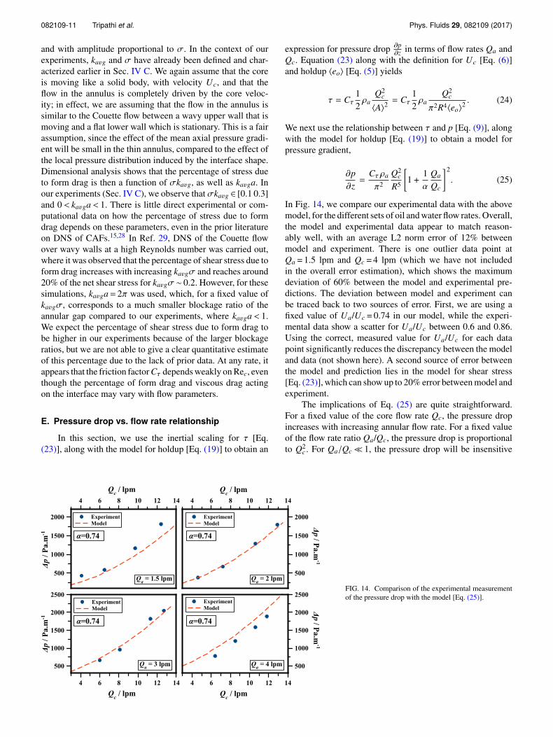
In Fig. 14, we compare our experimental data with the abovemodel, for the different sets of oil and water flow rates. Overall,the model and experimental data appear to match reason-ably well, with an average L2 norm error of 12% betweenmodel and experiment. There is one outlier data point atQa = 1.5 lpm and Qc = 4 lpm (which we have not includedin the overall error estimation), which shows the maximumdeviation of 60% between the model and experimental pre-dictions. The deviation between model and experiment canbe traced back to two sources of error. First, we are using afixed value of Ua/Uc = 0.74 in our model, while the experi-mental data show a scatter for Ua/Uc between 0.6 and 0.86.Using the correct, measured value for Ua/Uc for each datapoint significantly reduces the discrepancy between the modeland data (not shown here). A second source of error betweenthe model and prediction lies in the model for shear stress[Eq. (23)], which can show up to 20% error between model andexperiment.

The implications of Eq. (25) are quite straightforward.For a fixed value of the core flow rate Qc, the pressure dropincreases with increasing annular flow rate. For a fixed valueof the flow rate ratio Qa/Qc, the pressure drop is proportionalto Q2

c . For Qa/Qc� 1, the pressure drop will be insensitive

FIG. 14. Comparison of the experimental measurementof the pressure drop with the model [Eq. (25)].

082109-12 Tripathi et al. Phys. Fluids 29, 082109 (2017)

to the flow rate ratio and will again be proportional to Q2c . The

pressure drop does not explicitly depend on the viscosity ofthe annular fluid, as long as Rec is large enough. Equation (25)will probably not hold at very low values of Qa/Qc, where thecore starts to foul the pipe wall.

The viscosity ratio νc/νa should affect the dominantmodes in the interface height profile. However, based on ourexperimental data, it appears that the friction factor Cτ dependsweakly on the wave content of the interface height profile.Therefore, we expect the pressure drop itself to depend weaklyon the viscosity ratio of the core and annular fluid, over a widerange of viscosity ratios. However, we will need to performadditional experiments with different core fluids to completelycharacterize this dependence.

V. CONCLUSION

In this work, we have presented a novel localized anal-ysis of experimental data of the annular region in the core-annular flow (CAF). It is clear that the oil-water interfaceshape is strongly dependent on the shear Reynolds numberRec. Specifically, the wavelength of the most dominant modeof the interface, normalized by the annular thickness, reduceswith increasing Rec and tends to a constant value at largeRec. Another major insight from our data is that the effec-tive wall shear stress τ appears to depend linearly on ρaU2

c .More specifically, the friction factor, Cτ = 2τ/(ρaU2

c ), dependsweakly on the shear Reynolds number Rec. Due to the lackof measurements and prior data on the how the pressureand viscous stresses are related to the shape of the inter-face, it is not possible to exactly link the interface shape tothe net wall shear stress. However, it is plausible that vis-cous stresses, enhanced by turbulent mixing of momentumin the annulus, as well as form drag acting on the interface,are responsible for the net shear stress. We also found thata reasonably good agreement between experimental data andmodel for the oil holdup fraction can be obtained by usingan averaged value for the ratio of annular to core velocity,α. Using the model for oil holdup and the scaling τ ∼ ρaU2

cemerging from our experiments, we are able to build a semi-empirical model for the pressure drop that matches well withthe experimental measurements for a large range of parame-ters. Given that the interface height profile is in fact composedof modes spanning a range of wavelengths, a more thoroughunderstanding of the relationship between drag acting on theinterfacial waves and the power spectra of the interfacial wavesis required here. The scatter in values of annular-to-core veloc-ity, α, is a major source of discrepancy between model andexperimental measurements of both the holdup-ratio and wallshear stress. In the future, we will attempt to understand howthis ratio depends on the various independent parameters inCAF.

ACKNOWLEDGMENTS

The authors are grateful to Orica Limited (Australia) forfinancial support and useful discussion on the injector design.The authors are also thankful to the PIV Lab, Mechanical

Engineering Department, IIT Bombay for providing space forthe experimental setup.

1G. Ooms, A. Segal, A. Van Der Wees, R. Meerhoff, and R. Oliemans, “Atheoretical model for core-annular flow of a very viscous oil core and awater annulus through a horizontal pipe,” Int. J. Multiphase Flow 10, 41–60(1983).

2A. Bensakhria, Y. Peysson, and G. Antonini, “Experimental study of thepipeline lubrication for heavy oil transport,” Oil Gas Sci. Technol. 59, 523–533 (2004).

3M. Arney, R. Bai, E. Guevara, D. Joseph, and K. Liu, “Friction factor andholdup studies for lubricated pipelining. Experiments and correlations,” Int.J. Multiphase Flow 19, 1061–1076 (1993).

4A. Huang, C. Christodoulou, and D. D. Joseph, “Friction fractor and holdupstudies for lubricated pipelining—II laminar and kεmodels of eccentric coreflow,” Int. J. Multiphase Flow 20, 481–491 (1994).

5G. Sotgia, P. Tartarini, and E. Stalio, “Experimental analysis of flow regimesand pressure drop reduction in oil–water mixtures,” Int. J. Multiphase Flow34, 1161–1174 (2008).

6D. Strazza, B. Grassi, M. Demori, V. Ferrari, and P. Poesio, “Core-annularflow in horizontal and slightly inclined pipes: Existence, pressure drops,and hold-up,” Chem. Eng. Sci. 66, 2853–2863 (2011).

7D. D. Joseph, R. Bai, K. Chen, and Y. Y. Renardy, “Core-annular flows,”Annu. Rev. Fluid Mech. 29, 65–90 (1997).

8S. Ghosh, T. Mandal, G. Das, and P. Das, “Review of oil watercore annular flow,” Renewable Sustainable Energy Rev. 13, 1957–1965(2009).

9O. Rodriguez, A. Bannwart, and C. De Carvalho, “Pressure loss incore-annular flow: Modeling, experimental investigation and full-scaleexperiments,” J. Pet. Sci. Eng. 65, 67–75 (2009).

10L. Preziosi, K. Chen, and D. D. Joseph, “Lubricated pipelining: Stability ofcore-annular flow,” J. Fluid Mech. 201, 323–356 (1989).

11H. H. Hu and D. D. Joseph, “Lubricated pipelining: Stability of core-annularflow. Part 2,” J. Fluid Mech. 205, 359–396 (1989).

12R. Bai, K. Chen, and D. D. Joseph, “Lubricated pipelining: Stability ofcore-annular flow. Part 5. Experiments and comparison with theory,” J.Fluid Mech. 240, 97–132 (1992).

13D. Joseph and Y. Renardy, Fundamentals of Two-Fluids Dynamics. PartII: Lubricated Transport, Drops and Miscible Liquids (Springer ScienceBusiness Media, LLC, 1993).

14R. Miesen, G. Beijnon, P. E. M. Duijvestijn, R. V. A. Oliemans, andT. Verheggen, “Interfacial waves in core-annular flow,” J. Fluid Mech. 238,97–117 (1992).

15R. Bai, K. Kelkar, and D. D. Joseph, “Direct simulation of interfacial wavesin a high-viscosity-ratio and axisymmetric core–annular flow,” J. FluidMech. 327, 1–34 (1996).

16G. Ooms, C. Vuik, and P. Poesio, “Core-annular flow through a horizontalpipe: Hydrodynamic counterbalancing of buoyancy force on core,” Phys.Fluids 19, 092103 (2007).

17A. Bannwart, “Wavespeed and volumetric fraction in core annular flow,”Int. J. Multiphase Flow 24, 961–974 (1998).

18O. Rodriguez and A. Bannwart, “Analytical model for interfacial waves invertical core flow,” J. Pet. Sci. Eng. 54, 173–182 (2006).

19J. C. Beerens, “Lubricated transport of heavy oil,” Doctoral thesis,MEAH-272 of the 3mE-Faculty of the Technological University Delft,2013.

20M. S. De Castro, C. C. Pereira, J. N. Dos Santos, and O. M. Rodriguez,“Geometrical and kinematic properties of interfacial waves in stratifiedoil–water flow in inclined pipe,” Exp. Therm. Fluid Sci. 37, 171–178(2012).

21T. Al-Wahaibi and P. Angeli, “Experimental study on interfacial waves instratified horizontal oil–water flow,” Int. J. Multiphase Flow 37, 930–940(2011).

22A. Barral and P. Angeli, “Spectral density analysis of the interfacein stratified oil–water flows,” Int. J. Multiphase Flow 65, 117–126(2014).

23A. P. Hooper and W. G. C. Boyd, “Shear-flow instability due to a wall anda viscosity discontinuity at the interface,” J. Fluid Mech. 179, 201–225(1987).

24C.-S. Yih, “Instability due to viscosity stratification,” J. Fluid Mech. 27,337–352 (1967).

25G. I. Taylor, “The spectrum of turbulence,” Proc. R. Soc. A 164, 476–490(1938).

082109-13 Tripathi et al. Phys. Fluids 29, 082109 (2017)

26A. Uddin, A. Perry, and I. Marusic, “On the validity of Taylor’shypothesis in wall turbulence,” J. Mech. Eng. Res. Dev. 19-20, 57–66(1997).

27M. M. M. El Telbany and A. J. Reynolds, “The structure of turbulent planeCouette flow,” J. Fluids Eng. 104, 367 (1982).

28J. C. Beerens, G. Ooms, M. J. Pourquie, and J. Westerweel, “A comparisonbetween numerical predictions and theoretical and experimental results forlaminar core-annular flow,” AIChE J. 60, 3046–3056 (2014).

29P. P. Sullivan, J. C. McWilliams, and C.-H. Moeng, “Simulation of turbulentflow over idealized water waves,” J. Fluid Mech. 404, 47–85 (2000).