Characterization of chaotic multiscale features on the time series of melt index in industrial propylene polymerization system

Available online at www.sciencedirect.com

Journal of the Franklin Institute 351 (2014) 878–906

0016-0032/$3http://dx.doi.o

nCorresponE-mail ad

www.elsevier.com/locate/jfranklin

Characterization of chaotic multiscale featureson the time series of melt index in industrial propylene

polymerization system

Ting Wanga,b, Xinggao Liua,n, Zeyin Zhangb

aState Key laboratory of Industrial Control Technology, Department of Control Science & Engineering,Zhejiang University, Hangzhou 310027, PR China

bDepartment of Mathematics, Zhejiang University, Hangzhou 310027, PR China

Received 16 January 2013; received in revised form 18 September 2013; accepted 20 September 2013Available online 7 October 2013

Abstract

The chaos characteristics of melt index have been first explored, and the Hilbert–Huang transformmethod and time delay embedding method are applied to multiscale dynamic analysis on the time series ofthe melt index (MI) in the propylene polymerization industry. The research results show that the embeddingdelay is 2, the embedding dimension is 5, the correlation dimension D2 is 1.57, and the maximum Lyapunovexponent is 0.143 for the melt index series, which provide clear evidence of chaotic multiscale features inthe propylene polymerization process. Three intrinsic mode functions (IMFs) are decomposed from the meltindex time series; the presence of non-integer fractal correlation dimension and positive finite maximumLyapunov exponent are found in some IMF components. The PP melt index series are divided into twochaotic signals, a determined signal and a random signal respectively, and its complexity is thereforereduced. Furthermore, the coupling of subscale structures of the propylene polymerization is explored withthe dimension of interaction dynamics and a robust algorithm for detecting interdependence. It is found thatIMF(2) is the main driver in the coupling system of IMF(1)and IMF(2). All these provide a guideline forstudying propylene polymerization process with chaotic multiscale theory and may offer more candidatetools to model and control propylene polymerization system in the future.& 2013 The Franklin Institute. Published by Elsevier Ltd. All rights reserved.

Keywords: Melt index prediction; The Hilbert–Huang transform method; Time delay embedding method; Multiscaledynamic analysis; Propylene polymerization industry

2.00 & 2013 The Franklin Institute. Published by Elsevier Ltd. All rights reserved.rg/10.1016/j.jfranklin.2013.09.022

ding author. Tel./fax: þ86 571 87988336.dress: [email protected] (X. Liu).


dx.doi.org/10.1016/j.jfranklin.2013.09.022

http://crossmark.crossref.org/dialog/?doi=10.1016/j.jfranklin.2013.09.022&domain=pdf





mailto:[email protected]

Nomenclature

xðtÞ the original time series of the melt indexcjðtÞ the IMFsrjðtÞ the residual serieshiðtÞ the iterative transition sequencesmðtÞ the mean of the upper and lower envelopesc1; c2; c3 the three IMFsr3 the residualε the stopping criteriaPV the principal value of the singular integralajðtÞ the instantaneous amplitudeφjðtÞ the phase functionωjðtÞ the time derivative of φjðtÞVðSÞ the set of all the substring of the sequence SCOM the Lempel–Ziv complexityτ the time delayIðτÞ the mutual information between xðtÞ and xðt þ τÞPðxðtÞÞ the normalized distribution of xðtÞPðxðt þ τÞÞ the normalized distribution of xðt þ τÞPðxðtÞ; xðt þ τÞÞ the simultaneous distributionm the embedding dimensionr the selected radiusHðxÞ the heaviside functionD2 the correlation dimensionR2dðkÞ the Euclidean distance between s(k) and sNNðkÞ

Rtol1 the judgment criterion of the ‘false’ neighbor pointRtol2 the another judgment criterion of the ‘false’ neighbor pointλ1 the maximum Lyapunov exponentrn;j the time indices of the jth nearest neighborhood point of Xan

sn;j the time indices of the jth nearest neighborhood point of Xbn

wmean the averaged instantaneous frequencies

T. Wang et al. / Journal of the Franklin Institute 351 (2014) 878–906 879

1. Introduction

The industry of polypropylene (PP) production has a critical influence in the world, especiallyin aspects of related industries, military, economy, and so on [1–3]. The increasing globalcompetition pushes the polymer industry to improve the product quality and reduce the cost.Consequently, the advanced monitoring and controlling of the properties of the products in PPprocess becomes a very important strategy in this field. PP melt index (MI), which is the keyparameter in determining the product's property and quality controlling of practical industrialprocess, is defined as the mass rate of extrusion flow through a specified capillary under certaincondition of temperature and pressure [2]. Certain instruments are developed to measure the MIdirectly, but these instruments are very expensive and difficult to maintain. Therefore, the PP is

T. Wang et al. / Journal of the Franklin Institute 351 (2014) 878–906880

usually sampled on line and then measured off line with an analytical procedure in the laboratoryto obtain the MI of the product. However, the procedure takes a long time of 2–4 h, so themeasured MI cannot be used to instruct the production, and the main driver to operate apropylene polymerization today is still the experience and intuition of skilled operators. This,together with the important effect of propylene polymerization on the national economy, makesthe research on propylene polymerization modeling and control rather active not only in theorybut also in practice. Another more important reason is that a slight improvement of propylenepolymerization mathematical model may produce considerable profit because of the productionof a large quantity. In this regard, the application investigation is as important as the theoreticalinvestigation for propylene polymerization system. In the past decades, extensive studies on themodeling and control of a propylene polymerization system have been therefore carried out, suchas relevance vector machine (RVM) [4,5], neural network model [6,7], autoregressive(AR)model [8], partial least-squares model [9], the mechanism model [10,11], etc. These modelsgreatly improved the level of MI forecast.However, above traditional mathematical models about the melt index prediction fail to take

the multiscale feature of propylene polymerization system into account. They mostly belong to aclass of average methods at a single scale. The previous studies agree that the PP is a randomprocess and a random memory statistics method was used for studying the forecast, withoutconsidering the process data itself has the characteristics of chaos. For Refs. [10,11], theyestablished the mechanism model for PP process reactor. These models can control thepolymerization processes and reactors accurately. Up to now, little literature refers to the chaoscharacteristics of PP process. Understanding the PP chaos characteristic can make thecharacteristic of PP process more clear, and then we can use the nature of chaos to make betterprediction.For this reason, the present paper first investigates the chaos characteristics of PP melt index

and tries to detect the multiscale structures and identify the multiscale dynamics in propylenepolymerization system, then apply some nonlinear time series analysis methods, such as timedelay embedding [12], G–P algorithm [13], dimension of interaction dynamics [14], etc. on thesubscale structures to detect the possible nonlinear dynamics and analyze the coupling of twoadjacent subscale structures in the hope of gaining deeper understanding on its nonlineardynamics and finding more candidate tools for prediction and control of the propylenepolymerization system. This means that a complicated signal having multiple dynamics is likelyto be decomposed into several relatively simple sublevel structures with individual nonlineardynamics, which may provide a possible and relatively simple method to construct a predictionmodel of the melt index from multiscale viewpoint.The rest of this paper is organized as follows. Section 2 describes the analytical methods, such

as Hilbert–Huang transform [15], time delay embedding [12], and dimension of interactiondynamics [14]. Section 3 presents the simulation and discussion and Section 4 concludes thiswork and points out the possible future research.

2. Analytical methods

2.1. The propylene polymerization process

A propylene polymerization process, which is currently operated for commercial purposesin a real plant in China, is considered in this article, and Fig. 1 depicts the schematic diagram ofthe process. The process consists of a chain of reactors in series, two continuous stirred tank

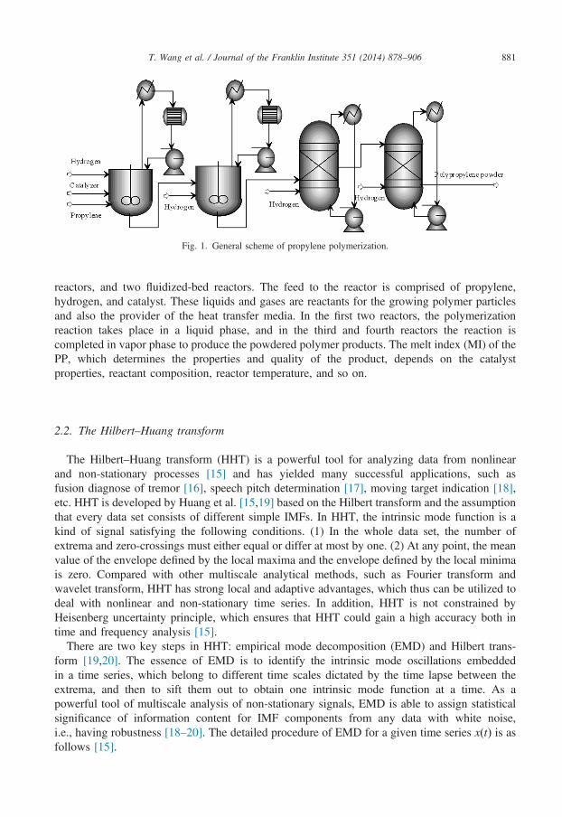
Fig. 1. General scheme of propylene polymerization.


reactors, and two fluidized-bed reactors. The feed to the reactor is comprised of propylene,hydrogen, and catalyst. These liquids and gases are reactants for the growing polymer particlesand also the provider of the heat transfer media. In the first two reactors, the polymerizationreaction takes place in a liquid phase, and in the third and fourth reactors the reaction iscompleted in vapor phase to produce the powdered polymer products. The melt index (MI) of thePP, which determines the properties and quality of the product, depends on the catalystproperties, reactant composition, reactor temperature, and so on.

2.2. The Hilbert–Huang transform

The Hilbert–Huang transform (HHT) is a powerful tool for analyzing data from nonlinearand non-stationary processes [15] and has yielded many successful applications, such asfusion diagnose of tremor [16], speech pitch determination [17], moving target indication [18],etc. HHT is developed by Huang et al. [15,19] based on the Hilbert transform and the assumptionthat every data set consists of different simple IMFs. In HHT, the intrinsic mode function is akind of signal satisfying the following conditions. (1) In the whole data set, the number ofextrema and zero-crossings must either equal or differ at most by one. (2) At any point, the meanvalue of the envelope defined by the local maxima and the envelope defined by the local minimais zero. Compared with other multiscale analytical methods, such as Fourier transform andwavelet transform, HHT has strong local and adaptive advantages, which thus can be utilized todeal with nonlinear and non-stationary time series. In addition, HHT is not constrained byHeisenberg uncertainty principle, which ensures that HHT could gain a high accuracy both intime and frequency analysis [15].

There are two key steps in HHT: empirical mode decomposition (EMD) and Hilbert trans-form [19,20]. The essence of EMD is to identify the intrinsic mode oscillations embeddedin a time series, which belong to different time scales dictated by the time lapse between theextrema, and then to sift them out to obtain one intrinsic mode function at a time. As apowerful tool of multiscale analysis of non-stationary signals, EMD is able to assign statisticalsignificance of information content for IMF components from any data with white noise,i.e., having robustness [18–20]. The detailed procedure of EMD for a given time series xðtÞ is asfollows [15].


In this process, i, j, k are the counting unit, cjðtÞ are the IMFs, rjðtÞ are the residual series andhiðtÞ are the iterative transition sequences.

(1)
Take the signal xðtÞ for example and identify all the local extreme a of xðtÞ. (2) Connect all of the local maxima by a cubic spline line as the upper envelope emaxðtÞ. Repeat
the procedure for the local minima to produce the lower envelope eminðtÞ.
(3) Calculate the mean value m1ðtÞ of upper and lower envelopes, that is
m1ðtÞ ¼ ðemaxðtÞ þ eminðtÞÞ=2 ð1Þ
(4) Subtract m1ðtÞ from original signal, named as h1ðtÞ: h1ðtÞ ¼ xðtÞ�m1ðtÞ. Judge whether h1ðtÞ
satisfies IMF conditions or not, if so, then as the first IMF it is denoted as c1ðtÞ ¼ h1ðtÞ; if not,replace xðtÞ with h1ðtÞ, and then calculate h11ðtÞ ¼ h1ðtÞ�m11ðtÞ, where m11ðtÞ is the mean ofthe upper and lower envelopes of h1ðtÞ. This process can be repeated up to k times, untilh1kðtÞ satisfies IMF conditions, then the first IMF component from the data is designated asc1ðtÞ ¼ h1kðtÞ.

(5)
Once c1ðtÞ is obtained, it can be separated from the rest of the data by using
xðtÞ�c1ðtÞ ¼ r1ðtÞ ð2Þ
(6) Repeat steps (1) to (5) using r1ðtÞ as xðtÞ to obtain c2ðtÞ until rnðtÞ is a monotone function or a
direct current component. That is

r1ðtÞ�c2ðtÞ ¼ r2ðtÞ…rn�1ðtÞ�cnðtÞ ¼ rnðtÞ: ð3Þ
(7) By summing up Eqs. (2) and (3), we finally obtain
xðtÞ ¼ ∑n

j ¼ 1cjðtÞ þ rnðtÞ ð4Þ

To guarantee that each IMF component retains enough physical sense of amplitude andfrequency modulations, the sifting process can be accomplished by limiting the size of thestandard deviation (SD), computed from the two consecutive sifting results as

SD¼ ∑T

t ¼ 0½jhiðtÞ�hi�1ðtÞj2=h2i�1ðtÞ�oε ð5Þ

where ε is closed as 0.2 in PP progress, and the values lie between 0.2 and 0.3 in the study.The second step of HHT is to apply Hilbert transform on each decomposed signal, which is

defined as

yjðtÞ ¼ cjðtÞn1πt

¼ 1πPV

Z þ1

�1½cjðt′Þ=ðt� t′Þ�dt′ ð6Þ

where PV represents the principal value of the singular integral. Then the analytic signal isobtained as follows:

zjðtÞ ¼ cjðtÞ þ iyjðtÞ ¼ ajðtÞeiφjðtÞ ð7Þwhere ajðtÞ is the instantaneous amplitude and φjðtÞ is the phase function satisfying

ajðtÞ ¼ffiffiffiffiffiffiffiffiffiffiffiffiffiffiffiffiffiffiffiffiffiffiffiffic2j ðtÞ þ y2j ðtÞ

qtan φjðtÞ ¼ yjðtÞ=cjðtÞ

8<: ð8Þ


The instantaneous frequency ωjðtÞ is the time derivative of φjðtÞ, i.e.,ωjðtÞ ¼ dφjðtÞ=dt ð9Þ

Finally, the original series can be expressed as follows:

xðtÞ ¼ Re ∑n

j ¼ 1ðajðtÞei

RωjðtÞdtÞ ð10Þ

The residual is left out on purpose, for it is either a monotonic function or a constant.However, while the residue is monotonic or constant, the energy involved in the residual trendcould be overwhelming [15].

2.3. Lempel–Ziv complexity

Lempel–Ziv (LZ) complexity, advocated by Lempel and Ziv [21–24], is a popular metric forcharacterizing time series and shows high effectiveness in entropy estimation from short dataintervals [29]. In the current paper, the extensively popular LZ algorithm [22] proposed in 1976is used. The detailed procedure for calculating the LZ complexity is as follows [22].

(i)
The numerical series x¼ fx1; x2; :::; xng has to be first transformed into a symbolicsequence. One popular approach is to convert the signal into a 0–1 sequenceS¼ fs1; s2; :::; sng with a threshold value x, where si ¼ 1, if xi4x, otherwise si ¼ 0.Usually, x is chosen to be the median of x.
(ii)
Define the substring
Sðp; qÞ ¼sp; spþ1; :::; sq; prq

∅; p4q

(ð11Þ

and VðSÞ to be the vocabulary of a sequence S. Namely, VðSÞ is a set of all the substring ofthe sequence S. For example, let S¼010, then VðSÞ ¼ f0; 1; 01; 10; 010g. Initialize that i¼ 1,j¼ 1 and the number of inserted dots is com ðnÞ ¼ 0.

(iii)
Compare the substring Sði; jÞ to VðSð1; j�1ÞÞ. If Sði; jÞ has already consisted inVðSð1; j�1ÞÞ, then update i¼ i and j¼ jþ 1; else update i¼ iþ 1, j¼ jþ 1 andcom ðnÞ ¼ com ðnÞ þ 1.
(iv)
Repeat step (iii) until j¼ n. (v) Finally, place a dot after the last element sn and update com ðnÞ ¼ com ðnÞ þ 1. (vi) Calculate the Lempel–Ziv complexity by
COM ðnÞ ¼ com ðnÞðlog 2ðnÞ þ 1Þ=n ð12Þ

2.4. Time-delay embedding technique and G–P algorithm

Time-delay embedding technique provides an effective method to diagnose the nonlineardynamics behavior of a system from a time series [8]. For a set of observable signals fxig,i¼ 1; 2; :::;N; the reconstructed patterns

Xi ¼ ½xi; xiþτ; :::; xiþðm�1Þτ�; i¼ 1; 2; :::;Nm ð13Þ


are thought to be able to trace out the orbit of the studied nonlinear dynamical system. Here, τ isthe time delay, m is the embedding dimension and Nm ¼ N�ðm�1Þτ is the size of the vectorpoints. The typical condition is m5N and τ40. Generally, τ and m are two key parameters in thereconstruction process which should be chosen with caution. There are many methods reportedto estimate τ and m, like mutual information [25,26] for τ and G–P algorithm [13] for m, etc.Mutual information [25] is a classical method to estimate the time delay τ and the algorithm canbe found in a series of literatures [13,25,26]. Mutual information is an information theoryproperty launched from the angle of entropy (average information). The Mutual informationbetween xðtÞ and xðt þ τÞ is defined as

IðτÞ ¼ ∑xðtÞ;xðtþτÞ

PðxðtÞ; xðt þ τÞÞlog 2PðxðtÞ; xðt þ τÞÞPðxðtÞÞPðxðt þ τÞÞ

� �ð14Þ

where PðxðtÞÞ is the normalized distribution of xðtÞ, Pðxðt þ τÞÞ is the normalized distribution ofxðt þ τÞ, and PðxðtÞ; xðt þ τÞÞ is the simultaneous distribution. A good practical habit of selectionis the first minimum value of IðτÞ.A classical algorithm to estimate D2 was put forward by Grassberger and Procaccia, which is

called G–P algorithm. Here we give a detailed description of the G–P algorithm [13]. Thecorrelation integral is defined as

CðrÞ ¼ 2NmðNm�1Þ ∑

1r ir jrNm

Hðr�jXi�XjjÞ; ð15Þ

where r is the selected radius and HðxÞ is the Heaviside function,

HðxÞ ¼1; x40

0; xr0

(ð16Þ

if the studied system is chaotic, there is an exponential law between C(r) and r acting as

CðrÞprD2ðmÞ ð17Þwhere D2ðmÞ is the correlation dimension. It may be estimated from the slop and intercept of thecurve between ln CðrÞ versus ln r in a linear scaling region.In the process of applying G–P algorithm to real data, it should be noted that G–P algorithm

usually needs large-scale data set while the length of real data is often finite. To verify thevalidity of G–P algorithm in practical application, some formulas are proposed to estimate themaximum embedding dimension which can be supported by the size of real data [27,28]. If theestimated values of m are beyond the maximum estimation, the result of the G–P algorithmapplication is questionable. Therefore, the following formula is used to verify the validity of thiswork in the subsequent investigation

m5ffiffiffiffiN

pn ð“failure rate”Þ2=“normalized dynamic noise variance”; ð18Þ

where “normalized dynamic noise variance”¼var(noise)/var(sample).Next the false nearest method to select the best embedding dimension will be introduced. The

nearest approach relies on the geometry of the embedded theorem: with the increase of thedimension, the attractor will be launched. On the rail line, the seemingly close point in ddimension space would be apart in the dþ1 dimension space and the point is the ‘false’ neighborpoint in the d dimension space. This method is used to estimate the percentage of ‘false’ neighborpoints when the dimension increases. The neighbor point of s(k) in the d�1 dimension space is


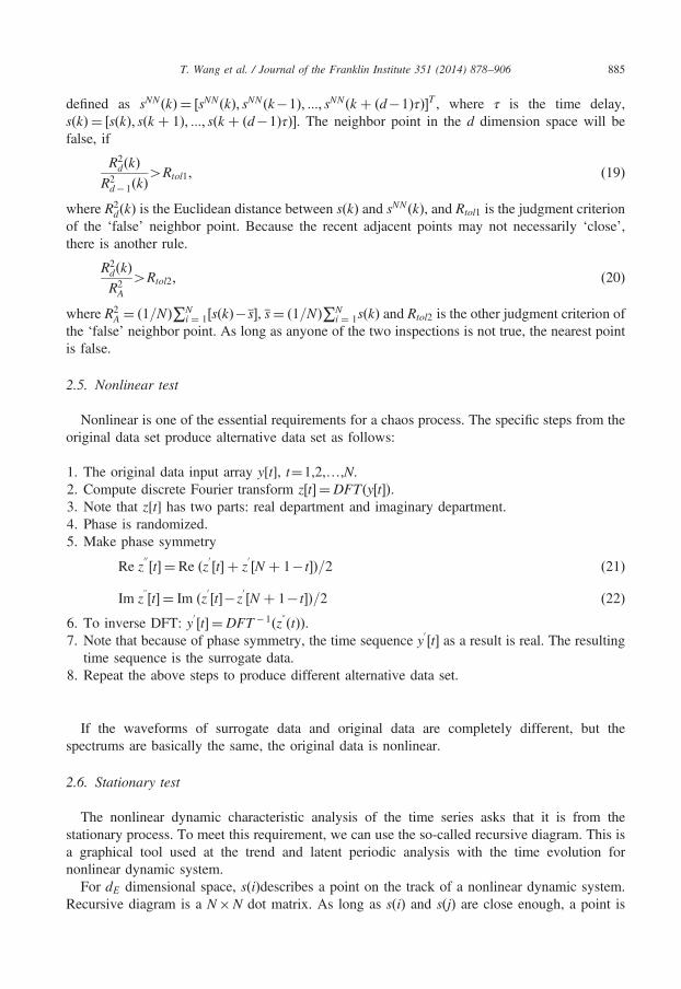
defined as sNNðkÞ ¼ ½sNNðkÞ; sNNðk�1Þ; :::; sNNðk þ ðd�1ÞτÞ�T , where τ is the time delay,sðkÞ ¼ ½sðkÞ; sðk þ 1Þ; :::; sðk þ ðd�1ÞτÞ�. The neighbor point in the d dimension space will befalse, if

R2dðkÞ

R2d�1ðkÞ

4Rtol1; ð19Þ

where R2dðkÞ is the Euclidean distance between sðkÞ and sNNðkÞ, and Rtol1 is the judgment criterion

of the ‘false’ neighbor point. Because the recent adjacent points may not necessarily ‘close’,there is another rule.

R2dðkÞR2A

4Rtol2; ð20Þ

where R2A ¼ ð1=NÞ∑N

i ¼ 1½sðkÞ�s�, s¼ ð1=NÞ∑Ni ¼ 1sðkÞ and Rtol2 is the other judgment criterion of

the ‘false’ neighbor point. As long as anyone of the two inspections is not true, the nearest pointis false.

2.5. Nonlinear test

Nonlinear is one of the essential requirements for a chaos process. The specific steps from theoriginal data set produce alternative data set as follows:

1.
The original data input array y[t], t¼1,2,…,N. 2. Compute discrete Fourier transform z½t� ¼DFTðy½t�Þ. 3. Note that z[t] has two parts: real department and imaginary department. 4. Phase is randomized. 5. Make phase symmetry
Re z00 ½t� ¼Re ðz0 ½t� þ z

0 ½N þ 1� t�Þ=2 ð21Þ

Im z}½t� ¼ Im ðz0 ½t��z0 ½N þ 1� t�Þ=2 ð22Þ

6.
To inverse DFT: y0 ½t� ¼DFT �1ðz}ðtÞÞ.
7.
Note that because of phase symmetry, the time sequence y0 ½t� as a result is real. The resulting
time sequence is the surrogate data.
8. Repeat the above steps to produce different alternative data set.
If the waveforms of surrogate data and original data are completely different, but thespectrums are basically the same, the original data is nonlinear.

2.6. Stationary test

The nonlinear dynamic characteristic analysis of the time series asks that it is from thestationary process. To meet this requirement, we can use the so-called recursive diagram. This isa graphical tool used at the trend and latent periodic analysis with the time evolution fornonlinear dynamic system.

For dE dimensional space, sðiÞdescribes a point on the track of a nonlinear dynamic system.Recursive diagram is a N�N dot matrix. As long as sðiÞ and sðjÞ are close enough, a point is


painted at the place ði; jÞ in lattice. In order to get a recursive diagram from a time series, in fact,we can make the following treatment:

(i)
Choose an embedding dimension dE and construct a dE dimension orbit by the delay. (ii) Choose rðiÞ to make a ball with sðiÞ as the center, rðiÞ as the radius, which contains the
appropriate number of other points in the orbit.
(iii) For every point sðjÞ is located in the ball, a point is painted at the place ði; jÞ in the graph.
This graph is called recursive diagram. Note that i; j is the unit of time to measure and the chartis quite symmetrical about diagonal i¼ j. We couldn't expect to get a completely symmetricalfigure. The more symmetrical the graph is, the stronger the stability is.

2.7. Maximum Lyapunov exponent

Lyapunov exponents measure the average exponent rate of divergence or convergence of nearbytrajectories in phase space. Compared with correlation dimension, Lyapunov exponents can providea more useful characterization of chaos [29]. Among all the Lyapunov exponents of a system, themaximum Lyapunov exponent (MLE), denoted as λ1, is the most concerned about. Different λ1 canindicate different type of motion of a system [29]: (a) λ1o0 means stable fixed point; (b) λ1 ¼ 0means stable limit cycle; (c) 0oλ1o1 means chaos; (d) λ1 ¼1 means randomicity. There aremany methods reported to estimate Lyapunov exponents from a time series [30–32]. In the currentstudy, the algorithm provided by Wolf et al. [30] is chosen to estimate the MLE.

2.8. Algorithms of detecting interdependences

As is well known, nonlinear interactions induce dissipative structures [33]. It is very importantto quantify the interactions for more accurate modeling. There are many reported methods forinference of coupling in nonlinear system, such as the dimension of interaction dynamics [14],the robust method for detecting interdependences [34], characterization of synchrony [35], phasesynchrony [36], etc. Here, for the simplicity sake, the first two algorithms are placed specialattention in the subsequent research. Besides, the dimension of interaction dynamics is a usefulmeasure to determine whether two chaotic series originate from two interaction or non-interaction systems, or to quantify the common part of chaotic dynamics when they come fromcoupling systems. Successful application of this method is realized on the data from coupledHennon maps and logistic maps [14]. The detailed algorithm about this is described below.Suppose xaðtÞ and xbðtÞ are time series from two subsystems and construct a new function of

xaðtÞ and xbðtÞ, xab ¼ f ðxaðtÞ; xbðtÞÞ. In the current work, this new function is chosen to bexab ¼ xaðtÞ þ xbðtÞ for convenience. The dimension of interaction dint2 is given by

dint2 ¼D2ðxaðtÞÞ þ D2ðxbðtÞÞ�D2ðxabðtÞÞ ð23Þlet

m2a ¼ dint2 =D2ðxaðtÞÞ

m2b ¼ dint2 =D2ðxbðtÞÞ

m2ab ¼ dint2 =D2ðxabðtÞÞ

8><>: ð24Þ


if m2i a0, these variables satisfy

1m2

a

þ 1m2

b

� 1m2

ab

¼ 1 ð25Þ

here, m2a, m

2b, and m2

ab represent the generalized dimension. There are four nonequivalent casesfor a coupling system [14]:

Case 1: m2a ¼m2

b ¼m2ab ¼ 0 (no interaction).

Case 2: 1¼m2a ¼m2

b ¼m2ab (maximal coupling: xa ¼ xb ¼ xab).

Case 3: 1¼m2a4m2

b ¼m2ab40 (all degrees of freedom of xa couple to some variables of xb, or

xa is the driver in the pair, which gives xb ¼ xab).Case 4: 14m2

aZm2b4m2

ab40 (interaction or double control).

It should be noted that the dimension of interaction dynamics is suitable for quantifyingnonlinear interdependence of two series when they are both chaotic [14].

Another robust method for detecting interdependences is proposed by Arnhold [34], which isnon-symmetric and can provide information about the direction of driving even if theinterpretation in terms of causal relations is not straightforward [34]. For the above two timeseries: xa and xb, this method is constructed as follows [34].

(i)
According to Eq. (13), reconstruct xa and xb to be Xan ¼ ðxan; :::; xaðn�ðm1�1Þτ1ÞÞ, Xbn ¼ðxbn; :::; xbðn�ðm1�1Þτ1ÞÞ respectively.
(ii)
Use mutual information technique [25] and algorithm [11] to estimate the reconstructedparameters in step (i).
(iii)
Define the following measures for these two series
RðkÞn ðxaÞ ¼

1k∑k

j ¼ 1ðXan�Xarn;j Þ2 ð26Þ

RðkÞn ðxbÞ ¼

1k∑k

j ¼ 1ðXbn�Xbsn;jÞ2 ð27Þ

where rn;j, sn;j denote the time indices of the jth nearest neighborhood point of Xan and Xbn,respectively, and k represents the number of nearest neighbor points.

(iv)
Based on Eqs. (26) and (27), define the conditional measures of two time series as
RðkÞn ðxajxbÞ ¼

1k∑k

j ¼ 1ðXan�Xasn;jÞ2 ð28Þ

RðkÞn ðxbjxaÞ ¼

1k∑k

j ¼ 1ðXbn�Xbrn;j Þ2 ð29Þ

(v)
At last, define local and global interdependence measures SknðxajxbÞ and SðkÞðxajxbÞ asSknðxajxbÞ ¼ RðkÞ
n ðxaÞ=RðkÞn ðxajxbÞ ð30Þ

SðkÞðxajxbÞ ¼1N

∑N

i ¼ 1SðkÞn ðxajxbÞ ð31Þ


Analogously, we can define SnðxbjxaÞ and S ðxbjxaÞ. Since SnðxajxbÞZSn ðxaÞ, we have0oSðkÞðxajxbÞr1. There are three cases to characterize the coupling of these two series.

k ðkÞ k ðkÞ

(1)
If SðkÞðxajxbÞ51, xa is independent of xb within the limits of accuracy. (2) If SðkÞðxajxbÞ-1, the dependence of xa on xb becomes maximal. (3) If SðkÞðxajxbÞ4SðkÞðxbjxaÞ, the dependence of xa on xb is stronger than that of xb on xa.
In general, it is a difficult task to measure the coupling in nonlinear systems. Here, twomethods are introduced for this task. The main motivation is to verify whether the inference ofcoupling between the different methods is consistent.

3. Results and discussion

3.1. Data set

In the current work, the time series of the melt index collected from a real propylenepolymerization process, is selected as the sample set, with the size of the time series 85, which islong enough for performing a general nonlinear analysis, and the sampling interval about 2 h.Fig. 2 illustrates the melt index time series. The x axis is the number of samples and the y axis

is the melt index value. In this curve, there are a lot of irregular troughs and waves. Obviously,complex oscillations and irregular behaviors can be observed in the figure.According to the theory of Section 2.5 Nonlinear test, we can produce the surrogate data.

Fig. 3 represents the data and the spectrum of the original data and the surrogate data. The leftfigure is the data of the original data and the surrogate data. The x axis is the number of samplesand the y axis is the melt index value. The right figure is the spectrum of the original data and thesurrogate data. The x axis is the number of samples and the y axis is the spectrum value. From

Fig. 2. The time series of the melt index (MI) in the propylene polymerization industry.


Fig. 3, the waveforms of surrogate data and original data are completely different, but thespectrums are basically the same, so the original data is nonlinear.

According to the theory of Section 2.6 Stationary test, we can attain the recursive diagram.Fig. 4 is the recursive diagram of the original data. From Fig. 4, we can see that the graph issymmetrical, so the stability of the data is strong. Thus, the melt index is nonlinear and stable.

3.2. Multiscale analysis and complexity measure

Applications of EMD method in the Section 2.2 The Hilbert–Huang transform to the meltindex series produce three IMFs and the residual, shown in Fig. 5, respectively. The x axis is thenumber of samples and the y axis is the melt index value. In the figure, c1, c2, c3 are the threeIMFs and r3 is the residual. Generally, the number of IMFs depends on the stopping criteria(Eq. (5)) and experimental conditions. In the studied case, the experimental conditions aredefinite, so the stopping criteria, i.e., the threshold of ε, will have an effect on the number ofIMFs. Huang et al. [15] suggest that ε between [0.2, 0.3] is appropriate. Here, a routine valueε¼ 0:2 is selected as the stopping criteria to perform EMD on the MI time series. It is worthpointing out that the EMD is a method by which a complicated signal can be expressed by a sumof proper rotations (if possible). As a consequence of the EMD, the complex plane of the analyticsignal constructed from each IMF exhibits a preferred direction of rotation (either clockwise orcounterclockwise) and the rotation can be defined with respect to a unique center [14,37].

The phase functions (φiðtÞ, i¼ 1; 2; 3) of the IMFs are shown in Fig. 6. The x axis is the numberof samples and the y axis is the angle value. From Fig. 6, we can see that the phase functions aresimilar and almost coincidence. So, the three IMFs are equally important and no one can be ignored.

Fig. 3. The data and the spectrum of the original data and the surrogate data.

Fig. 4. The recursive diagram of the original data.

Fig. 5. The IMFs and the residue for the studied MI time series shown in Fig. 2 through the empirical modedecomposition method.


The averaged instantaneous frequencies (wmean) and LZ complexity (COM) for each IMF obtainedfrom the studied MI time series are shown in Table 1. From Table 1, we can see that the averagedinstantaneous frequencies of three IMFs and r3 are 0.43, 0.314, 0.316 and 0.055, respectively. It can befound that, for the time series, the average instantaneous frequencies of the IMFs are almost the same.

Fig. 6. Phase function of each IMF decomposed from the studied MI time series.

Table 1Averaged instantaneous frequencies (wmean), LZ complexity (COM) for each IMF obtained from the studied MI timeseries.

P Original IMF(1) IMF(2) IMF(3) r3

wmean – 0.43 0.314 0.316 0.055COM 5.8403 6.5377 3.0500 5.7532 3.6611


The distribution of averaged instantaneous frequency indicates that IMF(1) extracts most random partof the original signal and IMF(2)–IMF(3) contain mostly deterministic components. These qualitativeresults may be further verified in the following analysis. From Table 1 we can get the LZ complexitycorresponding to the original signal, each IMF and r3 are 5.8403, 6.5377, 3.0500, 5.7532 and 3.6611.It can be seen that the IMF(1) of the time series has higher LZ complexity than the correspondingoriginal series, while the complexity of other IMFs is lower than that of the original signal (6.5377(IMF(1))45.8403(the original signal)45.7532(IMF(3))43.6611(r3)43.0500(IMF(2))). It is apparent fromthis table that for the IMFs of series, the IMFs(1)–(3) of the melt index series with similar averagedinstantaneous frequencies and proximate contribution to the whole series are left and should be madefurther analysis to detect the possible nonlinear dynamics contained in them. To this task, attention isturned below.

3.3. Nonlinear dynamic analysis of subscale structures

G–P algorithm is a frequently used method to estimate the embedding dimension, correlationdimension, so as to detect the possible nonlinear dynamics contained in a real system. Accordingto Eqs. (12)–(15), the delay time should be determined before using G–P algorithm. Here,mutual information technique [25] is utilized to estimate the optimal of the original and IMFs(1)–(3). Figs. 7–10 show that the x axis is the time delay, and the y axis is mutual information


value. These curves show that the mutual information changes with the increase of embedding delayand the corresponding delay of the first minimum value of the curve is the embedding delay. From theFigs. 7–10, the time delay of the original series and the three IMFs are 2, 4, 5 and 6, correspondingly.With the time delay obtained, G–P algorithm is then applied to these IMFs and the results of ln CðrÞversus ln r are shown in Figs. 11–14. The x axis is the ln r and the y axis is the ln CðrÞ. It is clear thatthere is non-scale interval where the slope tends to be stable in each curve of Figs. 11–14. According toEq. (17), these stable slopes and the corresponding intercepts can be used to estimate the correlationdimension. If the estimated correlation dimension D2 for an IMF saturates with increasing embeddingdimension m, the fractal scaling exists in the plots of ln CðrÞ versus ln r of this IMF, and the plateauestimated value D2 is taken as the correlation dimension D2 of this IMF [14]. To avoid the subjectivity

Fig. 7. Mutual information figure of original.

Fig. 8. Mutual information figure of IMF(1).




in judging the existence of fractal scaling by observing the plots of ln CðrÞ versus ln r in Fig. 8 with theunaided eyes, the plots of D2ðrÞ versus ln r should be made. From G–P algorithm [11] and Eq. (17),the relationship between D2ðrÞ and ln r is

D2ðrÞ ¼d½ ln CðrÞ�d½ ln r� ð32Þ

where d½�=d½� means derivative and can be approximated by Δ½ ln CðrÞ�=Δ½ ln r�. Here, Δf ðrÞ �f ðr þ 1Þ� f ðrÞ. Therefore, the plots of D2ðrÞ versus ln r of the first three IMFs of the studied meltindex series are easily made by using the difference instead of derivative.

Fig. 11. ln C(r)-ln r curves of original MI time series with different embedding dimensions m.

Fig. 12. ln C(r)-ln r curves of IMF(1) with different embedding dimensions m.


Shown in Figs. 15–18 are the results. The x axis is the ln r and the y axis is the D2ðrÞ. It is clearfrom Figs. 15–18 that there are plateau regions for IMF(1)–IMF(3) obtained from the studiedseries, which means that the correlation dimension of the IMFs can be defined.To further diagnose whether there is an indicator to render chaos in IMFs(1)–(3) of the studied

series, the numerical values of D2 are evaluated with the results shown in Figs. 19–22 andTable 2. The x axis is the embedding dimension and the y axis is the D2. From Figs. 19–22, thecorresponding dimension of the stability of the curve is the correlation dimension and they are1.57, 1.06, 2.55 and 1.95, correspondingly.




According to Section 2.4 time-delay embedding technique and G–P algorithm, we can attainthe embedding dimension figure of original and IMFs(1)–(3). Figs. 23–26 shows the embeddingdimension figure of original and IMFs(1)–(3). The x axis is the embedding dimension and the yaxis is the percentage of ‘false’ neighbor points. From Figs. 23–26, the corresponding dimension,which the percentage of ‘false’ neighbor points is 0, is the embedding dimension and they are 5,3, 17 and 15, correspondingly. Obviously, the correlation dimensions of IMFs(1)–(3) of thestudied series reach saturation values when the embedding dimensions are greater than a certainvalue. Hence, the above results of the G–P algorithm application are conditionally believable.

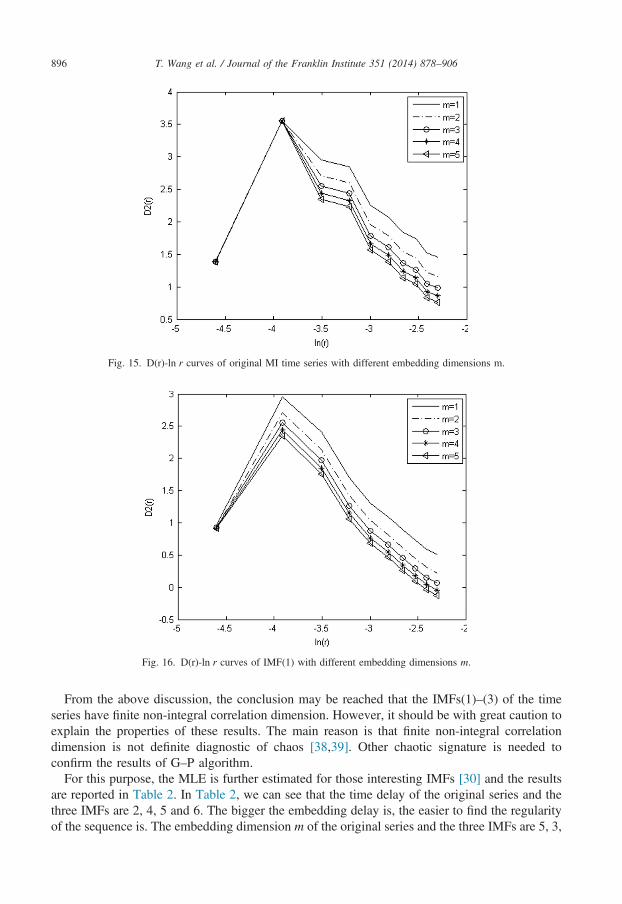
Fig. 15. D(r)-ln r curves of original MI time series with different embedding dimensions m.

Fig. 16. D(r)-ln r curves of IMF(1) with different embedding dimensions m.


From the above discussion, the conclusion may be reached that the IMFs(1)–(3) of the timeseries have finite non-integral correlation dimension. However, it should be with great caution toexplain the properties of these results. The main reason is that finite non-integral correlationdimension is not definite diagnostic of chaos [38,39]. Other chaotic signature is needed toconfirm the results of G–P algorithm.For this purpose, the MLE is further estimated for those interesting IMFs [30] and the results

are reported in Table 2. In Table 2, we can see that the time delay of the original series and thethree IMFs are 2, 4, 5 and 6. The bigger the embedding delay is, the easier to find the regularityof the sequence is. The embedding dimension m of the original series and the three IMFs are 5, 3,




17 and 15. Similar, the bigger the embedding dimension is, the easier to find the regularity of thesequence is. The correlation dimension D2 of the original series and the three IMFs are 1.57,1.06, 2.55 and 1.95 and they are fractional dimension, which show that they may be chaoticsequence. The maximum Lyapunov exponent of the original series and the three IMFs are0.1430, 1.0685, 0.2499 and þ1. It is clear that the IMF(3) of the series is random due toλ1 ¼1, and the IMFs(1)–(2) of the series are chaotic due to existence of positive finite MLE.In conclusion to this, the finite non-integral correlation dimension and the positive finite MLE forIMFs(1)–(2) of the studied series render a strong indicator that there is a chaotic mechanismgoverning the nonlinear dynamics of PP system. The analytic results on the IMF(3) of the studied

Fig. 19. The change of correlation dimension of original as embedding dimension changes.

Fig. 20. The change of correlation dimension of IMF(1) as embedding dimension changes.


series show that there is also a stochastic mechanism contained in PP system. Furthermore, thesetwo kinds of mechanism govern different sublevel structures of PP system, i.e., randommechanism governing the structures with a smaller size while chaotic mechanism governing thestructures with a larger structure. A chaotic multiscale feature is quite evident in PP system.In summary, multiscale feature and multiple dynamics are diagnosed in PP system through

combining EMD method with chaotic analysis. So, the melt index series is a very complicatedsignal and it often poses a great challenge to predict the product's property and qualitycontrolling of practical industrial process. Multiscale method can provide an alternative tool forMI prediction, such as chaotic model for sublevel structures with larger size and random model



Table 2Time delay, embedding dimension m, correlation dimension D2, and the maximum Lyapunov exponent of the three IMFsobtained from the studied time series.

P Original IMF(1) IMF(2) IMF(3)

Time delay 2 4 5 6Embedding dimension m 5 3 17 15Correlation dimension D2 1.57 1.06 2.55 1.95The maximum Lyapunov exponent 0.1430 1.0685 0.2499 –


Fig. 23. The embedding dimension figure of original.

Fig. 24. The embedding dimension figure of IMF(1).


for sublevel structures with smaller size. In this regard, it is meaningful to investigate melt indexseries using EMD method and chaotic analysis. However, it should be noted that it is not verymeaningful to combine the EMD method with chaotic analysis for purely chaotic signal orrandom signal, since chaotic signatures can be easily destroyed by filtering [40] and the IMFs ofrandom signal may possess certain structures. For all this, it does not hinder the application ofcombining EMD method and chaotic analysis to melt index series, because the melt index seriesis neither purely chaotic nor purely random signal according to the above research results.Therefore, it is meaningful to investigate melt index series using the EMD method and chaoticanalysis.




3.4. Multiscale coupling analysis

The above analysis on the studied melt index series through Lempel–Ziv complexity [24],G–P algorithm [13], and MLE [27] indicates that it will become easier and more pertinent todescribe IMFs(1)–(2) than the original signal, since low Lempel–Ziv complexity and definitenonlinear dynamics are found in the most interesting IMFs(1)–(2). Therefore, multiscaleresolution on PP system has potential to reduce the complexity for modeling, control andoptimization of PP system. Of course, a PP system is not just the sum of all its subscale structuresand there is also strong coupling between the subscale structures of PP system. The complex

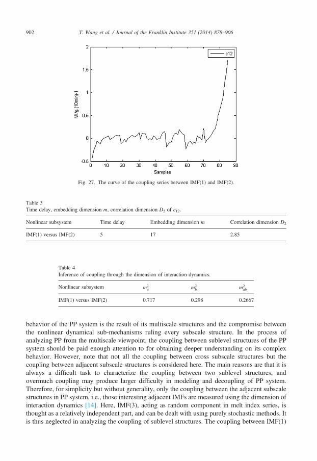
Fig. 27. The curve of the coupling series between IMF(1) and IMF(2).

Table 3Time delay, embedding dimension m, correlation dimension D2 of c12.

Nonlinear subsystem Time delay Embedding dimension m Correlation dimension D2

IMF(1) versus IMF(2) 5 17 2.85

Table 4Inference of coupling through the dimension of interaction dynamics.

Nonlinear subsystem m2a m2

b m2ab

IMF(1) versus IMF(2) 0.717 0.298 0.2667


behavior of the PP system is the result of its multiscale structures and the compromise betweenthe nonlinear dynamical sub-mechanisms ruling every subscale structure. In the process ofanalyzing PP from the multiscale viewpoint, the coupling between sublevel structures of the PPsystem should be paid enough attention to for obtaining deeper understanding on its complexbehavior. However, note that not all the coupling between cross subscale structures but thecoupling between adjacent subscale structures is considered here. The main reasons are that it isalways a difficult task to characterize the coupling between two sublevel structures, andovermuch coupling may produce larger difficulty in modeling and decoupling of PP system.Therefore, for simplicity but without generality, only the coupling between the adjacent subscalestructures in PP system, i.e., those interesting adjacent IMFs are measured using the dimension ofinteraction dynamics [14]. Here, IMF(3), acting as random component in melt index series, isthought as a relatively independent part, and can be dealt with using purely stochastic methods. Itis thus neglected in analyzing the coupling of sublevel structures. The coupling between IMF(1)

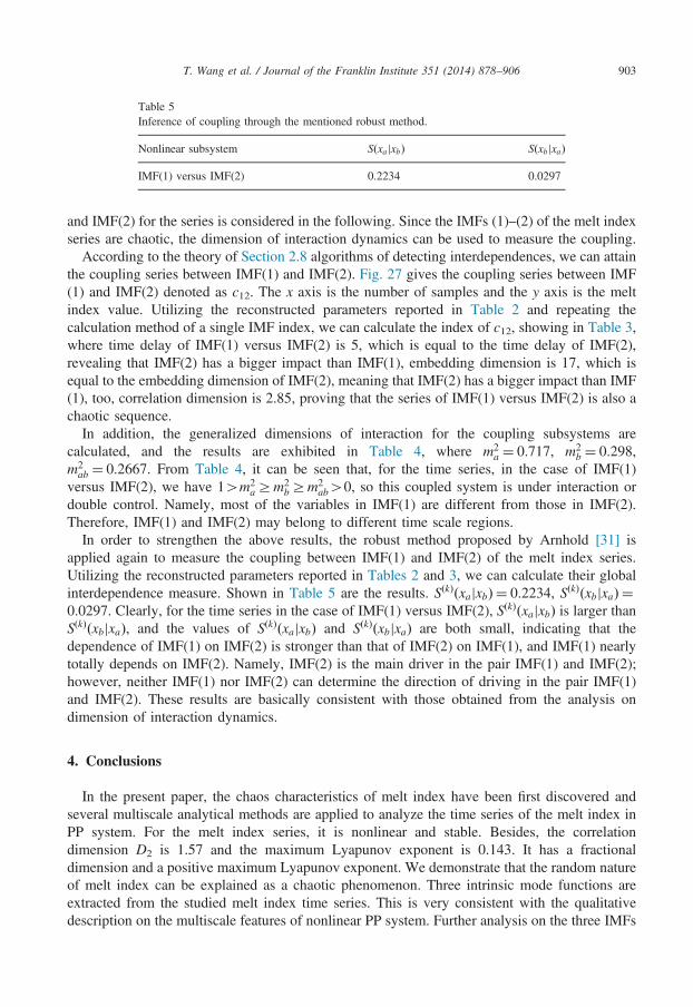
Table 5Inference of coupling through the mentioned robust method.

Nonlinear subsystem SðxajxbÞ SðxbjxaÞ

IMF(1) versus IMF(2) 0.2234 0.0297


and IMF(2) for the series is considered in the following. Since the IMFs (1)–(2) of the melt indexseries are chaotic, the dimension of interaction dynamics can be used to measure the coupling.

According to the theory of Section 2.8 algorithms of detecting interdependences, we can attainthe coupling series between IMF(1) and IMF(2). Fig. 27 gives the coupling series between IMF(1) and IMF(2) denoted as c12. The x axis is the number of samples and the y axis is the meltindex value. Utilizing the reconstructed parameters reported in Table 2 and repeating thecalculation method of a single IMF index, we can calculate the index of c12, showing in Table 3,where time delay of IMF(1) versus IMF(2) is 5, which is equal to the time delay of IMF(2),revealing that IMF(2) has a bigger impact than IMF(1), embedding dimension is 17, which isequal to the embedding dimension of IMF(2), meaning that IMF(2) has a bigger impact than IMF(1), too, correlation dimension is 2.85, proving that the series of IMF(1) versus IMF(2) is also achaotic sequence.

In addition, the generalized dimensions of interaction for the coupling subsystems arecalculated, and the results are exhibited in Table 4, where m2

a ¼ 0:717, m2b ¼ 0:298,

m2ab ¼ 0:2667. From Table 4, it can be seen that, for the time series, in the case of IMF(1)

versus IMF(2), we have 14m2aZm2

bZm2ab40, so this coupled system is under interaction or

double control. Namely, most of the variables in IMF(1) are different from those in IMF(2).Therefore, IMF(1) and IMF(2) may belong to different time scale regions.

In order to strengthen the above results, the robust method proposed by Arnhold [31] isapplied again to measure the coupling between IMF(1) and IMF(2) of the melt index series.Utilizing the reconstructed parameters reported in Tables 2 and 3, we can calculate their globalinterdependence measure. Shown in Table 5 are the results. SðkÞðxajxbÞ ¼ 0:2234, SðkÞðxbjxaÞ ¼0:0297. Clearly, for the time series in the case of IMF(1) versus IMF(2), SðkÞðxajxbÞ is larger thanSðkÞðxbjxaÞ, and the values of SðkÞðxajxbÞ and SðkÞðxbjxaÞ are both small, indicating that thedependence of IMF(1) on IMF(2) is stronger than that of IMF(2) on IMF(1), and IMF(1) nearlytotally depends on IMF(2). Namely, IMF(2) is the main driver in the pair IMF(1) and IMF(2);however, neither IMF(1) nor IMF(2) can determine the direction of driving in the pair IMF(1)and IMF(2). These results are basically consistent with those obtained from the analysis ondimension of interaction dynamics.

4. Conclusions

In the present paper, the chaos characteristics of melt index have been first discovered andseveral multiscale analytical methods are applied to analyze the time series of the melt index inPP system. For the melt index series, it is nonlinear and stable. Besides, the correlationdimension D2 is 1.57 and the maximum Lyapunov exponent is 0.143. It has a fractionaldimension and a positive maximum Lyapunov exponent. We demonstrate that the random natureof melt index can be explained as a chaotic phenomenon. Three intrinsic mode functions areextracted from the studied melt index time series. This is very consistent with the qualitativedescription on the multiscale features of nonlinear PP system. Further analysis on the three IMFs


of the time series using time-delay embedding, G–P algorithm, and MLE shows that IMF(3)extracts most of the random part in the original signal. While the correlation dimension D2 ofIMF(1) and IMF(2) are 1.06, 2.55 and the maximum Lyapunov exponent are 1.0685, 0.2499.IMFs(1)–(2) have strong indication of deterministic components due to the presence of non-integer fractal dimension and positive finite maximum Lyapunov exponent. So, the PP meltindex series are divided into two chaotic signals, a determined signal and a random signalrespectively. In addition, coupling between IMF(1) and IMF(2) is investigated by the dimensionof interaction dynamics and a robust method for detecting interdependence. The results indicatethat IMF(2) is the main driver in the coupling systems. All of these represent that as the studiedmelt index is concerned, multiscale theory and methods may provide potential ways to analyzeits complex nonlinear dynamics and may further offer more candidate tools to model and controlit in the future.Of course, it should be mentioned that the current results are just coming from a single case

study. A series of systematic measurements should be conducted before drawing any conclusionson the invention of the future control procedure for this PP system using multiscale methods.Also, it needs to be emphasized that, despite identifying multiscale features, nonlinear dynamicsof subscale structures, and the coupling of two adjacent subscale structures of the selected meltindex through combining Hilbert–Huang transform and the above used nonlinear analysismethods, there are still much work [41–53] needed to be done in the future to strengthen theresults obtained here. The corresponding work is ongoing.

Acknowledgments

This work is supported by Joint Funds of NSFC-CNPC of China (Grant U1162130), NationalHigh Technology Research and Development Program (863, Grant 2006AA05Z226) andZhejiang Provincial Natural Science Foundation for Distinguished Young Scientists (GrantR4100133), and their supports are thereby acknowledged.

References

[1] D. Cafagna, G. Grassi, On the simplest fractional-order memristor-based chaotic system, Nonlinear Dynamics 70 (2)(2012) 1185–1197.

[2] H.S. Yi, J.H. Kim, C. Han, J. Lee, S. Na, Plant wide optimal grade transition for an industrial high-densitypolyethylene plant, Industrial and Engineering Chemistry Research 42 (2003) 91–98.

[3] Y. Chen, X. Liu, Modeling mass transport of propylene polymerization on Ziegler–Natta catalyst, Polymer 46(2005) 9434–9442.

[4] H.Q. Jiang, Y. Xiao, J. Li, X.G. Liu, Prediction of the melt index based on the relevance vector machine withmodified particle swarm optimization, Chemical Engineering and Technology 35 (2012) 819–826.

[5] J. Shi, X.G. Liu, Melt index prediction by weighted least squares support vector machines, Journal of AppliedPolymer Science 101 (2006) 285–289.

[6] J. Li, X.G. Liu, H. Jiang, Y. Xiao, Melt index prediction by adaptively aggregated rbf neural networks trained withnovel ACO algorithm, Journal of Applied Polymer Science 125 (2012) 943–951.

[7] J. Li, X.G. Liu, Melt index prediction by RBF neural network optimized with an adaptive new ant colonyoptimization algorithm, Journal of Applied Polymer Science 119 (2011) 3093–3100.

[8 M. Zhang, X. Liu, A. Soft, Sensor based on adaptive fuzzy neural network and support vector regression forindustrial melt index prediction, Chemometrics and Intelligent Laboratory Systems 126 (2013) 83–90.

[9] X. Liu, J. Lu, Least squares based iterative identification for a class of multirate systems, Automatica 46 (2010)549–554.

http://refhub.elsevier.com/S0016-0032(13)00359-1/sbref1



















[10] Hagerty, R.O., Burdett, I.D., DeChellis, M.I., Method for on-line monitoring and control of polymerizationprocesses and reactors to prevent discontinuity events. US 2008/0319583 A1, 2007, pp. 1–16.

[11] Muhle, M.M., Nguyen, K., Finney, C., Daw, S., Method of applying non-linear dynamics to control a gas-phasepolyethylene reactor operability. WO 03/051929 A1, 2008, pp. 1–25.

[12] N.H. Packard, J.P. Crutchfield, J.D. Farmer, R.S. Shaw, Geometry from a time series, Physical Review Letters 45(1980) 712–716.

[13] P. Grassberger, I. Procaccia, Characterization of strange attractors, Physical Review Letters 50 (1983) 346–349.[14] D. Wójcik, A. Nowak, M. Kus, Dimension of interaction dynamics, Physical Review E 63 (2001) 036221–036236.[15] H. Huang, J.Q. Pan, Speech pitch determination based on Hilbert–Huang transform, Signal Processing 86 (2006)

792–803.[16] L.M. Ai, J. Wang, X.L. Wang, Multi-features fusion diagnosis of tremor based on artificial neural network and D–S

evidence theory, Signal Processing 88 (2008) 2927–2935.[17] C.J. Cai, W.X. Liu, J.S. Fu, Y.L. Lu, A new approach for ground moving target indication in foliage environment,

Signal Processing 86 (2006) 84–87.[18] P. Flandrin, G. Rilling, P. Goncalves, Empirical Mode Decomposition as a filter bank, IEEE Signal Processing

Letters 11 (2004) 112–114.[19] Z. Wu, N.E. Huang, A study of the characteristics of white noise using the empirical mode decomposition method,

Proceedings of the Royal Society of London. Series A 460 (2004) 1597–1611.[20] N.E. Huang, Z. Shen, The empirical mode decomposition and the Hilbert spectrum for nonlinear and non-stationary

time series analysis, Proceedings of the Royal Society of London. Series A 454 (1998) 903–995.[21] A. Lempel, J. Ziv, On the complexity of finite sequences, IEEE Transactions on Information Theory 22 (1976)

75–81.[22] A. Lempel, J. Ziv, Compression of individual sequences via variable-rate coding, IEEE Transactions on Information

Theory 24 (1978) 530–536.[23] X. Wu, Y. Lu, Generalized projective synchronization of the fractional-order Chen hyper chaotic system, Nonlinear

Dynamics 57 (2009) 25–35.[24] J.M. Amigo, J. Szczepanski, E. Wajnryb, M.V. Sanchez-Vives, Estimating the entropy rate of spike trains via

Lempel–Ziv complexity, Neural Computation 16 (2004) 717–736.[25] A.M. Fraser, H.L. Swinney, Independent coordinates for strange attractors from mutual information, Physical

Review A 33 (1986) 1134–1140.[26] R.Q. Quiroga, A. Kraskov, T. Kreuz, P. Grassberger, Performance of different synchronization measures in real

data: a case study on electroencephalographic signals, Physical Review E 65 (2002) 041903–041917.[27] D. Ruelle, Deterministic chaos:the science and the fiction, Proceedings of the Royal Society of London. Series A

427 (1990) 241–248.[28] B. Cheng, H. Tong, Orthogonal projection, embedding dimension and sample size in chaotic time series from a

statistical perspective [and discussion], Philosophical Transactions of the Royal Society of London. Series A 348(1994) 325–341.

[29] H. Kantz, T. Schreiber, Nonlinear Time Series Analysis, 2nd edition, Cambridge University Press, Cambridge,England, 2004.

[30] A. Wolf, J.B. Swift, H.L. Swinney, J.A. Vastano, Determining Lyapunov exponents from a time series, Physica D16 (1985) 285–317.

[31] J.P. Eckmann, S.O. Kamphorst, Liapunov exponents from time series, Physical Review A 34 (1986) 4971–4979.[32] R. Brown, P. Bryant, Computing the Lyapunov spectrum of a dynamical system from an observed time series,

Physical Review A 43 (1991) 2787–2806.[33] J.H. Li, J.Y. Zhang, W. Ge, X.H. Liu, Multi-scale methodology for complex systems, Chemical Engineering

Science 59 (2004) 1687–1700.[34] J. Arnhold, P. Grassberger, K. Lehnertz, C.E. Elgerand, A robust method for detecting interdependences: application

to intracranially recorded EEG, Physica D 134 (1999) 419–430.[35] Y.C. Lai, M.G. Frei, I. Osorio, L. Huang, Characterization of synchrony with applications to epileptic brain signals,

Physical Review Letters 98 (2007) 108102–108106.[36] L. Angelini, M.De. Tommaso, M. Guido, K. Hu, P.Ch. Ivanov, Steady-state visual evoked potentials and phase

synchronization in migraine patients, Physical Review Letters 93 (2004) 038103–038107.[37] R.Q. Quiroga, J. Arnhold, P. Grassberger, Learning driver-response relationships from synchronization patterns,

Physical Review E 61 (2000) 5142–5148.[38] A.R. Osborne, A. Provenzale, Finite correlation dimension for stochastic systems with power-law spectra, Physica D

35 (1989) 357–381.

http://refhub.elsevier.com/S0016-0032(13)00359-1/othref0005

























































[39] A. Provenzale, A.R. Osborne, R. Soj, Convergence of the K2 entropy for random noises with power law spectra,Physica D 47 (1991) 361–372.

[40] R. Badii, G. Broggi, B. Derighetti, M. Ravani, A dimension increase in filtered chaotic signals, Physical ReviewLetters 60 (1988) 979–982.

[41] M. Cencini, M. Falcioni, E. Olbrich, H. Kantz, A. Vulpiani, Chaos or noise: difficulties of a distinction, PhysicalReview E 62 (2000) 427–437.

[42] J.B. Gao, J. Hu, W.W. Tung, Y.H. Cao, Distinguishing chaos from noise by scale-dependent Lyapunov exponent,Physical Review E 74 (2006) 066204–066213.

[43] J. Sun, X. Liu, A novel APSO-aided maximum likelihood identification method for Hammerstein systems,Nonlinear Dynamics 73 (2013) 449–462.

[44] X. Liu, C. Zhao, Melt index prediction based on fuzzy neural network and PSO algorithm with online correctionstrategy, AIChE Journal 58 (2012) 1194–1202.

[45] M. Huang, X. Liu, J. Li, Melt index prediction by RBF neural network with an ICO–VSA hybrid optimizationalgorithm, Journal of Applied Polymer Science 126 (2012) 519–526.

[46] H. Han, L. Xie, F. Ding, X. Liu, Hierarchical least-squares based iterative identification for multivariable systemswith moving average noises, Mathematical and Computer Modelling 51 (2010) 1213–1220.

[47] F. Ding, G. Liu, X.P. Liu, Parameter estimation with scarce measurements, Automatica 47 (8) (2011) 1646–1655.[48] X.J. Wu, J. Li, G.R. Chen, Chaos in the fractional order unified system and its synchronization, Journal of the

Franklin Institute 345 (4) (2008) 392–401.[49] Y.X. Guo, W.H. Jiang, B. Niu, Bifurcation analysis in the control of chaos by extended delay feedback, Journal of

the Franklin Institute 350 (1) (2013) 155–170.[50] A. Oksasoglu, Q.D. Wang, Rank one chaos in a switch-controlled Chua's circuit, Journal of the Franklin Institute

347 (9) (2010) 1598–1622.[51] M. Liu, Y. Shi, F. Fang, Optimal power flow and PGU capacity of CCHP systems using a matrix modelling

approach, Applied Energy 102 (2013) 794–802.[52] C. Peng, Y.C. Tian, Improved delay-dependent robust stability criteria for uncertain systems with interval time-

varying delay, Control Theory and Applications 2 (9) (2008) 752–761.[53] F. Ding, X.P.P. Liu, G.J. Liu, Identification methods for Hammerstein nonlinear systems, Digital Signal Processing

21 (2011) 215–238.































Documents

Characterization of chaotic multiscale features on the time series of melt index in industrial propylene polymerization system