Embed Size (px)
Citation preview
1
Characterization and Identification of CloudifiedMobile Network Performance Bottlenecks
Georgios Patounas∗, Xenofon Foukas†, Ahmed Elmokashfi∗, Mahesh K. Marina‡
Abstract—This study is a first attempt to experimentallyexplore the range of performance bottlenecks that 5G mobilenetworks can experience. To this end, we leverage a wide rangeof measurements obtained with a prototype testbed that capturesthe key aspects of a cloudified mobile network. We investigatethe relevance of the metrics and a number of approaches toaccurately and efficiently identify bottlenecks across the differentlocations of the network and layers of the system architecture.Our findings validate the complexity of this task in the multi-layered architecture and highlight the need for novel monitoringapproaches that intelligently fuse metrics across network layersand functions. In particular, we find that distributed analyticsperforms reasonably well both in terms of bottleneck identifica-tion accuracy and incurred computational and communicationoverhead.
Index Terms—5G mobile communication, Network FunctionVirtualization, Monitoring, Measurement techniques, Perfor-mance loss, Fault diagnosis, Prototypes, Machine Learning.
I. INTRODUCTION
THE journey towards 5G has been driving innovationin mobile networks in the recent past. Compared to
previous generations of mobile networks, the most strikingand perhaps the defining aspect of 5G from an architecturalperspective is the underlying vision to turn it into a multi-service infrastructure. In other words, to not be limited tothe mobile broadband and voice service (the raison d’êtreof mobile networks till date) and instead become the basisfor a wide range of services including various Internet ofThings (IoT) applications and mission critical services likepublic safety communication. To cost-effectively realize thisvision, the concept of network slicing has emerged as the wayforward [1]. Essentially the idea is to virtualize the physicalinfrastructure underlying the mobile network, and realize eachservice as a suitably customized end-to-end composition ofvirtual network functions (VNFs) making up an isolatedlogical instance, called a slice, over the shared virtualizedinfrastructure.
As this would require embracing some of the key technolo-gies from the cloud computing domain such as infrastructurevirtualization, Network Functions Virtualization (NFV) andSoftware-Defined Networking (SDN), 5G can be seen as“cloudification” of mobile networks. While this cloudification
∗ G. Patounas and A. Elmokashfi are with the Simula Metropolitan CDE,Oslo, Norway (e-mail: {gpatounas, ahmed}@simula.no).† X. Foukas was with The University of Edinburgh for the duration of
this work. He is now with Microsoft Research, Cambridge, United Kingdom(e-mail: [email protected]).‡ M. K. Marina is with The University of Edinburgh (e-mail: ma-
is considered as they main hallmark of 5G, several operatorshave already embraced it in their 4G networks.
Service assurance is key to the success of the 5G vision.Without service quality guarantees, it would be hard to incen-tivize emerging services (e.g., connected vehicles) and existingservices with their own custom network infrastructure (e.g.,public safety) to come under the 5G fold. Being able to providesuch guarantees however, hinges on firstly understanding thefactors (i.e., potential service performance bottlenecks) thatcan influence service quality. Such understanding can helpshape the design of suitable monitoring systems to efficientlytrack the quality experienced by services over the sharedinfrastructure and in turn guide dynamic control of resourceallocations to ensure each service meets its requirements.
Our focus is on characterizing and identifying serviceperformance bottlenecks in mobile networks with an emphasison next generation architectural paradigms, which to the bestof our knowledge has not been addressed to date. Doingso, however, is not straightforward given that a cloudifiedinfrastructure is inherently multi-layered, comprising of in-frastructure, network function and service layers along witha cross-cutting management & orchestration (MANO) layer.Performance bottlenecks can span and be impacted by allthese layers and to make matters more complicated, multiplebottlenecks could manifest with seemingly identical effectson the end-to-end service quality that the users experienceas well as on the aggregated telemetry that is available to thenetwork operator. This difficulty in analyzing and attributingbottlenecks spanning several physical and logical layers con-trasts cloudified mobile networks with traditional 3G and 4Gnetworks. While the architectures at a conceptual level arebecoming less complex, a single network function is stretchedacross several layers spanning all the way from the bare metalto the service level.
The individual domains that make up this complex ecosys-tem have been previously studied: mobile networking; datacenters and cloud computing; virtualization of functions andperformance monitoring; anomaly detection and root causeanalysis systems [2]–[5]. However, the majority of thesestudies are mostly confined to their particular domain of focus.In a cloudified, mobile network setting which brings togetherall these different dimensions, the challenges of pinpointingperformance bottlenecks while taking into account all involveddomains, is a previously uncharted territory.
In view of the above, in this paper we present an experimen-tal study on characterizing service performance bottlenecks asrelevant to cloudified mobile networks. This study is enabledby a prototype testbed we deployed. Utilizing this testbed,
arX
iv:2
007.
1147
2v2
[cs
.NI]
23
Jul 2
020
2
we study the impact of bottlenecks at various points alongthe service path and across the different layers of the systemarchitecture. We evaluate the results with end-to-end servicequality in mind. Given that the number and type of systemparameters measured have direct implications on the efficiencyand efficacy of monitoring systems, we examine the value ofvarious monitoring parameters spanning the whole system andapproaches to monitoring in terms of their ability to efficientlyand accurately pinpoint different bottlenecks.
Our study allows us to make the following key observations:1) Different types of bottlenecks originating from differentparts and layers of the system architecture can have seeminglysimilar effects in terms of the observed performance, makingthe identification of bottlenecks a challenging task.2) While techniques like manual inspection of Key Perfor-mance Indicators (KPIs) can provide insights and narrowdown the potential causes affecting performance, the numberof sources and volume of monitoring data as well as thecomplexity of their mutual correlations make this approachimpractical if not impossible for most realistic settings.3) Machine learning (ML) algorithms can greatly automate theprocess of analyzing measurements. Leveraging a diverse setof features extracted from measurements at multiple layers ofthe emerging cloudified mobile network system is extremelyimportant and makes it possible to distinguish different bottle-necks as well as different profiles of similar bottlenecks thatcan manifest in greatly distinct ways.4)There is a trade-off between the granularity at whichbottlenecks are described and the ability to accurately andefficiently identify them. Interestingly, identification basedon coarse bottleneck types can offer reasonable accuracyprovided a comprehensive set of measurements is available.Finer granularity enhances the accuracy further and increasestroubleshooting efficiency by narrowing down the root causes.However, granularity comes at the cost of overhead for thedefinition of bottlenecks which can become intractable incomplex networks.5) Complex networks will produce complex bottlenecks. Iden-tification of bottlenecks composed of different causes andpresented in different locations is a difficult task. Distributedanalytics can yield excellent accuracy, even for compositebottlenecks while simultaneously keeping the computationaland communicational overhead, an ever-important concern,low.
We should clarify that our intention with this work is not toexhaustively enumerate and examine all potential performancebottlenecks, but rather to empirically highlight key challengesthat arise when instrumenting and monitoring a cloudifiedmobile network architecture for dynamic root cause analysis.In doing so, we map the problem space and uncover promisingideas and solutions that will inform the design of effectivemonitoring systems for mobile networks of today and beyond.This is a noteworthy and unique aspect of our work. Webelieve that this would prove valuable, as a concrete empiricalcase study, to research efforts going forward.
The rest of the paper is structured as follows. Section IIprovides the relevant and essential background concerning
HSS
ExternalNetwork
MME PGW
eNB
SGW
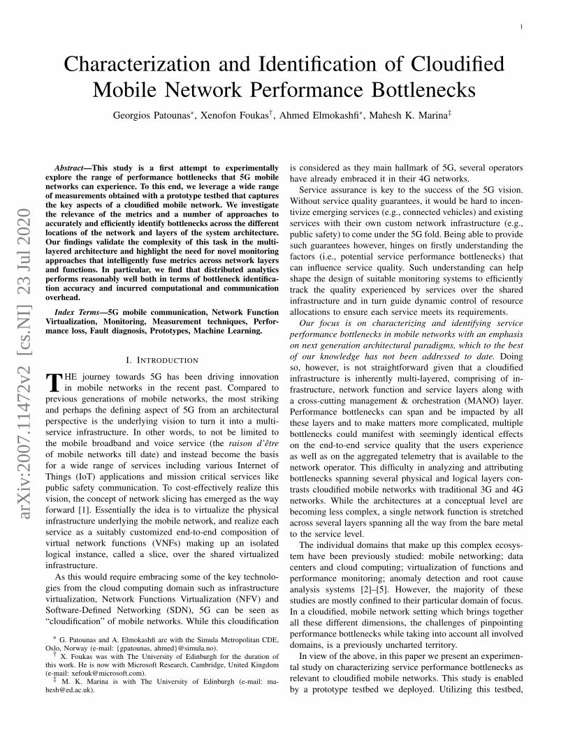
Fig. 1. A generic representation of the 4G network architecture.
components and elements of cloudified mobile networks. Sec-tion III describes our experimental methodology and testbedsetup. Section IV examines different data-driven approachesto discriminating among service performance bottlenecks.Section V approaches the problem from a practical networkmonitoring perspective. Section VI examines the complexitiesof multiple simultaneous bottlenecks. Section VII discussesissues of measurements selection and overhead minimizationas well as the lessons learned. Section VIII discusses relatedwork. Finally, conclusions are provided in Section IX.
II. BACKGROUND
Generally speaking, mobile networks are composed of twomain components: the Core Network (CN) and the RadioAccess Network (RAN). Considering currently deployed 4Gnetworks as an example (see Fig. 1, the CN, referred to asevolved packet core (EPC) in 4G, contains several entitiesincluding: the Packet Data Network Gateway (PGW) whichacts as the gateway between the mobile and external networks;the Serving Gateway (SGW) which manages user equipment(UE) context and acts as its mobility anchor; the MobilityManagement Entity (MME) which performs control actionssuch as SGW selection, UE paging and tagging, etc.; and theHome Subscriber Server (HSS) which manages registration ofusers on the network and functionalities like policy enforce-ment and charging. The CN has traditionally been realizedvia dedicated, high-performance hardware that is distributedin a small number of locations that cover wide areas withmillions of users (e.g., 10-20 per provider in the US). Onthe other hand, the RAN is tasked with providing the wirelessaccess to users and a host of other procedures needed to ensurethat each user can join the network, maintain connectivityover time and use the network services. The RAN consists ofthousands of base stations that carry the necessary wireless,compute and networking equipment in a unit called eNodeB(eNB) in the 4G architecture. As with the CN, the RANand eNBs are also traditionally built on specialized hardwaregeographically distributed to provide the necessary coverageand performance to the users throughout the network (i.e., highdensity is needed in urban areas).
The fact that the network infrastructure consists of special-ized hardware, means that it needs to be statically provisionedand is not easily modifiable. The inherent inflexibility of thisapproach along with the spatio-temporal volatility of usersand their traffic mean that the task of provisioning resourcesefficiently and sufficiently is extremely difficult. In addition,
3
Configuration Life-Cycle
Service Layer
Enterprise 3rd partyVerticalsOperators
Network Function Layer
Infrastructure Layer
Man
agem
ent &
Orch
estra
tion
(MA
NO
)
Control Allocation
Mappin g
EdgeServers
Network
VNFs Network
CoreServers
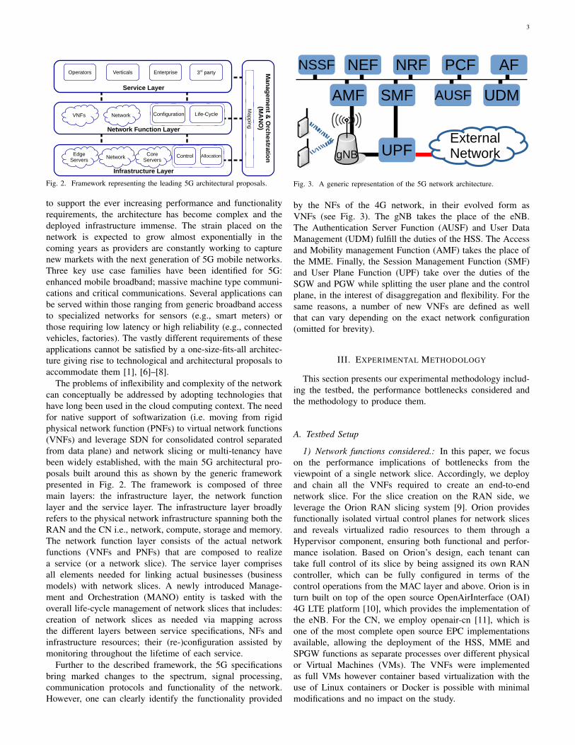
Fig. 2. Framework representing the leading 5G architectural proposals.
to support the ever increasing performance and functionalityrequirements, the architecture has become complex and thedeployed infrastructure immense. The strain placed on thenetwork is expected to grow almost exponentially in thecoming years as providers are constantly working to capturenew markets with the next generation of 5G mobile networks.Three key use case families have been identified for 5G:enhanced mobile broadband; massive machine type communi-cations and critical communications. Several applications canbe served within those ranging from generic broadband accessto specialized networks for sensors (e.g., smart meters) orthose requiring low latency or high reliability (e.g., connectedvehicles, factories). The vastly different requirements of theseapplications cannot be satisfied by a one-size-fits-all architec-ture giving rise to technological and architectural proposals toaccommodate them [1], [6]–[8].
The problems of inflexibility and complexity of the networkcan conceptually be addressed by adopting technologies thathave long been used in the cloud computing context. The needfor native support of softwarization (i.e. moving from rigidphysical network function (PNFs) to virtual network functions(VNFs) and leverage SDN for consolidated control separatedfrom data plane) and network slicing or multi-tenancy havebeen widely established, with the main 5G architectural pro-posals built around this as shown by the generic frameworkpresented in Fig. 2. The framework is composed of threemain layers: the infrastructure layer, the network functionlayer and the service layer. The infrastructure layer broadlyrefers to the physical network infrastructure spanning both theRAN and the CN i.e., network, compute, storage and memory.The network function layer consists of the actual networkfunctions (VNFs and PNFs) that are composed to realizea service (or a network slice). The service layer comprisesall elements needed for linking actual businesses (businessmodels) with network slices. A newly introduced Manage-ment and Orchestration (MANO) entity is tasked with theoverall life-cycle management of network slices that includes:creation of network slices as needed via mapping acrossthe different layers between service specifications, NFs andinfrastructure resources; their (re-)configuration assisted bymonitoring throughout the lifetime of each service.
Further to the described framework, the 5G specificationsbring marked changes to the spectrum, signal processing,communication protocols and functionality of the network.However, one can clearly identify the functionality provided
ExternalNetworkUPF
NEF NRF AFNSSF
AMF SMF
PCF
AUSF
gNB
UDM
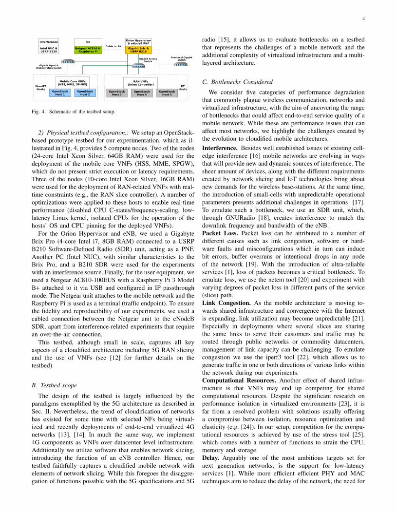
Fig. 3. A generic representation of the 5G network architecture.
by the NFs of the 4G network, in their evolved form asVNFs (see Fig. 3). The gNB takes the place of the eNB.The Authentication Server Function (AUSF) and User DataManagement (UDM) fulfill the duties of the HSS. The Accessand Mobility management Function (AMF) takes the place ofthe MME. Finally, the Session Management Function (SMF)and User Plane Function (UPF) take over the duties of theSGW and PGW while splitting the user plane and the controlplane, in the interest of disaggregation and flexibility. For thesame reasons, a number of new VNFs are defined as wellthat can vary depending on the exact network configuration(omitted for brevity).
III. EXPERIMENTAL METHODOLOGY
This section presents our experimental methodology includ-ing the testbed, the performance bottlenecks considered andthe methodology to produce them.
A. Testbed Setup
1) Network functions considered.: In this paper, we focuson the performance implications of bottlenecks from theviewpoint of a single network slice. Accordingly, we deployand chain all the VNFs required to create an end-to-endnetwork slice. For the slice creation on the RAN side, weleverage the Orion RAN slicing system [9]. Orion providesfunctionally isolated virtual control planes for network slicesand reveals virtualized radio resources to them through aHypervisor component, ensuring both functional and perfor-mance isolation. Based on Orion’s design, each tenant cantake full control of its slice by being assigned its own RANcontroller, which can be fully configured in terms of thecontrol operations from the MAC layer and above. Orion is inturn built on top of the open source OpenAirInterface (OAI)4G LTE platform [10], which provides the implementation ofthe eNB. For the CN, we employ openair-cn [11], which isone of the most complete open source EPC implementationsavailable, allowing the deployment of the HSS, MME andSPGW functions as separate processes over different physicalor Virtual Machines (VMs). The VNFs were implementedas full VMs however container based virtualization with theuse of Linux containers or Docker is possible with minimalmodifications and no impact on the study.
4
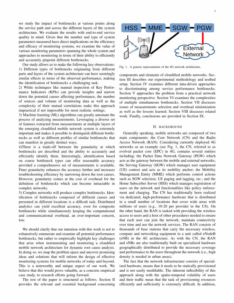
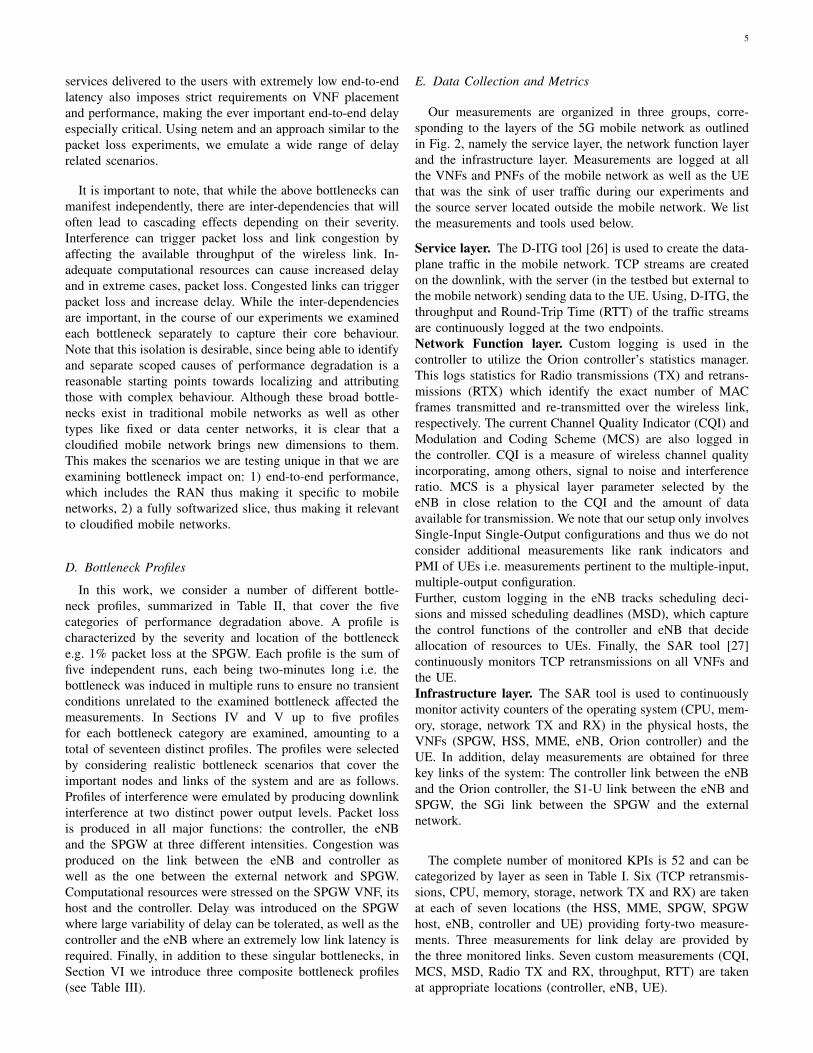
Fig. 4. Schematic of the testbed setup.
2) Physical testbed configuration.: We setup an OpenStack-based prototype testbed for our experimentation, which as il-lustrated in Fig. 4, provides 5 compute nodes. Two of the nodes(24-core Intel Xeon Silver, 64GB RAM) were used for thedeployment of the mobile core VNFs (HSS, MME, SPGW),which do not present strict execution or latency requirements.Three of the nodes (10-core Intel Xeon Silver, 16GB RAM)were used for the deployment of RAN-related VNFs with real-time constraints (e.g., the RAN slice controller). A number ofoptimizations were applied to these hosts to enable real-timeperformance (disabled CPU C-states/frequency-scaling, low-latency Linux kernel, isolated CPUs for the operation of thehosts’ OS and CPU pinning for the deployed VNFs).
For the Orion Hypervisor and eNB, we used a GigabyteBrix Pro (4-core Intel i7, 8GB RAM) connected to a USRPB210 Software-Defined Radio (SDR) unit, acting as a PNF.Another PC (Intel NUC), with similar characteristics to theBrix Pro, and a B210 SDR were used for the experimentswith an interference source. Finally, for the user equipment, weused a Netgear AC810-100EUS with a Raspberry Pi 3 ModelB+ attached to it via USB and configured in IP passthroughmode. The Netgear unit attaches to the mobile network and theRaspberry Pi is used as a terminal (traffic endpoint). To ensurethe fidelity and reproducibility of our experiments, we used acabled connection between the Netgear unit to the eNodeBSDR, apart from interference-related experiments that requirean over-the-air connection.
This testbed, although small in scale, captures all keyaspects of a cloudified architecture including 5G RAN slicingand the use of VNFs (see [12] for further details on thetestbed).
B. Testbed scope
The design of the testbed is largely influenced by theparadigms exemplified by the 5G architecture as described inSec. II. Nevertheless, the trend of cloudification of networkshas existed for some time with selected NFs being virtual-ized and recently deployments of end-to-end virtualized 4Gnetworks [13], [14]. In much the same way, we implement4G components as VNFs over datacenter level infrastructure.Additionally we utilize software that enables network slicing,introducing the function of an eNB controller. Hence, ourtestbed faithfully captures a cloudified mobile network withelements of network slicing. While this foregoes the disaggre-gation of functions possible with the 5G specifications and 5G
radio [15], it allows us to evaluate bottlenecks on a testbedthat represents the challenges of a mobile network and theadditional complexity of virtualized infrastructure and a multi-layered architecture.
C. Bottlenecks Considered
We consider five categories of performance degradationthat commonly plague wireless communication, networks andvirtualized infrastructure, with the aim of uncovering the rangeof bottlenecks that could affect end-to-end service quality of amobile network. While these are performance issues that canaffect most networks, we highlight the challenges created bythe evolution to cloudified mobile architectures.Interference. Besides well established issues of existing cell-edge interference [16] mobile networks are evolving in waysthat will provide new and dynamic sources of interference. Thesheer amount of devices, along with the different requirementscreated by network slicing and IoT technologies bring aboutnew demands for the wireless base-stations. At the same time,the introduction of small-cells with unpredictable operationalparameters presents additional challenges in operations [17].To emulate such a bottleneck, we use an SDR unit, which,through GNURadio [18], creates interference to match thedownlink frequency and bandwidth of the eNB.Packet Loss. Packet loss can be attributed to a number ofdifferent causes such as link congestion, software or hard-ware faults and misconfigurations which in turn can inducebit errors, buffer overruns or intentional drops in any nodeof the network [19]. With the introduction of ultra-reliableservices [1], loss of packets becomes a critical bottleneck. Toemulate loss, we use the netem tool [20] and experiment withvarying degrees of packet loss in different parts of the service(slice) path.Link Congestion. As the mobile architecture is moving to-wards shared infrastructure and convergence with the Internetis expanding, link utilization may become unpredictable [21].Especially in deployments where several slices are sharingthe same links to serve their customers and traffic may berouted through public networks or commodity datacenters,management of link capacity can be challenging. To emulatecongestion we use the iperf3 tool [22], which allows us togenerate traffic in one or both directions of various links withinthe network during our experiments.Computational Resources. Another effect of shared infras-tructure is that VNFs may end up competing for sharedcomputational resources. Despite the significant research onperformance isolation in virtualized environments [23], it isfar from a resolved problem with solutions usually offeringa compromise between isolation, resource optimization andelasticity (e.g. [24]). In our setup, competition for the compu-tational resources is achieved by use of the stress tool [25],which comes with a number of functions to strain the CPU,memory and storage.Delay. Arguably one of the most ambitious targets set fornext generation networks, is the support for low-latencyservices [1]. While more efficient efficient PHY and MACtechniques aim to reduce the delay of the network, the need for
5
services delivered to the users with extremely low end-to-endlatency also imposes strict requirements on VNF placementand performance, making the ever important end-to-end delayespecially critical. Using netem and an approach similar to thepacket loss experiments, we emulate a wide range of delayrelated scenarios.
It is important to note, that while the above bottlenecks canmanifest independently, there are inter-dependencies that willoften lead to cascading effects depending on their severity.Interference can trigger packet loss and link congestion byaffecting the available throughput of the wireless link. In-adequate computational resources can cause increased delayand in extreme cases, packet loss. Congested links can triggerpacket loss and increase delay. While the inter-dependenciesare important, in the course of our experiments we examinedeach bottleneck separately to capture their core behaviour.Note that this isolation is desirable, since being able to identifyand separate scoped causes of performance degradation is areasonable starting points towards localizing and attributingthose with complex behaviour. Although these broad bottle-necks exist in traditional mobile networks as well as othertypes like fixed or data center networks, it is clear that acloudified mobile network brings new dimensions to them.This makes the scenarios we are testing unique in that we areexamining bottleneck impact on: 1) end-to-end performance,which includes the RAN thus making it specific to mobilenetworks, 2) a fully softwarized slice, thus making it relevantto cloudified mobile networks.
D. Bottleneck Profiles
In this work, we consider a number of different bottle-neck profiles, summarized in Table II, that cover the fivecategories of performance degradation above. A profile ischaracterized by the severity and location of the bottlenecke.g. 1% packet loss at the SPGW. Each profile is the sum offive independent runs, each being two-minutes long i.e. thebottleneck was induced in multiple runs to ensure no transientconditions unrelated to the examined bottleneck affected themeasurements. In Sections IV and V up to five profilesfor each bottleneck category are examined, amounting to atotal of seventeen distinct profiles. The profiles were selectedby considering realistic bottleneck scenarios that cover theimportant nodes and links of the system and are as follows.Profiles of interference were emulated by producing downlinkinterference at two distinct power output levels. Packet lossis produced in all major functions: the controller, the eNBand the SPGW at three different intensities. Congestion wasproduced on the link between the eNB and controller aswell as the one between the external network and SPGW.Computational resources were stressed on the SPGW VNF, itshost and the controller. Delay was introduced on the SPGWwhere large variability of delay can be tolerated, as well as thecontroller and the eNB where an extremely low link latency isrequired. Finally, in addition to these singular bottlenecks, inSection VI we introduce three composite bottleneck profiles(see Table III).
E. Data Collection and Metrics
Our measurements are organized in three groups, corre-sponding to the layers of the 5G mobile network as outlinedin Fig. 2, namely the service layer, the network function layerand the infrastructure layer. Measurements are logged at allthe VNFs and PNFs of the mobile network as well as the UEthat was the sink of user traffic during our experiments andthe source server located outside the mobile network. We listthe measurements and tools used below.
Service layer. The D-ITG tool [26] is used to create the data-plane traffic in the mobile network. TCP streams are createdon the downlink, with the server (in the testbed but external tothe mobile network) sending data to the UE. Using, D-ITG, thethroughput and Round-Trip Time (RTT) of the traffic streamsare continuously logged at the two endpoints.Network Function layer. Custom logging is used in thecontroller to utilize the Orion controller’s statistics manager.This logs statistics for Radio transmissions (TX) and retrans-missions (RTX) which identify the exact number of MACframes transmitted and re-transmitted over the wireless link,respectively. The current Channel Quality Indicator (CQI) andModulation and Coding Scheme (MCS) are also logged inthe controller. CQI is a measure of wireless channel qualityincorporating, among others, signal to noise and interferenceratio. MCS is a physical layer parameter selected by theeNB in close relation to the CQI and the amount of dataavailable for transmission. We note that our setup only involvesSingle-Input Single-Output configurations and thus we do notconsider additional measurements like rank indicators andPMI of UEs i.e. measurements pertinent to the multiple-input,multiple-output configuration.Further, custom logging in the eNB tracks scheduling deci-sions and missed scheduling deadlines (MSD), which capturethe control functions of the controller and eNB that decideallocation of resources to UEs. Finally, the SAR tool [27]continuously monitors TCP retransmissions on all VNFs andthe UE.Infrastructure layer. The SAR tool is used to continuouslymonitor activity counters of the operating system (CPU, mem-ory, storage, network TX and RX) in the physical hosts, theVNFs (SPGW, HSS, MME, eNB, Orion controller) and theUE. In addition, delay measurements are obtained for threekey links of the system: The controller link between the eNBand the Orion controller, the S1-U link between the eNB andSPGW, the SGi link between the SPGW and the externalnetwork.
The complete number of monitored KPIs is 52 and can becategorized by layer as seen in Table I. Six (TCP retransmis-sions, CPU, memory, storage, network TX and RX) are takenat each of seven locations (the HSS, MME, SPGW, SPGWhost, eNB, controller and UE) providing forty-two measure-ments. Three measurements for link delay are provided bythe three monitored links. Seven custom measurements (CQI,MCS, MSD, Radio TX and RX, throughput, RTT) are takenat appropriate locations (controller, eNB, UE).
6
IV. ARE DIFFERENT BOTTLENECKS EASILY SEPARABLE?
Today, network operators leverage an array of approachesto identify root causes of performance degradation. Theseinclude the visual inspection of measurements, correlationamong various metrics and more recently machine-learningbased systems that attempt to classify or partition relevantmeasurements [28], [29]. In this section, we explore whethercommon troubleshooting approaches are able to distinguishbetween various bottleneck profiles.
A. Visual Inspection
We begin by visually inspecting each measurement overthe range of our experiments to determine their utility inidentifying the bottlenecks. In the course of visual inspection,a measurement is potentially useful if it provides a markedvariation compared to its baseline value when encountering aspecific bottleneck profile. However, this potential usefulnesscan quickly diminish if the same measurement provides similarvariations for a range of different profiles. Considering theabove, we analyze a subset of the profiles, to exemplify twochallenges of discriminating among bottlenecks: the samebottleneck may occur at different locations in the networkproducing significantly different “signatures” (i.e. the observedeffect to the service quality) and conversely, different bottle-necks manifesting at the same location can produce similar sig-natures hindering the identification of the underlying problem.We should stress here that the observed complexities of bottle-neck identification are by no means an isolated phenomenonand are in fact the norm when considering bottlenecks incomplex networks. We have visually inspected all of theprofiles to find the described challenges to be very common.
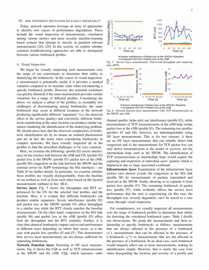
Here, we examine the following: (profile 02) severe interfer-ence on the wireless link between the eNB and UE; (profile 03)packet loss at the SPGW; (profile 07) packet loss at the eNB;(profile 08) congestion on the link between the SPGW and theexternal server (in 3GPP terminology the SGi interface) – seeTable II for further details. In particular, we examine whetherthese profiles are visually distinguishable, from the baselineof our testbed as well as from each other based on the layeredmeasurements outlined in Sec. III-E.Service layer. Fig. 5 shows the throughput and RTT ex-perienced by the UE for the selected four profiles and thebaseline. Here, it is evident that different bottlenecks canproduce similar signatures. Severe interference (profile 02)and packet loss at the SPGW (profile 03) affect throughputin a similar way while the RTT closely matches the baselinemeasurements. On the other hand, congestion on the SGi link(profile 08) and packet loss at the eNB (profile 03) affectboth the throughput and the RTT similarly. Further, it isclear that identical bottlenecks impact end-to-end performancein different ways depending on where they occur, as is thecase with packet loss (profiles 03 and 07). This demonstrateshow service layer measurements are not always sufficient forseparating bottlenecks.Network Function layer. Factoring in NF layer measure-ments, Fig. 6 shows the CQI as well as TCP retransmissionsat the SPGW and the eNB. CQI, which measures radio
● ● ● ● ● ● ● ● ● ● ● ●
●
●
●● ●
●
●
●
●
●
●
●
●● ● ● ●
●● ● ●
● ● ●
● ●● ●
●●
●●
●
● ●●
● ● ● ● ● ● ● ● ● ● ● ●
● ● ● ● ● ● ● ● ● ● ● ●
●
● ●
●
●
●
●
●
●
●
●
●
● ● ● ● ● ● ● ● ● ●● ●
●
●
●
●
●
●
●●
●
● ●
●
● ●● ● ● ● ● ● ●
● ● ●
0123456789
1011
0
200
400
600
800
1000
1200
0 20 40 60 80 100 0 20 40 60 80 100Time (s) Time (s)
Thr
ough
put (
Mbp
s)
RT
T (
ms)
●
●
●
●
●Severe interferenceCongested SGi link
Packet loss at the SPGWPacket loss at the eNB
Baseline
Fig. 5. Service layer measurements: End-to-end throughput and round-triptime (RTT).
● ● ● ● ●● ● ● ● ● ● ●
● ● ● ● ● ● ● ● ● ● ● ●● ● ● ● ● ● ● ● ● ● ● ●● ● ● ● ● ● ● ● ● ● ● ●● ● ● ● ● ● ● ● ● ● ● ●
● ● ● ● ● ● ● ● ● ● ● ●● ● ● ● ● ● ● ● ● ● ● ●● ● ● ● ● ● ● ● ● ● ● ●● ● ● ● ● ● ● ● ● ● ● ●● ● ● ● ● ● ● ● ● ● ● ● ● ● ● ● ● ● ● ● ● ● ● ●● ● ● ● ● ● ● ● ● ● ● ●● ● ● ● ● ● ● ● ● ● ● ●
●
●●
● ●
●
●●
●
●
● ●
● ● ● ● ● ● ● ● ● ● ● ●0
3
6
9
12
15
0
10
20
30
40
50
0
10
20
30
40
50
0 20 40 60 80100 0 20 40 60 80100 0 20 40 60 80100Time (s) Time (s) Time (s)
CQ
I
Ret
rans
./s, S
PG
W
Ret
rans
./s, e
NB
●
●
●
●
●Severe interferenceCongested SGi link
Packet loss at the SPGWPacket loss at the eNB
Baseline
Fig. 6. Network function layer measurements: CQI, TCP retransmissions onthe SPGW and eNB.
channel quality, helps pick out interference (profile 02), whilemeasurements of TCP retransmissions at the eNB help isolatepacket loss at the eNB (profile 03). The remaining two profiles(profiles 07 and 08), however, are indistinguishable usingNF layer measurements. This is for two reasons: i) thereare no NF layer measurements that can reliably detect linkcongestion and ii) the measurements for TCP packet loss canonly detect retransmissions at the sender or receiver, not theintermediate hops such as the SPGW. The identification ofTCP retransmissions in intermediate hops would require thecapturing and inspection of individual users’ packets which isimpractical due to large associated overheads.Infrastructure layer. Examination of the infrastructure layermetrics (not shown) reveals the congestion in the SGi link(profile 08) by measurements of packets transmitted andreceived at the SPGW, finally allowing us to separate it frompacket loss (profile 07). The remaining bottleneck of packetloss (profile 07), while evidently affects the service levelperformance that the user is experiencing (in this case, thethroughput was severely degraded), can’t be traced to a rootcause through visual inspection.
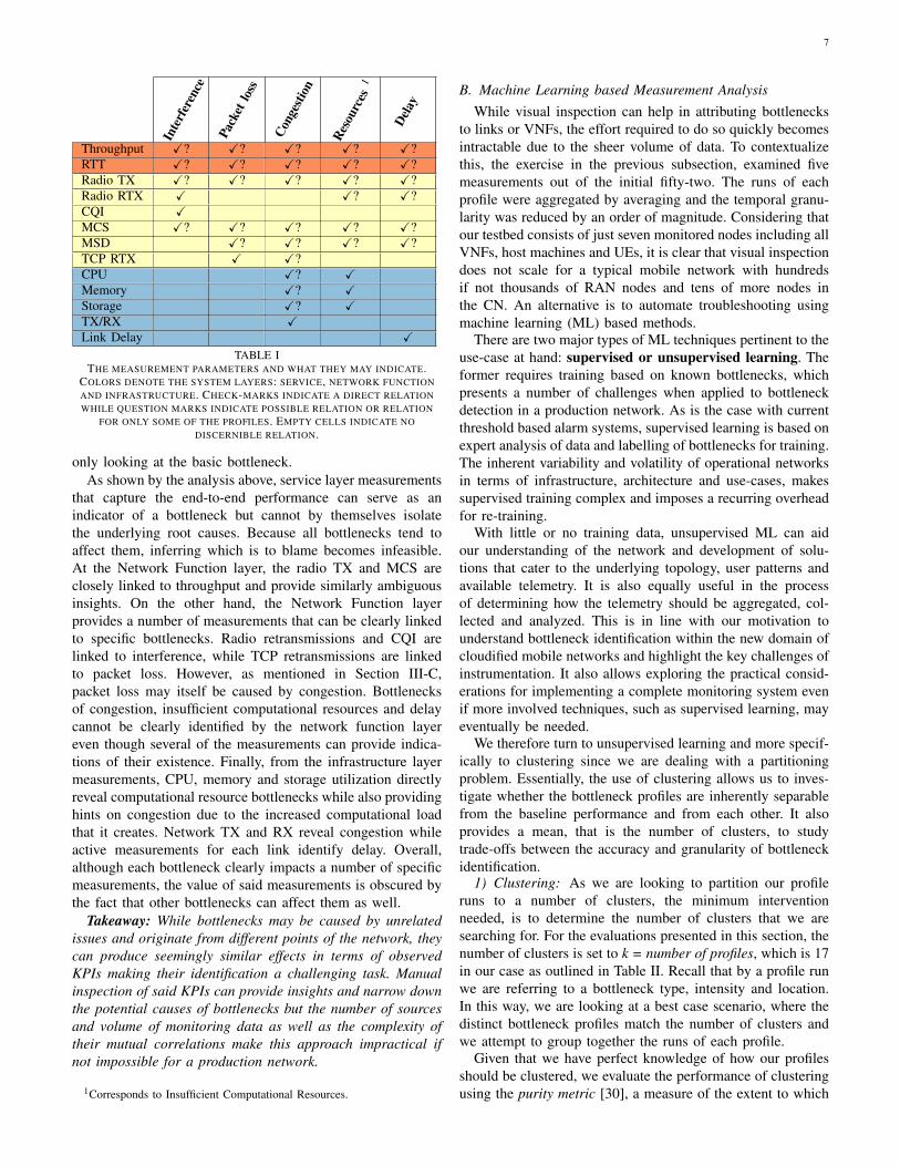
For completeness, we visually inspected all measurementsover the range of bottleneck profiles to determine their utilityfor detecting the considered bottleneck types. Table I distillsour observations. We grade the measurements and their re-lationship to specific bottlenecks as follows: measurementsthat are always affected in the presence of a bottleneck(X), measurements that can be affected in the presence ofa bottleneck (X?) or measurements that are not affected inthe presence of a bottleneck. In an ideal case, each bottleneckwould uniquely affect one or more measurements, making itsidentification simple. However, that is rarely the case evenwhen disregarding the location and severity of a profile and
7
Inte
rfer
ence
Pack
etlo
ss
Cong
estio
n
Reso
urce
s1
Dela
y
Throughput X? X? X? X? X?RTT X? X? X? X? X?Radio TX X? X? X? X? X?Radio RTX X X? X?CQI XMCS X? X? X? X? X?MSD X? X? X? X?TCP RTX X X?CPU X? XMemory X? XStorage X? XTX/RX XLink Delay X
TABLE ITHE MEASUREMENT PARAMETERS AND WHAT THEY MAY INDICATE.
COLORS DENOTE THE SYSTEM LAYERS: SERVICE, NETWORK FUNCTIONAND INFRASTRUCTURE. CHECK-MARKS INDICATE A DIRECT RELATIONWHILE QUESTION MARKS INDICATE POSSIBLE RELATION OR RELATION
FOR ONLY SOME OF THE PROFILES. EMPTY CELLS INDICATE NODISCERNIBLE RELATION.
only looking at the basic bottleneck.As shown by the analysis above, service layer measurements
that capture the end-to-end performance can serve as anindicator of a bottleneck but cannot by themselves isolatethe underlying root causes. Because all bottlenecks tend toaffect them, inferring which is to blame becomes infeasible.At the Network Function layer, the radio TX and MCS areclosely linked to throughput and provide similarly ambiguousinsights. On the other hand, the Network Function layerprovides a number of measurements that can be clearly linkedto specific bottlenecks. Radio retransmissions and CQI arelinked to interference, while TCP retransmissions are linkedto packet loss. However, as mentioned in Section III-C,packet loss may itself be caused by congestion. Bottlenecksof congestion, insufficient computational resources and delaycannot be clearly identified by the network function layereven though several of the measurements can provide indica-tions of their existence. Finally, from the infrastructure layermeasurements, CPU, memory and storage utilization directlyreveal computational resource bottlenecks while also providinghints on congestion due to the increased computational loadthat it creates. Network TX and RX reveal congestion whileactive measurements for each link identify delay. Overall,although each bottleneck clearly impacts a number of specificmeasurements, the value of said measurements is obscured bythe fact that other bottlenecks can affect them as well.
Takeaway: While bottlenecks may be caused by unrelatedissues and originate from different points of the network, theycan produce seemingly similar effects in terms of observedKPIs making their identification a challenging task. Manualinspection of said KPIs can provide insights and narrow downthe potential causes of bottlenecks but the number of sourcesand volume of monitoring data as well as the complexity oftheir mutual correlations make this approach impractical ifnot impossible for a production network.
1Corresponds to Insufficient Computational Resources.
B. Machine Learning based Measurement AnalysisWhile visual inspection can help in attributing bottlenecks
to links or VNFs, the effort required to do so quickly becomesintractable due to the sheer volume of data. To contextualizethis, the exercise in the previous subsection, examined fivemeasurements out of the initial fifty-two. The runs of eachprofile were aggregated by averaging and the temporal granu-larity was reduced by an order of magnitude. Considering thatour testbed consists of just seven monitored nodes including allVNFs, host machines and UEs, it is clear that visual inspectiondoes not scale for a typical mobile network with hundredsif not thousands of RAN nodes and tens of more nodes inthe CN. An alternative is to automate troubleshooting usingmachine learning (ML) based methods.
There are two major types of ML techniques pertinent to theuse-case at hand: supervised or unsupervised learning. Theformer requires training based on known bottlenecks, whichpresents a number of challenges when applied to bottleneckdetection in a production network. As is the case with currentthreshold based alarm systems, supervised learning is based onexpert analysis of data and labelling of bottlenecks for training.The inherent variability and volatility of operational networksin terms of infrastructure, architecture and use-cases, makessupervised training complex and imposes a recurring overheadfor re-training.
With little or no training data, unsupervised ML can aidour understanding of the network and development of solu-tions that cater to the underlying topology, user patterns andavailable telemetry. It is also equally useful in the processof determining how the telemetry should be aggregated, col-lected and analyzed. This is in line with our motivation tounderstand bottleneck identification within the new domain ofcloudified mobile networks and highlight the key challenges ofinstrumentation. It also allows exploring the practical consid-erations for implementing a complete monitoring system evenif more involved techniques, such as supervised learning, mayeventually be needed.
We therefore turn to unsupervised learning and more specif-ically to clustering since we are dealing with a partitioningproblem. Essentially, the use of clustering allows us to inves-tigate whether the bottleneck profiles are inherently separablefrom the baseline performance and from each other. It alsoprovides a mean, that is the number of clusters, to studytrade-offs between the accuracy and granularity of bottleneckidentification.
1) Clustering: As we are looking to partition our profileruns to a number of clusters, the minimum interventionneeded, is to determine the number of clusters that we aresearching for. For the evaluations presented in this section, thenumber of clusters is set to k = number of profiles, which is 17in our case as outlined in Table II. Recall that by a profile runwe are referring to a bottleneck type, intensity and location.In this way, we are looking at a best case scenario, where thedistinct bottleneck profiles match the number of clusters andwe attempt to group together the runs of each profile.
Given that we have perfect knowledge of how our profilesshould be clustered, we evaluate the performance of clusteringusing the purity metric [30], a measure of the extent to which
8
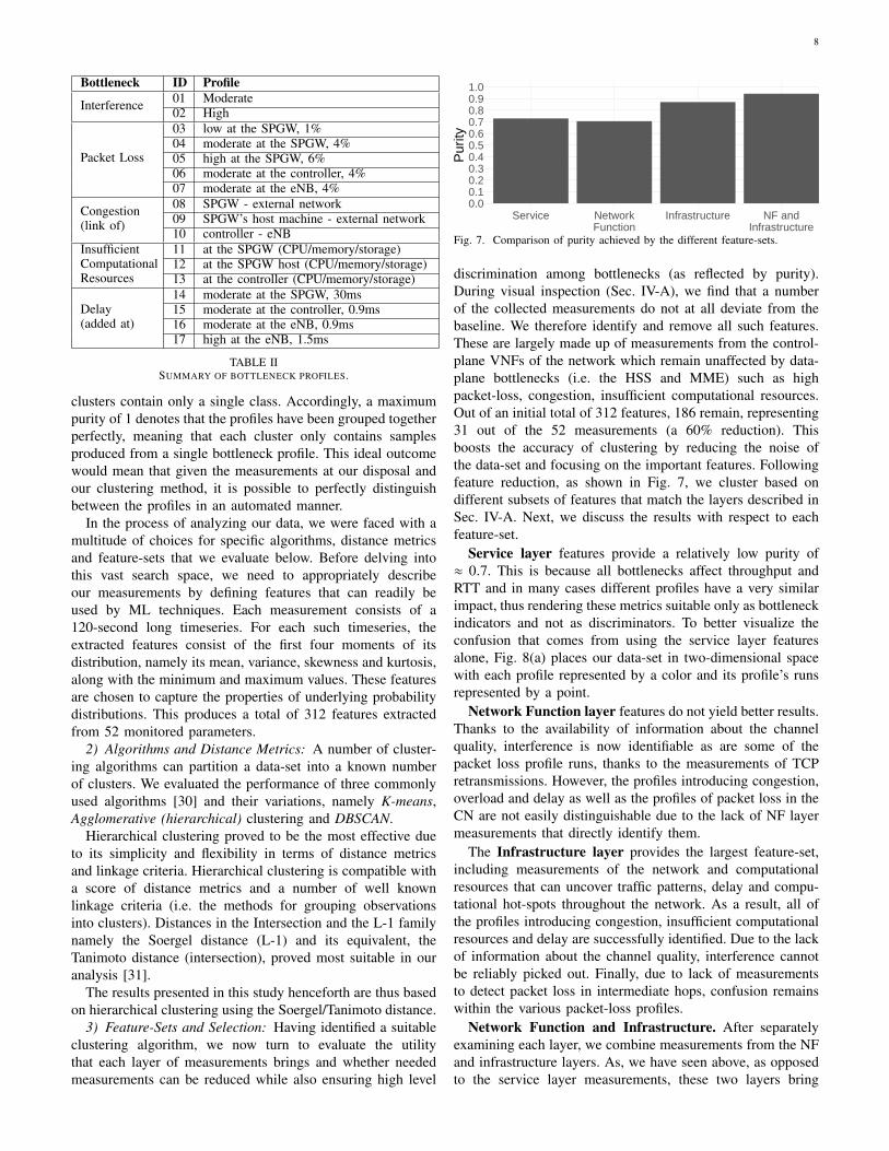
Bottleneck ID Profile
Interference 01 Moderate02 High
Packet Loss
03 low at the SPGW, 1%04 moderate at the SPGW, 4%05 high at the SPGW, 6%06 moderate at the controller, 4%07 moderate at the eNB, 4%
Congestion(link of)
08 SPGW - external network09 SPGW’s host machine - external network10 controller - eNB
InsufficientComputationalResources
11 at the SPGW (CPU/memory/storage)12 at the SPGW host (CPU/memory/storage)13 at the controller (CPU/memory/storage)
Delay(added at)
14 moderate at the SPGW, 30ms15 moderate at the controller, 0.9ms16 moderate at the eNB, 0.9ms17 high at the eNB, 1.5ms
TABLE IISUMMARY OF BOTTLENECK PROFILES.
clusters contain only a single class. Accordingly, a maximumpurity of 1 denotes that the profiles have been grouped togetherperfectly, meaning that each cluster only contains samplesproduced from a single bottleneck profile. This ideal outcomewould mean that given the measurements at our disposal andour clustering method, it is possible to perfectly distinguishbetween the profiles in an automated manner.
In the process of analyzing our data, we were faced with amultitude of choices for specific algorithms, distance metricsand feature-sets that we evaluate below. Before delving intothis vast search space, we need to appropriately describeour measurements by defining features that can readily beused by ML techniques. Each measurement consists of a120-second long timeseries. For each such timeseries, theextracted features consist of the first four moments of itsdistribution, namely its mean, variance, skewness and kurtosis,along with the minimum and maximum values. These featuresare chosen to capture the properties of underlying probabilitydistributions. This produces a total of 312 features extractedfrom 52 monitored parameters.
2) Algorithms and Distance Metrics: A number of cluster-ing algorithms can partition a data-set into a known numberof clusters. We evaluated the performance of three commonlyused algorithms [30] and their variations, namely K-means,Agglomerative (hierarchical) clustering and DBSCAN.
Hierarchical clustering proved to be the most effective dueto its simplicity and flexibility in terms of distance metricsand linkage criteria. Hierarchical clustering is compatible witha score of distance metrics and a number of well knownlinkage criteria (i.e. the methods for grouping observationsinto clusters). Distances in the Intersection and the L-1 familynamely the Soergel distance (L-1) and its equivalent, theTanimoto distance (intersection), proved most suitable in ouranalysis [31].
The results presented in this study henceforth are thus basedon hierarchical clustering using the Soergel/Tanimoto distance.
3) Feature-Sets and Selection: Having identified a suitableclustering algorithm, we now turn to evaluate the utilitythat each layer of measurements brings and whether neededmeasurements can be reduced while also ensuring high level
0.00.10.20.30.40.50.60.70.80.91.0
Service NetworkFunction
Infrastructure NF andInfrastructure
Pur
ity
Fig. 7. Comparison of purity achieved by the different feature-sets.
discrimination among bottlenecks (as reflected by purity).During visual inspection (Sec. IV-A), we find that a numberof the collected measurements do not at all deviate from thebaseline. We therefore identify and remove all such features.These are largely made up of measurements from the control-plane VNFs of the network which remain unaffected by data-plane bottlenecks (i.e. the HSS and MME) such as highpacket-loss, congestion, insufficient computational resources.Out of an initial total of 312 features, 186 remain, representing31 out of the 52 measurements (a 60% reduction). Thisboosts the accuracy of clustering by reducing the noise ofthe data-set and focusing on the important features. Followingfeature reduction, as shown in Fig. 7, we cluster based ondifferent subsets of features that match the layers described inSec. IV-A. Next, we discuss the results with respect to eachfeature-set.
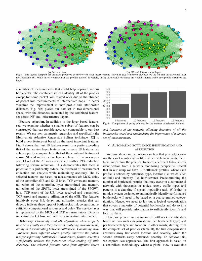
Service layer features provide a relatively low purity of≈ 0.7. This is because all bottlenecks affect throughput andRTT and in many cases different profiles have a very similarimpact, thus rendering these metrics suitable only as bottleneckindicators and not as discriminators. To better visualize theconfusion that comes from using the service layer featuresalone, Fig. 8(a) places our data-set in two-dimensional spacewith each profile represented by a color and its profile’s runsrepresented by a point.
Network Function layer features do not yield better results.Thanks to the availability of information about the channelquality, interference is now identifiable as are some of thepacket loss profile runs, thanks to the measurements of TCPretransmissions. However, the profiles introducing congestion,overload and delay as well as the profiles of packet loss in theCN are not easily distinguishable due to the lack of NF layermeasurements that directly identify them.
The Infrastructure layer provides the largest feature-set,including measurements of the network and computationalresources that can uncover traffic patterns, delay and compu-tational hot-spots throughout the network. As a result, all ofthe profiles introducing congestion, insufficient computationalresources and delay are successfully identified. Due to the lackof information about the channel quality, interference cannotbe reliably picked out. Finally, due to lack of measurementsto detect packet loss in intermediate hops, confusion remainswithin the various packet-loss profiles.
Network Function and Infrastructure. After separatelyexamining each layer, we combine measurements from the NFand infrastructure layers. As, we have seen above, as opposedto the service layer measurements, these two layers bring
9
●●●●●●
●●
●●
●●●●●●
●●
●●
●●●●●●
●●●●
●● ●●●●●●●●
●●●●
●●
●●
●●
●● ●●●●
●●●●
●●
●●
●●
●●
●●●●●●
●●●●●●
●●
●●
●●
●●●●
●●
●● ●●
●●
●●
●●
●●
●●
●● ●●
●●
●●●●
●●
●●●●
●●
●●●●
●●
●●
●●
●●
●●●●
●●●●●●
●●
●●
●●●●
●●●●
●●
●●
●●
●●
●●
●●
1_5_11_5_2
1_5_3
1_5_4
1_5_5
1_6_11_6_2
1_6_3
1_6_4
1_6_5
2_1_1
2_1_2
2_1_3
2_1_4
2_1_5
2_2_12_2_2
2_2_3
2_2_42_2_5
2_3_12_3_2
2_3_3
2_3_4
2_3_5
2_5_1
2_5_2
2_5_3
2_5_4
2_5_5
2_8_1
2_8_2
2_8_3
2_8_4
2_8_5
3_11_1
3_11_2
3_11_33_11_4
3_11_5
3_14_1
3_14_2
3_14_3
3_14_4
3_14_5
3_21_1
3_21_2 3_21_3
3_21_4
3_21_5
4_13_1
4_13_2
4_13_3
4_13_4 4_13_5
4_16_1
4_16_3
4_16_4
4_16_5
4_16_6
4_20_1
4_20_2
4_20_3
4_20_4
4_20_5
6_1_1
6_1_2
6_1_3
6_1_4
6_1_5
6_10_1
6_10_2
6_10_3
6_10_4
6_10_5
6_11_1
6_11_2
6_11_3
6_11_4
6_11_5
6_9_1
6_9_2
6_9_3
6_9_4
6_9_5
(a) Service layer
●●
●●
●●
●●
●● ●●
●●
●●
●●
●●
●●
●●
●●
●●
●●
●●
●●●●
●●
●●
●●●●
●●●●
●●
●●●●
●●
●●
●●
●●
●●
●●
●●
●●
●● ●●
●●
●●
●●
●●●●
●●
●●●●
●●
●●
●●
●●●●
●●
●●
●●
●● ●●
●●
●●
●●
●●
●●
●●●●
●●
●●
●●
●●
●●●●
●●
●●
●● ●●●●●● ●●
●● ●●
●●
●●●●
●● ●●●●
●●
●●
1_5_1
1_5_2
1_5_3
1_5_4
1_5_5 1_6_1
1_6_2
1_6_3
1_6_4
1_6_5
2_1_1
2_1_2
2_1_3
2_1_4
2_1_5
2_2_1
2_2_2
2_2_3
2_2_4
2_2_5
2_3_1
2_3_2
2_3_3
2_3_4
2_3_5
2_5_1
2_5_2
2_5_3
2_5_4
2_5_5
2_8_1
2_8_2
2_8_3
2_8_4
2_8_5
3_11_13_11_2
3_11_3
3_11_4
3_11_5
3_14_1
3_14_2
3_14_3
3_14_4
3_14_5
3_21_1
3_21_2
3_21_3
3_21_4
3_21_5
4_13_1
4_13_2
4_13_3
4_13_4 4_13_5
4_16_1
4_16_3
4_16_4
4_16_5
4_16_6
4_20_1
4_20_2
4_20_3
4_20_4
4_20_5
6_1_1
6_1_2
6_1_3
6_1_4
6_1_5
6_10_1
6_10_26_10_3
6_10_46_10_5
6_11_1
6_11_2
6_11_3
6_11_4
6_11_5
6_9_1 6_9_2
6_9_3
6_9_4
6_9_5
(b) NF and Infrastructure layersFig. 8. The figures compare the distances produced by the service layer measurements (shown in (a)) with those produced by the NF and infrastructure layermeasurements (b). While in (a) confusion of the profiles (colors) is visible, in (b) intra-profile distances are visibly shorter while inter-profile distances arelarger.
a number of measurements that could help separate variousbottlenecks. The combined set can identify all of the profilesexcept for some packet loss related ones due to the absenceof packet loss measurements at intermediate hops. To bettervisualize the improvement in intra-profile and inter-profiledistances, Fig. 8(b) places our data-set in two-dimensionalspace, with the distances calculated by the combined feature-set across NF and infrastructure layers.
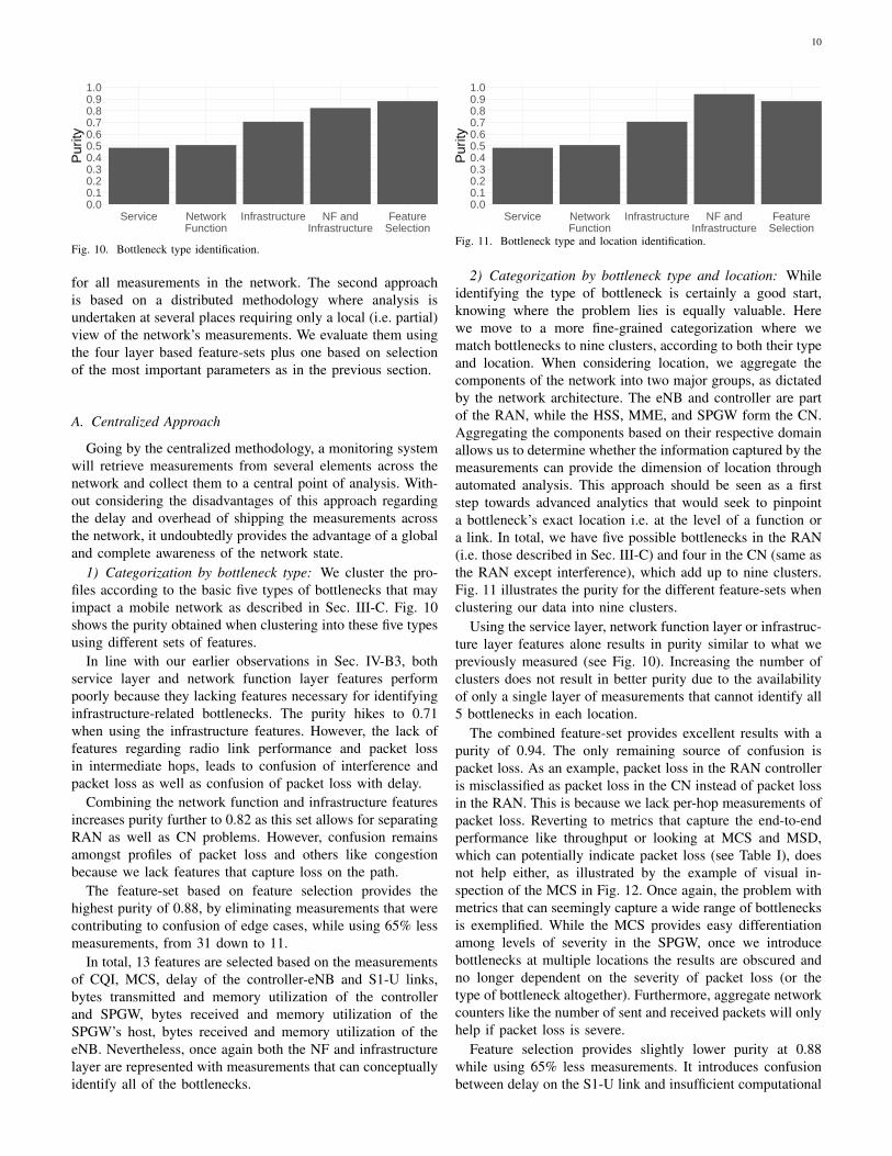
Feature selection. In addition to the layer based feature-sets we examine whether a smaller subset of features can beconstructed that can provide accuracy comparable to our bestresults. We use non-parametric regression and specifically theMultivariate Adaptive Regression Splines technique [32] tobuild a new feature-set based on the most important features.Fig. 9 shows that just 10 features result in a purity exceedingthat of the service layer features and a mere 19 features canachieve purity comparable to that of the combined feature-setacross NF and infrastructure layers. These 19 features repre-sent 13 out of the 31 measurements, a further 59% reductionfollowing feature reduction. This demonstrates that there ispotential to significantly reduce the overhead of measurementcollection and analysis while maintaining accuracy. The 19selected features are based on measurements of: MCS, delayof the controller-eNB and S1-U links, TCP errors and memoryutilization of the controller, bytes transmitted and memoryutilization of the SPGW, bytes transmitted of the SPGW’shost, TCP errors of the UE, bytes received and transmitted,TCP errors and memory utilization of the eNB. The featuresintuitively cover link delay, and utilization metrics that candirectly indicate three types of bottlenecks: link congestion, in-sufficient computational resources and delay. The service layeris represented by the MCS and TCP retransmissions. Directlyindicating packet loss and indirectly indicating interference.
Takeaway: Commonly used ML algorithms when properlytuned can greatly ease the process of analyzing measurements,aiding in discriminating between bottlenecks. Combining mea-surements from different layers greatly improves the poten-tial for separating bottlenecks. Furthermore, feature selectionsignificantly reduces the feature-set while trading off littleaccuracy. The selected features come from different layers
0.00.10.20.30.40.50.60.70.80.91.0
5 features 10 features 15 features 19 features
Pur
ity
Fig. 9. Comparison of purity achieved by the number of selected features.
and locations of the network, allowing detection of all thebottlenecks tested and emphasizing the importance of a diverseset of measurements.
V. AUTOMATING BOTTLENECK IDENTIFICATION ANDATTRIBUTION
We have shown in the previous section that precisely know-ing the exact number of profiles, we are able to separate them.Next, we explore the practical trade-offs pertinent to bottleneckidentification from a network monitoring perspective. Recallthat in our setup we have 17 bottleneck profiles, where eachprofile is defined by bottleneck type, location (i.e. which VNFor link) and intensity (i.e. how severe). Predetermining thenumber of bottleneck profiles that may occur in a commercialnetwork with thousands of nodes, users, traffic types andpatterns is a daunting if not an impossible task. With that inmind, a system designed to automatically identify performancebottlenecks will need to be based on a coarse-grained catego-rization. Hence, we need to lay out a logical categorizationthat covers a majority of potential bottlenecks and do so in away that will provide information to sufficiently identify andlocalize them.
Here, we present an evaluation of bottleneck identificationbased on two such categorizations: per bottleneck type; andper bottleneck type and location. In other words, starting fromthe complete set of profiles (Table II), the first categorizationabstracts away bottleneck location and severity, while thesecond abstracts away bottleneck severity. To achieve this,we explore two approaches. The first approach is based ona centralized methodology where a global view is available
10
0.00.10.20.30.40.50.60.70.80.91.0
Service NetworkFunction
Infrastructure NF andInfrastructure
FeatureSelection
Pur
ity
Fig. 10. Bottleneck type identification.
for all measurements in the network. The second approachis based on a distributed methodology where analysis isundertaken at several places requiring only a local (i.e. partial)view of the network’s measurements. We evaluate them usingthe four layer based feature-sets plus one based on selectionof the most important parameters as in the previous section.
A. Centralized Approach
Going by the centralized methodology, a monitoring systemwill retrieve measurements from several elements across thenetwork and collect them to a central point of analysis. With-out considering the disadvantages of this approach regardingthe delay and overhead of shipping the measurements acrossthe network, it undoubtedly provides the advantage of a globaland complete awareness of the network state.
1) Categorization by bottleneck type: We cluster the pro-files according to the basic five types of bottlenecks that mayimpact a mobile network as described in Sec. III-C. Fig. 10shows the purity obtained when clustering into these five typesusing different sets of features.
In line with our earlier observations in Sec. IV-B3, bothservice layer and network function layer features performpoorly because they lacking features necessary for identifyinginfrastructure-related bottlenecks. The purity hikes to 0.71when using the infrastructure features. However, the lack offeatures regarding radio link performance and packet lossin intermediate hops, leads to confusion of interference andpacket loss as well as confusion of packet loss with delay.
Combining the network function and infrastructure featuresincreases purity further to 0.82 as this set allows for separatingRAN as well as CN problems. However, confusion remainsamongst profiles of packet loss and others like congestionbecause we lack features that capture loss on the path.
The feature-set based on feature selection provides thehighest purity of 0.88, by eliminating measurements that werecontributing to confusion of edge cases, while using 65% lessmeasurements, from 31 down to 11.
In total, 13 features are selected based on the measurementsof CQI, MCS, delay of the controller-eNB and S1-U links,bytes transmitted and memory utilization of the controllerand SPGW, bytes received and memory utilization of theSPGW’s host, bytes received and memory utilization of theeNB. Nevertheless, once again both the NF and infrastructurelayer are represented with measurements that can conceptuallyidentify all of the bottlenecks.
0.00.10.20.30.40.50.60.70.80.91.0
Service NetworkFunction
Infrastructure NF andInfrastructure
FeatureSelection
Pur
ity
Fig. 11. Bottleneck type and location identification.
2) Categorization by bottleneck type and location: Whileidentifying the type of bottleneck is certainly a good start,knowing where the problem lies is equally valuable. Herewe move to a more fine-grained categorization where wematch bottlenecks to nine clusters, according to both their typeand location. When considering location, we aggregate thecomponents of the network into two major groups, as dictatedby the network architecture. The eNB and controller are partof the RAN, while the HSS, MME, and SPGW form the CN.Aggregating the components based on their respective domainallows us to determine whether the information captured by themeasurements can provide the dimension of location throughautomated analysis. This approach should be seen as a firststep towards advanced analytics that would seek to pinpointa bottleneck’s exact location i.e. at the level of a function ora link. In total, we have five possible bottlenecks in the RAN(i.e. those described in Sec. III-C) and four in the CN (same asthe RAN except interference), which add up to nine clusters.Fig. 11 illustrates the purity for the different feature-sets whenclustering our data into nine clusters.
Using the service layer, network function layer or infrastruc-ture layer features alone results in purity similar to what wepreviously measured (see Fig. 10). Increasing the number ofclusters does not result in better purity due to the availabilityof only a single layer of measurements that cannot identify all5 bottlenecks in each location.
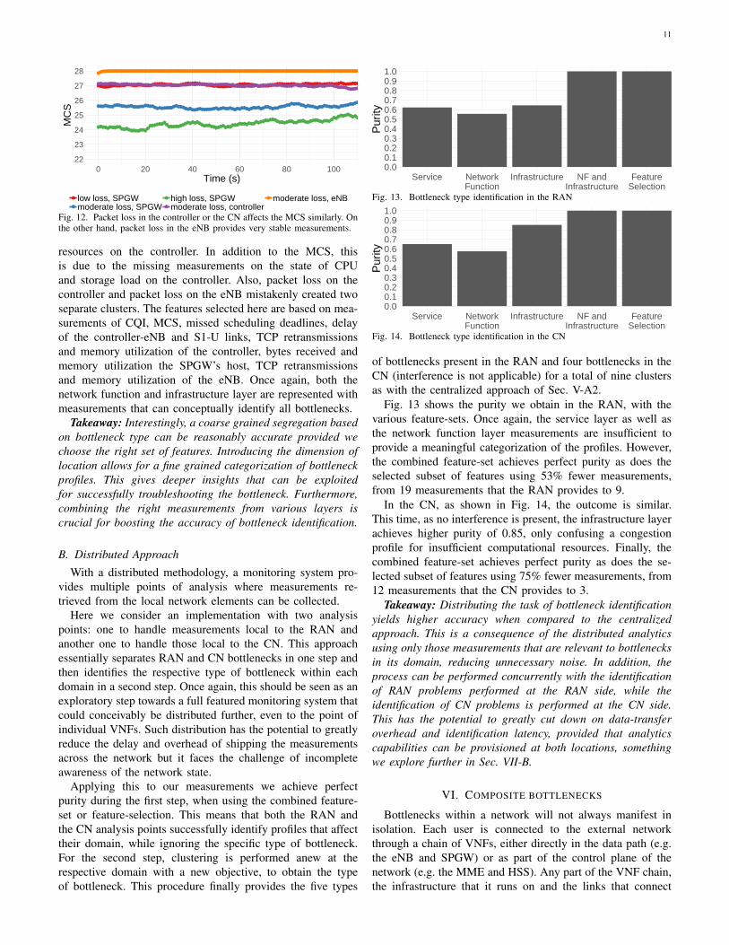
The combined feature-set provides excellent results with apurity of 0.94. The only remaining source of confusion ispacket loss. As an example, packet loss in the RAN controlleris misclassified as packet loss in the CN instead of packet lossin the RAN. This is because we lack per-hop measurements ofpacket loss. Reverting to metrics that capture the end-to-endperformance like throughput or looking at MCS and MSD,which can potentially indicate packet loss (see Table I), doesnot help either, as illustrated by the example of visual in-spection of the MCS in Fig. 12. Once again, the problem withmetrics that can seemingly capture a wide range of bottlenecksis exemplified. While the MCS provides easy differentiationamong levels of severity in the SPGW, once we introducebottlenecks at multiple locations the results are obscured andno longer dependent on the severity of packet loss (or thetype of bottleneck altogether). Furthermore, aggregate networkcounters like the number of sent and received packets will onlyhelp if packet loss is severe.
Feature selection provides slightly lower purity at 0.88while using 65% less measurements. It introduces confusionbetween delay on the S1-U link and insufficient computational
11
●●●●●●●●●●●●●●●●●●●●●●●●●●●●●●●●●●●●●●●●●●●●●●●●●●●●●●●●●●●●●●●●●●●●●●●●●●●●●●●●●●●●●●●●●●●●●●●●●●●●●●●●●●●●●●●
●●●●●●●●●●●●●●●●●●●●●●●●●●●●●●●●●●●●●●●●●●●●●●●●●●●●●●●●●●●●●●●●●●●●●●●●●●●●●●●●●●●●●●●●●●●●●●●●●●●●●●●●●●●●●●●
●●●●●●●●●●●●●●●●●●●●●
●●●●●●●●
●●●●●●●●●●●●●●●●●●●●●●●●●●●●
●●●●●●●●●●●●●●●●●●●●●●●●●●●●●●●●●●●●●●●●●●●
●●●●●●●●●●●
●●●●●●●●●●●●●●●●●●●●●●●●●●●●●●●●●●●●●●●●●●●●●●●●●●●●●●●●●●●●●●●●●●●●●●●●●●●●●●●●●●●●●●●●●●●●●●●●●●●●●●●●●●●●●●●
●●●●●●●●●●●●●●●●●●●●●●●●●●●●●●●●●●●●●●●●●●●●●●●●●●●●●●●●●●●●●●●●●●●●●●●●●●●●●●●●●●●●●●●●●●●●●●●●●●●●●●●●●●●●●●●
22
23
24
25
26
27
28
0 20 40 60 80 100Time (s)
MC
S
●
●
●
●
●low loss, SPGWmoderate loss, SPGW
high loss, SPGWmoderate loss, controller
moderate loss, eNB
Fig. 12. Packet loss in the controller or the CN affects the MCS similarly. Onthe other hand, packet loss in the eNB provides very stable measurements.
resources on the controller. In addition to the MCS, thisis due to the missing measurements on the state of CPUand storage load on the controller. Also, packet loss on thecontroller and packet loss on the eNB mistakenly created twoseparate clusters. The features selected here are based on mea-surements of CQI, MCS, missed scheduling deadlines, delayof the controller-eNB and S1-U links, TCP retransmissionsand memory utilization of the controller, bytes received andmemory utilization the SPGW’s host, TCP retransmissionsand memory utilization of the eNB. Once again, both thenetwork function and infrastructure layer are represented withmeasurements that can conceptually identify all bottlenecks.
Takeaway: Interestingly, a coarse grained segregation basedon bottleneck type can be reasonably accurate provided wechoose the right set of features. Introducing the dimension oflocation allows for a fine grained categorization of bottleneckprofiles. This gives deeper insights that can be exploitedfor successfully troubleshooting the bottleneck. Furthermore,combining the right measurements from various layers iscrucial for boosting the accuracy of bottleneck identification.
B. Distributed Approach
With a distributed methodology, a monitoring system pro-vides multiple points of analysis where measurements re-trieved from the local network elements can be collected.
Here we consider an implementation with two analysispoints: one to handle measurements local to the RAN andanother one to handle those local to the CN. This approachessentially separates RAN and CN bottlenecks in one step andthen identifies the respective type of bottleneck within eachdomain in a second step. Once again, this should be seen as anexploratory step towards a full featured monitoring system thatcould conceivably be distributed further, even to the point ofindividual VNFs. Such distribution has the potential to greatlyreduce the delay and overhead of shipping the measurementsacross the network but it faces the challenge of incompleteawareness of the network state.
Applying this to our measurements we achieve perfectpurity during the first step, when using the combined feature-set or feature-selection. This means that both the RAN andthe CN analysis points successfully identify profiles that affecttheir domain, while ignoring the specific type of bottleneck.For the second step, clustering is performed anew at therespective domain with a new objective, to obtain the typeof bottleneck. This procedure finally provides the five types
0.00.10.20.30.40.50.60.70.80.91.0
Service NetworkFunction
Infrastructure NF andInfrastructure
FeatureSelection
Pur
ity
Fig. 13. Bottleneck type identification in the RAN
0.00.10.20.30.40.50.60.70.80.91.0
Service NetworkFunction
Infrastructure NF andInfrastructure
FeatureSelection
Pur
ity
Fig. 14. Bottleneck type identification in the CN
of bottlenecks present in the RAN and four bottlenecks in theCN (interference is not applicable) for a total of nine clustersas with the centralized approach of Sec. V-A2.
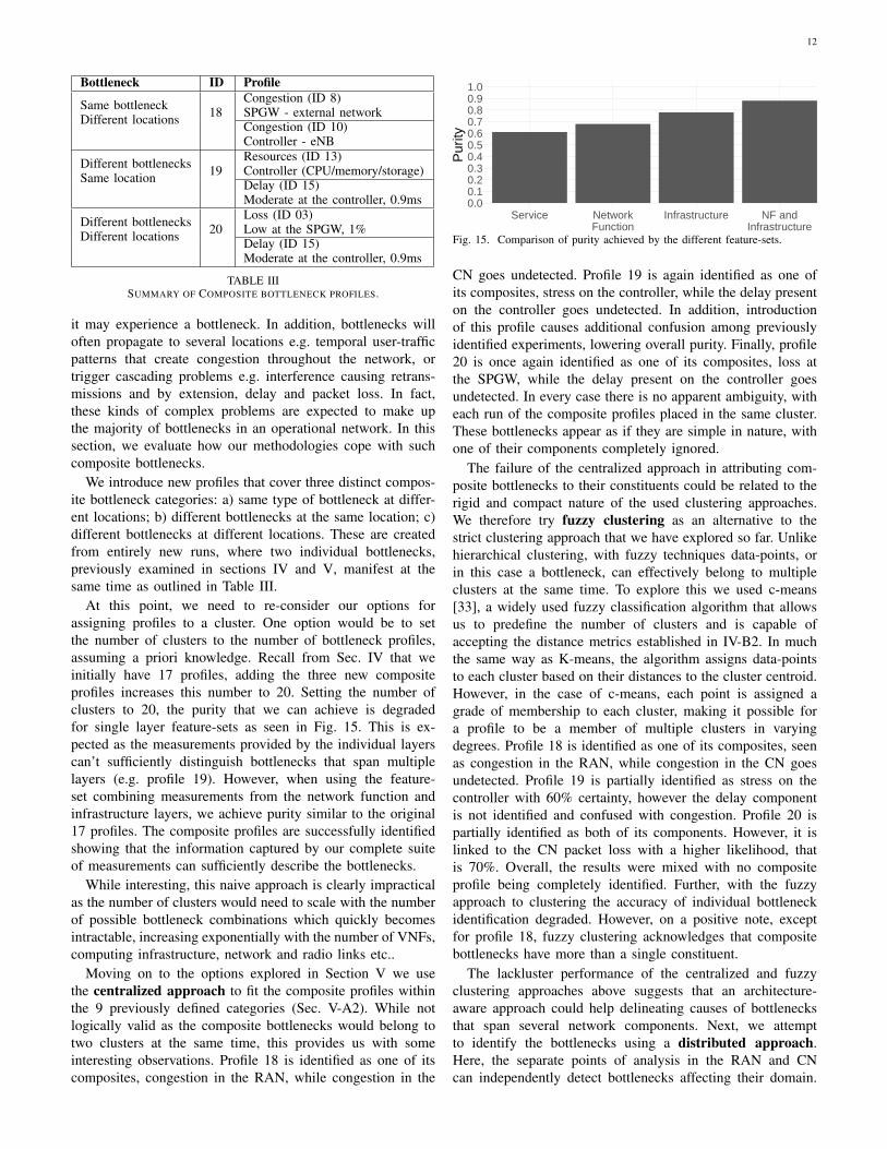
Fig. 13 shows the purity we obtain in the RAN, with thevarious feature-sets. Once again, the service layer as well asthe network function layer measurements are insufficient toprovide a meaningful categorization of the profiles. However,the combined feature-set achieves perfect purity as does theselected subset of features using 53% fewer measurements,from 19 measurements that the RAN provides to 9.
In the CN, as shown in Fig. 14, the outcome is similar.This time, as no interference is present, the infrastructure layerachieves higher purity of 0.85, only confusing a congestionprofile for insufficient computational resources. Finally, thecombined feature-set achieves perfect purity as does the se-lected subset of features using 75% fewer measurements, from12 measurements that the CN provides to 3.
Takeaway: Distributing the task of bottleneck identificationyields higher accuracy when compared to the centralizedapproach. This is a consequence of the distributed analyticsusing only those measurements that are relevant to bottlenecksin its domain, reducing unnecessary noise. In addition, theprocess can be performed concurrently with the identificationof RAN problems performed at the RAN side, while theidentification of CN problems is performed at the CN side.This has the potential to greatly cut down on data-transferoverhead and identification latency, provided that analyticscapabilities can be provisioned at both locations, somethingwe explore further in Sec. VII-B.
VI. COMPOSITE BOTTLENECKS
Bottlenecks within a network will not always manifest inisolation. Each user is connected to the external networkthrough a chain of VNFs, either directly in the data path (e.g.the eNB and SPGW) or as part of the control plane of thenetwork (e.g. the MME and HSS). Any part of the VNF chain,the infrastructure that it runs on and the links that connect
12
Bottleneck ID Profile
Same bottleneckDifferent locations 18
Congestion (ID 8)SPGW - external networkCongestion (ID 10)Controller - eNB
Different bottlenecksSame location 19
Resources (ID 13)Controller (CPU/memory/storage)Delay (ID 15)Moderate at the controller, 0.9ms
Different bottlenecksDifferent locations 20
Loss (ID 03)Low at the SPGW, 1%Delay (ID 15)Moderate at the controller, 0.9ms
TABLE IIISUMMARY OF COMPOSITE BOTTLENECK PROFILES.
it may experience a bottleneck. In addition, bottlenecks willoften propagate to several locations e.g. temporal user-trafficpatterns that create congestion throughout the network, ortrigger cascading problems e.g. interference causing retrans-missions and by extension, delay and packet loss. In fact,these kinds of complex problems are expected to make upthe majority of bottlenecks in an operational network. In thissection, we evaluate how our methodologies cope with suchcomposite bottlenecks.
We introduce new profiles that cover three distinct compos-ite bottleneck categories: a) same type of bottleneck at differ-ent locations; b) different bottlenecks at the same location; c)different bottlenecks at different locations. These are createdfrom entirely new runs, where two individual bottlenecks,previously examined in sections IV and V, manifest at thesame time as outlined in Table III.
At this point, we need to re-consider our options forassigning profiles to a cluster. One option would be to setthe number of clusters to the number of bottleneck profiles,assuming a priori knowledge. Recall from Sec. IV that weinitially have 17 profiles, adding the three new compositeprofiles increases this number to 20. Setting the number ofclusters to 20, the purity that we can achieve is degradedfor single layer feature-sets as seen in Fig. 15. This is ex-pected as the measurements provided by the individual layerscan’t sufficiently distinguish bottlenecks that span multiplelayers (e.g. profile 19). However, when using the feature-set combining measurements from the network function andinfrastructure layers, we achieve purity similar to the original17 profiles. The composite profiles are successfully identifiedshowing that the information captured by our complete suiteof measurements can sufficiently describe the bottlenecks.
While interesting, this naive approach is clearly impracticalas the number of clusters would need to scale with the numberof possible bottleneck combinations which quickly becomesintractable, increasing exponentially with the number of VNFs,computing infrastructure, network and radio links etc..
Moving on to the options explored in Section V we usethe centralized approach to fit the composite profiles withinthe 9 previously defined categories (Sec. V-A2). While notlogically valid as the composite bottlenecks would belong totwo clusters at the same time, this provides us with someinteresting observations. Profile 18 is identified as one of itscomposites, congestion in the RAN, while congestion in the
0.00.10.20.30.40.50.60.70.80.91.0
Service NetworkFunction
Infrastructure NF andInfrastructure
Pur
ity
Fig. 15. Comparison of purity achieved by the different feature-sets.
CN goes undetected. Profile 19 is again identified as one ofits composites, stress on the controller, while the delay presenton the controller goes undetected. In addition, introductionof this profile causes additional confusion among previouslyidentified experiments, lowering overall purity. Finally, profile20 is once again identified as one of its composites, loss atthe SPGW, while the delay present on the controller goesundetected. In every case there is no apparent ambiguity, witheach run of the composite profiles placed in the same cluster.These bottlenecks appear as if they are simple in nature, withone of their components completely ignored.
The failure of the centralized approach in attributing com-posite bottlenecks to their constituents could be related to therigid and compact nature of the used clustering approaches.We therefore try fuzzy clustering as an alternative to thestrict clustering approach that we have explored so far. Unlikehierarchical clustering, with fuzzy techniques data-points, orin this case a bottleneck, can effectively belong to multipleclusters at the same time. To explore this we used c-means[33], a widely used fuzzy classification algorithm that allowsus to predefine the number of clusters and is capable ofaccepting the distance metrics established in IV-B2. In muchthe same way as K-means, the algorithm assigns data-pointsto each cluster based on their distances to the cluster centroid.However, in the case of c-means, each point is assigned agrade of membership to each cluster, making it possible fora profile to be a member of multiple clusters in varyingdegrees. Profile 18 is identified as one of its composites, seenas congestion in the RAN, while congestion in the CN goesundetected. Profile 19 is partially identified as stress on thecontroller with 60% certainty, however the delay componentis not identified and confused with congestion. Profile 20 ispartially identified as both of its components. However, it islinked to the CN packet loss with a higher likelihood, thatis 70%. Overall, the results were mixed with no compositeprofile being completely identified. Further, with the fuzzyapproach to clustering the accuracy of individual bottleneckidentification degraded. However, on a positive note, exceptfor profile 18, fuzzy clustering acknowledges that compositebottlenecks have more than a single constituent.
The lackluster performance of the centralized and fuzzyclustering approaches above suggests that an architecture-aware approach could help delineating causes of bottlenecksthat span several network components. Next, we attemptto identify the bottlenecks using a distributed approach.Here, the separate points of analysis in the RAN and CNcan independently detect bottlenecks affecting their domain.
13
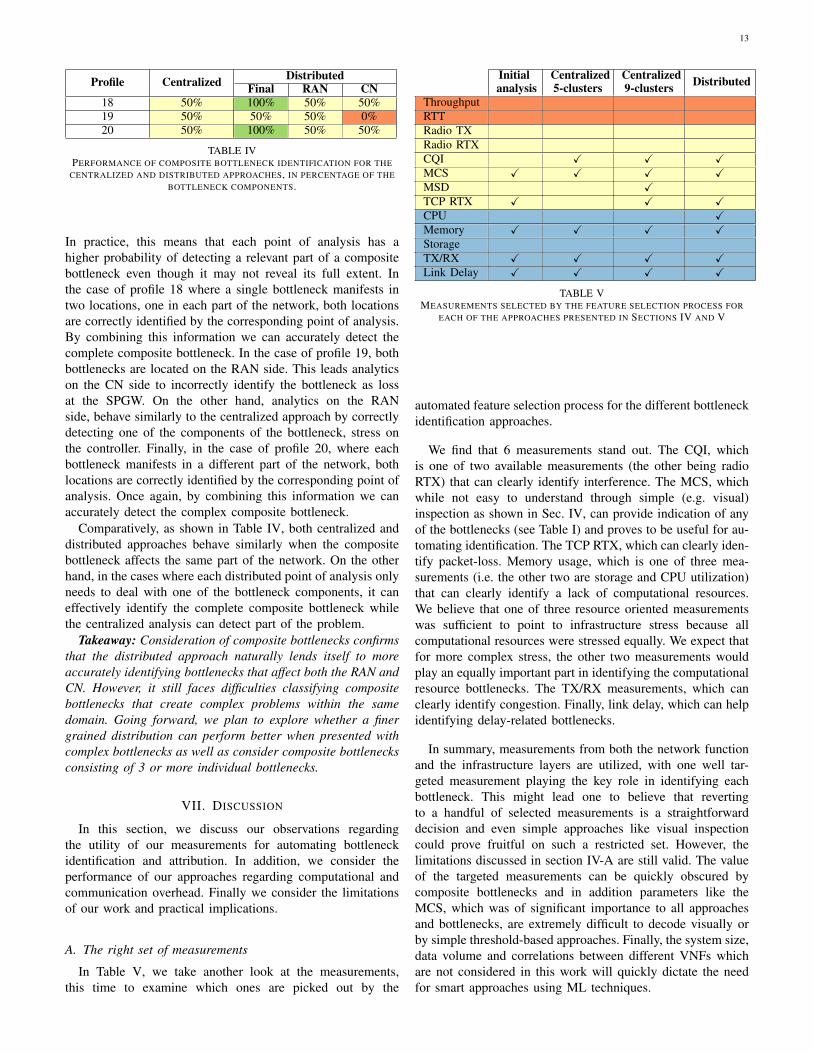
Profile Centralized DistributedFinal RAN CN
18 50% 100% 50% 50%19 50% 50% 50% 0%20 50% 100% 50% 50%
TABLE IVPERFORMANCE OF COMPOSITE BOTTLENECK IDENTIFICATION FOR THE
CENTRALIZED AND DISTRIBUTED APPROACHES, IN PERCENTAGE OF THEBOTTLENECK COMPONENTS.
In practice, this means that each point of analysis has ahigher probability of detecting a relevant part of a compositebottleneck even though it may not reveal its full extent. Inthe case of profile 18 where a single bottleneck manifests intwo locations, one in each part of the network, both locationsare correctly identified by the corresponding point of analysis.By combining this information we can accurately detect thecomplete composite bottleneck. In the case of profile 19, bothbottlenecks are located on the RAN side. This leads analyticson the CN side to incorrectly identify the bottleneck as lossat the SPGW. On the other hand, analytics on the RANside, behave similarly to the centralized approach by correctlydetecting one of the components of the bottleneck, stress onthe controller. Finally, in the case of profile 20, where eachbottleneck manifests in a different part of the network, bothlocations are correctly identified by the corresponding point ofanalysis. Once again, by combining this information we canaccurately detect the complex composite bottleneck.
Comparatively, as shown in Table IV, both centralized anddistributed approaches behave similarly when the compositebottleneck affects the same part of the network. On the otherhand, in the cases where each distributed point of analysis onlyneeds to deal with one of the bottleneck components, it caneffectively identify the complete composite bottleneck whilethe centralized analysis can detect part of the problem.
Takeaway: Consideration of composite bottlenecks confirmsthat the distributed approach naturally lends itself to moreaccurately identifying bottlenecks that affect both the RAN andCN. However, it still faces difficulties classifying compositebottlenecks that create complex problems within the samedomain. Going forward, we plan to explore whether a finergrained distribution can perform better when presented withcomplex bottlenecks as well as consider composite bottlenecksconsisting of 3 or more individual bottlenecks.
VII. DISCUSSION
In this section, we discuss our observations regardingthe utility of our measurements for automating bottleneckidentification and attribution. In addition, we consider theperformance of our approaches regarding computational andcommunication overhead. Finally we consider the limitationsof our work and practical implications.
A. The right set of measurements
In Table V, we take another look at the measurements,this time to examine which ones are picked out by the
Initialanalysis
Centralized5-clusters
Centralized9-clusters Distributed
ThroughputRTTRadio TXRadio RTXCQI X X XMCS X X X XMSD XTCP RTX X X XCPU XMemory X X X XStorageTX/RX X X X XLink Delay X X X X
TABLE VMEASUREMENTS SELECTED BY THE FEATURE SELECTION PROCESS FOR
EACH OF THE APPROACHES PRESENTED IN SECTIONS IV AND V
automated feature selection process for the different bottleneckidentification approaches.
We find that 6 measurements stand out. The CQI, whichis one of two available measurements (the other being radioRTX) that can clearly identify interference. The MCS, whichwhile not easy to understand through simple (e.g. visual)inspection as shown in Sec. IV, can provide indication of anyof the bottlenecks (see Table I) and proves to be useful for au-tomating identification. The TCP RTX, which can clearly iden-tify packet-loss. Memory usage, which is one of three mea-surements (i.e. the other two are storage and CPU utilization)that can clearly identify a lack of computational resources.We believe that one of three resource oriented measurementswas sufficient to point to infrastructure stress because allcomputational resources were stressed equally. We expect thatfor more complex stress, the other two measurements wouldplay an equally important part in identifying the computationalresource bottlenecks. The TX/RX measurements, which canclearly identify congestion. Finally, link delay, which can helpidentifying delay-related bottlenecks.
In summary, measurements from both the network functionand the infrastructure layers are utilized, with one well tar-geted measurement playing the key role in identifying eachbottleneck. This might lead one to believe that revertingto a handful of selected measurements is a straightforwarddecision and even simple approaches like visual inspectioncould prove fruitful on such a restricted set. However, thelimitations discussed in section IV-A are still valid. The valueof the targeted measurements can be quickly obscured bycomposite bottlenecks and in addition parameters like theMCS, which was of significant importance to all approachesand bottlenecks, are extremely difficult to decode visually orby simple threshold-based approaches. Finally, the system size,data volume and correlations between different VNFs whichare not considered in this work will quickly dictate the needfor smart approaches using ML techniques.
14
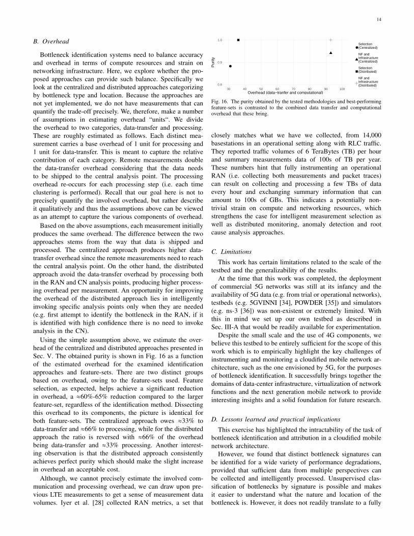
B. Overhead
Bottleneck identification systems need to balance accuracyand overhead in terms of compute resources and strain onnetworking infrastructure. Here, we explore whether the pro-posed approaches can provide such balance. Specifically welook at the centralized and distributed approaches categorizingby bottleneck type and location. Because the approaches arenot yet implemented, we do not have measurements that canquantify the trade-off precisely. We, therefore, make a numberof assumptions in estimating overhead “units“. We dividethe overhead to two categories, data-transfer and processing.These are roughly estimated as follows. Each distinct mea-surement carries a base overhead of 1 unit for processing and1 unit for data-transfer. This is meant to capture the relativecontribution of each category. Remote measurements doublethe data-transfer overhead considering that the data needsto be shipped to the central analysis point. The processingoverhead re-occurs for each processing step (i.e. each timeclustering is performed). Recall that our goal here is not toprecisely quantify the involved overhead, but rather describeit qualitatively and thus the assumptions above can be viewedas an attempt to capture the various components of overhead.
Based on the above assumptions, each measurement initiallyproduces the same overhead. The difference between the twoapproaches stems from the way that data is shipped andprocessed. The centralized approach produces higher data-transfer overhead since the remote measurements need to reachthe central analysis point. On the other hand, the distributedapproach avoid the data-transfer overhead by processing bothin the RAN and CN analysis points, producing higher process-ing overhead per measurement. An opportunity for improvingthe overhead of the distributed approach lies in intelligentlyinvoking specific analysis points only when they are needed(e.g. first attempt to identify the bottleneck in the RAN, if itis identified with high confidence there is no need to invokeanalysis in the CN).
Using the simple assumption above, we estimate the over-head of the centralized and distributed approaches presented inSec. V. The obtained purity is shown in Fig. 16 as a functionof the estimated overhead for the examined identificationapproaches and feature-sets. There are two distinct groupsbased on overhead, owing to the feature-sets used. Featureselection, as expected, helps achieve a significant reductionin overhead, a ≈60%-65% reduction compared to the largerfeature-set, regardless of the identification method. Dissectingthis overhead to its components, the picture is identical forboth feature-sets. The centralized approach owes ≈33% todata-transfer and ≈66% to processing, while for the distributedapproach the ratio is reversed with ≈66% of the overheadbeing data-transfer and ≈33% processing. Another interest-ing observation is that the distributed approach consistentlyachieves perfect purity which should make the slight increasein overhead an acceptable cost.
Although, we cannot precisely estimate the involved com-munication and processing overhead, we can draw upon pre-vious LTE measurements to get a sense of measurement datavolumes. Iyer et al. [28] collected RAN metrics, a set that
●
0.8
0.9
1.0
30 40 50 60 70 80 90 100Overhead (data−tranfer and computational)
Pur
ity
●Selection (Centralized)
NF and Infrastructure(Centralized)
Selection(Distributed)
NF and Infrastructure(Distributed)
Fig. 16. The purity obtained by the tested methodologies and best-performingfeature-sets is contrasted to the combined data transfer and computationaloverhead that these bring.
closely matches what we have we collected, from 14,000basestations in an operational setting along with RLC traffic.They reported traffic volumes of 6 TeraBytes (TB) per hourand summary measurements data of 100s of TB per year.These numbers hint that fully instrumenting an operationalRAN (i.e. collecting both measurements and packet traces)can result on collecting and processing a few TBs of dataevery hour and exchanging summary information that canamount to 100s of GBs. This indicates a potentially non-trivial strain on compute and networking resources, whichstrengthens the case for intelligent measurement selection aswell as distributed monitoring, anomaly detection and rootcause analysis approaches.
C. Limitations
This work has certain limitations related to the scale of thetestbed and the generalizability of the results.
At the time that this work was completed, the deploymentof commercial 5G networks was still at its infancy and theavailability of 5G data (e.g. from trial or operational networks),testbeds (e.g. 5GVINNI [34], POWDER [35]) and simulators(e.g. ns-3 [36]) was non-existent or extremely limited. Withthis in mind we set up our own testbed as described inSec. III-A that would be readily available for experimentation.
Despite the small scale and the use of 4G components, webelieve this testbed to be entirely sufficient for the scope of thiswork which is to empirically highlight the key challenges ofinstrumenting and monitoring a cloudified mobile network ar-chitecture, such as the one envisioned by 5G, for the purposesof bottleneck identification. It successfully brings together thedomains of data-center infrastructure, virtualization of networkfunctions and the next generation mobile network to provideinteresting insights and a solid foundation for future research.
D. Lessons learned and practical implications
This exercise has highlighted the intractability of the task ofbottleneck identification and attribution in a cloudified mobilenetwork architecture.
However, we found that distinct bottleneck signatures canbe identified for a wide variety of performance degradations,provided that sufficient data from multiple perspectives canbe collected and intelligently processed. Unsupervised clas-sification of bottlenecks by signature is possible and makesit easier to understand what the nature and location of thebottleneck is. However, it does not readily translate to a fully
15
automated system. While in this work we were in controlof the bottleneck profiles, understanding the classification ofbottlenecks encountered in the wild, in an operational networkwill require further intervention (e.g. labeling of anomalies).The success of unsupervised learning in telling apart differ-ent bottlenecks is encouraging and suggests that a properlytrained and tuned supervised classifier can potentially yieldperfect results. Training such models in a dynamic networkremains challenging and an interesting research direction.Multi-layered methodologies can also be envisioned where fastanomaly detection [37] is the first line of defence, while bot-tleneck localization and identification is deferred to secondaryanalysis. We also find that a centralized monitoring systemcan face difficulties when encountering complex bottlenecks.While methods for concurrently identifying multiple bottle-necks exist, the distributed architecture can naturally tacklethe task from multiple points of view while maintaining alow overhead, giving it a notable edge. However, designingan efficient distributed monitoring system mandates solvinga number of key problems. These include the distributiongranularity and how to coordinate between its compartments.The finer the granularity the better the system at attributingcomposite bottlenecks. A finer granularity however, wouldcomplicate the task of coordinating between the differentcompartments in the system and may impact the timelinessof bottleneck identification. We plan to explore these tradeoffs in our future work.
VIII. RELATED WORK
Based on our analysis and efforts in bottleneck identificationthere is strong evidence that holistic cross-layer monitoringsolutions, exploiting a rich set of monitoring data are of greatimportance for identifying potential bottlenecks and providingservice performance guarantees in the emerging cloudifiedmobile systems. However, considering the state of the art inthe monitoring space, we can observe a disparity in the waythat the problem is dealt with depending on the domain, bothin terms of industrial solutions and the research literature.
In the domains of cloud computing and data centers, aplethora of practical monitoring systems already exist, eithertailored for specific environments (e.g. Microsoft’s AzureMonitor [38] for the Azure cloud) or targeting more genericinfrastructure deployments, like Zabbix [39] and Nagios [40].Such systems allow the monitoring of KPIs like CPU/networkutilization, memory/storage usage, network flow informationetc, both in terms of the underlying physical infrastructureand of the deployed virtual network functions and support thetriggering of events and alarms whenever certain importantKPIs cross some threshold. In accordance to this, the focus ofresearch works in this space is on solutions that can make themonitoring of the relevant resources as efficient and as finegrained as possible, either from the angle of cloud computing(e.g. [2]) or from the angle of the data center and the efficientmonitoring of network flows (e.g. [3], [41]). However, inall these cases monitoring is treated generically, not takinginto consideration domain specific monitoring informationoriginating at the network function and service layers, which
as shown in Sections IV and V, can improve the identificationof the root cause of performance bottlenecks.
In an analogous manner, monitoring solutions exist in themobile domain, like Nokia’s Wireless Network Guardian [42]and Amdocs’ Deep Network Analytics [43]. In contrast to thecloud solutions, these focus on analyzing data from the mobilenetworking domain such as RAN and CN related informationlike the ones in this work, to identify potential bottlenecks. Inthis case, the type of bottlenecks that are being considered aredifferent in nature and revolve around service-related issues,like interference, sudden traffic surges, etc. This focus canalso be seen in the research literature, with some examplesbeing [4], [44], which propose ways of exploiting mobilenetwork information to identify bottlenecks in real-time.
A number of new proprietary products are starting to appearthat attempt to fuse data from both domains (e.g. Ericsson’sNetwork Manager [45]). Similarly, both ETSI OSM [46] andONAP [47], the most prominent solutions for the managementand orchestration of cloudified mobile networks, provide sub-systems that can enable multi-source monitoring.
There is a fair amount of previous work on bottleneckcharacterization and monitoring of traditional mobile networks(e.g. [4], [28], [48]) and cloud computing infrastructures(e.g. [2], [3], [41], [49]–[51]). Equally, there is work onbottleneck characterization in virtualized mobile networks butfocusing solely on the CN (e.g. [52]–[54]).
On the side of advanced monitoring intelligence, z-TORCH [5], is an automated NFV orchestration and mon-itoring solution for generic virtual network functions thatprovides an adaptive monitoring mechanism in terms of thedata collection frequency, and attempts to profile the behaviorof VNFs. On a parallel path, [29], examines the trade-offof latency and accuracy in the domain of mobile analytics,focusing on the RAN.
To the best of our knowledge, there is no work thatseeks to holistically and experimentally examine the range ofperformance bottlenecks that can impact service quality in acloudified mobile network setting along with the measurementparameters that can help identify them. While capturing multi-layer data is already possible, the exact type of data thatshould be captured at any point in time and their monitoringfrequency is still unclear. Moreover, as our analysis showed,the link between cause and effect of performance degradationbecomes fuzzier due to the complexity of the network andthe virtualization of mobile network functions, complicatingthe monitoring process further. Also, naive approaches tocentrally collecting all monitoring data are unlikely to scalein operational networks [55]–[58].
In order to resolve the aforementioned challenges, a moreintelligent monitoring solution is required, that draws a balancein terms of scalability and accuracy of identifying bottlenecksthat lead to QoS degradation. Exploiting insights like the onesobtained in Sections IV and V regarding the usefulness of thevarious features is a good step towards this direction.
An effective framework targeting performance assurance ina cloudified mobile network context, should build on suchideas and expand their scope to capture all of the aspectssolidified by the 5G system architecture, including both the
16
domains of cloud computing and mobile networks and theidiosyncrasies of the individual network functions that areinvolved.
IX. CONCLUSIONS
In this work, we have presented an experimental studywith the goal of characterizing cloudified mobile networkperformance bottlenecks and explored the challenges in identi-fying them. To achieve this, we employed a prototype testbedthat allows the creation of end-to-end mobile network slicesthrough the NFV paradigm. Our experiments demonstrated thecomplexity involved in identifying such bottlenecks even forsimple scenarios and revealed how obtaining monitoring datafrom various layers of the cloudified ecosystem can improvethis identification process. Based on the insights gained fromthis exercise and considering the currently available monitor-ing solutions, it is clear that a novel and more intelligent mon-itoring framework is required for the assurance of 5G serviceperformance guarantees, taking into consideration both the ac-curacy of identifying bottlenecks and the overhead of monitor-ing. This is exemplified by the consideration of complex sce-narios featuring composite bottlenecks. Our evaluations showthat a decentralized bottleneck identification approach offershigh accuracy while keeping overhead reasonable. Designing amonitoring system that meets the aforementioned requirementsand expanding our current experimentation framework to cap-ture more complex bottlenecks with more types of monitoringdata are two important dimensions to consider in our futurework.
REFERENCES
[1] 5GPPP Architecture Working Group, “View on 5G Architecture,” WhitePaper, 2017.
[2] J. M. A. Calero and J. G. Aguado, “MonPaaS: an adaptive monitoringplatform as a service for cloud computing infrastructures and services,”IEEE Transactions on Services Computing, vol. 8, no. 1, pp. 65–78,2015.
[3] M. Moshref et al., “Trumpet: Timely and precise triggers in datacenters,” in Proceedings of the 2016 ACM SIGCOMM Conference.ACM, 2016, pp. 129–143.
[4] N. Baranasuriya, V. Navda, V. N. Padmanabhan, and S. Gilbert,“QProbe: locating the bottleneck in cellular communication,” in Pro-ceedings of the 11th ACM Conference on Emerging Networking Exper-iments and Technologies. ACM, 2015, p. 33.
[5] V. Sciancalepore et al., “z-TORCH: An Automated NFV Orchestrationand Monitoring Solution,” IEEE Transactions on Network and ServiceManagement, 2018.
[6] NGMN Alliance, “5G White Paper,” Feb 2015.[7] ITU-R, “IMT Vision – Framework and overall objectives of the future
development of IMT for 2020 and beyond,” Sept 2015.[8] X. Foukas, G. Patounas, A. Elmokashfi, and M. K. Marina, “Network
Slicing in 5G: Survey and Challenges,” IEEE Communications Maga-zine, vol. 55, no. 5, 2017.
[9] X. Foukas et al., “Orion: RAN Slicing for a Flexible and Cost-EffectiveMulti-Service Mobile Network Architecture,” in Proceedings of the 23rdACM MobiCom. ACM, 2017, pp. 127–140.
[10] N. Nikaein et al., “OpenAirInterface: A flexible platform for 5Gresearch,” ACM SIGCOMM CCR, vol. 44, no. 5, pp. 33–38, 2014.
[11] Eurecom, “Openair-CN,” https://gitlab.eurecom.fr/oai/openair-cn, 2018,accessed: 2018-10-10.
[12] X. Foukas et al., “Experience Building a Prototype 5G Testbed,” inProceedings of the 1st International Workshop on Experimentation andMeasurements in 5G (EM-5G). ACM, 2018.
[13] SDxCentral, “T-mobile 4G network,” https://www.sdxcentral.com/articles/news/rakuten-mobile-plans-commercial-4g-lte-launch-in-april/2020/01/, 2020, accessed: 2020-06-20.
[14] ——, “Rakuten Mobile 4G network,” https://www.sdxcentral.com/articles/news/t-mobile-poland-first-to-deploy-onf-open-source-epc/2020/01/, 2020, accessed: 2020-06-20.
[15] G. T. 21.915, “Release description; Release 15,” 2017.[16] G. Boudreau, J. Panicker, N. Guo, R. Chang, N. Wang, and S. Vrzic,
“Interference coordination and cancellation for 4G networks,” IEEECommunications Magazine, vol. 47, no. 4, 2009.
[17] D. Lopez-Perez, I. Guvenc, G. De la Roche, M. Kountouris, T. Q. Quek,and J. Zhang, “Enhanced intercell interference coordination challengesin heterogeneous networks,” IEEE Wireless communications, vol. 18,no. 3, 2011.
[18] The GNU Radio Foundation, “GNURadio,” https://www.gnuradio.org/,2018, accessed: 2018-10-15.
[19] X. Wu, D. Turner, G. Chen, D. Maltz, X. Yang, L. Yuan, andM. Zhang, “NetPilot: Automating Datacenter Network FailureMitigation,” in ACM SIGCOMM. ACM SIGCOMM, August2012. [Online]. Available: https://www.microsoft.com/en-us/research/publication/netpilot-automating-datacenter-network-failure-mitigation/
[20] Linux Network Developers , “Netem,” https://wiki.linuxfoundation.org/networking/netem, 2018, accessed: 2018-10-15.
[21] I. F. Akyildiz, P. Wang, and S.-C. Lin, “SoftAir: A software definednetworking architecture for 5G wireless systems,” Computer Networks,vol. 85, pp. 1–18, 2015.
[22] ESnet / Lawrence Berkeley National Laboratory, “iPerf3,” https://iperf.fr/, 2018, accessed: 2018-10-15.
[23] N. G. Bachiega, P. S. Souza, S. M. Bruschi, and S. d. R. de Souza,“Container-Based Performance Evaluation: A Survey and Challenges,”in Cloud Engineering (IC2E), 2018 IEEE International Conference on.IEEE, 2018, pp. 398–403.
[24] C. Zhao, Y. Wu, Z. Ren, W. Shi, Y. Ren, and J. Wan, “Quantifyingthe isolation characteristics in container environments,” in IFIP Inter-national Conference on Network and Parallel Computing. Springer,2017, pp. 145–149.
[25] A. Waterland, “Stress workload generator,” https://people.seas.harvard.edu/~apw/stress/, 2018, accessed: 2018-10-15.
[26] A. Botta, A. Dainotti, and A. Pescapè, “A tool for the generationof realistic network workload for emerging networking scenarios,”Computer Networks, vol. 56, no. 15, pp. 3531–3547, 2012.
[27] S. Godard, “Performance monitoring tools for Linux,” https://github.com/sysstat/sysstat, 2018, accessed: 2018-10-15.
[28] A. P. Iyer, L. E. Li, and I. Stoica, “Automating Diagnosis of CellularRadio Access Network Problems,” in Proceedings of the 23rd AnnualInternational Conference on Mobile Computing and Networking. ACM,2017, pp. 79–87.
[29] A. Padmanabha Iyer, L. Erran Li, M. Chowdhury, and I. Stoica,“Mitigating the latency-accuracy trade-off in mobile data analyticssystems,” in Proceedings of the 24th Annual International Conferenceon Mobile Computing and Networking, ser. MobiCom ’18. NewYork, NY, USA: ACM, 2018, pp. 513–528. [Online]. Available:http://doi.acm.org/10.1145/3241539.3241581
[30] H. Schütze, C. D. Manning, and P. Raghavan, Introduction to informa-tion retrieval. Cambridge University Press, 2008, vol. 39.
[31] S.-H. Cha, “Comprehensive survey on distance/similarity measuresbetween probability density functions,” City, vol. 1, no. 2, p. 1, 2007.
[32] J. H. Friedman et al., “Multivariate adaptive regression splines,” Theannals of statistics, vol. 19, no. 1, pp. 1–67, 1991.
[33] J. C. Bezdek, R. Ehrlich, and W. Full, “Fcm: The fuzzy c-meansclustering algorithm,” Computers & Geosciences, vol. 10, no. 2-3, pp.191–203, 1984.
[34] 5G-VINNI consortium, “5G-VINNI,” https://www.5g-vinni.eu/, 2019,accessed: 2019-11-26.
[35] The University of Utah, “Platform for Open Wireless Data-driven Ex-perimental Research,” https://powderwireless.net/, 2019, accessed: 2019-07-28.
[36] NS-3 Consortium, “ns-3 network simulator,” https://www.nsnam.org/,2019, accessed: 2019-11-26.
[37] M. Ahmed, A. N. Mahmood, and J. Hu, “A survey of network anomalydetection techniques,” Journal of Network and Computer Applications,vol. 60, pp. 19–31, 2016.
[38] Microsoft, “Azure Monitor,” https://docs.microsoft.com/en-us/azure/azure-monitor/overview, 2018, accessed: 2018-10-15.
[39] Zabbix, “Zabbix,” https://www.zabbix.com/, 2018, accessed: 2018-10-15.
[40] Nagios Open Source, “Nagios,” https://www.nagios.org/, 2018, accessed:2018-10-15.
[41] Y. Li et al., “FlowRadar: A Better NetFlow for Data Centers.” in NSDI,2016, pp. 311–324.
17
[42] Nokia, “Nokia Wireless Network Guardian,” https://networks.nokia.com/products/wireless-network-guardian, 2018, accessed: 2018-10-15.
[43] Amdocs, “Amdocs Deep Network Analytics,” https://tinyurl.com/ya6ausmh, 2018, accessed: 2018-10-15.
[44] A. P. Iyer, L. E. Li, and I. Stoica, “CellIQ: Real-Time Cellular NetworkAnalytics at Scale.” in NSDI, 2015, pp. 309–322.
[45] Ericsson, “Ericsson Network Manager,” https://www.ericsson.com/ourportfolio/network-management/network-manager, 2018, accessed:2018-10-15.
[46] ETSI, OSM, “Open Source MANO,” OSM home page, 2016.[47] ONAP, “ONAP,” https://www.onap.org/, 2018, accessed: 2018-10-15.[48] P. Rengaraju, C.-H. Lung, F. R. Yu, and A. Srinivasan, “On QoE
monitoring and E2E service assurance in 4G wireless networks,” IEEEWireless Communications, vol. 19, no. 4, 2012.
[49] L. Cao, P. Sharma, S. Fahmy, and V. Saxena, “NFV-VITAL: A frame-work for characterizing the performance of virtual network functions,” inNetwork Function Virtualization and Software Defined Network (NFV-SDN), 2015 IEEE Conference on. IEEE, 2015, pp. 93–99.
[50] P. Naik, D. K. Shaw, and M. Vutukuru, “NFVPerf: Online performancemonitoring and bottleneck detection for NFV,” in Network FunctionVirtualization and Software Defined Networks (NFV-SDN), IEEE Con-ference on. IEEE, 2016, pp. 154–160.
[51] S. Kandula, R. Mahajan, P. Verkaik, S. Agarwal, J. Padhye, andP. Bahl, “Detailed diagnosis in enterprise networks,” in Proceedings ofthe ACM SIGCOMM 2009 Conference on Data Communication, ser.SIGCOMM ’09. New York, NY, USA: ACM, 2009, pp. 243–254.[Online]. Available: http://doi.acm.org/10.1145/1592568.1592597
[52] A. S. Rajan, S. Gobriel, C. Maciocco, K. B. Ramia, S. Kapury,A. Singhy, J. Ermanz, V. Gopalakrishnanz, and R. Janaz, “Understandingthe bottlenecks in virtualizing cellular core network functions,” in Localand Metropolitan Area Networks (LANMAN), 2015 IEEE InternationalWorkshop on. IEEE, 2015, pp. 1–6.
[53] J. Prados-Garzon, J. J. Ramos-Munoz, P. Ameigeiras, P. Andres-Maldonado, and J. M. Lopez-Soler, “Modeling and dimensioning ofa virtualized MME for 5G mobile networks,” IEEE Transactions onVehicular Technology, vol. 66, no. 5, pp. 4383–4395, 2017.
[54] M. T. Raza, D. Kim, K.-H. Kim, S. Lu, and M. Gerla, “Rethinking LTEnetwork functions virtualization,” in Network Protocols (ICNP), 2017IEEE 25th International Conference on. IEEE, 2017, pp. 1–10.
[55] S. Meng, L. Liu, and T. Wang, “State monitoring in cloud datacenters,”IEEE transactions on Knowledge and Data Engineering, vol. 23, no. 9,pp. 1328–1344, 2011.
[56] S. Meng, A. K. Iyengar, I. M. Rouvellou, L. Liu, K. Lee, B. Palanisamy,and Y. Tang, “Reliable state monitoring in cloud datacenters,” in 2012IEEE Fifth International Conference on Cloud Computing. IEEE, 2012,pp. 951–958.
[57] J. Povedano-Molina, J. M. Lopez-Vega, J. M. Lopez-Soler, A. Corradi,and L. Foschini, “Dargos: A highly adaptable and scalable monitoringarchitecture for multi-tenant clouds,” Future Generation Computer Sys-tems, vol. 29, no. 8, pp. 2041–2056, 2013.
[58] ONAP, “DCAE: Multi-Site deployment options,” https://wiki.onap.org/display/DW/DCAE%3A+Multi-Site+deployment+options, 2020, ac-cessed: 2020-06-20.


![Cloning and Characterization of Two NAD Kinases from ... · Cloning and Characterization of Two NAD Kinases from Arabidopsis. Identification of a Calmodulin Binding Isoform1[w] William](https://img.pdfslide.us/doc/110x75/5c346b1109d3f2f3288bfa5c/cloning-and-characterization-of-two-nad-kinases-from-cloning-and-characterization.jpg)

![Identification and Characterization of Maize oury4 …Identification and Characterization of Maizefloury4 as a Novel Semidominant Opaque Mutant That Disrupts Protein Body Assembly1[W][OPEN]](https://img.pdfslide.us/doc/110x75/5e4a4e7897d31144b35737e6/identiication-and-characterization-of-maize-oury4-identiication-and-characterization.jpg)