Embed Size (px)
Citation preview
Discrete Comput Geom (2012) 48:915–963DOI 10.1007/s00454-012-9459-8
Characteristics of Graph Braid Groups
Ki Hyoung Ko · Hyo Won Park
Received: 30 June 2011 / Revised: 5 June 2012 / Accepted: 6 September 2012 /Published online: 25 September 2012© Springer Science+Business Media, LLC 2012
Abstract We give formulae for the first homology of the n-braid group and the pure2-braid group over a finite graph in terms of graph-theoretic invariants. As immediateconsequences, a graph is planar if and only if the first homology of the n-braid groupover the graph is torsion-free and the conjectures about the first homology of the pure2-braid groups over graphs in Farber and Hanbury (arXiv:1005.2300 [math.AT]) canbe verified. We discover more characteristics of graph braid groups: the n-braid groupover a planar graph and the pure 2-braid group over any graph have a presentationwhose relators are words of commutators, and the 2-braid group and the pure 2-braidgroup over a planar graph have a presentation whose relators are commutators. Thelatter was a conjecture in Farley and Sabalka (J. Pure Appl. Algebra, 2012) and sowe propose a similar conjecture for higher braid indices.
Keywords Braid group · Configuration space · Graph · Homology · Presentation
1 Introduction
Given a topological space Γ , let CnΓ and UCnΓ , respectively, denote the orderedand unordered configuration spaces of n-points in Γ . That is,
CnΓ = {(x1, . . . , xn) ∈ Γ n | xi �= xj if i �= j}
and
UCnΓ = {{x1, . . . , xn} ⊂ Γ | xi �= xj if i �= j}.
K.H. Ko (�) · H.W. ParkDepartment of Mathematics, Korea Advanced Institute of Science and Technology, Daejeon,307-701, Koreae-mail: [email protected]
H.W. Parke-mail: [email protected]
916 Discrete Comput Geom (2012) 48:915–963
By considering the symmetric group Sn permuting n coordinates in Γ n, UCnΓ isidentified with the quotient space CnΓ/Sn.
In this article, we assume Γ is a finite connected graph regarded as a Euclideansubspace and we study topological characteristics, in particular their homologies andfundamental groups, of CnΓ and UCnΓ via graph-theoretical characteristics of Γ .
Instead of the configuration spaces CnΓ and UCnΓ that have open boundaries, itis convenient to use their cubical complex alternatives—the ordered discrete configu-ration space Dn and the unordered discrete configuration space UDn. After regardingΓ as a 1-dimensional CW complex, we define
DnΓ = {(c1, . . . , cn) ∈ Γ n | ∂ci ∩ ∂cj = ∅ if i �= j}
and
UDnΓ = {{c1, . . . , cn} ⊂ Γ | ∂ci ∩ ∂cj = ∅ if i �= j}
where ci is either a 0-cell (or vertex) or an open 1-cell (or edge) in Γ and ∂ci denoteseither ci itself if ci is a 0-cell or its ends if ci is an open 1-cell.
If Γ is suitably subdivided in the sense that each path between two vertices ofvalency �= 2 contains at least n− 1 edges and each simple loop at a vertex contains atleast n+ 1 edges, then according to [1, 12, 14], the discrete configuration space DnΓ
(UDnΓ , respectively) is deformation retract of the usual configuration space CnΓ
(UCnΓ , respectively). Under the assumption of suitable subdivision, the pure graphbraid group PnΓ and the graph braid group BnΓ of Γ are the fundamental groupsof the ordered and the unordered configuration spaces of Γ , that is,
PnΓ = π1(CnΓ ) ∼= π1(DnΓ ) and BnΓ = π1(UCnΓ ) ∼= π1(UDnΓ ).
Abrams showed in [1] that discrete configuration spaces DnΓ and UDnΓ are cubi-cal complexes of nonpositive curvature and so locally CAT(0) spaces. In particular,DnΓ and UDnΓ are Eilenberg–MacLane spaces, and PnΓ and BnΓ are torsion-free.Furthermore,
Hi(PnΓ ) ∼= Hi(CnΓ ) ∼= Hi(DnΓ ) and Hi(BnΓ ) ∼= Hi(UCnΓ ) ∼= Hi(UDnΓ ).
Conceiving applications to robotics, Abrams and Ghrist [2] around 2000 beganto study configuration spaces over graphs and graph braid groups from the topolog-ical point of view. Research on graph braid groups has mainly been concentrated oncharacteristics of their presentations. An outstanding question was which graph braidgroup is a right-angled Artin group. The precise characterization of such graphs wasgiven in [12] for n ≥ 5 by extending the result in [8] for trees and n ≥ 4. So it isnatural to consider two other classes of groups defined by relaxing the requirementof right-angled Artin groups that have a presentation whose relators are commutatorsof generators. A simple-commutator-related group has a presentation whose relatorsare commutators, and a commutator-related group has a presentation whose relatorsare words of commutators. Farley and Sabalka proved in [9] that B2Γ is simple-commutator-related if every pair of cycles in Γ are disjoint and they conjectured thatB2Γ are simple-commutator-related whose relators are related to two disjoints cyclesif Γ is planar.
Discrete Comput Geom (2012) 48:915–963 917
On the other hand, Farley showed in [6] that the homology groups of the unorderedconfiguration space UCnT for a tree T are torsion-free and computed their ranks.Kim, Ko and Park proved that if Γ is non-planar, H1(UCnΓ ) has a 2-torsion and theconverse holds for n = 2, and they conjectured that H1(BnΓ ) is torsion-free iff Γ
is planar [12]. Barnett and Farber showed in [3] that for a planar graph Γ satisfyinga certain condition (which implies that Γ is either the Θ-shape graph or a simpleand triconnected graph), β1(C2Γ ) = 2β1(Γ ) + 1. Furthermore, Farber and Hanburyshowed in [10] that for a non-planar graph Γ satisfying a certain condition (whichalso implies that Γ is a simple and triconnected graph), β1(C2Γ ) = 2β1(Γ ). Theyalso conjectured that H1(C2Γ ) is always torsion-free and that β1(C2Γ ) = 2β1(Γ ) iffΓ is non-planar, simple and triconnected (this is equivalent to their hypothesis).
In this article, we express H1(UCnΓ ) and H1(C2Γ ) for an finite connectedgraph Γ in terms of graph-theoretic invariants (see Theorems 3.16 and 3.25). Allthe results and the conjectures, mentioned above, on the first homologies of con-figuration spaces over graphs are immediate consequences of these expressions. Inaddition, we prove that BnΓ is commutator-related for a planar graph Γ and P2Γ isalways commutator-related (see Theorem 4.6). By combining with a result of [3], wefinally prove that for a planar graph Γ , B2Γ and P2Γ are simple-commutator-relatedwhose relators are commutators of words corresponding to pairs of disjoint cycles onΓ (see Theorem 4.8).
The major tool for computing H1(UCnΓ ) is to use a Morse complex of UDnΓ
obtained via discrete Morse theory. In Sect. 2, we first give an example that illus-trates how to use the Morse complex to compute H1(UCnΓ ). Then we choose a nicemaximal tree of Γ and its planar embedding, the second boundary map of the Morsecomplex induced from these choices becomes so manageable that a description of thesecond boundary map can be given.
In Sect. 3, the matrix for the second boundary map is systematically simplified (seeTheorem 3.5) via row operations after giving certain orders on generating 1-cells and2-cells (called critical cells) of the Morse complex. Then we decompose Γ into bi-connected graphs and further decompose each biconnected graph into triconnectedgraphs and compute the contribution from critical 1-cells that disappear under thesedecompositions. Then we show all critical 1-cells except those coming from deletededges are homologous up to signs for a given triconnected graph and generate a sum-mand Z or Z2 depending on whether the graph is planar or not. Finally we collectresults from all decompositions to have a formula for H1(UCnΓ ). For n = 2, the sec-ond boundary map of the Morse complex of DnΓ is not any harder than the Morsecomplex of UDnΓ . Thus the formula for H1(C2Γ ) is obtained by a similar argument.
In Sect. 4, we develop noncommutative versions of some of technique in the pre-vious section to obtain optimized presentations of (pure) graph braid groups so thatthey have certain desired properties via Tietze transformation. In fact, the orders oncritical 1-cells and 2-cells play crucial roles in systematic eliminations of cancelingpairs of a 2-cell and a 1-cell. And we show that (pure) graph braid groups have pre-sentations with special characteristics mentioned above. We finish the paper with theconjecture about a graph Γ such that BnΓ and P3Γ are simple-commutator-relatedgroups.
918 Discrete Comput Geom (2012) 48:915–963
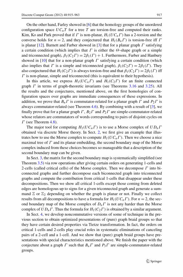
Fig. 1 Choose a maximal tree and give an order
2 Discrete Configuration Spaces and Discrete Morse Theory
Given a finite graph Γ , the unordered discrete configuration space UDnΓ is col-lapsed to a complex called a Morse complex by using discrete Morse theory devel-oped by Forman [11]. In Sect. 2.1, we briefly review this technology following [7, 12]and use it to compute H1(UD2K3,3) as a warm-up that demonstrates what is aheadfor us. In Sect. 2.2, we extend the technique to the discrete configuration space DnΓ
and compute H1(D2K3,3) as an example. In Sect. 2.3, we show how to choose anice maximal tree and its embedding so that the second boundary map of the inducedMorse complex can be described in the fewest possible cases. Then we list up all ofthese cases in a few lemmas.
2.1 Discrete Morse Theory on UDnΓ
Let Γ be a suitably subdivided graph. In order to collapse the unordered discreteconfiguration space UDnΓ via discrete Morse theory, we first choose a maximal treeT of Γ . Edges in Γ − T are called deleted edges. Pick a vertex of valency 1 in T asa base point and assign 0 to this vertex. We assume that the path between the basevertex 0 and the nearest vertex of valency ≥3 in T contains at least n − 1 edges forthe purpose that will be revealed later. Next we give an order on vertices as follows:Fix an embedding of T on the plane. Let R be a regular neighborhood of T . Startingfrom the base vertex 0, we number unnumbered vertices of T as we travel along ∂R
clockwise. Figure 1 illustrates this procedure for the complete bipartite graph K3,3and for n = 2. There are four deleted edges to form a maximal tree. All vertices in Γ
are numbered and so are referred by the nonnegative integers.Each edge e in Γ is oriented so that the initial vertex ι(e) is larger than the termi-
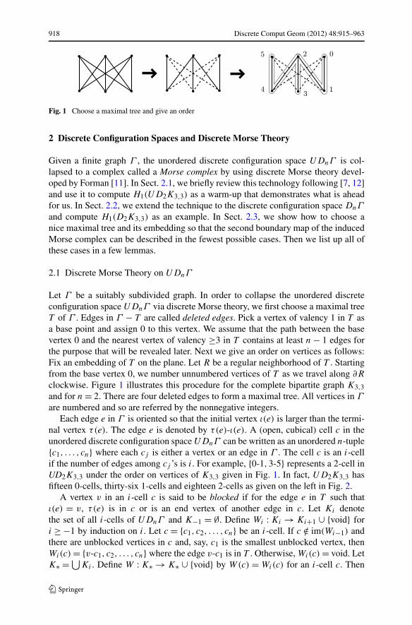
nal vertex τ(e). The edge e is denoted by τ(e)-ι(e). A (open, cubical) cell c in theunordered discrete configuration space UDnΓ can be written as an unordered n-tuple{c1, . . . , cn} where each cj is either a vertex or an edge in Γ . The cell c is an i-cellif the number of edges among cj ’s is i. For example, {0-1,3-5} represents a 2-cell inUD2K3,3 under the order on vertices of K3,3 given in Fig. 1. In fact, UD2K3,3 hasfifteen 0-cells, thirty-six 1-cells and eighteen 2-cells as given on the left in Fig. 2.
A vertex v in an i-cell c is said to be blocked if for the edge e in T such thatι(e) = v, τ(e) is in c or is an end vertex of another edge in c. Let Ki denotethe set of all i-cells of UDnΓ and K−1 = ∅. Define Wi : Ki → Ki+1 ∪ {void} fori ≥ −1 by induction on i. Let c = {c1, c2, . . . , cn} be an i-cell. If c /∈ im(Wi−1) andthere are unblocked vertices in c and, say, c1 is the smallest unblocked vertex, thenWi(c) = {v-c1, c2, . . . , cn} where the edge v-c1 is in T . Otherwise, Wi(c) = void. LetK∗ =⋃Ki . Define W : K∗ → K∗ ∪ {void} by W(c) = Wi(c) for an i-cell c. Then
Discrete Comput Geom (2012) 48:915–963 919
Fig. 2 UD2K3,3 and the map W
it is not hard to see that W is well-defined, and each cell in W(K∗) − {void} hasthe unique preimage under W , and there is no cell in K∗ that is both an image anda preimage of other cells under W . For example, each arrow on the right of Fig. 2points from c to W(c) in UD2K3,3 and the dashed lines represent 1-cells sent to voidunder W .
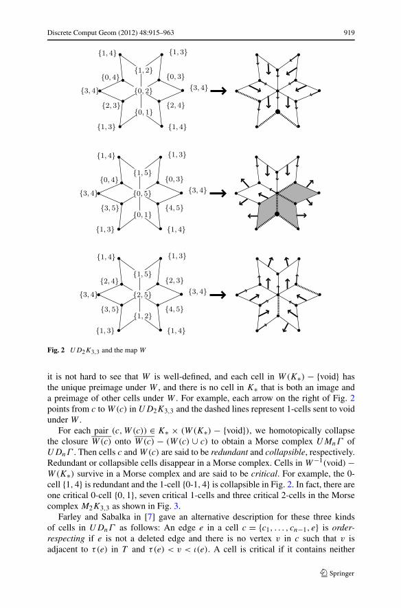
For each pair (c,W(c)) ∈ K∗ × (W(K∗) − {void}), we homotopically collapsethe closure W(c) onto W(c) − (W(c) ∪ c) to obtain a Morse complex UMnΓ ofUDnΓ . Then cells c and W(c) are said to be redundant and collapsible, respectively.Redundant or collapsible cells disappear in a Morse complex. Cells in W−1(void) −W(K∗) survive in a Morse complex and are said to be critical. For example, the 0-cell {1,4} is redundant and the 1-cell {0-1,4} is collapsible in Fig. 2. In fact, there areone critical 0-cell {0,1}, seven critical 1-cells and three critical 2-cells in the Morsecomplex M2K3,3 as shown in Fig. 3.
Farley and Sabalka in [7] gave an alternative description for these three kindsof cells in UDnΓ as follows: An edge e in a cell c = {c1, . . . , cn−1, e} is order-respecting if e is not a deleted edge and there is no vertex v in c such that v isadjacent to τ(e) in T and τ(e) < v < ι(e). A cell is critical if it contains neither
920 Discrete Comput Geom (2012) 48:915–963
Fig. 3 Morse complexUM2K3,3 of UD2K3,3
order-respecting edges nor unblocked vertices. A cell is collapsible if it contains atleast one order-respecting edge and each unblocked vertex is larger than the initialvertex of some order-respecting edge. A cell is redundant if it contains at least oneunblocked vertex that is smaller than the initial vertices of all order-respecting edges.Notice that there is exactly one critical 0-cell {0,1, . . . , n− 1} by the assumption thatthere are at least n− 1 edges between 0 and the nearest vertex with valency ≥3 in themaximal tree.
A choice of a maximal tree of Γ and its planar embedding determine an order onvertices and in turn a Morse complex UMnΓ that is homotopy equivalent to UDnΓ .We wish to compute its homology groups via the cellular structure of UMnΓ .
Let (Ci(UDnΓ ), ∂) be the (cubical) cellular chain complex of UDnΓ . For ani-cell c = {e1, e2, . . . , ei, vi+1, . . . , vn} of UDnΓ such that e1, . . . , ei are edges withτ(e1) < τ(e2) < · · · < τ(ei) and vi+1, . . . , vn are vertices of Γ , let
∂ιk(c) = {e1, . . . , ek−1, ek+1, . . . , ei, vi+1, . . . , vn, ι(ek)
},
∂τk (c) = {e1, . . . , ek−1, ek+1, . . . , ei , vi+1, . . . , vn, τ (ek)
}.
Then we define the boundary map as
∂(c) =i∑
k=1
(−1)k(∂ιk(c) − ∂τ
k (c)).
Notice that this definition of ∂ on UDnΓ is different from that in [7] and [12] insign convention. This convention seems more convenient in the current work. LetMi(UDnΓ ) be the free abelian group generated by critical i-cells. We now try toturn the graded abelian group {Mi(UDnΓ )} into a chain complex.
Let R : Ci(UDnΓ ) → Ci(UDnΓ ) be a homomorphism defined by R(c) = 0 ifc is a collapsible i-cell, by R(c) = c if c is critical, and by R(c) = ±∂W(c) + c
if c is redundant where the sign is chosen so that the coefficient of c in ∂W(c)
is −1. By [11], there is a nonnegative integer m such that Rm = Rm+1, andlet R = Rm. Then R(c) is in Mi(UDnΓ ) and we have a homomorphism R :Ci(UDnΓ ) → Mi(UDnΓ ). Define a map ∂ : Mi(UDnΓ ) → Mi−1(UDnΓ ) by∂(c) = R∂(c). Then (Mi(UDnΓ ), ∂) forms a chain complex. However, the inclusionM∗(UDnΓ ) ↪→ C∗(UDnΓ ) is not a chain map. Instead, consider a homomorphism
Discrete Comput Geom (2012) 48:915–963 921
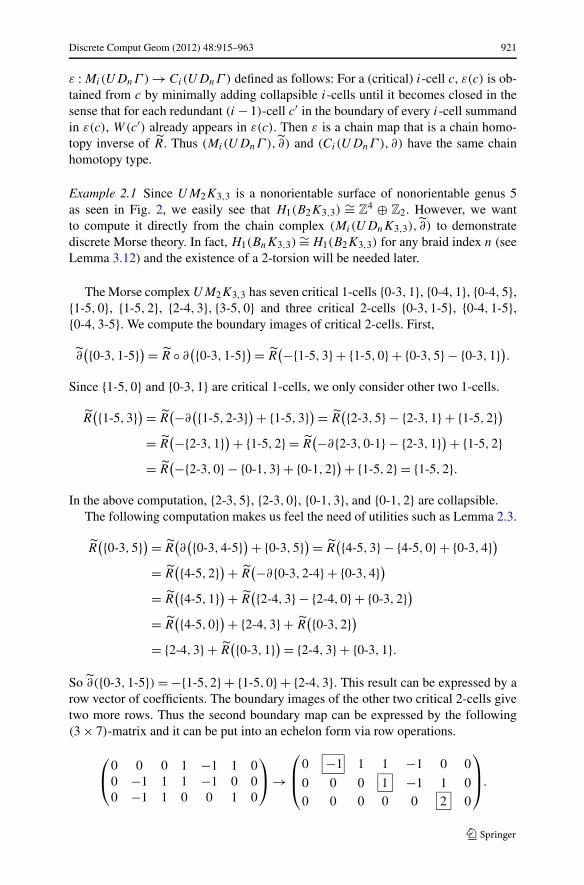
ε : Mi(UDnΓ ) → Ci(UDnΓ ) defined as follows: For a (critical) i-cell c, ε(c) is ob-tained from c by minimally adding collapsible i-cells until it becomes closed in thesense that for each redundant (i − 1)-cell c′ in the boundary of every i-cell summandin ε(c), W(c′) already appears in ε(c). Then ε is a chain map that is a chain homo-topy inverse of R. Thus (Mi(UDnΓ ), ∂) and (Ci(UDnΓ ), ∂) have the same chainhomotopy type.
Example 2.1 Since UM2K3,3 is a nonorientable surface of nonorientable genus 5as seen in Fig. 2, we easily see that H1(B2K3,3) ∼= Z
4 ⊕ Z2. However, we wantto compute it directly from the chain complex (Mi(UDnK3,3), ∂) to demonstratediscrete Morse theory. In fact, H1(BnK3,3) ∼= H1(B2K3,3) for any braid index n (seeLemma 3.12) and the existence of a 2-torsion will be needed later.
The Morse complex UM2K3,3 has seven critical 1-cells {0-3,1}, {0-4,1}, {0-4,5},{1-5,0}, {1-5,2}, {2-4,3}, {3-5,0} and three critical 2-cells {0-3,1-5}, {0-4,1-5},{0-4,3-5}. We compute the boundary images of critical 2-cells. First,
∂({0-3,1-5})= R ◦ ∂
({0-3,1-5})= R(−{1-5,3} + {1-5,0} + {0-3,5} − {0-3,1}).
Since {1-5,0} and {0-3,1} are critical 1-cells, we only consider other two 1-cells.
R({1-5,3})= R
(−∂({1-5,2-3})+ {1-5,3})= R
({2-3,5} − {2-3,1} + {1-5,2})
= R(−{2-3,1})+ {1-5,2} = R
(−∂{2-3,0-1} − {2-3,1})+ {1-5,2}= R(−{2-3,0} − {0-1,3} + {0-1,2})+ {1-5,2} = {1-5,2}.
In the above computation, {2-3,5}, {2-3,0}, {0-1,3}, and {0-1,2} are collapsible.The following computation makes us feel the need of utilities such as Lemma 2.3.
R({0-3,5})= R
(∂({0-3,4-5})+ {0-3,5})= R
({4-5,3} − {4-5,0} + {0-3,4})
= R({4-5,2})+ R
(−∂{0-3,2-4} + {0-3,4})
= R({4-5,1})+ R
({2-4,3} − {2-4,0} + {0-3,2})
= R({4-5,0})+ {2-4,3} + R
({0-3,2})
= {2-4,3} + R({0-3,1})= {2-4,3} + {0-3,1}.
So ∂({0-3,1-5}) = −{1-5,2} + {1-5,0} + {2-4,3}. This result can be expressed by arow vector of coefficients. The boundary images of the other two critical 2-cells givetwo more rows. Thus the second boundary map can be expressed by the following(3 × 7)-matrix and it can be put into an echelon form via row operations.
⎛
⎝0 0 0 1 −1 1 00 −1 1 1 −1 0 00 −1 1 0 0 1 0
⎞
⎠→⎛
⎜⎝
0 −1 1 1 −1 0 0
0 0 0 1 −1 1 00 0 0 0 0 2 0
⎞
⎟⎠.
922 Discrete Comput Geom (2012) 48:915–963
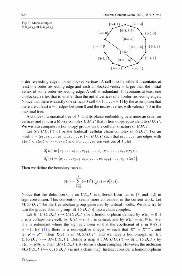
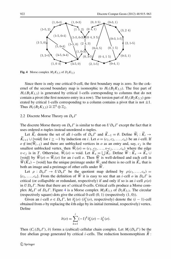
Fig. 4 Morse complex M2K3,3 of D2K3,3
Since there is only one critical 0-cell, the first boundary map is zero. So the cok-ernel of the second boundary map is isomorphic to H1(B2K3,3). The free part ofH1(B2K3,3) is generated by critical 1-cells corresponding to columns that do notcontain a pivot (the first nonzero entry in a row). The torsion part of H1(B2K3,3) gen-erated by critical 1-cells corresponding to a column contains a pivot that is not ±1.Thus H1(B2K3,3) ∼= Z
4 ⊕ Z2.
2.2 Discrete Morse Theory on DnΓ
The discrete Morse theory on DnΓ is similar to that on UDnΓ except the fact that ituses ordered n-tuples instead unordered n-tuples.
Let Ki denote the set of all i-cells of DnΓ and K−1 = ∅. Define Wi : Ki →Ki+1 ∪ {void} for i ≥ −1 by induction on i. Let o = (c1, c2, . . . , cn) be an i-cell. Ifo /∈ im(Wi−1) and there are unblocked vertices in o as an entry and, say, cj is thesmallest unblocked vertex, then Wi(o) = (c1, c2, . . . , v-cj , . . . , cn) where the edgev-cj is in T . Otherwise, Wi(o) = void. Let K∗ = ⋃ Ki . Define W : K∗ → K∗ ∪{void} by W (o) = Wi(o) for an i-cell o. Then W is well-defined and each cell inW (K∗) − {void} has the unique preimage under W , and there is no cell in K∗ that isboth an image and a preimage of other cells under W .
Let ρ : DnΓ → UDnΓ be the quotient map defined by ρ(c1, . . . , cn) ={c1, . . . , cn}. From the definition of W it is easy to see that an i-cell o in DnΓ iscritical (or collapsible or redundant, respectively) if and only if so is an i-cell ρ(o)
in UDnΓ . Note that there are n! critical 0-cells. Critical cells produce a Morse com-plex MnΓ of DnΓ . Figure 4 is a Morse complex M2K3,3 of D2K3,3. The circular(respectively square) dots give the critical 0-cell (0,1) (respectively (1,0)).
Given an i-cell o ∈ DnΓ , let ∂ιk(o) (∂τ
k (o), respectively) denote the (i − 1)-cellobtained from o by replacing the kth edge by its initial (terminal, respectively) vertex.Define
∂(o) =i∑
k=1
(−1)k∂ιk(o) − ∂τ
k (o).
Then (Ci(DnΓ ), ∂) forms a (cubical) cellular chain complex. Let Mi(DnΓ ) be thefree abelian group generated by critical i-cells. The reduction homomorphism R :
Discrete Comput Geom (2012) 48:915–963 923
Ci(DnΓ ) → Mi(DnΓ ) is also well-defined. For ∂ = R ◦ ∂ , (Mi(DnΓ ), ∂) forms aMorse chain complex that is chain homotopy equivalent to (Ci(DnΓ ), ∂).
In order to carry over some of computational results on UDnΓ to DnΓ , weintroduce a bookkeeping notation. Give an order among vertices and edges of Γ
by comparing the number assigned to vertices or terminal vertices of edges. De-fine a projection φ : DnΓ → Sn by sending o = (c1, . . . , cn) to the permutation σ
such that cσ(1) < · · · < cσ(n). And define a bijection Φ : DnΓ → UDnΓ × Sn byΦ(o) = (ρ(o),φ(o)). For example, Φ((1-3,2)) = ({1-3,2}, id) and Φ((4,3-5)) =({4,3-5}, (1,2)) where id is the identity permutation. The maps W , ∂ , R, and ∂ arecarried over to K∗ × Sn, C∗(UDnΓ ) × Sn, and M∗(UDnΓ ) × Sn by conjugatingwith Φ . For example, the ith boundary homomorphism on M∗(UDnΓ )×Sn is givenby Φ ◦ ∂ ◦ Φ−1. To make the notation more compact, an element (c, σ ) ∈ K∗ × Sn
will be denoted by cσ .
Example 2.2 Let Γ be K3,3 and a maximal tree and an order be given as in Fig. 1.We want to compute H1(P2K3,3) which will be used later.
From Fig. 4, one can see that H1(P2K3,3) ∼= Z8. But we want to demonstrate how
to compute H1(P2K3,3) using the Morse chain complex. Let σ be the permutation(1,2) ∈ S2. There are two critical 0-cells {0,1}id, {0,1}σ . There are fourteen criti-cal 1-cells {0-3,1}id, {0-3,1}σ , {0-4,1}id, {0-4,1}σ , {0-4,5}id, {0-4,5}σ , {1-5,0}id,{1-5,0}σ , {1-5,2}id, {1-5,2}σ , {2-4,3}id, {2-4,3}σ , {3-5,0}id, {3-5,0}σ and their im-age under ∂ is as follows:
∂({0-3,1}id
)= R(−{1,3}σ + {0,1}id
)= −{0,1}σ + {0,1}id
since R({1,3}σ ) = R(∂({0-1,3}σ ) + {1,3}σ ) = R({0,3}σ ) = · · · = {0,1}σ (seeLemma 3.18). So ∂({0-3,1}σ ) = −{0,1}id + {0,1}σ because of σ 2 = id. Similarlywe can compute images of critical 1-cells as follows:
∂({0-4,1}id
)= ∂({1-5,2}id
)= ∂({2-4,3}id
)= −{0,1}σ + {0,1}id
∂({0-4,5}id
)= ∂({1-5,0}id
)= ∂({3-5,0}id
)= 0.
There are six critical 2-cells {0-3,1-5}id, {0-3,1-5}σ , {0-4,1-5}id, {0-4,1-5}σ ,{0-4,3-5}id, {0-4,3-5}σ . We compute boundaries for the first two:
∂({0-3,1-5}id
)= R(−{1-5,3}σ + {1-5,0}id + {0-3,5}id − {0-3,1}id
).
Since {1-5,0}id and {0-3,1}id are critical 1-cells, we only consider other two 1-cells.
R({1-5,3}σ
)= R(−∂({1-5,2-3}σ
)+ {1-5,3}σ)
= R({2-3,5}id − {2-3,1}σ + {1-5,2}σ
)= {1-5,2}σsince R({2-3,1}) = 0 and no critical 1-cell appears in the process of computingR({2-3,1}) (see Example 2.1).
R({0-3,5}id
)= R({0-3,4}id
)= R(−∂({0-3,2-4}id
)+ {0-3,4}id)
924 Discrete Comput Geom (2012) 48:915–963
= R({2-4,3}σ − {2-4,0}id + {0-3,2}id
)
= {2-4,3}σ + R({0-3,1}id
)= {2-4,3}σ + {0-3,1}id.
So ∂({0-3,1-5}id) = −{1-5,2}σ + {1-5,0}id + {2-4,3}σ . This implies ∂({0-3,
1-5}σ ) = −{1-5,2}id + {1-5,0}σ + {2-4,3}id.Over these critical cells, the second boundary map is represented by the following
matrix.⎛
⎜⎜⎜⎜⎜⎜⎝
0 0 0 0 0 0 1 0 0 −1 0 1 0 00 0 0 0 0 0 0 1 −1 0 1 0 0 00 0 −1 0 1 0 1 0 0 −1 0 0 0 00 0 0 −1 0 1 0 1 −1 0 0 0 0 00 0 −1 0 1 0 0 0 0 0 1 0 0 00 0 0 −1 0 1 0 0 0 0 0 1 0 0
⎞
⎟⎟⎟⎟⎟⎟⎠
.
Since the kernel of the first boundary map is generated by either o or o ± {0-3,1}idfor all other critical 1-cells o, the matrix obtained from the above matrix by deletingthe first column is a presentation matrix of H1(P2K3,3). Using row operations on thepresentation matrix, we obtain the following echelon form.
⎛
⎜⎜⎜⎜⎜⎜⎜⎜⎝
0 −1 0 1 0 1 0 0 −1 0 0 0 0
0 0 −1 0 1 0 1 −1 0 0 0 0 0
0 0 0 0 0 −1 0 0 1 1 0 0 0
0 0 0 0 0 0 −1 1 0 0 1 0 0
0 0 0 0 0 0 0 0 0 1 1 0 00 0 0 0 0 0 0 0 0 0 0 0 0
⎞
⎟⎟⎟⎟⎟⎟⎟⎟⎠
.
Thus H1(P2K3,3) ∼= Z8.
2.3 The Second Boundary Homomorphism
To give a general computation of the second boundary homomorphism ∂ on a Morsecomplex, we first exhibit redundant 1-cells whose reductions are straightforward andthen explain how to choose a maximal tree of a given graph to take advantage of thesesimple reductions.
Let Γ be a graph and T be a maximal tree of Γ . Let c be a redundant i-cell inUDnΓ , v be an unblocked vertex in c and e be the edge in T starting from v. LetVe(c) denote the i-cell obtained from c by replacing v by τ(e). Define a functionV : Ki → Ki by V (c) = Ve(c) if c is redundant and ι(e) is the smallest unblockedvertex in c, and by V (c) = c otherwise. The function V should stabilize to a functionV : Ki → Ki under iteration, that is, V = V m for some nonnegative integer m suchthat V m = V m+1.
Lemma 2.3 (Kim–Ko–Park [12]) Let c be a redundant cell and v be an unblockedvertex. Suppose that for the edge e starting from v, there is no vertex w that is either inc or an end vertex of an edge in c and satisfies τ(e) < w < ι(e). Then R(c) = RVe(c).
Discrete Comput Geom (2012) 48:915–963 925
We continue to define more notation and terminology. For each vertex v in Γ , thereis a unique edge path γv from v to the base vertex 0 in T . For vertices v, w in Γ ,v ∧ w denotes the vertex that is the first intersection between γv and γw . Obviously,v ∧ w ≤ v and v ∧ w ≤ w. The number assigned to the branch of v occupied bythe path from v to w in T is denoted by g(v,w). If v = w ∧ v, g(v,w) ≥ 1 and ifv > w ∧ v, g(v,w) = 0. An edge e in Γ is said to be separated by a vertex v if ι(e)
and τ(e) lie in two distinct components of T −{v}. It is clear that only a deleted edgecan be separated by a vertex. If a deleted edge d is not separated by v, then ι(d),τ(d), and ι(d) ∧ τ(d) are all in the same component of T − {v}.
For redundant 1-cells, we can strengthen the above lemma as follows.
Lemma 2.4 (Special Reduction) Let c be a redundant 1-cell containing an edge p.Suppose the redundant 1-cell c has an unblocked vertex v and the edge e startingfrom v satisfies the following:
(a) Every vertex w in c satisfying τ(e) < w < ι(e) is blocked.(b) If an end vertex w of p satisfies τ(e) < w < ι(e) then p is not separated by τ(e).
Then R(c) = RVe(c). Therefore if p is not a deleted edge then R(c) = RV (c).
Proof Assume that both ends of p are not between τ(e) and ι(e). Since p is the onlyedge in c that can initiate a blockage, it is impossible to have a vertex between τ(e)
and ι(e) due to the condition (a). Then we are done by Lemma 2.3.Assume that an end of p is between τ(e) and ι(e). By the condition (b), both ι(p)
and τ(p) are in the same component Tp of T −{τ(e)} and are between τ(e) and ι(e).For a vertex w in Tp , cw denotes the 1-cell obtained from c by replacing v by e andp by w. We will show that R(cι(p)) = R(cτ(p)). Then
R(c) = RVe(c) ± {R(cι(p)) − R(cτ(p))}= RVe(c)
where the sign ± is determined by the order between the terminal vertices of p and e.Let W be the set of all 1-cells obtained from cι(p) replacing vertices in Tp by
vertices that are also in Tp . If c′ ∈ W has no unblocked vertex in Tp then c′ is uniquebecause Γ is suitably subdivided. This 1-cell is denoted by cp . If c′ ∈ W has anunblocked vertex in Tp , let u be the smallest unblocked vertex in Tp and e′ be theedge starting from u. Then c′ and u satisfy the hypothesis of Lemma 2.3 since e
is the only edge in c′ and every vertex in T − Tp is not between τ(e) and ι(e). SoR(c′) = RVe′(c′). By iterating this argument, we have R(cι(p)) = R(cp) = R(cτ(p))
because Ve′(c′) is also in the finite set W .If p is not a deleted edge, then the condition (b) always holds and so c
and the smallest unblocked vertex in c satisfy the hypothesis of this lemma. SoR(c) = RV (c). By repeating the argument, we have R(c) = RV (c). �
For an oriented discrete configuration space DnΓ , the statement corresponding toLemma 2.3 holds at least for n = 2 (see Lemma 3.18), but the statement correspond-ing to Lemma 2.4 is false in general.
926 Discrete Comput Geom (2012) 48:915–963
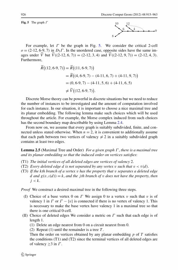
Fig. 5 The graph Γ
For example, let Γ be the graph in Fig. 5. We consider the critical 2-cello = (2-12,6-9,7) in D3Γ . In the unordered case, opposite sides have the same im-ages under V but V ((2-12,6,7)) = (2-12,3,4) and V ((2-12,9,7)) = (2-12,4,3).Furthermore,
R((12,6-9,7)
)= R((11,6-9,7)
)
= R((4,6-9,7) − (4-11,6,7) + (4-11,9,7)
)
= (0,6-9,7) − (4-11,5,6) + (4-11,6,5)
�= V((12,6-9,7)
).
Discrete Morse theory can be powerful in discrete situations but we need to reducethe number of instances to be investigated and the amount of computation involvedfor each instance. In our situation, it is important to choose a nice maximal tree andits planar embedding. The following lemma make such choices which will be usedthroughout the article. For example, the Morse complex induced from such choiceshas the second boundary map describable by using Lemma 2.4.
From now on, we assume that every graph is suitably subdivided, finite, and con-nected unless stated otherwise. When n = 2, it is convenient to additionally assumethat each path between two vertices of valency �= 2 in a suitably subdivided graphcontains at least two edges.
Lemma 2.5 (Maximal Tree and Order) For a given graph Γ , there is a maximal treeand its planar embedding so that the induced order on vertices satisfies:
(T1) The initial vertices of all deleted edges are vertices of valency 2.(T2) Every deleted edge d is not separated by any vertex v such that v < τ(d).(T3) If the kth branch of a vertex v has the property that v separates a deleted edge
d and g(v, ι(d)) = k, and the j th branch of v does not have the property, thenj < k.
Proof We construct a desired maximal tree in the following three steps.
(I) Choice of a base vertex 0 on Γ We assign 0 to a vertex v such that v is ofvalency 1 in Γ or Γ − {v} is connected if there is no vertex of valency 1. Thisis necessary to make the base vertex have valency 1 in a maximal tree so thatthere is one critical 0-cell.
(II) Choice of deleted edges We consider a metric on Γ such that each edge is oflength 1.(1) Delete an edge nearest from 0 on a circuit nearest from 0.(2) Repeat (1) until the remainder is a tree T .Then the order on vertices obtained by any planar embedding p of T satisfiesthe conditions (T1) and (T2) since the terminal vertices of all deleted edges areof valency ≥3 in Γ .
Discrete Comput Geom (2012) 48:915–963 927
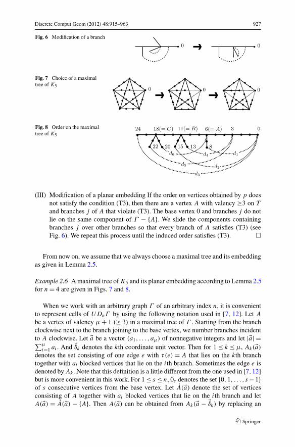
Fig. 6 Modification of a branch
Fig. 7 Choice of a maximaltree of K5
Fig. 8 Order on the maximaltree of K5
(III) Modification of a planar embedding If the order on vertices obtained by p doesnot satisfy the condition (T3), then there are a vertex A with valency ≥3 on T
and branches j of A that violate (T3). The base vertex 0 and branches j do notlie on the same component of Γ − {A}. We slide the components containingbranches j over other branches so that every branch of A satisfies (T3) (seeFig. 6). We repeat this process until the induced order satisfies (T3). �
From now on, we assume that we always choose a maximal tree and its embeddingas given in Lemma 2.5.
Example 2.6 A maximal tree of K5 and its planar embedding according to Lemma 2.5for n = 4 are given in Figs. 7 and 8.
When we work with an arbitrary graph Γ of an arbitrary index n, it is convenientto represent cells of UDnΓ by using the following notation used in [7, 12]. Let A
be a vertex of valency μ + 1 (≥ 3) in a maximal tree of Γ . Starting from the branchclockwise next to the branch joining to the base vertex, we number branches incidentto A clockwise. Let �a be a vector (a1, . . . , aμ) of nonnegative integers and let |�a| =∑μ
i=1 ai . And �δk denotes the kth coordinate unit vector. Then for 1 ≤ k ≤ μ, Ak(�a)
denotes the set consisting of one edge e with τ(e) = A that lies on the kth branchtogether with ai blocked vertices that lie on the ith branch. Sometimes the edge e isdenoted by Ak . Note that this definition is a little different from the one used in [7, 12]but is more convenient in this work. For 1 ≤ s ≤ n, 0s denotes the set {0,1, . . . , s −1}of s consecutive vertices from the base vertex. Let A(�a) denote the set of verticesconsisting of A together with ai blocked vertices that lie on the ith branch and letA(�a) = A(�a) − {A}. Then A(�a) can be obtained from Ak(�a − �δk) by replacing an
928 Discrete Comput Geom (2012) 48:915–963
edge e with ι(e). Every critical i-cell is represented by the following union:
A1k1
(�a1)∪ · · · ∪ A�k�
(�a�)∪ {d1, . . . , dq} ∪ {v1, . . . , vr} ∪ 0s ,
where A1, . . . ,A� are vertices of valency ≥3, and d1, . . . , dq are deleted edges, andv1, . . . , vr are blocked vertices blocked by deleted edges. Furthermore, since s isuniquely determined by s = n− (�+|�a1|+ · · ·+ |�a�|+q + r), we will omit 0s in thenotation. Let �a − 1 denote the vector obtained from �a by subtracting 1 from the firstpositive entry. Then �a − α denotes the vector obtained from �a by iterating the aboveoperation α times. Define p(�a) = i if ai is the first nonzero entry of �a. For 1 ≤ k ≤ μ,set (�a)k = (a1, . . . , ak−1,0, . . . ,0) and |�a|k = a1 + · · · + ak−1.
By condition (T1), there are no vertices blocked by the initial vertex of any deletededge. Let d(�a) denote the set consisting of a deleted edge d together with ai blockedvertices that lie on the ith branch of τ(d) for each i. Every critical 2-cell can berepresented by one of the following forms:
Ak(�a) ∪ B�(�b), Ak(�a) ∪ d(�b), d(�a) ∪ d ′(�b)
where A and B are vertices of valency ≥3 in T , d and d ′ are deleted edges. Condition(T2) implies that there is no pair of edges such that the terminal vertex of one edgeseparates the other edge and vice versa. So we need not handle this troublesome case.Condition (T3) will be used in Sect. 3.1.
The following notation is useful in describing images under the second boundarymap:
A(�a, �) = R
( |�a|∑
α=0
Ap(�a−α)
((�a − α) − �δp(�a−α) + �δ�
))
where A is a vertex of valency ≥3, �a is a vector defined at A, and 1 ≤ � ≤ μ. It isstraightforward to see that a sum of critical 1-cells represented by this notation hasthe following properties.
Proposition 2.7
(i) If am = bm for all m > �, then A(�a, �) = A(�b, �).(ii) If p(�a) > �, then A(�a, �) − A(�a − 1, �) = R(Ap(�a)(�a − �δp(�a) + �δ�)).
As mentioned above, there are three types of critical 2-cells. We will describe theimages of each of these three types under ∂ . Since an edge Ak is never separatedby any vertex, Lemma 2.5 implies ∂(Ak(�a) ∪ B�(�b)) = 0, which was first proved byFarley and Sabalka in [7]. So we consider the remaining two types. To help grasp theidea behind, examples are followed by general formulae.
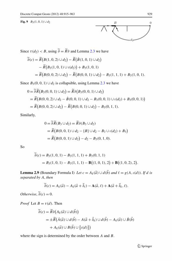
Example 2.8 Let Γ be K5 and a maximal tree and an order be given as in Exam-ple 2.6. We want to compute ∂(c) for the 2-cell c = B3(1,0,1) ∪ d2 in M2(UD4Γ )
(see Fig. 9).
Discrete Comput Geom (2012) 48:915–963 929
Fig. 9 B3(1,0,1) ∪ d2
Since τ(d2) < B , using ∂ = R∂ and Lemma 2.3 we have
∂(c) = R(B(1,0,2) ∪ d2
)− R(B(1,0,1) ∪ d2
)
− R(B3(1,0,1) ∪ ι(d2)
)+ B3(1,0,1)
= R(B(0,0,2) ∪ d2
)− R(B(0,0,1) ∪ d2
)− B3(1,1,1) + B3(1,0,1).
Since B3(0,0,1) ∪ d2 is collapsible, using Lemma 2.3 we have
0 = ∂R(B3(0,0,1) ∪ d2
)= R∂(B3(0,0,1) ∪ d2
)
= R(B(0,0,2) ∪ d2 − B(0,0,1) ∪ d2 − B3(0,0,1) ∪ ι(d2) + B3(0,0,1)
)
= R(B(0,0,2) ∪ d2
)− R(B(0,0,1) ∪ d2
)− B3(0,1,1).
Similarly,
0 = ∂R(B3 ∪ d2) = R∂(B3 ∪ d2)
= R(B(0,0,1) ∪ d2 − {B} ∪ d2 − B3 ∪ ι(d2) + B3
)
= R(B(0,0,1) ∪ d2
)− d2 − B3(0,1,0).
So
∂(c) = B3(1,0,1) − B3(1,1,1) + B3(0,1,1)
= B3(1,0,1) − B3(1,1,1) − B((1,0,1),2
)+ B((1,0,2),2
).
Lemma 2.9 (Boundary Formula I) Let c = Ak(�a) ∪ d(�b) and � = g(A, ι(d)). If d isseparated by A, then
∂(c) = Ak(�a) − Ak(�a + �δ�) − A(�a, �) + A(�a + �δk, �).
Otherwise, ∂(c) = 0.
Proof Let B = τ(d). Then
∂(c) = R∂(Ak(�a) ∪ d(�b)
)
= ±R(A(�a) ∪ d(�b) − A(�a + �δk) ∪ d(�b) − Ak(�a) ∪ B(�b)
+ Ak(�a) ∪ B(�b) ∪ {ι(d)})
where the sign is determined by the order between A and B .
930 Discrete Comput Geom (2012) 48:915–963
Fig. 10 d6(0,1) ∪ d4
Since Ak is not separated by any vertex, Lemma 2.4 implies R(Ak(�a) ∪ B(�b)) =R ◦ V (Ak(�a)∪ B(�b)) and R(Ak(�a)∪B(�b)∪{ι(d)}) = R ◦ V (Ak(�a)∪B(�b)∪{ι(d)}).
Assume that d is not separated by A. Then V (Ak(�a)∪ B(�b)) = V (Ak(�a)∪B(�b)∪{ι(d)}). So we only consider R(A(�a)∪d(�b)−A(�a + �δk)∪d(�b)). Let C be the uniquelargest vertex of valency ≥3 such that C < A. Since d is not separated by any vertexbetween C and A, Lemma 2.3 implies R(A(�a) ∪ d(�b)) = R(C((|�a| + 1)�δg(C,A)) ∪d(�b)) = R(A(�a + �δk) ∪ d(�b)). Thus ∂(c) = 0.
Assume that d is separated by A. By condition (T1) on our maximal tree, A > B
= τ(d) and so the negative sign is valid in the expression of ∂(c) above. Lemma 2.4implies R(Ak(�a) ∪ B(�b)) = Ak(�a) and R(Ak(�a) ∪ B(�b) ∪ {ι(d)}) = R ◦ V (Ak(�a +�δ�) ∪ B(�b)) = Ak(�a + �δ�). Let m = g(B,A). Since R(A(�a) ∪ d(�b)) = R(A(�a) ∪d(�b + �δm)), it is sufficient to prove the formula
R(A(�a) ∪ d(�b)
)= d(�b + |�a|�δm
)+ A(�a, �).
We use the induction on |�a|.
R(A(�a) ∪ d(�b)
)
= R(A(�a − 1) ∪ d(�b) + Ap(�a)(�a − �δp(�a)) ∪ B(�b) ∪ {ι(d)
})
− R(Ap(�a)(�a − �δp(�a)) ∪ B(�b)
)
= R(A(�a − 1) ∪ d(�b + �δm) + Ap(�a)(�a + �δ� − �δp(�a)) − Ap(�a)(�a − �δp(�a))
)
= d(�b + |�a|�δm
)+ A(�a − 1, �) + R(Ap(�a)(�a + �δ� − �δp(�a))
)
= d(�b + |�a|�δm
)+ A(�a, �).
Notice that Ap(�a)(�a − �δp(�a)) is collapsible. It is easy to verify the formula for|�a| = 1. �
Let d and d ′ be deleted edges such that τ(d) > τ(d ′), C = ι(d) ∧ ι(d ′),� = min{g(C, ι(d)), g(C, ι(d ′))} and k = max{g(C, ι(d)), g(C, ι(d ′))}. Then we de-fine
∧(d, d ′)= Ck(�δ�).
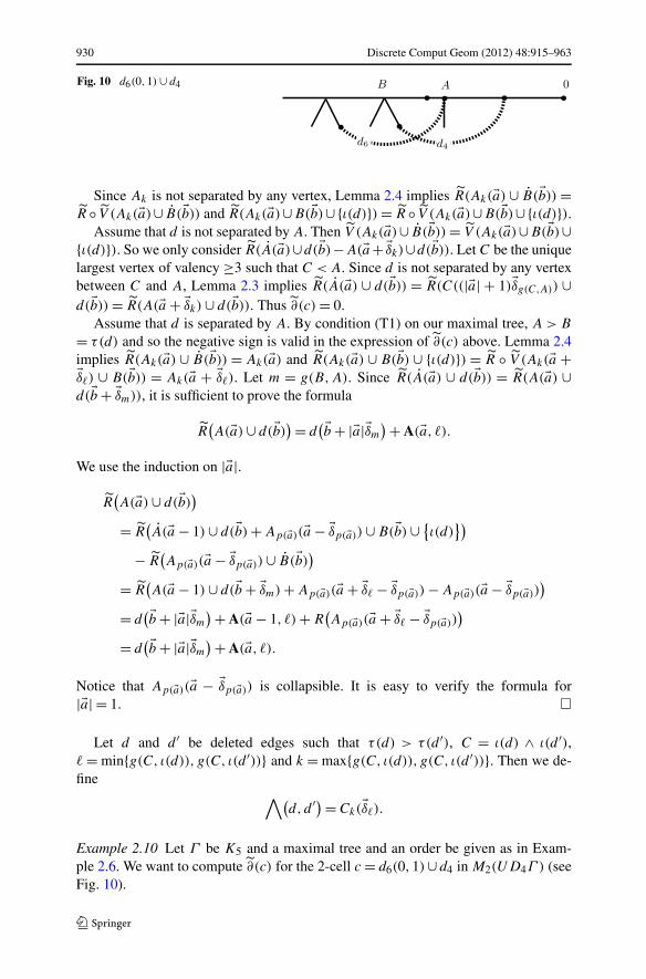
Example 2.10 Let Γ be K5 and a maximal tree and an order be given as in Exam-ple 2.6. We want to compute ∂(c) for the 2-cell c = d6(0,1) ∪ d4 in M2(UD4Γ ) (seeFig. 10).
Discrete Comput Geom (2012) 48:915–963 931
Since τ(d4) < τ(d6), using ∂ = R∂ and Lemma 2.3, we have
∂(c) = R(A(0,1) ∪ {ι(d6)
}∪ d4)− R
(A(0,1) ∪ d4
)
− R(d6(0,1) ∪ ι(d4)
)+ R(d6(0,1) ∪ τ(d4)
)
= R(B(0,0,1) ∪ d4(1)
)− d4(2) − d6(0,2) + d6(0,1).
Since B3 ∪ d4(1) is collapsible, using Lemma 2.3 we have
0 = ∂R(B3 ∪ d4(1)
)= R∂(B3 ∪ d4(1)
)
= R(B(0,0,1) ∪ d4(1) − {B} ∪ d4(1) − B3 ∪ ι(d4) + B3
)
= R(B(0,0,1) ∪ d4(1)
)− d4(2) − B3(1,0,0).
So
∂(c) = d6(0,1) − d6(0,2) + {d4(2) + B3(1,0,0)}− d4(2)
= d6(0,1) − d6(0,2) +∧
(d6, d4).
Lemma 2.11 (Boundary Formula II) Let c = d(�a) ∪ d ′(�b) such that τ(d) > τ(d ′)and let A = τ(d), k = g(A, ι(d)), and � = g(A, ι(d ′)). If d ′ is separated by A, then
∂(c) = d(�a) − d(�a + �δk) − A(�a, �) + A(�a + �δk, �) + ε ∧ (d, d ′)
where ε = 0 for k �= �, ε = −1 for k = � and ι(d) < ι(d ′), and ε = 1 for k = � andι(d ′) < ι(d). Otherwise, ∂(c) = 0.
Proof Let B = τ(d ′). Then A = τ(d) > B . So
∂(c) = R(A(�a) ∪ d ′(�b) ∪ {ι(d)
}− A(�a) ∪ d ′(�b) − d(�a) ∪ B(�b) ∪ {ι(d ′)}
+ d(�a) ∪ B(�b)).
Note that d is not separated by B . Assume d ′ is not separated by A. By Lemma 2.4,R(A(�a) ∪ d ′(�b) ∪ {ι(d)}) = R(A(�a) ∪ d ′(�b)), R(d(�a) ∪ B(�b) ∪ {ι(d ′)}) = R(d(�a) ∪B(�b)) and so ∂(c) = 0.
Now assume that d ′ is separated by A. If k �= �, then d ′ (and d , respectively) is notseparated by any vertex other than A on the path between A and ι(d) (and ι(d ′)). Sowe see that R(A(�a) ∪ d ′(�b) ∪ {ι(d)}) = R(A(�a + �δk) ∪ d ′(�b)) and R(d(�a) ∪ B(�b) ∪{ι(d ′)}) = R(d(�a + �δ�) ∪ B(�b)).
Assume k = �. Let C = ι(d) ∧ ι(d ′), m = g(C, ι(d ′)) and p = g(C, ι(d)). ThenA < C. If ι(d) < ι(d ′), then p < m and so Lemma 2.4 implies
R(A(�a) ∪ d ′(�b) ∪ {ι(d)
})= R(A(�a + �δk) ∪ d ′(�b)
).
And we have
932 Discrete Comput Geom (2012) 48:915–963
R(d(�a) ∪ B(�b) ∪ {ι(d ′)})
= R(d(�a) ∪ B(�b) ∪ {C} + A(�a) ∪ B(�b) ∪ Cm(δm) ∪ {ι(d)
})
− R(A(�a) ∪ B(�b) ∪ Cm(�δm)
)
= R(d(�a + �δ�) ∪ B(�b)
)+ R(A(�a) ∪ B(�b) ∪
∧(d, d ′))
= R(d(�a + �δ�) ∪ B(�b)
)+∧(
d, d ′).
Finally if ι(d ′) < ι(d), then m < p and so Lemma 2.4 implies
R(A(�a) ∪ d ′(�b) ∪ {ι(d)
})
= R(A(�a) ∪ d ′(�b) ∪ {C} − A(�a) ∪ B(�b) ∪ Cp(δp) ∪ {ι(d ′)})
+ R(A(�a) ∪ B(�b) ∪ Cp(�δp)
)
= R(A(�a + �δk) ∪ d ′(�b)
)+ R(A(�a) ∪ B(�b) ∧ (d, d ′))
= R(A(�a + �δk) ∪ d ′(�b)
)+∧(
d, d ′).
And we have
R(d(�a) ∪ B(�b) ∪ {ι(d ′)})= R
(d(�a + �δ�) ∪ B(�b)
).
The remaining part can be proved by the same argument as in the proof ofLemma 2.9. �
To prove that for planar graphs the first homologies of graph braid groups aretorsion-free, we need an additional requirement. So we modify Lemma 2.5 for planargraphs as follows.
Lemma 2.12 (Maximal Tree and Order for Planar Graph) For a given planar graphΓ , there is a maximal tree and its planar embedding so that the induced order onvertices satisfies (T1), (T2), and (T3) in Lemma 2.5, and additionally
(T4) If τ(d ′) < τ(d) and g(τ(d), ι(d)) = g(τ(d), ι(d ′)) then ι(d) < ι(d ′).
Proof Since Γ is suitably subdivided, each path between two vertices of valency �= 2passes through at least 2 edges.
(I) Choices of a base vertex 0 and a planar embedding We assign 0 to a vertex v
such that v is of valency 1 in Γ or Γ − {v} is connected if there is no vertex ofvalency 1. Choose a planar embedding of Γ such that the base vertex 0 lies inthe outmost region. Let T = Γ . Go to Step II.
(II) Choice of deleted edges Take a regular neighborhood R of T . As traveling theoutmost component of ∂R clockwise from the base vertex until either comingback to 0 or meeting an edge that is on a circuit. If the former is the case, we aredone. If the latter is the case, delete the edge and let T be the rest. Repeat Step II.
Discrete Comput Geom (2012) 48:915–963 933
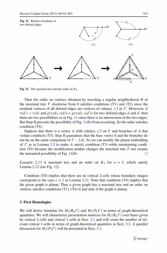
Fig. 11 Relative locations oftwo deleted edges
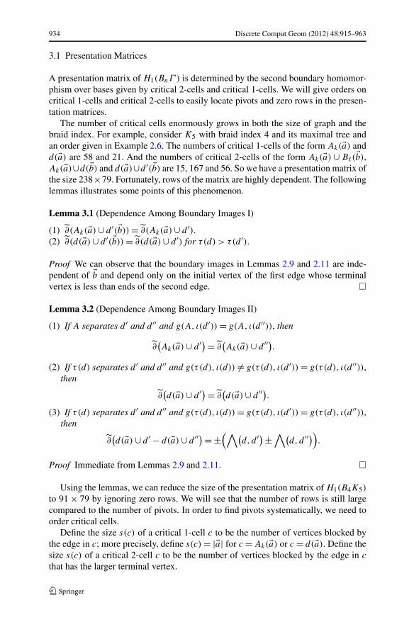
Fig. 12 The maximal tree and the order on K4
Then the order on vertices obtained by traveling a regular neighborhood R ofthe maximal tree T clockwise from 0 satisfies conditions (T1) and (T2) since theterminal vertices of all deleted edges are vertices of valency ≥3 in Γ . Moreover, ifτ(d ′) < τ(d) and g(τ(d), ι(d)) = g(τ(d), ι(d ′)) for two deleted edges d and d ′ thenthere are two possibilities as in Fig. 11 since there is no intersection of the two edges.But Step II prevents the possibility of Fig. 11(b) from occurring. So the order satisfiescondition (T4).
Suppose that there is a vertex A with valency ≥3 on T and branches of A thatviolate condition (T3). Step II guarantees that the base vertex 0 and the branches donot lie on the same component of Γ − {A}. So we can modify the planar embeddingof Γ as in Lemma 2.5 to make A satisfy condition (T3) while maintaining condi-tion (T4) because the modification neither changes the maximal tree T nor createsthe unwanted possibility of Fig. 11(b). �
Example 2.13 A maximal tree and an order on K4 for n = 3, which satisfyLemma 2.12 (see Fig. 12).
Condition (T4) implies that there are no critical 2-cells whose boundary imagescorrespond to the case ε = 1 in Lemma 2.11. Note that condition (T4) implies thatthe given graph is planar. Thus a given graph has a maximal tree and an order onvertices satisfies conditions (T1)–(T4) if and only if the graph is planar.
3 First Homologies
We will derive formulae for H1(BnΓ ) and H1(P2Γ ) in terms of graph-theoreticalquantities. We will characterize presentation matrices for H1(BnΓ ) over bases givenby critical 2-cells and critical 1-cells in Sect. 3.1 and will count the number of rel-evant critical 1-cells in terms of graph-theoretical quantities in Sect. 3.2. A paralleldiscussion for H1(P2Γ ) will be presented in Sect. 3.3.
934 Discrete Comput Geom (2012) 48:915–963
3.1 Presentation Matrices
A presentation matrix of H1(BnΓ ) is determined by the second boundary homomor-phism over bases given by critical 2-cells and critical 1-cells. We will give orders oncritical 1-cells and critical 2-cells to easily locate pivots and zero rows in the presen-tation matrices.
The number of critical cells enormously grows in both the size of graph and thebraid index. For example, consider K5 with braid index 4 and its maximal tree andan order given in Example 2.6. The numbers of critical 1-cells of the form Ak(�a) andd(�a) are 58 and 21. And the numbers of critical 2-cells of the form Ak(�a) ∪ B�(�b),Ak(�a)∪d(�b) and d(�a)∪d ′(�b) are 15, 167 and 56. So we have a presentation matrix ofthe size 238×79. Fortunately, rows of the matrix are highly dependent. The followinglemmas illustrates some points of this phenomenon.
Lemma 3.1 (Dependence Among Boundary Images I)
(1) ∂(Ak(�a) ∪ d ′(�b)) = ∂(Ak(�a) ∪ d ′).(2) ∂(d(�a) ∪ d ′(�b)) = ∂(d(�a) ∪ d ′) for τ(d) > τ(d ′).
Proof We can observe that the boundary images in Lemmas 2.9 and 2.11 are inde-pendent of �b and depend only on the initial vertex of the first edge whose terminalvertex is less than ends of the second edge. �
Lemma 3.2 (Dependence Among Boundary Images II)
(1) If A separates d ′ and d ′′ and g(A, ι(d ′)) = g(A, ι(d ′′)), then
∂(Ak(�a) ∪ d ′)= ∂
(Ak(�a) ∪ d ′′).
(2) If τ(d) separates d ′ and d ′′ and g(τ(d), ι(d)) �= g(τ(d), ι(d ′)) = g(τ(d), ι(d ′′)),then
∂(d(�a) ∪ d ′)= ∂
(d(�a) ∪ d ′′).
(3) If τ(d) separates d ′ and d ′′ and g(τ(d), ι(d)) = g(τ(d), ι(d ′)) = g(τ(d), ι(d ′′)),then
∂(d(�a) ∪ d ′ − d(�a) ∪ d ′′)= ±
(∧(d, d ′)±
∧(d, d ′′)).
Proof Immediate from Lemmas 2.9 and 2.11. �
Using the lemmas, we can reduce the size of the presentation matrix of H1(B4K5)
to 91 × 79 by ignoring zero rows. We will see that the number of rows is still largecompared to the number of pivots. In order to find pivots systematically, we need toorder critical cells.
Define the size s(c) of a critical 1-cell c to be the number of vertices blocked bythe edge in c; more precisely, define s(c) = |�a| for c = Ak(�a) or c = d(�a). Define thesize s(c) of a critical 2-cell c to be the number of vertices blocked by the edge in c
that has the larger terminal vertex.
Discrete Comput Geom (2012) 48:915–963 935
We assume that a set of m-tuples is always lexicographically ordered in the discus-sion below. For edges e, e′, Declare e > e′ if e is a deleted edge and e′ is an edge onT or if both are either deleted edges or edges on T and (τ (e), ι(e)) > (τ(e′), ι(e′)).The set of critical 1-cells c is linearly ordered by triples (s(c), e, �a) where c is givenby either Ak(�a) or d(�a). The following lemma motivates this order.
Lemma 3.3 (Leading Coefficient) Let c be a critical 2-cell containing two edges e
and e′ such that τ(e) > τ(e′). Assume that �a represent vertices blocked by τ(e) in c. If∂(c) �= 0 then the largest summand in ∂(c) has the triple (s(c)+1, e, �a+�δg(τ(e),ι(e′))).Furthermore, if e is a deleted edge d , then the largest summand is −d(�a +�δg(τ(e),ι(e′))) and if e is on T , then the largest summand is −Ak(�a + �δg(τ(e),ι(e′)))where A = τ(e) and k = g(A, ι(e)).
Proof By Lemmas 2.9 and 2.11 we see that ∂(c) is determined by e, �a and τ(e′).Using the order on critical 1-cells, it is easy to verify the lemma. �
In the view of this lemma, it is natural to order critical 2-cells as follows. For acritical 2-cell c, let e and e′ denote edges in c such that τ(e) > τ(e′) and �a and �a′represent vertices blocked by e and e′, respectively. The set of critical 2-cells c islinearly ordered by 6-tuples
(s(c), e, �a + �δg(τ(e),ι(e′)), g
(τ(e), ι
(e′)), e′, �a′).
Then the first three terms determine the largest summand in ∂(c). The fourth termhelps to find the boundary image of c other than a summand of the form
∧(d, d ′)
and the last two terms are added to make the order linear.Lemma 3.3 implies that the second boundary homomorphism ∂ is represented
by a block-upper-triangular matrix over bases of critical 2-cells and critical 1-cellsordered reversely. In fact, the presentation matrix is divided into blocks by s(c) andeach block is further divided into smaller blocks by the value e of 6-tuples. The firstcolumn of each diagonal block is a vector of −1. The −1 entry at the lower left cornerof each diagonal block will be called a pivot and a critical 2-cell corresponding to apivotal row is said to be pivotal. In other word, a pivotal 2-cell is the smallest oneamong all critical 2-cells that have the same (up to sign) largest summand in theirboundary images. The following lemma says that non-pivotal rows turn into a zerorow with few exceptions under row operations.
Lemma 3.4 (Non-pivotal Rows) Let c be a non-pivotal critical 2-cell such that∂(c) �= 0. If s(c) ≥ 1, then the row corresponding to c is a linear combination ofrows below. If s(c) = 0, then the row corresponding to c is either a linear combina-tion of rows below or made into a row consisting of only two nonzero entries that are±1 by row operations.
Proof Assume e′ is a deleted d ′ separated by τ(e) since ∂(c) = 0 otherwise. We mayalso assume that c is the smallest among all critical 2-cells whose boundary imagesequal to ∂(c). Then by Lemmas 3.1 and 3.2, the 6-tuple for c is given by
(s(c), e, �a + �δg(τ(e),ι(d ′)), g
(τ(e), ι
(d ′)), d ′,0
)
936 Discrete Comput Geom (2012) 48:915–963
so that there is no smaller deleted edge d ′′ separated by τ(e) satisfying g(τ(e),
ι(d ′)) = g(τ(e), ι(d ′′)). Set k = g(τ(e), ι(e)) and � = g(τ(e), ι(d ′)).There are three possibilities: (I) s(c) ≥ 1 and c = d(�a) ∪ d ′, (II) s(c) ≥ 1 and
c = Ak(�a) ∪ d ′, and (III) s(c) = 0 and c = d ∪ d ′.
(I) Assume s(c) ≥ 1 and c = d(�a) ∪ d ′ Set A = τ(d). We consider the followingtwo cases separately:(a) There is a deleted edge d ′′ separated by A such that am �= 0 and m < � for
m = g(A, ι(d ′′));(b) There is no such a deleted edge.For case (a), we consider the following boundary image of a linear combination:
∂(d(�a) ∪ d ′ − d(�a + �δ� − �δm) ∪ d ′′ − d(�a − �δm) ∪ d ′ + d(�a − �δm) ∪ d ′′)
= A(�a + �δ� − �δm,m) − A(�a − �δm,m)
− {A(�a + �δ� − �δm + �δk,m) − A(�a − �δm + �δk,m)}.
The three terms other than c on the left side of the equation are critical 2-cellsless than c. So it is sufficient to show that the right side, which will be denotedby R, is a linear combination of boundary images of critical 2-cells less than c.The sum R depends on the order among k, � and m. If m ≥ k then A(�a + �δ� −�δm,m) = A(�a + �δ� − �δm + �δk,m) and A(�a − �δm,m) = A(�a − �δm + �δk,m) byProposition 2.7 and so R = 0.
Since m < �, Proposition 2.7 and Lemma 2.9 imply that for any �x,
∂ ◦ R
( |�x|�∑
α=0
Ap(�x−α)
((�x − α) − �δp(�x−α) + �δm
)∪ d ′)
= A(�x,m) − A(�x + �δ�,m) + A�
((�x − |�x|�)+ �δm
).
To shorten formulae, let �b = �a − �δm + �δk and �c = �a − �δm. If m < k. then
R = ∂ ◦ R
( |�b|�∑
α=0
Ap(�b−α)
((�b − α) − �δ
p(�b−α)+ �δm
)∪ d ′)
− ∂ ◦ R
( |�c|�∑
α=0
Ap(�c−α)
((�b − α) − �δ
p(�b−α)+ �δm
)∪ d ′)
− A�
((�b − |�b|�)+ �δm
)+ A�
((�c − |�c|�)+ �δm
).
If m < k < �, �b − |�b|� = �c − |�c|� by Lemma 2.9. If m < � ≤ k,
∂(A�
((�c − |�c|�)+ �δm
)∪ d ′′′)= A�
((�b − |�b|�)+ �δm
)− A�
((�c − |�c|�)+ �δm
)
since there is a deleted edge d ′′′ separated by A such that k = g(A, ι(d ′′′)) by(T3) of Lemma 2.5.
Discrete Comput Geom (2012) 48:915–963 937
In case (b), by the assumption there is no deleted edge d ′′ separated by τ(d)
such that g(A, ι(d ′′)) = m < � and xm �= 0 for �x = �a + �δ� and so there is nocritical 2-cell with the 6-tuple (s(c), d, �x,m,d ′′,0) such that m < � and A sep-arates d ′′. If k �= �, c would be pivotal by the assumption on c. So k = �. ByLemma 3.2(3), ∂(d(�a)∪ d ′ − d(�a)∪ d ′′′) = ∂(d ∪ d ′ − d ∪ d ′′′) where d ′′′ is thesmallest deleted edge such that A separates d ′′′ and g(A, ι(d ′′′)) = �. Note that|�a| ≥ 1 since s(c) ≥ 1. And d ′′′ < d ′ since c is pivotal. Thus we have a desiredlinear combination.
(II) Assume s(c) ≥ 1 and c = Ak(�a) ∪ d ′ Consider the following cases separately:(a) There is a deleted edge d ′′ separated by A such that g(A, ι(d ′′)) = m < �
and one of the following conditions holds:(i) am ≥ 1 if k ≤ m,
(ii) am ≥ 1 and |�a|k ≥ 2 if m < k ≤ �,(iii) am ≥ 1 and |�a|k ≥ 2 if m < � < k, and(iv) am ≥ 1 and |�a|k = 1 if m < � < k;
(b) There is no such a deleted edge.For cases (a)(i)–(iii), we consider the following boundary image of the linearcombination:
∂(Ak(�a) ∪ d ′ − Ak(�a + �δ� − �δm) ∪ d ′′ − Ak(�a − �δm) ∪ d ′ + Ak(�a − �δm) ∪ d ′′)
= A(�a + �δ� − �δm,m) − A(�a − �δm,m)
− {A(�a + �δ� − �δm + �δk,m) − A(�a − �δm + �δk,m)}.
The three terms other than c on the left side of the equation are critical 2-cellsless than c. Then it is sufficient to show that the right side is a linear combinationof boundary images of critical 2-cells less than c. We omit the proof since it issimilar to case (I)(a).
For case (a)(iv), we consider the following boundary image of the linearcombination:
∂(Ak(�a) ∪ d ′ − Ak(�a + �δ� − �δm) ∪ d ′′ − A�(�a + �δ� − �δk) ∪ d ′′′)= 0
where d ′′′ is a deleted edge separated by A and g(A, ι(d ′′′)) = k. Note that theexistence of d ′′′ is guaranteed by condition (T3) of Lemma 2.5.
We will show that case (b) does not happen. Suppose that there is nodeleted edge d ′′ separated by A such that g(A, ι(d ′′)) = m < � and Ak(�x − �δm)
is critical for �x = �a + �δ�. So there is no critical 2-cell with the 6-tuple(s(c),Ak(�δk), �x,m,d ′′,0) such that m < � and A separates d ′′. Then c wouldbe pivotal since d ′ is the smallest among deleted edges d ′′ separated by A suchthat g(A, ι(d ′′)) = �.
(III) Assume s(c) = 0 and c = d ∪ d ′ Let k = g(τ(d), ι(d)). Since c is non-pivotal,k = �. By Lemma 3.2(3), ∂(d ∪ d ′ − d ∪ d ′′) = ±(
∧(d, d ′) ±∧(d, d ′′)) where
d ′′ is the smallest deleted edge separated by A such that g(A, ι(d ′′)) = �. Notethat if d ′ = d ′′ then c would be pivotal. This completes the proof. �
We are ready to see the main theorem of this section.
938 Discrete Comput Geom (2012) 48:915–963
Theorem 3.5 Let M be a presentation matrix of H1(BnΓ ) represented by ∂ overbases of critical 2-cells and 1-cells ordered reversely. Up to row operations, eachrow of M satisfies one of the following:
(1) it consists of all zeros;(2) there is a ±1 entry that is the only nonzero entry in the column it belongs to;(3) there are only two nonzero entries which are ±1.
If Γ is planar then two nonzero entries in (3) have opposite signs. Furthermore, thenumber of rows satisfying (3) does not depend on braid indices.
Proof This theorem is merely a restatement of Lemma 3.4 via row operations. A piv-otal row corresponding to a pivotal 2-cell satisfies (2). A row of the type (3) is pro-duced from the relation ∂(d ∪d ′′ −d ∪d ′) = ±(
∧(d, d ′′)±∧(d, d ′)) in the last part
of the proof of the previous lemma. Note that neither∧
(d, d ′) nor∧
(d, d ′′) corre-spond to a pivotal column due to Lemma 3.3 and the order among critical 1-cells.
Obviously the number of these relations does not depend on braid indices. If Γ
is planar, the relation becomes ∂(d ∪ d ′′ − d ∪ d ′) = ±(∧
(d, d ′′) −∧(d, d ′)) byLemmas 2.11 and 2.12. Therefore two nonzero entries in (3) have opposite signs. �
Further row operations among rows of the type (3) in the theorem may producenew pivots ±2 but if two nonzero entries have opposite signs, all of new pivots are±1 and so we have the following corollary.
Corollary 3.6 If H1(BnΓ ) has a torsion, it is a 2-torsion and the number of2-torsions does not depend on braid indices. For a planar graph Γ , H1(BnΓ ) istorsion-free.
We classify critical 1-cells according to Theorem 3.5. A critical 1-cell is said to be:
(i) pivotal if it corresponds to pivotal columns, which is related to (2);(ii) separating if it corresponds to columns of nonzero entries of (3);
(iii) free otherwise.
Clearly, a pivotal 1-cell has no contribution to H1(BnΓ ) and a free 1-cell con-tributes a free summand to H1(BnΓ ). To complete the computation of H1(BnΓ ), itis enough to consider the submatrix obtained by deleting pivotal rows and zero rowsand deleting pivotal columns and columns of free 1-cells. This submatrix will be re-ferred as an undetermined block for H1(BnΓ ) and will be studied in Sect. 3.2. Rowsof an undetermined block are of the type (3) and columns correspond to separating1-cells. It will be useful later to have a geometric characterization of pivotal 1-cells.
Lemma 3.7 (Pivotal 1-Cell) A critical 1-cell c is pivotal if and only if c is eitherAk(�a) or d(�a) such that there is a deleted edge d ′ separated by A or τ(d) and am ≥ 1for m = g(A, ι(d ′)), and in addition s(c) ≥ 2 when c = Ak(�a).
Proof By the definition of pivotal 1-cell and Lemma 3.3, c is a pivotal 1-cell iff thereis a critical 2-cell whose boundary image has the largest summand c iff s(c) ≥ 2 for
Discrete Comput Geom (2012) 48:915–963 939
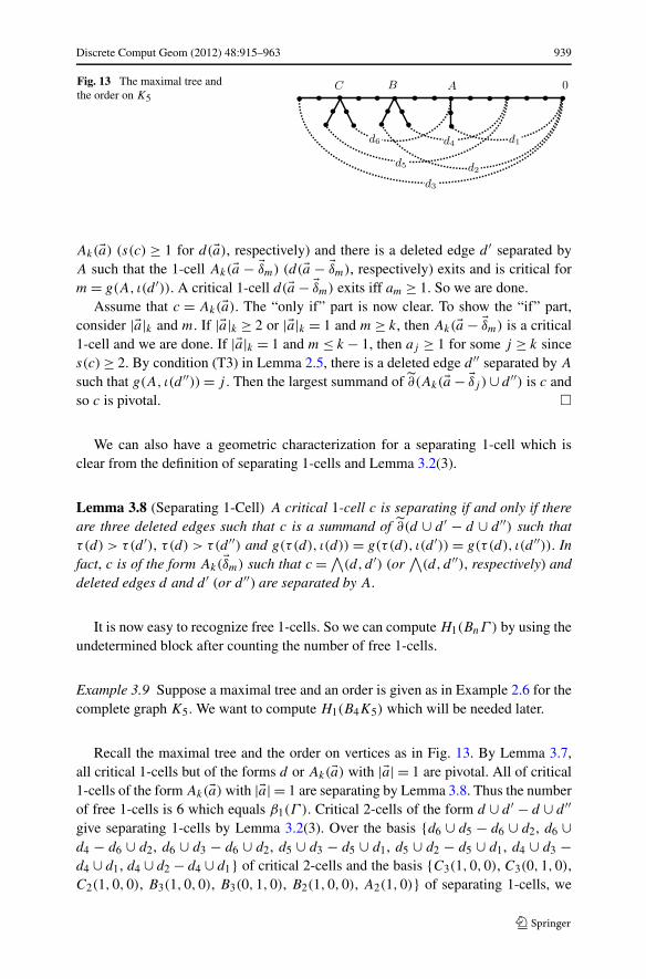
Fig. 13 The maximal tree andthe order on K5
Ak(�a) (s(c) ≥ 1 for d(�a), respectively) and there is a deleted edge d ′ separated byA such that the 1-cell Ak(�a − �δm) (d(�a − �δm), respectively) exits and is critical form = g(A, ι(d ′)). A critical 1-cell d(�a − �δm) exits iff am ≥ 1. So we are done.
Assume that c = Ak(�a). The “only if” part is now clear. To show the “if” part,consider |�a|k and m. If |�a|k ≥ 2 or |�a|k = 1 and m ≥ k, then Ak(�a − �δm) is a critical1-cell and we are done. If |�a|k = 1 and m ≤ k − 1, then aj ≥ 1 for some j ≥ k sinces(c) ≥ 2. By condition (T3) in Lemma 2.5, there is a deleted edge d ′′ separated by A
such that g(A, ι(d ′′)) = j . Then the largest summand of ∂(Ak(�a − �δj ) ∪ d ′′) is c andso c is pivotal. �
We can also have a geometric characterization for a separating 1-cell which isclear from the definition of separating 1-cells and Lemma 3.2(3).
Lemma 3.8 (Separating 1-Cell) A critical 1-cell c is separating if and only if thereare three deleted edges such that c is a summand of ∂(d ∪ d ′ − d ∪ d ′′) such thatτ(d) > τ(d ′), τ(d) > τ(d ′′) and g(τ(d), ι(d)) = g(τ(d), ι(d ′)) = g(τ(d), ι(d ′′)). Infact, c is of the form Ak(�δm) such that c =∧(d, d ′) (or
∧(d, d ′′), respectively) and
deleted edges d and d ′ (or d ′′) are separated by A.
It is now easy to recognize free 1-cells. So we can compute H1(BnΓ ) by using theundetermined block after counting the number of free 1-cells.
Example 3.9 Suppose a maximal tree and an order is given as in Example 2.6 for thecomplete graph K5. We want to compute H1(B4K5) which will be needed later.
Recall the maximal tree and the order on vertices as in Fig. 13. By Lemma 3.7,all critical 1-cells but of the forms d or Ak(�a) with |�a| = 1 are pivotal. All of critical1-cells of the form Ak(�a) with |�a| = 1 are separating by Lemma 3.8. Thus the numberof free 1-cells is 6 which equals β1(Γ ). Critical 2-cells of the form d ∪ d ′ − d ∪ d ′′give separating 1-cells by Lemma 3.2(3). Over the basis {d6 ∪ d5 − d6 ∪ d2, d6 ∪d4 − d6 ∪ d2, d6 ∪ d3 − d6 ∪ d2, d5 ∪ d3 − d5 ∪ d1, d5 ∪ d2 − d5 ∪ d1, d4 ∪ d3 −d4 ∪ d1, d4 ∪ d2 − d4 ∪ d1} of critical 2-cells and the basis {C3(1,0,0), C3(0,1,0),C2(1,0,0), B3(1,0,0), B3(0,1,0), B2(1,0,0), A2(1,0)} of separating 1-cells, we
940 Discrete Comput Geom (2012) 48:915–963
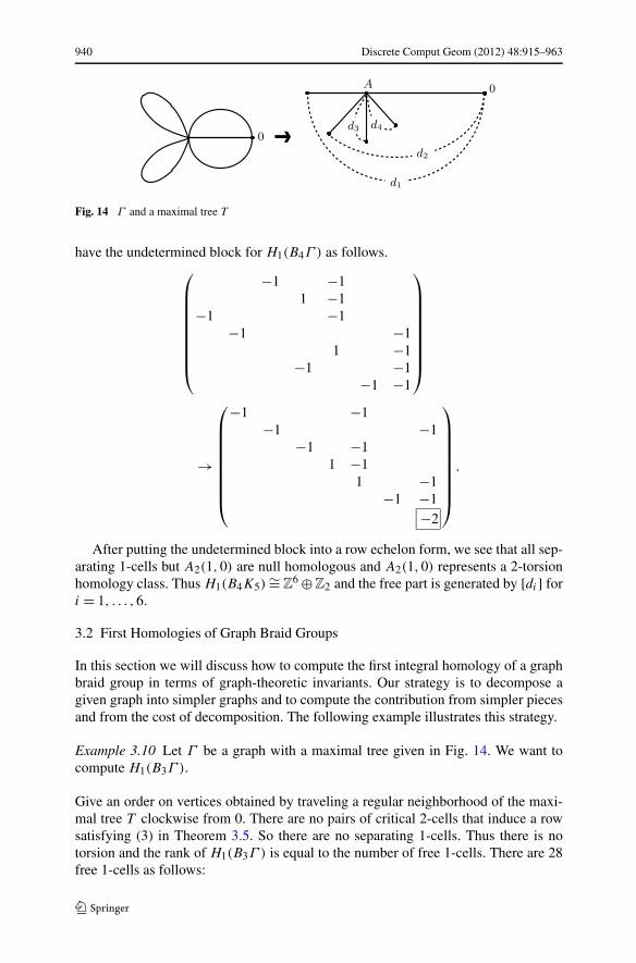
Fig. 14 Γ and a maximal tree T
have the undetermined block for H1(B4Γ ) as follows.⎛
⎜⎜⎜⎜⎜⎜⎜⎜⎝
−1 −11 −1
−1 −1−1 −1
1 −1−1 −1
−1 −1
⎞
⎟⎟⎟⎟⎟⎟⎟⎟⎠
→
⎛
⎜⎜⎜⎜⎜⎜⎜⎜⎝
−1 −1−1 −1
−1 −11 −1
1 −1−1 −1
−2
⎞
⎟⎟⎟⎟⎟⎟⎟⎟⎠
.
After putting the undetermined block into a row echelon form, we see that all sep-arating 1-cells but A2(1,0) are null homologous and A2(1,0) represents a 2-torsionhomology class. Thus H1(B4K5) ∼= Z
6 ⊕Z2 and the free part is generated by [di] fori = 1, . . . ,6.
3.2 First Homologies of Graph Braid Groups
In this section we will discuss how to compute the first integral homology of a graphbraid group in terms of graph-theoretic invariants. Our strategy is to decompose agiven graph into simpler graphs and to compute the contribution from simpler piecesand from the cost of decomposition. The following example illustrates this strategy.
Example 3.10 Let Γ be a graph with a maximal tree given in Fig. 14. We want tocompute H1(B3Γ ).
Give an order on vertices obtained by traveling a regular neighborhood of the maxi-mal tree T clockwise from 0. There are no pairs of critical 2-cells that induce a rowsatisfying (3) in Theorem 3.5. So there are no separating 1-cells. Thus there is notorsion and the rank of H1(B3Γ ) is equal to the number of free 1-cells. There are 28free 1-cells as follows:
Discrete Comput Geom (2012) 48:915–963 941
di for i = 1,2,3,4; di(�a) for i = 1,2 and �a = (1,0,0,0), (0,1,0,0), (2,0,0,0),
(1,1,0,0), (0,2,0,0); A2(�a) for �a = (1,0,0,0), (2,0,0,0), (1,1,0,0); A3(�a)
for �a = (1,0,0,0), (0,1,0,0), (2,0,0,0), (1,1,0,0), (0,2,0,0); and A4(�a) for�a = (1,0,0,0), (0,1,0,0), (0,0,1,0), (2,0,0,0), (1,1,0,0), (0,2,0,0).
Consequently, H1(B3Γ ) ∼= Z28.
The vertex A decomposes Γ into two circles and one Θ-shape graph that areall subgraphs of the original. The first homologies of two circles are generated byd4(2,0,0,0) and d3(0,2,0,0). And the first homology of Θ-shape graph is generatedby d1, d2 and A4(0,0,1,0). The remaining free 1-cells lie over at least two distinctcomponents and they are the cost of decomposition. So the first homology of Γ canalso be decomposed as
H1(B3Γ ) = ⟨d4(2,0,0,0)⟩⊕ ⟨d3(0,2,0,0)
⟩⊕ ⟨d1, d2,A4(0,0,1,0)⟩⊕ Z
23.
In order to formalize this idea, we need some notions and facts from graph theory.A cut of a connected graph is a set of vertices whose removal separates at least apair of vertices. A graph is k-vertex-connected if the size of a smallest cut is ≥k.If a graph has no cut (for example, complete graphs) and the number m of verticesis ≥2, then the graph is defined to be (m − 1)-vertex-connected. The graph of onevertex is defined to be 1-vertex-connected. The “2-vertex-connected” and “3-vertex-connected” will be referred to as biconnected and triconnected. Let C be a cut of Γ .A C-component is the closure of a connected component of Γ − C in Γ viewed astopological spaces. So a C-component is a subgraph of Γ .
Recall that we are assuming that every graph is suitably subdivided, finite, andconnected. A suitably subdivided graph is always simple, i.e has neither multipleedges nor loops, and moreover it has no edge between vertices of valency ≥3. A cutis called a k-cut if it contains k vertices. The set of 1-cuts of a graph Γ is well-definedand we can decompose Γ into components that are either biconnected or the completegraph K2 by iteratively taking C-components for all 1-cuts C. This decompositionis unique. The topological types of biconnected components of a given graph donot depend on subdivision. In fact, a subdivision merely affects the number of K2components.
Let C be a 2-cut {x, y} of a biconnected graph Γ . We find it convenient to modifyeach C-component by adding an extra edge between x and y. We refer to this modi-fied C-component as a marked C-component. If a marked C-component has a 2-cutC′, we take all marked C′-components of the marked C-component. By iterating thisprocedure, we can decompose a biconnected graph into components that are eithertriconnected or the complete graph K3. This decomposition is unique for a bicon-nected suitably subdivided graph (for example, see [5]) and will be called a markeddecomposition. The topological types of triconnected components of a given graphdo not depend on subdivision. In fact, a subdivision merely affects the number of K3components.
A graph is said to have topologically a certain property if it has the property afterignoring vertices of valency 2. We assume that each component in the above twodecompositions is always suitably subdivided by subdividing it if necessary. Thentriconnected components in the above decompositions are topologically triconnected.Note that a subdivision of a biconnected graph is again biconnected.
942 Discrete Comput Geom (2012) 48:915–963
Lemma 3.11 (Decomposition of Connected Graph) Let x be a 1-cut in a graph Γ .Then
H1(BnΓ ) ∼=(
μ⊕
i=1
H1(BnΓx,i)
)
⊕ ZN(n,Γ,x)
where Γx,i are x-components of Γ ,
N(n,Γ,x) =(
n + μ − 2n − 1
)× (ν − 2) −
(n + μ − 2
n
)− (ν − μ − 1),
μ is the number of x-components of Γ , and ν is the valency of x in Γ .
Proof Assume that Γ has a maximal tree T and an order on vertices as Lemma 2.5.Except the x-component containing the base vertex 0, each x-component Γx,i hasnew base point x and we maintain the numbering on vertices. Then x is the small-est vertex on each x-component not containing the original base vertex 0. UnlessA = x, every critical 1-cell of the type Ak(�a) can be thought of as a critical 1-cell inone of x-components by regarding vertices blocked by 0 as vertices blocked by x.Similarly, unless ι(d) = x or τ(d) = x, a deleted edge d does not join distinctx-components and so a critical 1-cell of the type d(�a) can be regarded as a criti-cal 1-cell in one of x-components. Therefore a critical 1-cell in UDnΓ that belongsto none of x-components must contain an edge incident to x.
We first claim that the undetermined block for H1(BnΓ ) is a block sum of theundetermined blocks for H1(BnΓx,i)’s. A row of an undetermined block is obtainedby the boundary image of a critical 2-cell of the form d ∪ d ′ (see Lemma 3.8). Iftwo deleted edges d and d ′ are in distinct x-component, the boundary image is trivialsince the terminal vertex of one edge cannot separate the other. Thus both d and d ′are in the same x-component and so each separating 1-cell for UDnΓ must be aseparating 1-cell for exactly one of x-components.
The proof is completed by counting the number of free 1-cells that cannot be re-garded as those in any one of x-components. Let m be the valency of x in the maximaltree. Then μ ≤ m. Recall that branches incident to x are numbered by 0,1, . . . ,m−1clockwise starting from the 0th branch pointing the base vertex 0. The ith and thej th branches do not belong to the same x-component for 1 ≤ i, j ≤ μ − 1 by (T2)of Lemma 2.5. When μ ≤ m − 1, the ith and the 0th branches belong to the samex-component for μ ≤ i ≤ m − 1 by condition (T3) of Lemma 2.5. For 1 ≤ i ≤ μ, letΓx,i denote the x-component containing the i-branch. Then the x-component Γx,μ
contains the μth to the (m − 1)st branches and the 0th branch.Set A = x. If 1 ≤ k ≤ μ−1 or |�a|μ ≥ 1, then Ak(�a) cannot be a critical 1-cell over
any one of x-components. We divide this situation into the following four cases:
(a) 1 ≤ k ≤ μ − 1 and |�a| = |�a|μ,(b) 1 ≤ k ≤ μ − 1 and |�a| > |�a|μ,(c) μ ≤ k ≤ m − 1 and |�a| = |�a|μ,(d) μ ≤ k ≤ m − 1 and |�a| > |�a|μ.
To use Lemma 3.7, consider a deleted edge d ′ such that g(A, ι(d ′)) = i. For 1 ≤ i ≤μ − 1, τ(d ′) is in Γx,i since ι(d ′) is in Γx,i . So A cannot separate d ′. Thus every
Discrete Comput Geom (2012) 48:915–963 943
critical 1-cell satisfying either (a) or (c) is free. On the other hand, for μ ≤ i ≤ m− 1,we may choose d ′ such that g(A, τ(d ′)) = 0 since both the ith and the 0th brancheslie on Γx,μ. So A separates d ′. Thus every critical 1-cell satisfying either (b) or (d) ispivotal. Note that in cases of (a) and (c), |�a|μ ≥ 1 since Ak(�a) is critical.
There are ν − m deleted edges d such that τ(d) = x and ι(d) lies on the ithbranch of x for some 1 ≤ i ≤ m − 1. Unless all (n − 1) vertices blocked by τ(d) lieon the x-component containing ι(d), d(�a) cannot be a critical 1-cell over any oneof x-components. If |�a| > |�a|μ then a critical 1-cell d(�a) is pivotal. Otherwise it isfree. This means that vertices in Γx,μ must lie on the 0th branch in order to be free.Counting combinations with repetition, the numbers of free 1-cells for the three casesare given as follows:
The number of Ak(�a) in (a) =(
n + μ − 2n − 1
)× (μ − 2) −
(n + μ − 2
n
)+ 1.
The number of Ak(�a) in (c) =(
n + μ − 2n − 1
)× (m − μ) − (m − μ).
The number of d(�a) =(
n + μ − 2n − 1
)× (ν − m) − (ν − m).
The sum is equal to N(n,Γ,x) which is the number of free 1-cells that cannot beseen inside each x-component. �
The above lemma decomposes the first homology of a graph braid group into thefirst homologies of graph braid groups on biconnected components together with afree part determined by the valency and the number of x-component of each 1-cut x.Since N(n,Γ,x) = 0 for a 1-cut x of valency 2 and UDn(Γ ) is contractible if Γ
is topologically a line segment, this decomposition of H1(BnΓ ) is independent ofsubdivision. Farley obtained a similar decomposition in [6] when Γ is a tree.
Lemma 3.12 For a biconnected graph Γ and n ≥ 2, H1(BnΓ ) ∼= H1(B2Γ ).
Proof A sequence of vertices starting from the base vertex in a critical cell can beignored to give a corresponding critical cell for a lower braid index. So a critical1-cell with s(c) ≤ 1 in UDnΓ can be regarded as a critical 1-cell in UD2Γ . Anundetermined block involves only critical 2-cells with s(c) = 0 and critical 1-cellswith s(c) = 1 and so it is well-defined independently of braid indices ≥2.
It is now sufficient to show that every critical 1-cell c with s(c) ≥ 2 is pivotal. Toshow that a critical 1-cell Ak(�a) with |�a| ≥ 2 is pivotal, we need to find a deleted edgesatisfying Lemma 3.7. Suppose there is no deleted edge d ′ such that A separate d ′ andg(A, ι(d ′)) = g(A,v) for the second smallest vertex v blocked by A. By Lemma 2.5(T2), τ(d ′) < A. This means that the vertex A disconnects the g(A,v)th branch of A
from the rest of Γ . This contradicts the biconnectivity of Γ .For a critical 1-cell d(�a) with |�a| ≥ 2, let v be the smallest vertex blocked by τ(d).
Then we can argue similarly to show that d(�a) is pivotal. �
For the sake of the previous lemma, it is enough to consider 2-braid groups forbiconnected graphs in order to compute n-braid groups.
944 Discrete Comput Geom (2012) 48:915–963
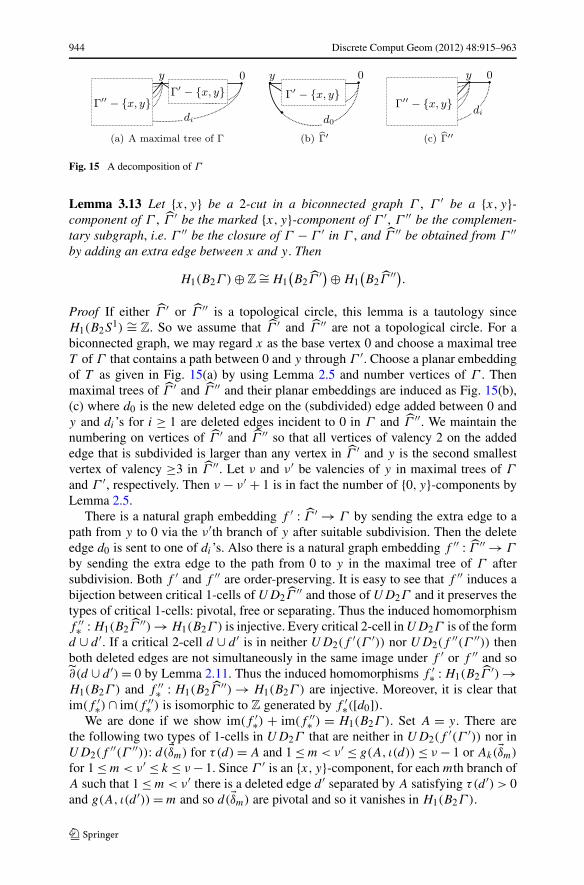
Fig. 15 A decomposition of Γ
Lemma 3.13 Let {x, y} be a 2-cut in a biconnected graph Γ , Γ ′ be a {x, y}-component of Γ , Γ ′ be the marked {x, y}-component of Γ ′, Γ ′′ be the complemen-tary subgraph, i.e. Γ ′′ be the closure of Γ − Γ ′ in Γ , and Γ ′′ be obtained from Γ ′′by adding an extra edge between x and y. Then
H1(B2Γ ) ⊕ Z ∼= H1(B2Γ
′)⊕ H1(B2Γ
′′).
Proof If either Γ ′ or Γ ′′ is a topological circle, this lemma is a tautology sinceH1(B2S
1) ∼= Z. So we assume that Γ ′ and Γ ′′ are not a topological circle. For abiconnected graph, we may regard x as the base vertex 0 and choose a maximal treeT of Γ that contains a path between 0 and y through Γ ′. Choose a planar embeddingof T as given in Fig. 15(a) by using Lemma 2.5 and number vertices of Γ . Thenmaximal trees of Γ ′ and Γ ′′ and their planar embeddings are induced as Fig. 15(b),(c) where d0 is the new deleted edge on the (subdivided) edge added between 0 andy and di ’s for i ≥ 1 are deleted edges incident to 0 in Γ and Γ ′′. We maintain thenumbering on vertices of Γ ′ and Γ ′′ so that all vertices of valency 2 on the addededge that is subdivided is larger than any vertex in Γ ′ and y is the second smallestvertex of valency ≥3 in Γ ′′. Let ν and ν′ be valencies of y in maximal trees of Γ
and Γ ′, respectively. Then ν − ν′ + 1 is in fact the number of {0, y}-components byLemma 2.5.
There is a natural graph embedding f ′ : Γ ′ → Γ by sending the extra edge to apath from y to 0 via the ν′th branch of y after suitable subdivision. Then the deleteedge d0 is sent to one of di ’s. Also there is a natural graph embedding f ′′ : Γ ′′ → Γ
by sending the extra edge to the path from 0 to y in the maximal tree of Γ aftersubdivision. Both f ′ and f ′′ are order-preserving. It is easy to see that f ′′ induces abijection between critical 1-cells of UD2Γ
′′ and those of UD2Γ and it preserves thetypes of critical 1-cells: pivotal, free or separating. Thus the induced homomorphismf ′′∗ : H1(B2Γ
′′) → H1(B2Γ ) is injective. Every critical 2-cell in UD2Γ is of the formd ∪ d ′. If a critical 2-cell d ∪ d ′ is in neither UD2(f
′(Γ ′)) nor UD2(f′′(Γ ′′)) then
both deleted edges are not simultaneously in the same image under f ′ or f ′′ and so∂(d ∪ d ′) = 0 by Lemma 2.11. Thus the induced homomorphisms f ′∗ : H1(B2Γ
′) →H1(B2Γ ) and f ′′∗ : H1(B2Γ
′′) → H1(B2Γ ) are injective. Moreover, it is clear thatim(f ′∗) ∩ im(f ′′∗ ) is isomorphic to Z generated by f ′∗([d0]).
We are done if we show im(f ′∗) + im(f ′′∗ ) = H1(B2Γ ). Set A = y. There arethe following two types of 1-cells in UD2Γ that are neither in UD2(f
′(Γ ′)) nor inUD2(f
′′(Γ ′′)): d(�δm) for τ(d) = A and 1 ≤ m < ν′ ≤ g(A, ι(d)) ≤ ν − 1 or Ak(�δm)
for 1 ≤ m < ν′ ≤ k ≤ ν − 1. Since Γ ′ is an {x, y}-component, for each mth branch ofA such that 1 ≤ m < ν′ there is a deleted edge d ′ separated by A satisfying τ(d ′) > 0and g(A, ι(d ′)) = m and so d(�δm) are pivotal and so it vanishes in H1(B2Γ ).
Discrete Comput Geom (2012) 48:915–963 945
Since {x, y} is a 2-cut, for each kth branch of A such that ν′ ≤ k ≤ ν − 1 thereis a deleted edge di such that g(A, ι(di)) = k and τ(di) = 0. Since g(τ(d ′), ι(di)) =g(τ(d ′),A) = g(τ(d ′), ι(f ′(d0))) for the deleted edge d ′ found above,
∂(d ′ ∪di −d ′ ∪f ′(d0)
)= ±(∧(
d ′, di
)±∧(
d ′, f ′(d0)))= ±(Ak(�δm)±Aν′(�δm)
)
by Lemma 3.2(3). Thus Ak(�δm) and Aν′(�δm) are homologous up to signs and Aν′(�δm)
is a critical 1-cell in UD2(f′(Γ ′)). �
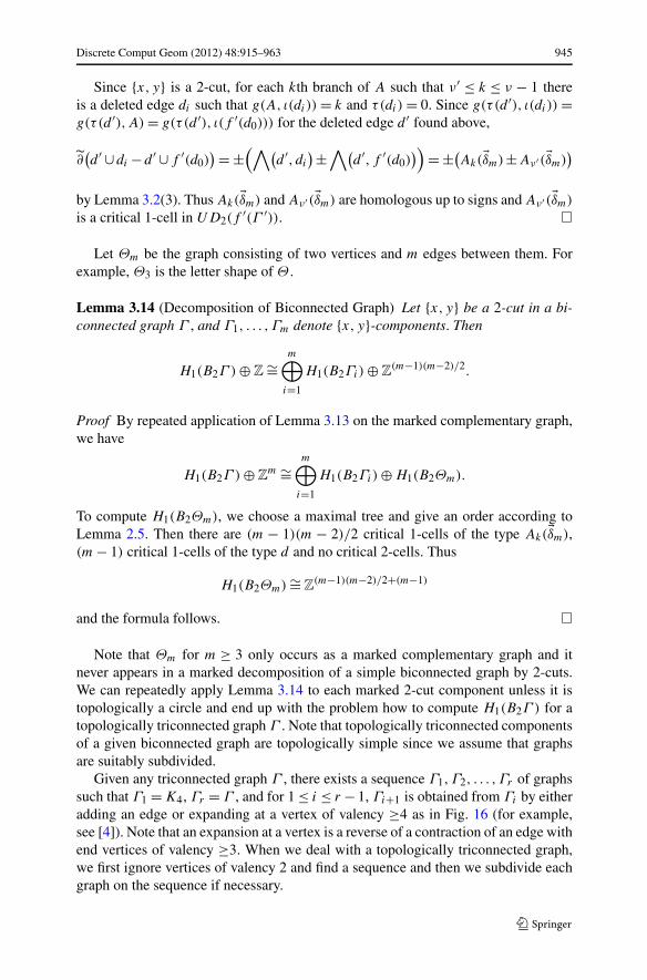
Let Θm be the graph consisting of two vertices and m edges between them. Forexample, Θ3 is the letter shape of Θ .
Lemma 3.14 (Decomposition of Biconnected Graph) Let {x, y} be a 2-cut in a bi-connected graph Γ , and Γ1, . . . ,Γm denote {x, y}-components. Then
H1(B2Γ ) ⊕ Z ∼=m⊕
i=1
H1(B2Γi) ⊕ Z(m−1)(m−2)/2.
Proof By repeated application of Lemma 3.13 on the marked complementary graph,we have
H1(B2Γ ) ⊕ Zm ∼=
m⊕
i=1
H1(B2Γi) ⊕ H1(B2Θm).
To compute H1(B2Θm), we choose a maximal tree and give an order according toLemma 2.5. Then there are (m − 1)(m − 2)/2 critical 1-cells of the type Ak(�δm),(m − 1) critical 1-cells of the type d and no critical 2-cells. Thus
H1(B2Θm) ∼= Z(m−1)(m−2)/2+(m−1)
and the formula follows. �
Note that Θm for m ≥ 3 only occurs as a marked complementary graph and itnever appears in a marked decomposition of a simple biconnected graph by 2-cuts.We can repeatedly apply Lemma 3.14 to each marked 2-cut component unless it istopologically a circle and end up with the problem how to compute H1(B2Γ ) for atopologically triconnected graph Γ . Note that topologically triconnected componentsof a given biconnected graph are topologically simple since we assume that graphsare suitably subdivided.
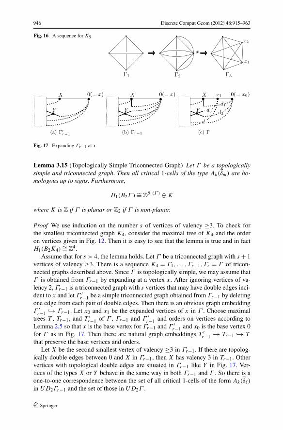
Given any triconnected graph Γ , there exists a sequence Γ1,Γ2, . . . ,Γr of graphssuch that Γ1 = K4, Γr = Γ , and for 1 ≤ i ≤ r − 1, Γi+1 is obtained from Γi by eitheradding an edge or expanding at a vertex of valency ≥4 as in Fig. 16 (for example,see [4]). Note that an expansion at a vertex is a reverse of a contraction of an edge withend vertices of valency ≥3. When we deal with a topologically triconnected graph,we first ignore vertices of valency 2 and find a sequence and then we subdivide eachgraph on the sequence if necessary.
946 Discrete Comput Geom (2012) 48:915–963
Fig. 16 A sequence for K5
Fig. 17 Expanding Γr−1 at x
Lemma 3.15 (Topologically Simple Triconnected Graph) Let Γ be a topologicallysimple and triconnected graph. Then all critical 1-cells of the type Ak(�δm) are ho-mologous up to signs. Furthermore,
H1(B2Γ ) ∼= Zβ1(Γ ) ⊕ K
where K is Z if Γ is planar or Z2 if Γ is non-planar.
Proof We use induction on the number s of vertices of valency ≥3. To check forthe smallest triconnected graph K4, consider the maximal tree of K4 and the orderon vertices given in Fig. 12. Then it is easy to see that the lemma is true and in factH1(B2K4) ∼= Z
4.Assume that for s > 4, the lemma holds. Let Γ be a triconnected graph with s + 1
vertices of valency ≥3. There is a sequence K4 = Γ1, . . . ,Γr−1,Γr = Γ of tricon-nected graphs described above. Since Γ is topologically simple, we may assume thatΓ is obtained from Γr−1 by expanding at a vertex x. After ignoring vertices of va-lency 2, Γr−1 is a triconnected graph with s vertices that may have double edges inci-dent to x and let Γ ′
r−1 be a simple triconnected graph obtained from Γr−1 by deletingone edge from each pair of double edges. Then there is an obvious graph embeddingΓ ′
r−1 ↪→ Γr−1. Let x0 and x1 be the expanded vertices of x in Γ . Choose maximaltrees T , Tr−1, and T ′
r−1 of Γ , Γr−1 and Γ ′r−1 and orders on vertices according to
Lemma 2.5 so that x is the base vertex for Γr−1 and Γ ′r−1 and x0 is the base vertex 0
for Γ as in Fig. 17. Then there are natural graph embeddings T ′r−1 ↪→ Tr−1 ↪→ T
that preserve the base vertices and orders.Let X be the second smallest vertex of valency ≥3 in Γr−1. If there are topolog-
ically double edges between 0 and X in Γr−1, then X has valency 3 in Tr−1. Othervertices with topological double edges are situated in Γr−1 like Y in Fig. 17. Ver-tices of the types X or Y behave in the same way in both Γr−1 and Γ . So there is aone-to-one correspondence between the set of all critical 1-cells of the form Ak(�δ�)
in UD2Γr−1 and the set of those in UD2Γ .
Discrete Comput Geom (2012) 48:915–963 947
By the induction hypothesis, all critical 1-cells of the form Ak(�δ�) in UD2Γ′r−1
are separating and homologous up to signs. We first find out which critical 1-cell ofthe form Ak(�δ�) in UD2Γr−1 is not separating. It is enough to check for the verticesof the type either X or Y since Ak(�δ�) can be regarded as a critical 1-cell in UD2Γ
′r−1
for all other vertices A and UD2Γr−1 has more critical 2-cells than UD2Γ′r−1. For X,
there is only one critical 1-cell X2(�δ1) and it is not separating by Lemma 3.8. Supposethe pth and the (p + 1)st branches of Y are topological double edges from Y to 0.Then Yp+1(�δp) is not separating either by Lemma 3.8. Unless k = p + 1 and � = q ,Yk(�δ�) is separating because one of the pth and the (p + 1)st branches lies on Γ ′
r−1
and so Yk(�δ�) is homologous up to signs to other separating 1-cells by the inductionhypothesis.
Finally we show that critical 1-cells of UD2Γ , X2(�δ1) and Yp(�δq) are separatingand homologous up to signs to other separating 1-cells. Let d1 (d2, respectively)be a deleted edge lying on the topological edge between 0 and X (Y , respectively)in Γ , d3 be a deleted edge lying on the topological edge between x1 and Y in Γ .Then g(Y, ι(d3)) and g(Y, ι(d2)) correspond to p and p + 1. Since Γ is topologicallytriconnected, there is a deleted edge d other than d1, d2 and d3 such that τ(d) is either0 or x1. Otherwise, {X,Y } would be a 2-cut in Γ . In fact, Fig. 17 shows examplesof d1, d2, d3, and d . Consider the following boundary images on the Morse chaincomplex of UD2Γ :For τ(d) = 0,
∂(d3 ∪ d1 − d3 ∪ d) = X2(�δ1) ±∧
(d3, d),
∂(d3 ∪ d2 − d3 ∪ d) = −Yp(�δq) ±∧
(d3, d).
For τ(d) = x2,
∂(d3 ∪ d1 − d3 ∪ d2) = X2(�δ1) + Yp(�δq),
∂(d ∪ d1 − d ∪ d2) = X2(�δ1) ±∧
(d, d2).
So[X2(�δ1)
]= −[Yp(�δq)]= ±
[∧(d3, d)
] (or ±[∧
(d, d2)])
.
Thus all critical 1-cells of the form Ak(�a) in UD2Γ are separating and homologousup to signs.
Now we consider H1(B2Γ ). Since we know that Ak(�a) are separating, free 1-cellsare of the form d for some deleted edge d by Lemma 3.7. The number of deletededges is equal to β1(Γ ). So
H1(B2Γ ) ∼= Zβ1(Γ ) ⊕ ⟨[Ak(�a)
]⟩.
It is easy to see that [Ak(�a)] is not trivial in H1(B2Γ ). If Γ is planar then [Ak(�a)]is torsion-free by Corollary 3.6. It is easy to see that if a topologically simple tri-connected graph Γ is embedded in a topologically simple triconnected graph Γ asgraphs, then the embedding induces a homomorphism: H1(B2Γ ) → H1(B2Γ ) which
948 Discrete Comput Geom (2012) 48:915–963
corresponds the homology class [Ak(�a)] to the same kind of homology classes. FromExample 3.9, [Ak(�a)] in H1(B2K5) is a 2-torsion. It is easy to check that [Ak(�a)]in H1(B2K3,3) is a 2-torsion from Example 2.1. So if Γ is a non-planar graph then[Ak(�a)] in H1(B2Γ ) generates the summand Z2. �
By combining lemmas in this section, we can give a formula for H1(BnΓ ) fora finite connected graph Γ and any braid indices using the connectivity of graphs.Recall that
N(n,Γ,x) =(
n + μ(x) − 2n − 1
)×(ν(x)−2
)−(
n + μ(x) − 2n
)−(ν(x)−μ(x)−1
)
where μ(x) is the number of x-components of Γ and ν(x) is the valency of x in Γ .Note that if ν(x) = 2 (and so μ(x) = 2), then N(n,Γ,x) = 0. Let V1(Γ ) denote a setof 1-cuts that decomposes Γ into biconnected components and copies of topologicalline segments. Define
N1(n,Γ ) =∑
x∈V1(Γ )
N(n,Γ, x).
For a biconnected graph Γ , let V2 denote a set of 2-cuts whose marked decompo-sition decomposes Γ into triconnected components and copies of topological circles.Define
N2(Γ ) =∑
{x,y}∈V2
(μ({x, y}) − 1)(μ({x, y}) − 2)
2
where μ({x, y}) denotes the number of {x, y}-components in Γ . Note that for C ∈ V2,μ(C) in Γ is equal to that in any marked D-component for D ∈ V2. And note that ifone of x and y has valency 2 for a 2-cut {x, y} ∈ V2, then μ({x, y}) = 2.
For a connected graph Γ , define N2(Γ ) =∑ki=1 N2(Γi) where Γ1, . . . ,Γk are
biconnected components of Γ .For a connected graph Γ , let N3(Γ ) (N ′
3(Γ ), respectively) be the number of tri-connected components of Γ that are planar (non-planar, respectively).
Theorem 3.16 For a finite connected graph Γ ,
H1(BnΓ ) = ZN1(n,Γ )+N2(Γ )+N3(Γ )+β1(Γ ) ⊕ Z
N ′3(Γ )
2 .
Proof By Lemmas 3.11 and 3.12 we have
H1(BnΓ ) =(⊕
i
H1(B2Γi)
)⊕ Z
N1(n,Γ )
where Γi ’s are biconnected components of Γ . Since N2(Γ ), N3(Γ ), N ′3(Γ ) and
β1(Γ ) are equal to the sum of those for Γi , it is sufficient to show that for a bi-connected graph Γ ,
H1(B2Γ ) = ZN2(Γ )+N3(Γ )+β1(Γ ) ⊕ Z
N ′3(Γ )
2 .
Discrete Comput Geom (2012) 48:915–963 949
Let V2 be a set of 2-cuts in Γ such that the marked decomposition along V2 de-composes a biconnected graph Γ into triconnected components and copies of topo-logical circles. Let {Γi} be the set of marked components obtained from Γ by cuttingalong V2. By Lemma 3.14,
H1(B2Γ ) ⊕ Z|V2| =
(⊕H1(B2Γi)
)⊕ Z
N2(Γ ).
By Lemma 3.15, H1(B2Γi) ∼= Zβ1(Γi ) ⊕ Z, Z
β1(Γi ) ⊕ Z2, or Z if Γi is a planar tricon-nected graph, a non-planar triconnected graph, or a topological circle, respectively.
Thus⊕
H1(B2Γi) ∼= ZN3(Γ )+∑β1(Γi ) ⊕ Z
N ′3(Γ )
2 . Since we are dealing with markedcomponents,
∑β1(Γi) = β1(Γ ) + |V2|. Thus H1(B2Γ ) ∼= Z
N2(Γ )+N3(Γ )+β1(Γ ) ⊕Z
N ′3(Γ )
2 . �
It seems difficult to compute higher homology groups of BnΓ in general. How-ever, UD2Γ is a 2-dimensional complex and so H2(B2Γ ) is torsion-free. And thesecond Betti number of B2Γ is given as follows:
Corollary 3.17 For a finite connected graph Γ ,
β2(B2Γ ) = N1(n,Γ ) + N2(Γ ) + N3(Γ ) − 1
2
∑
x∈V (Γ )
(ν(x) − 1
)(ν(x) − 2
)
+ 1
2β1(Γ )
(β1(Γ ) − 1
)+ 2.
Proof We choose a maximal tree such that two end vertices of every deleted edgehave valency 2. Then the number of critical 2-cells is equal to 1
2β1(Γ )(β1(Γ ) − 1)
and the number of critical 1-cells is 12
∑x∈V (Γ )(ν(x)− 1)(ν(x)− 2)+β1(Γ ). Using
Euler characteristic of the Morse chain complex, we have
1 − β1(B2Γ ) + β2(B2Γ )
= 1 − 1
2
∑
x∈V (Γ )
(ν(x) − 1
)(ν(x) − 2
)− β1(Γ ) + 1
2β1(Γ )
(β1(Γ ) − 1
).
We use β1(B2Γ ) = N1(n,Γ ) + N2(Γ ) + N3(Γ ) + β1(Γ ) to complete the proof. �
3.3 The Homologies of Pure Graph 2-Braid Groups
In Sect. 2.2, we describe a Morse chain complex MnΓ of DnΓ . The technologydeveloped for UDnΓ in this article is not enough to compute H1(PnΓ ). For example,the boundary image of (Ak(�a)∪B�(�b))σ never vanishes in MnΓ for n ≥ 4. However,for braid index 2 the second boundary map behaves in the way similar to unorderedcases. This is because there are only one type critical 2-cells (d ∪ d ′)σ .
In general, the image of cσ under R or ∂ is obtained by right multiplication by σ onthe permutation subscript of each term in the image of cid. For example, if R(cid) =
950 Discrete Comput Geom (2012) 48:915–963
∑i (ci)τi
then R(cσ ) =∑i (ci)τiσ . Thus we only consider cid. We will discuss 2-braidgroups in this section and ρ denotes the nontrivial permutation in S2.
We have the following lemma for D2Γ that is similar to Lemma 2.3 for UDnΓ
but it is hard to have a lemma corresponding to Lemma 2.4.
Lemma 3.18 (Special Reduction) Suppose a redundant 1-cell cid in D2Γ has a sim-ple unblocked vertex. Then R(cid) = R(V (c)id).
Proof Let e and v be the edge and the vertex in c. Since c contains only one vertex,v is the smallest unblocked vertex. Let ev be the edge starting from v. Then
R(cid) = V (c)id + {ev, ι(e)}ρm − {ev, τ (e)
}id
where m is 1 if τ(e) < v < ι(e) or 0 otherwise.We use induction on i such that Ri(cid) = Ri+1(cid). Since cid is redundant,
i ≥ 2. Since V ({ev, ι(e)}ρm) = {ev, τ (e)}ρ2m , RV ({ev, ι(e)}ρm) = R({ev, τ (e)}ρ2m)
by induction hypothesis. Thus R({ev, ι(e)}ρm − {ev, τ (e)}id) = RV ({ev, ι(e)}ρm) −R({ev, τ (e)}id) = 0. Thus R(cid) = R(V (c)id). �
Since all critical 2-cells in DΓ is of the form (d ∪d ′)σ , we only need the following:
Lemma 3.19 (Boundary Formulae) Let c = d ∪ d ′, τ(d) > τ(d ′), k = g(τ(d), ι(d))
and � = g(τ(d), ι(d ′)).
(a) If d ′ is separated by τ(d), k �= � and ι(d) < ι(d ′) then
∂(cid) = did − d(�δ�)ρ.
(b) If d ′ is separated by τ(d), k = � and ι(d) < ι(d ′) then
∂(cid) = did − d(�δ�)ρ −∧(
d, d ′)id.
(c) If d ′ is separated by τ(d) and ι(d ′) < ι(d) then
∂(cid) = did − d(�δ�)ρ +∧(
d, d ′)ρ.
(d) Otherwise ∂(cid) = 0.
Proof It is sufficient to compute images under R for each boundary 1-cell after ob-taining the boundary of cid in D2Γ .
If ι(d ′) < τ(d), then
∂((
d ∪ d ′)id
)= (d ∪ {τ(d ′)})id − (d ∪ {ι(d ′)})
id + (d ′ ∪ {ι(d)})
id − (d ′ ∪ {τ(d)})
id.
By Lemma 3.18 we have R((d ∪{τ(d ′)})id) = R((d ∪{ι(d ′)})id) = did. Since ι(d ′) <
τ(d) < ι(d), we have R((d ′ ∪ {ι(d)})id) = d ′ ∪ {τ(d)}id. So if ι(d ′) < τ(d), then∂((d ∪ d ′)id) = 0.
Discrete Comput Geom (2012) 48:915–963 951
If ι(d ′) > τ(d), then
∂((
d ∪ d ′)id
)= (d ∪ {τ(d ′)})id − (d ∪ {ι(d ′)})
ρ+ (d ′ ∪ {ι(d)
})id − (d ′ ∪ {τ(d)
})id.
Let B = ι(d ′) ∧ τ(d) and m = g(B, ι(d ′)). If d ′ is not separated by τ(d) then ι(d ′) >
ι(d) from g(B, ι(d ′)) > g(B, τ(d)) = g(B, ι(d)). So we have R((d ′ ∪ {ι(d)})id) =(d ′ ∪ {τ(d)})id and
R((
d ∪ {ι(d ′)})ρ
)= R((
d ∪ B(�δm))ρ
)
= R((
d ∪ {B})id + (Bm ∪ {ι(d)})
id − (Bm ∪ {τ(d)})
id
)
= R((
d ∪ {B})id)= R
((d ∪ {τ(d ′)})
id
),
since R((Bm ∪ {ι(d)})id) = R((Bm ∪ {τ(d)})id) by Lemma 3.18. So if ι(d ′) > τ(d)
and d ′ is not separated by τ(d), then ∂((d ∪ d ′)id) = 0.Let q = g(τ(d ′), τ (d)). If d ′ is separated by τ(d), then it is easy to see that
R((
d ∪ {τ(d ′)})id
)= did and R((
d ′ ∪ {τ(d)})
id
)= d ′(�δq)id.
Let C = ι(d ′)∧ ι(d) and m1 = g(C, ι(d ′)). Consider R((d ∪{ι(d ′)})ρ). If either k �= �
or k = � and ι(d ′) < ι(d), then R((d ∪ {ι(d ′)})ρ) = d(�δ�)ρ by Lemma 3.18. If k = �
and ι(d) < ι(d ′), then by Lemma 3.18,
R((
d ∪ {ι(d ′)})ρ
)= R((
d ∪ C(�δm1))ρ
)
= R((
d ∪ {C})ρ
+ (Cm1 ∪ {ι(d)})
id − (Cm1 ∪ {τ(d)})
ρ
)
= R((
d ∪ {C})ρ
+ (Cm1 ∪ {ι(d)})
id
)= d(�δ�)ρ +∧(
d, d ′)id.
Let m2 = g(C, ι(d)). Finally consider R((d ′ ∪ {ι(d)})id). If ι(d) < ι(d ′) thenR((d ′ ∪ {ι(d)})id) = d ′(�δq)id. If ι(d ′) < ι(d), then
R((
d ′ ∪ {ι(d)})
id
)= R((
d ′ ∪ C(�δm2))
id
)
= R((
d ′ ∪ {C})id + (Cm2 ∪ {ι(d)})
ρ− (Cm2 ∪ {τ(d)
})id
)
= R((
d ′ ∪ {C})id + (Cm2 ∪ {ι(d)})
ρ
)= d(�δ�)id +∧(
d, d ′)ρ.
Combining the results, we obtain the desired formulae. �
Using the above lemma, we have the following lemma similar to Lemma 3.2.
Lemma 3.20 (Dependence Among Boundary Images) If d1 and d2 are separated byτ(d) and g(τ(d), ι(d1)) = g(τ(d), ι(d2)), then
(1) If g(τ(d), ι(d)) �= g(τ(d), ι(d1)), then ∂((d ∪ d1)id) = ∂((d ∪ d2)id).(2) If g(τ(d), ι(d)) = g(τ(d), ι(d1)), then
∂((d ∪ d1)id − (d ∪ d2)id
)= −(−1)i ∧ (d, d1)ρi + (−1)j ∧ (d, d2)ρj .
952 Discrete Comput Geom (2012) 48:915–963
Note that the second formula of the above lemma contains i, j only for the paritypurpose and plays an important role of showing that H1(P2Γ ) is torsion-free.
Declare an order on S2 by id > ρ. Recall the orders on critical 1-cells and critical2-cells of UDnΓ from Sect. 3.1. By adding a permutation as the last componentof the orders, we obtain orders given by 4-tuples (s(c), e, �a,σ ) for critical 1-cellsin D2Γ and by 7-tuples (s(c), e, �a + �δg(τ(e),ι(e′)), g(τ (e), ι(e′)), e′, �b,σ ) for critical2-cells.
The second boundary homomorphism ∂ is represented by a matrix over bases ofcritical 2-cells and critical 1-cells ordered reversely. We go through the exactly samearguments as in Sect. 3.1 by using Lemmas 3.20 and 3.19 and obtain the followingtheorem:
Theorem 3.21 Let M be the matrix representing the second boundary homomor-phism of D2Γ over bases of critical 2-cells and critical 1-cells ordered reversely. Upto row operations, each row of M satisfies one of the following:
(1) it consists of all zeros;(2) there is a ±1 entry that is the only nonzero entry in the column it belongs to;(3) there are only two nonzero entries which are ±1.
Furthermore, up to multiplications of column by −1, the property (3) above can bemodified to
(3′) there are two nonzero entries which are ±1 and have opposite signs.
Proof Lemma 3.20 (2) implies that (3′) can be achieved by choosing a basis of critical1-cells in which (−1)mcρm is used instead of just cid or cρ . �
Since there are exactly two critical 0-cells, the 0th skeleton (M2Γ )0 of a Morsecomplex of M2Γ of D2Γ consists of two points. Then the second boundary ho-momorphism gives a presentation matrix for H1(M2Γ, (M2Γ )0). And H1(M2Γ,
(M2Γ )0) ∼= H1(M2Γ ) ⊕ Z ∼= H1(P2Γ ) ⊕ Z.Critical 1-cells of D2Γ can be classified to be pivotal, free, or separating as before.
The undetermined block of separating 1-cells produces no torsion due to the property(3′) and so we have the following:
Corollary 3.22 For a finite connected graph Γ , H1(P2Γ ) is torsion-free.
Using free 1-cells and the undetermined block for H1(M2Γ, (M2Γ )0), we cancompute H1(P2Γ ).
Example 3.23 Let Γ be K5 and a maximal tree and an order be given as in Exam-ple 2.6. We want to compute H1(P2Γ ).
From ∂(d6 ∪ d5 − d6 ∪ d2) = −C2(1,0,0) − B3(0,1,0) in Example 3.9, we obtain
∂((d6 ∪ d5)id − (d6 ∪ d4)id
)= −C2(1,0,0)id + {−B3(0,1,0)ρ}.
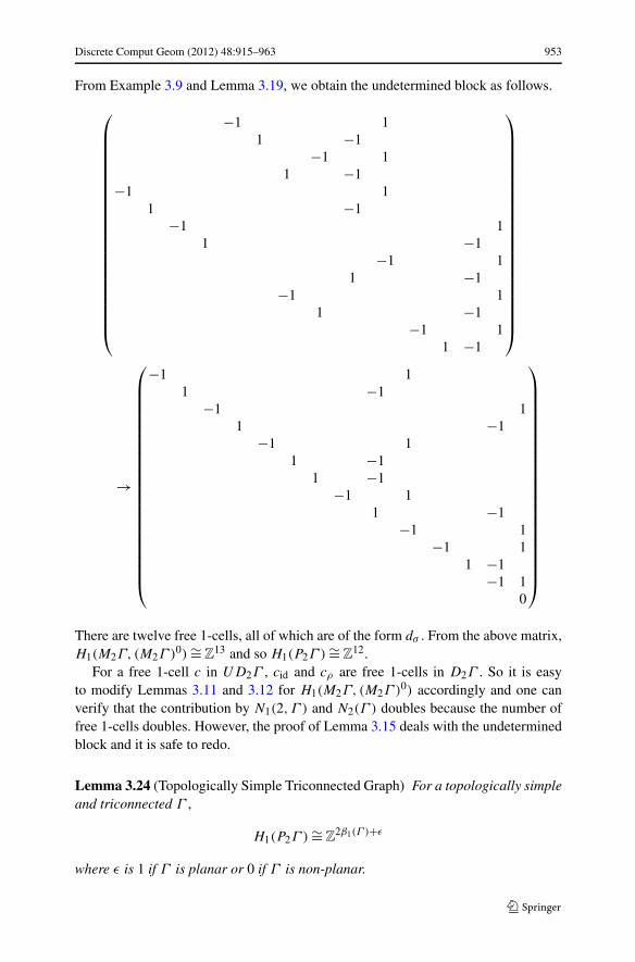
Discrete Comput Geom (2012) 48:915–963 953
From Example 3.9 and Lemma 3.19, we obtain the undetermined block as follows.
⎛
⎜⎜⎜⎜⎜⎜⎜⎜⎜⎜⎜⎜⎜⎜⎜⎜⎜⎜⎜⎜⎜⎜⎝
−1 11 −1
−1 11 −1
−1 11 −1
−1 11 −1
−1 11 −1
−1 11 −1
−1 11 −1
⎞
⎟⎟⎟⎟⎟⎟⎟⎟⎟⎟⎟⎟⎟⎟⎟⎟⎟⎟⎟⎟⎟⎟⎠
→
⎛
⎜⎜⎜⎜⎜⎜⎜⎜⎜⎜⎜⎜⎜⎜⎜⎜⎜⎜⎜⎜⎜⎜⎝
−1 11 −1
−1 11 −1
−1 11 −1
1 −1−1 1
1 −1−1 1
−1 11 −1
−1 10
⎞
⎟⎟⎟⎟⎟⎟⎟⎟⎟⎟⎟⎟⎟⎟⎟⎟⎟⎟⎟⎟⎟⎟⎠
There are twelve free 1-cells, all of which are of the form dσ . From the above matrix,H1(M2Γ, (M2Γ )0) ∼= Z
13 and so H1(P2Γ ) ∼= Z12.
For a free 1-cell c in UD2Γ , cid and cρ are free 1-cells in D2Γ . So it is easyto modify Lemmas 3.11 and 3.12 for H1(M2Γ, (M2Γ )0) accordingly and one canverify that the contribution by N1(2,Γ ) and N2(Γ ) doubles because the number offree 1-cells doubles. However, the proof of Lemma 3.15 deals with the undeterminedblock and it is safe to redo.
Lemma 3.24 (Topologically Simple Triconnected Graph) For a topologically simpleand triconnected Γ ,
H1(P2Γ ) ∼= Z2β1(Γ )+ε
where ε is 1 if Γ is planar or 0 if Γ is non-planar.
954 Discrete Comput Geom (2012) 48:915–963
Proof We need to show that H1(M2Γ, (M2Γ )0) ∼= Z2β1(Γ )+ε+1. Critical 1-cells are
of the forms dσ , d(δ�)σ and Ak(�δ�)σ with k > �. It is easy to see that every crit-ical 1-cell of the form d(δ�)σ is pivotal and the number of critical 1-cells of theform dσ is equal to 2β1(Γ ). We consider the undetermined block. From the proofof Lemma 3.15, there are at most two homology classes of the form [Ak(�δ�)id]and [Ak(�δ�)ρ]. So it is sufficient to show that [Ak(�δ�)id] �= [Ak(�δ�)ρ] if Γ is pla-nar and [Ak(�δ�)id] = [Ak(�δ�)ρ] if Γ is non-planar. If Γ is planar, then by condi-tion (T4) in Lemma 2.12, there is no row representing ±{Ak(�δ�)id + Bk′(�δ�′)ρ}. So[Ak(�δ�)id] �= [Ak(�δ�)ρ]. For non-planar graphs, we only need to verify for K5 andK3,3 as was explained in the proof of Lemma 3.15. Examples 2.2 and 3.23 show thatH1(P2K5) and H1(P2K3,3) satisfy the lemma. �
Using the same arguments in the proof of Theorem 3.16, we obtain the formula
H1(M2Γ, (M2Γ )0)∼= Z
2N1(2,Γ )+2N2(Γ )+2N3(Γ )+2β1(Γ )+N ′3(Γ ).
This implies the following theorem.
Theorem 3.25 For a finite connected graph Γ ,
H1(P2Γ ) ∼= Z2N1(2,Γ )+2N2(Γ )+2N3(Γ )+2β1(Γ )+N ′
3(Γ )−1.
Since there are no critical i-cells for i ≥ 3 in D2Γ , H∗(P2Γ ) is torsion-free. Sowe can compute H2(P2Γ ) as follows. Choose a maximal tree such that two endvertices of every deleted edge have valency 2. Then there are two critical 0-cellsand β1(Γ )(β1(Γ ) − 1) critical 2-cells and the number of critical 1-cells is equal to∑
x∈V (Γ )(ν(x) − 1)(ν(x) − 2) + 2β1(Γ ). So we have the second Betti number ofP2Γ as follows:
β2(P2Γ ) = 2N1(2,Γ ) + 2N2(Γ ) + 2N3(Γ ) + N ′3(Γ ) + β1(Γ )
(β1(Γ ) − 1
)
−∑
x∈V (Γ )
(ν(x) − 1
)(ν(x) − 2
).
A formula for β1(P2Γ ) − β2(P2Γ ) was given by Barnett and Farber in [3].As a closing thought of this section, it is tempting to use Lyndon–Hochschild–
Serre spectral sequence for Sn = BnΓ/PnΓ to extract some information aboutH1(PnΓ ) via homologies of the other two groups. In fact, we have the exact sequence
H2(BnΓ ) → H2(Sn) → H1(PnΓ )Sn → H1(BnΓ ) → H1(Sn) → 0
where H1(PnΓ )Sn is isomorphic to H1(PnΓ )/IH1(PnΓ ) as Z[Sn]-modules and I isthe kernel of the augmentation Z[Sn] → Z. Even though the action on critical 1-cellsby Sn is clearly understood, the action on homology classes is not so clear withoutany information about the second boundary map.
Discrete Comput Geom (2012) 48:915–963 955
4 Applications and More Characteristics of Graph Braid Groups
In this section we first discuss consequences of the formulae obtained in the previoussection. Then we develop a technology for graph braid groups themselves that isparallel to the technology successfully applied for the first homologies of graph braidgroups. And we discover more characteristics of graph braid groups and pure braidgroups beyond their homologies. These characteristics are defined by weakening therequirement for right-angled Artin groups.
4.1 Planar and Non-planar Triconnected Graphs
Since we are not interested in trivial graphs such as a topological line segment of atopological circle, we assume Γ has at least a vertex of valency ≥3 in this discus-sion. For any 1-cut x of valency ≥3, N(n,Γ,x) > 0. Thus N1(n,Γ ) = 0 if and only ifthere is no 1-cut of valency ≥3 if and only if Γ is biconnected. If N2(Γ ) = 0 for a bi-connected graph Γ , then μ({x, y}) = 2 for every 2-cut {x, y}. If Γ has multiple edgesbetween vertices x and y after ignoring vertices with valency 2, then μ({x, y}) > 2for some 2-cut {x, y} and so N2(Γ ) > 0. Thus if N2(Γ ) = 0 for a biconnected graph,then Γ is topologically simple. If N3(Γ ) = N ′
3(Γ ) = 0, then Γ does not topologi-cally contain the complete graph K4 by the construction of triconnected graphs. IfN1(n,Γ ) = N2(Γ ) = 0 and N3(Γ )+N ′
3(Γ ) = 1, then Γ is topologically simple andtriconnected.
Barnett and Farber proved in [3] that if for a finite connected planar graph Γ
with no vertices of valency ≤2 that is embedded in R2, the connected components
U0,U1, . . . ,Ur of the complement R2 − p(Γ ) with the unbounded component U0
satisfy the conditions that
(i) the closure of every domain Ui>0 is contractible and U0 is homotopy equivalentto S1, and
(ii) for every i, j ∈ {1, . . . , r}, Ui ∩ Uj is connected,
then β1(D2Γ ) = 2β1(Γ ) + 1.Condition (i) implies that Γ has no 1-cut. Condition (ii) implies that either
Γ is the Θ-shape graph if |V (Γ )| = 2 or Γ has neither multiple edges nor2-cuts if |V (Γ )| > 2. So the hypotheses imply that Γ is either the Θ-shape graphor a planar simple triconnected graph. Thus Theorem 3.25 covers this result.Furthermore, for any planar graph Γ , β1(P2Γ ) = 2β1(Γ ) + 1 if and only ifN1(2,Γ ) + N2(Γ ) + N3(Γ ) = 1 and N ′
3(Γ ) = 0. There are three nonnegative so-lutions: (N1(2,Γ ),N2(Γ ),N3(Γ )) = (1,0,0), (0,1,0) and (0,0,1).
In the case of (1,0,0), Γ has only one 1-cut vertex of valency 3. So Γ is eitherthe Y -shape tree or the P -shape graph. In the case of (0,1,0), Γ is biconnected andhas only one 2-cut {x, y} with μ({x, y}) = 3. So Γ is the Θ-shape graph. Finally, thesolution (0,0,1) implies that Γ is topologically simple and triconnected. Thus for aconnected planar graph Γ with no vertices of valency ≤2, β1(P2Γ ) = 2β1(Γ ) + 1 ifand only if Γ is either the Θ-shape graph or a simple triconnected graph. Note thatwe cannot remove the assumption of being planar because there is a counterexamplegiven in Fig. 18.
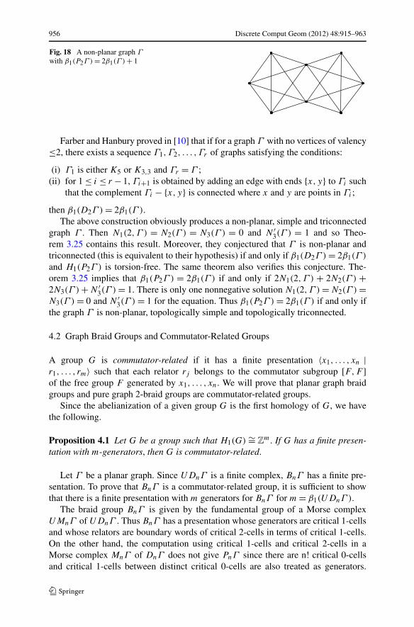
956 Discrete Comput Geom (2012) 48:915–963
Fig. 18 A non-planar graph Γ
with β1(P2Γ ) = 2β1(Γ ) + 1
Farber and Hanbury proved in [10] that if for a graph Γ with no vertices of valency≤2, there exists a sequence Γ1,Γ2, . . . ,Γr of graphs satisfying the conditions:
(i) Γ1 is either K5 or K3,3 and Γr = Γ ;(ii) for 1 ≤ i ≤ r − 1, Γi+1 is obtained by adding an edge with ends {x, y} to Γi such
that the complement Γi − {x, y} is connected where x and y are points in Γi ;
then β1(D2Γ ) = 2β1(Γ ).The above construction obviously produces a non-planar, simple and triconnected
graph Γ . Then N1(2,Γ ) = N2(Γ ) = N3(Γ ) = 0 and N ′3(Γ ) = 1 and so Theo-
rem 3.25 contains this result. Moreover, they conjectured that Γ is non-planar andtriconnected (this is equivalent to their hypothesis) if and only if β1(D2Γ ) = 2β1(Γ )
and H1(P2Γ ) is torsion-free. The same theorem also verifies this conjecture. The-orem 3.25 implies that β1(P2Γ ) = 2β1(Γ ) if and only if 2N1(2,Γ ) + 2N2(Γ ) +2N3(Γ ) + N ′
3(Γ ) = 1. There is only one nonnegative solution N1(2,Γ ) = N2(Γ ) =N3(Γ ) = 0 and N ′
3(Γ ) = 1 for the equation. Thus β1(P2Γ ) = 2β1(Γ ) if and only ifthe graph Γ is non-planar, topologically simple and topologically triconnected.
4.2 Graph Braid Groups and Commutator-Related Groups
A group G is commutator-related if it has a finite presentation 〈x1, . . . , xn |r1, . . . , rm〉 such that each relator rj belongs to the commutator subgroup [F,F ]of the free group F generated by x1, . . . , xn. We will prove that planar graph braidgroups and pure graph 2-braid groups are commutator-related groups.
Since the abelianization of a given group G is the first homology of G, we havethe following.
Proposition 4.1 Let G be a group such that H1(G) ∼= Zm. If G has a finite presen-
tation with m-generators, then G is commutator-related.
Let Γ be a planar graph. Since UDnΓ is a finite complex, BnΓ has a finite pre-sentation. To prove that BnΓ is a commutator-related group, it is sufficient to showthat there is a finite presentation with m generators for BnΓ for m = β1(UDnΓ ).
The braid group BnΓ is given by the fundamental group of a Morse complexUMnΓ of UDnΓ . Thus BnΓ has a presentation whose generators are critical 1-cellsand whose relators are boundary words of critical 2-cells in terms of critical 1-cells.On the other hand, the computation using critical 1-cells and critical 2-cells in aMorse complex MnΓ of DnΓ does not give PnΓ since there are n! critical 0-cellsand critical 1-cells between distinct critical 0-cells are also treated as generators.
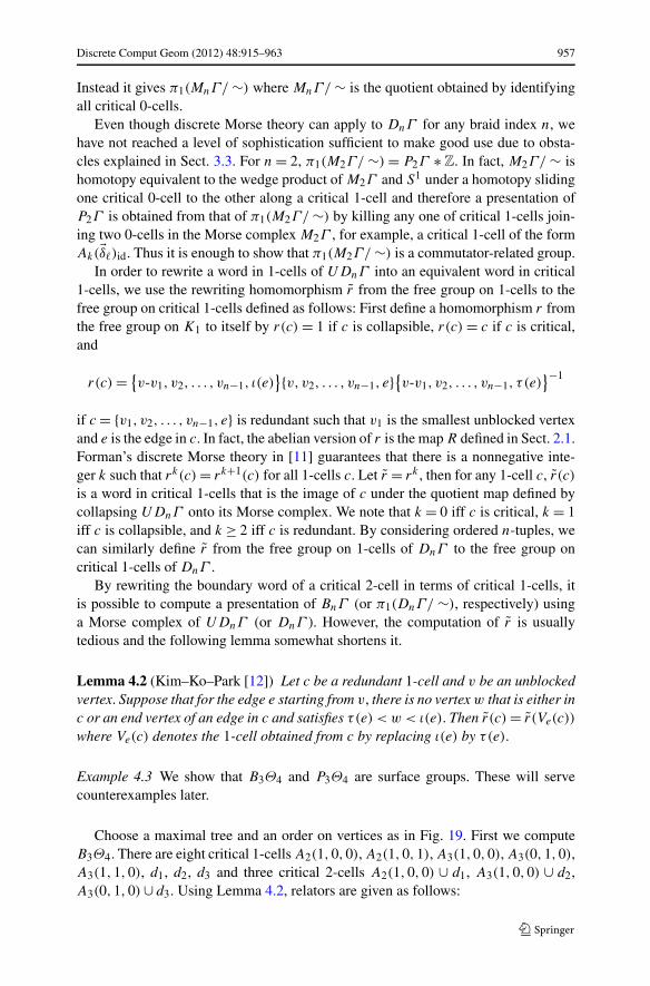
Discrete Comput Geom (2012) 48:915–963 957
Instead it gives π1(MnΓ/ ∼) where MnΓ/ ∼ is the quotient obtained by identifyingall critical 0-cells.
Even though discrete Morse theory can apply to DnΓ for any braid index n, wehave not reached a level of sophistication sufficient to make good use due to obsta-cles explained in Sect. 3.3. For n = 2, π1(M2Γ/ ∼) = P2Γ ∗ Z. In fact, M2Γ/ ∼ ishomotopy equivalent to the wedge product of M2Γ and S1 under a homotopy slidingone critical 0-cell to the other along a critical 1-cell and therefore a presentation ofP2Γ is obtained from that of π1(M2Γ/ ∼) by killing any one of critical 1-cells join-ing two 0-cells in the Morse complex M2Γ , for example, a critical 1-cell of the formAk(�δ�)id. Thus it is enough to show that π1(M2Γ/ ∼) is a commutator-related group.
In order to rewrite a word in 1-cells of UDnΓ into an equivalent word in critical1-cells, we use the rewriting homomorphism r from the free group on 1-cells to thefree group on critical 1-cells defined as follows: First define a homomorphism r fromthe free group on K1 to itself by r(c) = 1 if c is collapsible, r(c) = c if c is critical,and
r(c) = {v-v1, v2, . . . , vn−1, ι(e)}{v, v2, . . . , vn−1, e}
{v-v1, v2, . . . , vn−1, τ (e)
}−1
if c = {v1, v2, . . . , vn−1, e} is redundant such that v1 is the smallest unblocked vertexand e is the edge in c. In fact, the abelian version of r is the map R defined in Sect. 2.1.Forman’s discrete Morse theory in [11] guarantees that there is a nonnegative inte-ger k such that rk(c) = rk+1(c) for all 1-cells c. Let r = rk , then for any 1-cell c, r(c)is a word in critical 1-cells that is the image of c under the quotient map defined bycollapsing UDnΓ onto its Morse complex. We note that k = 0 iff c is critical, k = 1iff c is collapsible, and k ≥ 2 iff c is redundant. By considering ordered n-tuples, wecan similarly define r from the free group on 1-cells of DnΓ to the free group oncritical 1-cells of DnΓ .
By rewriting the boundary word of a critical 2-cell in terms of critical 1-cells, itis possible to compute a presentation of BnΓ (or π1(DnΓ/ ∼), respectively) usinga Morse complex of UDnΓ (or DnΓ ). However, the computation of r is usuallytedious and the following lemma somewhat shortens it.
Lemma 4.2 (Kim–Ko–Park [12]) Let c be a redundant 1-cell and v be an unblockedvertex. Suppose that for the edge e starting from v, there is no vertex w that is either inc or an end vertex of an edge in c and satisfies τ(e) < w < ι(e). Then r(c) = r(Ve(c))
where Ve(c) denotes the 1-cell obtained from c by replacing ι(e) by τ(e).
Example 4.3 We show that B3Θ4 and P3Θ4 are surface groups. These will servecounterexamples later.
Choose a maximal tree and an order on vertices as in Fig. 19. First we computeB3Θ4. There are eight critical 1-cells A2(1,0,0), A2(1,0,1), A3(1,0,0), A3(0,1,0),A3(1,1,0), d1, d2, d3 and three critical 2-cells A2(1,0,0) ∪ d1, A3(1,0,0) ∪ d2,A3(0,1,0) ∪ d3. Using Lemma 4.2, relators are given as follows:
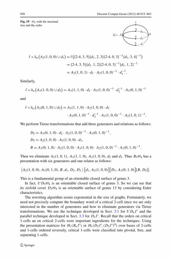
958 Discrete Comput Geom (2012) 48:915–963
Fig. 19 Θ4 with the maximaltree and the order
r ◦ ∂w
(A2(1,0,0) ∪ d1
)= r({2-4,3,5}{d1,2,3}{2-4,0,3}−1{d1,3,4}−1)
= {2-4,3,5}{d1,1,2}{2-4,0,3}−1{d1,1,2}−1
= A2(1,0,1) · d1 · A2(1,0,0)−1 · d−11 .
Similarly,
r ◦ ∂w
(A3(1,0,0) ∪ d2
)= A3(1,1,0) · d2 · A3(1,0,0)−1 · d−12 · A3(0,1,0)−1
and
r ◦ ∂w
(A3(0,1,0) ∪ d3
)= A3(1,1,0) · A2(1,0,0) · d3
· A3(0,1,0)−1 · d−13 · A3(1,0,0)−1 · A2(1,0,1)−1.
We perform Tietze transformations that add three generators and relations as follows:
D2 = A3(0,1,0) · d2 · A2(1,0,0)−1 · A3(0,1,0)−1,
D3 = A2(1,0,0) · A3(1,0,0) · d3,
B = A3(0,1,0) · A2(1,0,0) · A3(1,0,0) · A2(1,0,0)−1 · A3(0,1,0)−1.
Then we eliminate A2(1,0,1), A3(1,1,0), A3(1,0,0), d2 and d3. Thus B3Θ4 has apresentation with six generators and one relator as follows:
⟨A2(1,0,0),A3(0,1,0),B, d1,D2,D3
∣∣ [d1,A2(1,0,0)][
D3,A3(0,1,0)][B,D2]
⟩.
This is a fundamental group of an orientable closed surface of genus 3.In fact, UD3Θ4 is an orientable closed surface of genus 3. So we can see that
its sixfold cover D3Θ4 is an orientable surface of genus 13 by considering Eulercharacteristics.
The rewriting algorithm seems exponential in the size of graphs. Fortunately, weneed not precisely compute the boundary word of a critical 2-cell since we are onlyinterested in the number of generators and how to eliminate generators via Tietzetransformations. We use the technique developed in Sect. 3.1 for UDnΓ and theparallel technique developed in Sect. 3.3 for D2Γ . Recall that the orders on critical1-cells an on critical 2-cells were important ingredients for the techniques. Usingthe presentation matrices for H1(BnΓ ) or H1(D2Γ, (D2Γ )0) over bases of 2-cellsand 1-cells ordered reversely, critical 1-cells were classified into pivotal, free, andseparating 1-cells.
Discrete Comput Geom (2012) 48:915–963 959
Lemma 4.4 (Elimination of Pivotal 1-Cells) Assume that Γ has a maximal tree andan order according to Lemma 2.5. Then BnΓ and π1(D2Γ/ ∼) are generated by freeand separating 1-cells.
Proof There is no difference between BnΓ and π1(D2Γ/ ∼) in our argument. Wediscuss only BnΓ . The proof for π1(D2Γ/ ∼) is exactly the same except the fact thatpermutations are used as subscripts to express critical cells.
Consider pairs (c2, c1) of a pivotal 2-cell c2 that produces a pivotal 1-cell c1. Theneither s(c1) ≥ 2 or c1 is of the form d(�δ�). In Sect. 3.1, a pivotal 1-cell c1 is the largestsummand of ∂(c2) and so is not a summand of ∂(c′
2) for a pivotal 2-cell c′2 < c2. We
want to obtain the corresponding noncommutative version.We need to slightly modify the order on critical 1-cells when only pivotal 1-cells
are compared. For an edge e in Γ , set t (e) = 0 if e is in the maximal tree T andt (e) = 1 otherwise. Declare e > e′ if (τ (e), t (e), ι(e)) > (τ(e′), t (e′), ι(e′)). The setof pivotal 1-cells are linearly ordered by the triple (s(c), e, �a) under the modifiedorder on edges. We modified the order on the set of pivotal 2-cells accordingly, thatis, c2 > c′
2 for pivotal 2-cells c2 and c′2 if c1 > c′
1 when (c2, c1) and (c′2, c
′1) are pairs
of a pivotal 2-cell and the corresponding pivotal 1-cell.Let ∂w(c) denote the boundary word of a given pivotal 2-cell c. We claim the
following:
(a) c1 appears in the word r ◦ ∂w(c2) exactly once (as a letter or the inverse of aletter).
(b) Under the order defined above, c1 is the largest of pivotal 1-cells appeared inr ◦ ∂w(c2)
Note that (b) implies that c1 does not appear in r ◦ ∂w(c′2) for any pivotal 2-cell
c′2 < c2. Then, via Tietze transformations, we can inductively eliminate pivotal 1-cells
from the set of generators given by critical 1-cells in UDnΓ . Thus BnΓ is generatedby free and separating 1-cells. Note that it is easy to perform inductive eliminationsof pivotal 1-cells in decreasing order because no substitution is required.
To show our claim, we have to analyze each term in ∂w(c2) due to the lack ofluxury such as Lemmas 2.9 and 2.11. First consider the image of a redundant 1-cellunder r . Let c = {e, v1, . . . , vn−1} be a 1-cell. Repeated applications of Lemma 4.2imply that for any critical 1-cell c′ = {e′, v′
1, . . . , v′n−1} appearing in r(c), the vertex
τ(e′) is of valency ≥3 in Γ and of the form vi ∧ vj or vi ∧ τ(e) or vi ∧ ι(e) and,moreover, s(c′) is less than or equal to the number of vertices that do not lie on the0th branch of τ(e′) among v1, . . . , vn−1, ι(e), and τ(e). By Lemma 3.3, if c′ containsa deleted edge, then c also contains a deleted edge and c′ appears only once in r(c).And the terminal vertex of the edge in c1 is the larger one between terminal verticesof two edges in c2.
Since c2 is pivotal, the edge in c2 with the smaller terminal vertex blocks no ver-tices (see the proof of Lemma 3.4), there are two possibilities for ∂w(c2) as follows:
∂w
(Ak(�a) ∪ d ′)= Ak(�a) ∪ ι
(d ′) · d ′ ∪ A(�a) · {Ak(�a) ∪ τ
(d ′)}−1
· {d ′ ∪ A(�a + �δk)}−1
,
960 Discrete Comput Geom (2012) 48:915–963
∂w
(d(�a) ∪ d ′)= d(�a) ∪ ι
(d ′) · d ′ ∪ A(�a) · {d(�a) ∪ τ
(d ′)}−1
· {d ′ ∪ A(�a) ∪ ι(d)}−1
,
where A = τ(d) and k = g(A, ι(d)). Let c be a redundant 1-cell in the above bound-ary words, e be the edge in c, and v be a vertex of valency ≥3 in Γ other than the basevertex 0. Then the number of vertices that do not lie on the 0th branch of v amongvertices in c and end vertices of e is less than or equal to s(c2) + 1.
In the case of c2 = Ak(�a) ∪ d ′, the corresponding pivotal 1-cell c1 is Ak(�a +�δg(A,ι(d ′))) by Lemma 3.3. Repeated application of Lemma 4.2 implies r(Ak(�a) ∪ι(d ′)) = c1. Consider other three redundant 1-cells. Since s(c1) = s(c2) + 1 andτ(d ′) ∧ A = τ(d ′) < A, the words r(d ′ ∪ A(�a)) and r(Ak(�a) ∪ τ(d ′)) contain nopivotal 1-cells >c1. Since d ′ ∪ A(�a + �δk) contains a vertex <ι(Ak), ai ≥ 1 for somei < k, that is, p(�a) < k. If c = Ap(�a)(�a+�δk −�δp(�a) +�δg(A,ι(d ′))) is pivotal then c < c1.This implies that r(d ′ ∪ A(�a)) contains no pivotal 1-cells >c1. We are done.
In the case of c2 = d(�a) ∪ d ′, c1 = d(�a + �δg(τ(d),ι(d ′))) by Lemma 3.3 and so (a) istrue since c1 contains a deleted edge. Both words r(d ′ ∪ A(�a)) and r(d(�a) ∪ τ(d ′))contain no pivotal 1-cell >c1 by the same argument as for Ak(�a) ∪ d ′. For any vertexv > τ(d) of valency ≥3 in Γ , there is only one vertex in d(�a)∪ ι(d ′) that does not lieon the 0th branch of v. If c′ is a critical 1-cell in r(d(�a)∪ ι(d ′)) such that the terminalvertex of the edge in c is larger than τ(d), then s(c′) = 1 and so it is a critical 1-cellof the form Bk′(�δ�′) and so c′ is not pivotal. Similarly r(d ′ ∪ A(�a) ∪ ι(d)) containsno pivotal 1-cell >c1. This completes the proof. �
Lemma 4.5 (Fewest Generators) BnΓ (π1(D2Γ/ ∼), respectively) has a presenta-tion over m generators for the rank m of H1(UDnΓ ;Z2) (H1(D2Γ, (D2Γ )0), re-spectively).
Proof We discuss only UDnΓ . The proof for D2Γ/ ∼ is essentially the same.Lemma 4.4 gives a presentation for BnΓ over free and separating 1-cells. Since eachfree 1-cell contributes to the rank of the first homology, we leave them. To considerseparating 1-cell, let d ∪d ′ be a pivotal 2-cell whose boundary word contains a pivotal1-cell of the form d(�δm) with g(τ(d), ι(d)) = m and d ∪ d ′′ be another critical 2-cellwhose boundary word also contains d(�δm) as the largest critical 1-cell. Recall thatthe row corresponds to the difference of the two critical 2-cells d ∪ d ′ and d ∪ d ′′ andconsists of two nonnegative entries ±1 that correspond to separating 1-cells
∧(d, d ′)
and∧
(d, d ′′) in a presentation matrix for H1(BnΓ ). For the group presentation, thiscan be done by the Tietze transformation that eliminates the pivotal 1-cell d(�δm).After the elimination, a new relator w(d,d ′, d ′′) is obtained by a substitution fromthe two boundary words. And w(d,d ′, d ′′) contains separating 1-cells
∧(d, d ′) and∧
(d, d ′′). Furthermore, since
r∂w
(d ∪ d ′)= r
(d ′ ∪ ι(d) · d ∪ τ
(d ′) · {d ′ ∪ τ(d)
}−1 · {d ∪ ι(d ′)}−1)
,
the terminal vertex of the edge in a critical 1-cell other than∧
(d, d ′) in r∂w(d ∪ d ′)is ≤τ(d) by a similar argument as in the proof of Lemma 4.4. Thus
∧(d, d ′) and∧
(d, d ′′) are greater than any other critical 1-cells of the form Ak(�δ�) and so they are
Discrete Comput Geom (2012) 48:915–963 961
greater than other separating 1-cells in w(d,d ′, d ′). Moreover, the exponent sum ofeach generator other than
∧(d, d ′) and
∧(d, d ′′) in w(d,d ′, d ′′) is zero.
By our setup, if two separating 1-cells∧
(d, d ′) and∧
(d, d ′′) are homologous,then (i) there is a relator w(d,d ′, d ′′) that contains each of them once, (ii) any otherseparating 1-cell in w(d,d ′, d ′′) is less than them, and (iii) the exponent sum ofeach generator other than them is 0. Clearly the converse is also true. Consider alabeled graph G in which separating 1-cells are vertices and there are edges labeledby w(d,d ′, d ′′) between two vertices
∧(d, d ′) and
∧(d, d ′′). The number of con-
nected components of G is exactly the number of homology classes of separating1-cells. We are done if each connected component becomes a graph with one vertex(and loops) via inductive edge contractions.
Starting from the vertex∧
(d, d ′) that is the smallest separating 1-cell in G, weeliminate
∧(d, d ′) via a Tietze transformation as follows: Choose the smallest ver-
tex∧
(d, d ′′) among all vertices adjacent to∧
(d, d ′), contract an edge w(d,d ′, d ′′)(choose any edge if it is a multi-edge) by throwing away the vertex
∧(d, d ′), solve
w(d,d ′, d ′′) for∧
(d, d ′), and assign new labels obtained by substitutions to all otheredges that used to be incident to
∧(d, d ′). Then all edge labels except for loops again
have the properties (i), (ii), and (iii) above. In particular, (i) follows from (ii) since∧(d, d ′) was the smallest vertex in G. To iterate the process, let G be the modified
graph. Go to the smallest vertex in G and start again. Since separating 1-cells arelinearly ordered, this iteration clearly turns each connected component of G into agraph with only the largest vertex together with loops. Note that the exponent sum ofthe vertex in the label of each loop is either 0 or ±2 due to the property of originallabels. �
Theorem 4.6 If Γ is a finite connected planar graph (a finite connected graph, re-spectively), then BnΓ (P2Γ , respectively) is a commutator-related group.
Proof Note that if Γ is planar, H1(BnΓ ) ∼= Zm for the rank m of H1(BnΓ ;Z2). Now
the theorem is immediate from Proposition 4.1 and Lemma 4.5. In fact, a careful anal-ysis of the proof of Lemma 4.5 can also prove the theorem without Proposition 4.1. �
4.3 Presentations of B2Γ and P2Γ
A group G is simple-commutator-related if G has a presentation whose relators arecommutators. Clearly a right-angled Artin group is simple-commutator-related and asimple-commutator-related group is commutator-related.
In [9], Farley and Sabalka conjectured that B2Γ is simple-commutator-related fora planar graph Γ and relators are commutators of two words that represent disjointcircuits on the planar graph. In a private correspondence, Abrams conjectured thatP2Γ is simple-commutator-related for a planar graph Γ . There has been some doubton these conjectures (for example, see [13]). By combining our result with the resultby Barnett and Farber in [3], we will prove that for a planar graph Γ , both B2Γ andP2Γ are simple-commutator-related and relators are commutators of disjoint circuitson Γ . So these conjectures are true.
First we need the following lemma proved by Barnett and Farber in [3].
962 Discrete Comput Geom (2012) 48:915–963
Lemma 4.7 (Barnett and Farber [3]) Let Γ ⊂ R2 be a planar graph and U0,
U1, . . . ,Ur be the connected components of R2 −Γ with U0 denoting the unbounded
component and S(i) denote ∂Ui ⊂ Γ . Then homology classes [S(i) × S(j)] withS(i) ∩ S(j) = ∅ freely generate H2(D2Γ ).
To show the lemma, Barnett and Farber noticed the exact sequence
0 → H2(D2Γ ) → H2(Γ × Γ ) → H2(Γ × Γ,D2Γ ).
There is a corresponding exact sequence
0 → H2(UD2Γ ) → H2(Γ × Γ/ ∼) → H2(Γ × Γ/ ∼,UD2Γ )
where Γ × Γ/ ∼ is the quotient space obtained by (x, y) ∼ (y, x). Under this equiv-alence relation, the homology classes [S(i) × S(j)] and [S(j) × S(i)] are identifiedand give a homology class {S(i) × S(j)} in H2(UD2Γ ). Lemma 4.7 implies thathomology classes {S(i)×S(j)} with S(i)∩S(j) = ∅ freely generate H2(UD2Γ ). Infact, β2(D2Γ ) = 2β2(UD2Γ ) by the formulae for second Betti numbers in Sects. 3.2and 3.3. We are now ready for the last theorem.
Theorem 4.8 For a planar graph Γ , both B2Γ and P2Γ are simple-commutator-related and relators are commutators of two disjoint circuits on Γ . In fact, there isa presentation of B2Γ (P2Γ , respectively) over β1 generators such that it has β2
relators that are all commutators, where β1 and β2 are the first and second Bettinumbers of B2Γ (P2Γ , respectively).
Proof There is no difference between B2Γ and P2Γ in our argument. We discussonly P2Γ . Each torus S(i) × S(j) in Lemma 4.7 is embedded in the discrete config-uration space D2Γ . Since each circuit in Γ contains at least a deleted edge, so doeseach S(i). So the embedded torus S(i) × S(j) remains as an immersed torus Tij ina Morse complex M2Γ since deleted edges gives critical 1-cells. The immersed torimay intersect each other but are never identified since they generate H2(M2Γ ).
Each Tietze transformation performed in the proofs of Lemmas 4.4 and 4.5 is anelimination of a pair of a generator and a relation. In the cell complex M2Γ , this cor-responds to collapsing of a canceling pair of a 1-cell and a 2-cell. Let M ′
2Γ denote thecell complex obtained from M2(Γ ) by collapsing all canceling pairs correspondingto Tietze transformations performed in the proofs of the two lemmas. Each immersedtorus Tij in M2Γ remains as an immersed torus T ′
ij in M ′2Γ after collapsing even
though it may become complicated.By Lemma 4.5, the cell complex M ′
2Γ has two 0-cells and (m − 1) 1-cells for therank m of H1(D2Γ/ ∼) since the identification space D2Γ/ can also be obtainedby adding a 1-cell between two base vertices which remains in M ′
2Γ . By consid-eration of Euler characteristics, the number of 2-cells in M ′
2Γ is equal to the rankof H2(D2Γ ) and so equal to the number of (ordered) tori S(i) × S(j). Thereforeeach 2-cell must form an immersed torus T ′
ij and produces a relator that must be acommutator. �
Discrete Comput Geom (2012) 48:915–963 963
Note that Theorem 4.8 is false for braid index n ≥ 3. For example, B3Θ4 andP3Θ4 are surface groups (see Example 4.3). One can show that B3Θ4/(B3Θ4)3 isisomorphic to BnΘ4/(BnΘ4)3 for n ≥ 4 where G3 denotes the third lower centralsubgroup of a group G. Thus BnΘ4 is not simple-commutator-related for n ≥ 3. If Γ
contains a subgraph Θ4, BnΓ (P3Γ , respectively) has a subgroup that is not simple-commutator-related since there is a local isometric embedding from UDnΘ4 (P3Θ4,respectively) to UDnΓ (P3Γ , respectively). Thus it seems reasonable to propose thefollowing conjecture:
Conjecture 4.9 For a planar graph Γ , BnΓ for n ≥ 3 and P3Γ are simple-commutator-related if and only if Γ does not contain a subgraph Θ4.
For instance, Farley and Sabalka showed in [7] that every tree braid group issimple-commutator-related.
Acknowledgements This work was supported by the National Research Foundation of Korea grantNo. 2010-0027001.
References
1. Abrams, A.: Configuration space of braid groups of graphs. Ph.D. thesis, UC Berkeley (2000)2. Abrams, A., Ghrist, R.: Finding topology in factory: configuration spaces. Am. Math. Mon. 109(2),
140–150 (2002)3. Barnett, K., Farber, M.: Topology of configuration space of two particles on a graph. I. Algebr. Geom.
Topol. 9(1), 593–624 (2009)4. Bondy, J.A., Murty, U.S.R.: Graph Theory. Graduate Texts in Mathematics, vol. 244. Springer, New
York (2008)5. Cunningham, W.H., Edmonds, J.: A combinatorial decomposition theory. Can. J. Math. 32(3), 734–
765 (1980)6. Farley, D.: Homology of tree braid groups. In: Topological and Asymptotic Aspects of Group Theory.
Contemp. Math., vol. 394, pp. 101–112. Am. Math. Soc., Providence (2006)7. Farley, D., Sabalka, L.: Discrete Morse theory and graph braid groups. Algebr. Geom. Topol. 5, 1075–
1109 (2005) (electronic)8. Farley, D., Sabalka, L.: On the cohomology rings of tree braid groups. J. Pure Appl. Algebra 212(1),
53–71 (2007)9. Farley, D., Sabalka, L.: Presentations of graph braid groups. Forum Math. (2012). doi:10.1016/
j.jpaa.2007.04.01110. Farber, M., Hanbury, E.: Topology of configuration space of two particles on a graph. II. Algebr.
Geom. Topol. 10, 2203–2227 (2010)11. Forman, R.: Morse theory for cell complexes. Adv. Math. 143(1), 90–145 (1998)12. Kim, J.H., Ko, K.H., Park, W.H.: Graph braid groups and right-angled Artin groups. Trans. Am. Math.
Soc. (2012). doi:10.1090/s0002-9947-2011-05399-713. Kurlin, V.: Computing braid groups of graphs with applications to robot motion planning. arXiv:0908.
1067 [math.GT]14. Prue, P., Scrimshaw, T.: Abrams’s stable equivalence for graph braid groups (UC Davis). arXiv:0909.
5511 [math.GT]