Embed Size (px)
Citation preview

ME:5160 Chapters 3 & 4 Professor Fred Stern Fall 2021 1
Chapters 3 & 4: Integral Relations for a Control Volume and Differential Relations for Fluid Flow

ME:5160 Chapters 3 & 4 Professor Fred Stern Fall 2021 2

ME:5160 Chapters 3 & 4 Professor Fred Stern Fall 2021 3
Reynolds Transport Theorem (RTT) Need relationship between ( )sysB
dtd and changes in
∫ ∀=∫=CVCV
ddmcvB βρβ .
1 = time rate of change of B in CV = ∫ ∀=CV
ddtd
dtcvdB
βρ
2 = net outflux of B from CV across CS = R
CS
V n dAβρ ⋅∫
As with Q and 𝑚, ∆𝐵 flux though A per unit time is: 𝑑𝑑𝑑𝑑 = 𝑉𝑉𝑅𝑅 .𝑛𝑛 𝑑𝑑𝑑𝑑 𝑑𝑑𝑚 = 𝜌𝜌𝑉𝑉𝑅𝑅 .𝑛𝑛 𝑑𝑑𝑑𝑑 𝑑𝑑∆𝐵 = 𝛽𝛽𝜌𝜌𝑉𝑉𝑅𝑅 .𝑛𝑛 𝑑𝑑𝑑𝑑

ME:5160 Chapters 3 & 4 Professor Fred Stern Fall 2021 4
Therefore:
dAnVddtd
dtdB
RCSCV
SYS ⋅+∀= ∫∫ βρβρ
General form RTT for moving deforming control volume Special Cases: 1) Non-deforming CV
( ) dAnVdtdt
dBR
CSCV
SYS ⋅+∀∂∂
= ∫∫ βρβρ
2) Fixed CV
( ) dAnVdtdt
dB
CSCV
SYS ⋅+∀∂∂
= ∫∫ βρβρ
Greens Theorem:
CV CS
b d b n dA∇ ⋅ ∀ = ⋅∫ ∫
( ) ( ) ∀
⋅∇+∂∂
= ∫ dVtdt
dB
CV
SYS βρβρ
Since CV fixed and arbitrary
0lim
→∀dgives governing
differential equation.

ME:5160 Chapters 3 & 4 Professor Fred Stern Fall 2021 5
3) Uniform flow across discrete CS (steady or unsteady)
∑∫ ⋅=⋅CS
RCS
R dAnVdAnV βρβρ (- inlet, + outlet)
or for fixed CV, 𝑉𝑉𝑅𝑅 = 𝑉𝑉, 𝑉𝑉𝑆𝑆 = 0 4) Steady Flow: 0=
∂∂t
Continuity Equation: B = M = mass of system β = 1
0=dt
dM by definition, system = fixed amount of mass
Integral Form:
dAnVddtd
dtdM
CSR
CV∫∫ ⋅+∀== ρρ0
dAnVd
dtd
CSR
CV∫∫ ⋅=∀− ρρ
Rate of decrease of mass in CV = net rate of mass outflow across CS

ME:5160 Chapters 3 & 4 Professor Fred Stern Fall 2021 6
Note simplifications for 1) non-deforming and fixed CV ( ∀≠∀ (t), 𝑉𝑉𝑆𝑆 = 0), 2) uniform flow across discrete CS
(∫=∑), 3) steady flow ( 0=∂∂t
), and 4) incompressible fluid
(ρ = constant ⇒ dAnVddtd
CSR
CV∫∫ ⋅=∀− : “conservation of
volume”) 1) Non-deforming and fixed CV
0CV CS
d V n dAtρ ρ∂
∀ + ⋅ =∂∫ ∫
2) and uniform flow over discrete inlet/outlet 0
CV
d V nAtρ ρ∂
∀ + ⋅ =∂ ∑∫
3) and steady flow 0V nAρ ⋅ =∑
or ( ) ( ) 0
in outVA VAρ ρ− + =∑ ∑
( ) ( )in out
Q m m mρ = ⇒ =∑ ∑ 4) and incompressible flow
0in outQ Q− + =∑ ∑ if non-uniform flow over discrete inlet/outlet
( ) 1i i
CS av avCSCS CS
Q V n dA V A V V n dAA
= ⋅ = = ⋅∫ ∫

ME:5160 Chapters 3 & 4 Professor Fred Stern Fall 2021 7
Differential Form: 𝑑𝑑𝑑𝑑𝑑𝑑𝑑𝑑
= 0 = 𝜕𝜕𝜌𝜌𝜕𝜕𝑑𝑑
+ ∇. 𝜌𝜌𝑉𝑉 𝑑𝑑∀𝐶𝐶𝐶𝐶
𝛽𝛽 = 1
( ) 0=⋅∇+∂∂ V
tρρ
0=∇⋅+⋅∇+∂∂ ρρρ VV
t
0=⋅∇+ VDtD ρρ
0
1 1
d dM dM d d
D DDt Dt
ρρ ρ ρρ
ρρ
∀= ∀ ⇒ = ∀ + ∀ = ⇒ − =
∀∀
= −∀
0
11
1=
∀∀
∀∀
==−∂∂+
∂∂+
∂∂
⋅∇+
unitperchangeofrate
DtD
DtD
zw
yv
xu
V
unitperchangeofrateDtD
ρρρ
ρ
ρρ
Called the continuity equation since the implication is that ρ and V are continuous functions of x. Incompressible Fluid: ρ = constant
0
0
=∂∂
+∂∂
+∂∂
=⋅∇
zw
yv
xu
V

ME:5160 Chapters 3 & 4 Professor Fred Stern Fall 2021 8
P3.15 Water, assumed incompressible, flows steadily through the round pipe in Fig. P3.15. The entrance velocity is constant, 0u U= , and the exit velocity approximates turbulent flow, ( )1 7
max 1u u r R= − . Determine the ratio U0/umax for this flow.
Steady flow, non-deforming, fixed CV, one inlet uniform flow and one outlet non-uniform flow −𝑚𝑚𝚤𝚤𝚤𝚤 + 𝑚𝑚𝑜𝑜𝑜𝑜𝑜𝑜 = 0; 𝜌𝜌 = 𝑐𝑐𝑐𝑐𝑛𝑛𝑐𝑐𝑑𝑑𝑐𝑐𝑛𝑛𝑑𝑑; − 𝑑𝑑𝑖𝑖𝚤𝚤 + 𝑑𝑑𝑜𝑜𝑜𝑜𝑜𝑜 = 0
( )1 720 max0
0 1 2R
U R u r R rdrπ π= − + −∫ 2 2
0 max49060
U R u Rππ= − + 0
max
4960
Uu
=
( ) ( )1 7
15 7 8 7max max0 2 2
0
1 12 1 2 1 11 12 17 7
R
R ru rdr u r R r RR R R
π π− −
− = − − − + +
∫
2max
7 72 015 8
u Rπ = − − 2
max4960
u Rπ=

ME:5160 Chapters 3 & 4 Professor Fred Stern Fall 2021 9
P3.12 The pipe flow in Fig. P3.12 fills a cylindrical tank as shown. At time t=0, the water depth in the tank is 30cm. Estimate the time required to fill the remainder of the tank.
Unsteady flow, deforming CV, one inlet one outlet uniform flow
1 20CV
d d Q Qdt
ρ ρ ρ= ∀ − +∫ 2 2
1 204 4CV
d d dd V Vdt
π πρ ρ ρ= ∀ − +∫
( ) ( )2
4Dt h t π
∀ =
h (0)=0.3m

ME:5160 Chapters 3 & 4 Professor Fred Stern Fall 2021 10
( )2 2
2 104 4D dh d V V
dtρπ πρ= + −
( )2
1 2 0.0153dh d V Vdt D
= − =
0.7 460.0153 0.0153
dhdt s= = = Steady flow, fixed CV with one inlet and two exits with uniform flow
Note: A
Q V n dAdt∀
= ⋅ =∫ 3L
s
1 2 30 Q Q Q= − + +
𝑑𝑑3 =∀𝑑𝑑𝑑𝑑
= 𝑑𝑑1 − 𝑑𝑑2 =𝜋𝜋𝑑𝑑2
4(𝑉𝑉1 − 𝑉𝑉2)
𝑑𝑑𝑑𝑑 =∀𝑑𝑑3
=𝑑𝑑ℎ 𝜋𝜋𝐷𝐷
2
4𝜋𝜋𝑑𝑑2
4 (𝑉𝑉1 − 𝑉𝑉2)
( )
2
1 2
Ddhd
V V
=−

ME:5160 Chapters 3 & 4 Professor Fred Stern Fall 2021 11
P4.17 A reasonable approximation for the two-dimensional incompressible laminar boundary layer on
the flat surface in Fig.P4.17 is 2
2
2y yu Uδ δ
= −
for y δ≤ ,
where 1 2Cxδ = , C const= (a) Assuming a no-slip condition at the wall, find an expression for the velocity component ( ),v x y for y δ≤ . (b) Find the maximum value of v at the station 1x m= , for the particular case of flow, when 3U m s= and 1.1cmδ = .
0u v
x y∂ ∂
+ =∂ ∂
( )2 2 32 2v u U y yy x x
δδ δ− −∂ ∂ ∂= − = − − +
∂ ∂ ∂
( )2 2 3
02
y
xv U y y dyδ δ δ− −= −∫
(a) 2 3
2 322 3xy yv Uδδ δ
= −
1 2Cxδ = 1 2
2 2xC x
xδδ −= =
(b) Since 0yv = at y δ=
( )max2 1 12 2 3Uv v y
xδδ = = = −
3 0.011 0.0055
6 6U m s
xδ ×
= = =

ME:5160 Chapters 3 & 4 Professor Fred Stern Fall 2021 12
Momentum Equation: B = MV = momentum, β = V Integral Form:
( )
31 2
RCV CS
d MV d V d V V n dA Fdt dt
ρ ρ= ∀ + ⋅ = ∑∫ ∫
∑ F = vector sum of all forces acting on CV = FB + Fs FB = Body forces, which act on entire CV of fluid due to
external force field such as gravity or electrostatic or magnetic forces. Force per unit volume.
Fs = Surface forces, which act on entire CS due to normal (pressure and viscous stress) and tangential (viscous stresses) stresses. Force per unit area.
When CS cuts through solids Fs may also include FR = reaction forces, e.g., reaction force required to hold nozzle or bend when CS cuts through bolts holding nozzle/bend in place. 1 = rate of change of momentum in CV 2 = rate of outflux of momentum across CS 3 = vector sum of all body forces acting on entire CV and surface forces acting on entire CS. Many interesting applications of CV form of momentum equation: vanes, nozzles, bends, rockets, forces on bodies, water hammer, etc.

ME:5160 Chapters 3 & 4 Professor Fred Stern Fall 2021 13
Differential Form:
( ) ( )CV
V V V d Ft
ρ ρ∂ + ∇ ⋅ ∀ = ∂ ∑∫
Where ( ) VV Vt t t
ρρ ρ∂ ∂ ∂= +∂ ∂ ∂
and ˆˆ ˆV V VV ui V vjV wkVρ ρ ρ ρ ρ= = + + is a tensor ( ) ( ) ( ) ( ) ( )V V VV uV vV wV
x y zρ ρ ρ ρ ρ∂ ∂ ∂
∇ ⋅ = ∇ ⋅ = + +∂ ∂ ∂
VVVV ∇⋅+⋅∇= ρρ )(
( )CV
VV V V V d Ft tρ ρ ρ ∂ ∂ + ∇ ⋅ + + ⋅∇ ∀ = ∂ ∂
∑∫
Since V DVV Vt Dt
∂+ ⋅∇ =
∂
∑∫ =∀ FdDtVD
CV
ρ
∑= fDtVDρ per elemental fluid volume
sbffa +=ρ
b
f = body force per unit volume
sf = surface force per unit volume
= 0, continuity

ME:5160 Chapters 3 & 4 Professor Fred Stern Fall 2021 14
Body forces are due to external fields such as gravity or magnetic fields. Here we only consider a gravitational field; that is,
dxdydzgFdF gravbody ρ=∑ =
and ˆg gk= − for
i.e. ˆbody
f gkρ= − Surface Forces are due to the stresses that act on the sides of the control surfaces
ijijij p τδσ +−=
+−+−
+−=
zzzyzx
yzyyyx
xzxyxx
pp
p
τττττττττ
Symmetry condition from requirement that for elemental fluid volume, stresses themselves cause no rotation. As shown before, for p alone it is not the stresses themselves that cause a net force but their gradients.
s pf f fτ= +
Viscous stress Normal pressure
z
g
Symmetric ij jiσ σ= 2nd order tensor

ME:5160 Chapters 3 & 4 Professor Fred Stern Fall 2021 15
Recall pf p= −∇ based on 1st order TS. fτ is more complex since
ijτ is a 2nd order tensor, but similarly as for p, the force is due to stress gradients and are derived based on 1st order TS.
^ ^ ^
^ ^ ^
^ ^ ^
x xx xy xz
y yx yy yz
z zx zy zz
i j k
i j k
i j k
σ σ σ σ
σ σ σ σ
σ σ σ σ
= + +
= + +
= + +
and similarly, for z face
zxzx zxdz dydz
zσσ σ∂ + − ∂
and 𝚥𝚥 and 𝑘𝑘 directions
𝐹𝐹𝑠𝑠 = 𝜕𝜕𝜕𝜕𝜕𝜕
(𝜎𝜎𝑥𝑥𝑥𝑥) +𝜕𝜕𝜕𝜕𝜕𝜕
𝜎𝜎𝑦𝑦𝑥𝑥 +𝜕𝜕𝜕𝜕𝜕𝜕
(𝜎𝜎𝑧𝑧𝑥𝑥) 𝑑𝑑𝜕𝜕𝑑𝑑𝜕𝜕𝑑𝑑𝜕𝜕 𝚤𝚤
+ 𝜕𝜕𝜕𝜕𝜕𝜕
𝜎𝜎𝑥𝑥𝑦𝑦 +𝜕𝜕𝜕𝜕𝜕𝜕
𝜎𝜎𝑦𝑦𝑦𝑦 +𝜕𝜕𝜕𝜕𝜕𝜕𝜎𝜎𝑧𝑧𝑦𝑦 𝑑𝑑𝜕𝜕𝑑𝑑𝜕𝜕𝑑𝑑𝜕𝜕 𝚥𝚥
+ 𝜕𝜕𝜕𝜕𝜕𝜕
(𝜎𝜎𝑥𝑥𝑧𝑧) +𝜕𝜕𝜕𝜕𝜕𝜕
𝜎𝜎𝑦𝑦𝑧𝑧 +𝜕𝜕𝜕𝜕𝜕𝜕
(𝜎𝜎𝑧𝑧𝑧𝑧) 𝑑𝑑𝜕𝜕𝑑𝑑𝜕𝜕𝑑𝑑𝜕𝜕 𝑘𝑘
z
Resultant stress on each face
x
y
dydzdxx
xxxx
∂∂
+σσ
yxyx dy dxdz
yσ
σ∂
+ ∂
yx dxdzσ
xx dydzσ

ME:5160 Chapters 3 & 4 Professor Fred Stern Fall 2021 16
( ) ( ) ( )s x y zF dxdydzx y z
σ σ σ ∂ ∂ ∂
= + + ∂ ∂ ∂
Divided by the volume:
( ) ( ) ( )s x y zfx y z
σ σ σ∂ ∂ ∂= + +
∂ ∂ ∂
s ij ij jij i
fx x
σ σ σ∂ ∂= ∇ ⋅ = =
∂ ∂
Since σij= σji Putting together the above results,
ˆij
DVa gkDt
ρ ρ ρ σ= = − + ∇ ⋅
Note: ∆ = delta ∇ = nabla (Hebrew “nebel” means lyre or ancient harp used by David to entertain King Saul in praise of God) ∇𝑓𝑓 = vector
f∇ ⋅ = scalar ijσ∇ ⋅ = vector (decreases order tensor by one)
f∇ = tensor V∇× = vector
body force due to gravity
Inertial force surface force = p + viscous terms (due to stress gradients)

ME:5160 Chapters 3 & 4 Professor Fred Stern Fall 2021 17
Next, we need to relate the stresses σij to the fluid motion, i.e., the velocity field. To this end, we examine the relative motion between two neighboring fluid particles. @ B: V dV V V dr+ = + ∇ ⋅ 1st order Taylor Series
x y z
x y z ij j
x y z
u u u dxdV V dr v v v dy e dx
w w w dz
= ∇ ⋅ = =
B
deformation rate tensor = ije
dr
relative motion
A (u,v,w) = V

ME:5160 Chapters 3 & 4 Professor Fred Stern Fall 2021 18
1 12 2
j ji i iij ij ij
j j i j i
u uu u uex x x x x
symmetric part anit symmetric partij ji ij ji
ε ω
ε ε ω ω
∂ ∂∂ ∂ ∂= = + + − = + ∂ ∂ ∂ ∂ ∂
−= =−
1 10 ( ) ( )2 2
1 1( ) 0 ( )2 2
1 1( ) ( ) 02 2
y x z x
ij x y z y
x z y z
u v u w
v u v w rigid body rotationof fluid element
w u w v
η
ω
ζ
ξ
− − = − − =
− −
where ξ= rotation about x axis
η = rotation about y axis ς= rotation about z axis
Note that the components of ωij are related to the vorticity vector define by:
ˆ ˆˆ ˆ ˆ ˆ( ) ( ) ( )2 22
y z z x x y x y zV w v i u w j v u k i j kω ω ω ωη ζξ
= ∇× = − + − + − = + +
= 2 × angular velocity of fluid element

ME:5160 Chapters 3 & 4 Professor Fred Stern Fall 2021 19
1 1( ) ( )2 2
1 1( ) ( )2 21 1( ) ( )2 2
ij
x y x z x
x y y z y
x z y z z
rate of strain tensor
u u v u w
v u v v w
w u w v w
ε =
+ + = + + + +
x y zu v w V+ + = ∇ ⋅ = elongation (or volumetric dilatation)
of fluid element 1 D
Dt∀
=∀
)(21
xy vu + = distortion wrt (x,y) plane
)(21
xz wu + = distortion wrt (x,z) plane
)(21
yz wv + = distortion wrt (y,z) plane
Thus, general motion consists of:
1) pure translation described by V 2) rigid-body rotation described by ω 3) volumetric dilatation described by V∇ ⋅ 4) distortion in shape described by εij i≠ j

ME:5160 Chapters 3 & 4 Professor Fred Stern Fall 2021 20
It is now necessary to make certain postulates concerning the relationship between the fluid stress tensor (σij) and rate-of-deformation tensor (eij). These postulates are based on physical reasoning and experimental observations and have been verified experimentally even for extreme conditions. For a Newtonian fluid:
1) When the fluid is at rest the stress is hydrostatic and the pressure is the thermodynamic pressure
2) Since there is no shearing action in rigid body rotation, it causes no shear stress.
3) τij is linearly related to εij and only depends on εij.
4) There is no preferred direction in the fluid, so that the fluid properties are point functions (condition of isotropy).

ME:5160 Chapters 3 & 4 Professor Fred Stern Fall 2021 21
Using statements 1-3
ijijmnijij kp εδσ +−= kijmn = 4th order tensor with 81 components such that each stress is linearly related to all nine components of εij. However, statement (4) requires that the fluid has no directional preference, i.e. σij is independent of rotation of coordinate system, which means kijmn is an isotropic tensor = even order tensor made up of products of δij.
ijmn ij mn im jn in jmk λδ δ µδ δ γδ δ= + +
scalars=),,( γµλ
Lastly, the symmetry condition σij = σji requires:
kijmn = kjimn γ = μ = viscosity
𝜎𝜎𝑖𝑖𝑖𝑖 = −𝑝𝑝𝛿𝛿𝑖𝑖𝑖𝑖 + 𝜇𝜇𝛿𝛿𝑖𝑖𝑖𝑖𝛿𝛿𝑖𝑖𝚤𝚤𝜀𝜀𝑖𝑖𝑖𝑖 + 𝜇𝜇𝛿𝛿𝑖𝑖𝚤𝚤𝛿𝛿𝑖𝑖𝑖𝑖𝜀𝜀𝑖𝑖𝑖𝑖 + 𝜆𝜆𝛿𝛿𝑖𝑖𝑖𝑖𝛿𝛿𝑖𝑖𝚤𝚤𝜀𝜀𝑖𝑖𝑖𝑖
2ij ij ij mm ijpV
σ δ µε λ ε δ= − + +∇⋅
ME:5160 Chapters 3 & 4 Professor Fred Stern Fall 2021 22
λ and μ can be further related if one considers mean normal stress vs. thermodynamic p.
3 (2 3 )ii p Vσ µ λ= − + + ∇ ⋅ 1 23 3iip V
p meannormal stress
σ µ λ = − + + ∇ ⋅
=
23
p p Vµ λ − = + ∇ ⋅
Incompressible flow: pp = and absolute pressure is indeterminant since there is no equation of state for p. Equations of motion determine p∇ . Compressible flow: pp ≠ and λ = bulk viscosity must be determined; however, it is a very difficult measurement requiring large 1 1D DV
Dt Dtρ
ρ∀
∇ ⋅ = − =∀
, e.g., within shock waves. Stokes Hypothesis also supported kinetic theory monotonic gas.
pp =
−= µλ 32

ME:5160 Chapters 3 & 4 Professor Fred Stern Fall 2021 23
2 23ij ij ijp Vσ µ δ µε = − + ∇ ⋅ +
Generalization dyduµτ = for 3D flow.
jiij
j i
uux x
τ µ ∂∂
= + ∂ ∂ ji ≠ relates shear stress to strain rate
2 12 23 3
i iii
i i
u up V p Vx x
normal viscous stress
σ µ µ µ ∂ ∂
= − − ∇ ⋅ + = − + − ∇ ⋅ + ∂ ∂
Where the normal viscous stress is the difference between the extension rate in the xi direction and average expansion at a point. Only differences from the average =
∂∂
+∂∂
+∂∂
zw
yv
xu
31 generate normal viscous stresses. For
incompressible fluids, average = 0 i.e. 0V∇ ⋅ = . Non-Newtonian fluids:
ijij ετ ∝ for small strain rates ⋅
θ , which works well for air, water, etc. Newtonian fluids
nij ij ijt
non linear history effect
τ ε ε∂∝ +
∂−
Non-Newtonian
Viscoelastic materials

ME:5160 Chapters 3 & 4 Professor Fred Stern Fall 2021 24
Non-Newtonian fluids include:
(1) Polymer molecules with large molecular weights and form long chains coiled together in spongy ball shapes that deform under shear.
(2) Emulsions and slurries containing suspended
particles such as blood and water/clay Navier Stokes Equations:
ˆij
DVa gkDt
ρ ρ ρ σ= = − + ∇ ⋅
2ˆ 23ij ij
j
DV gk p VDt x
ρ ρ µε µ δ∂ = − − ∇ + − ∇ ⋅ ∂
Recall μ = μ(T) μ increases with T for gases, decreases with T for liquids, but if it is assumed that μ = constant:
2ˆ 23ij
j j
DV gk p VDt x x
ρ ρ µ ε µ∂ ∂= − − ∇ + − ∇ ⋅
∂ ∂
2
2 22 ji iij i
j j j i j j
uu u u Vx x x x x x
ε ∂∂ ∂∂ ∂
= + = = ∇ = ∇ ∂ ∂ ∂ ∂ ∂ ∂

ME:5160 Chapters 3 & 4 Professor Fred Stern Fall 2021 25
𝜌𝜌 𝐷𝐷𝐶𝐶𝐷𝐷𝑜𝑜
2 2ˆ3 j
g k p V Vx
ρ µ ∂
= − − ∇ + ∇ − ∇ ⋅ ∂
For incompressible flow 0V∇ ⋅ =
2ˆ
ˆ ˆ
DV gk p VDt
p where p p zpiezometric pressure
ρ ρ µγ
= − − ∇ + ∇
−∇ = +
For μ = 0 ˆDV g k p
Dtρ ρ= − − ∇ Euler Equation
NS equations for ρ, μ constant
2ˆDV p VDt
ρ µ= −∇ + ∇
2ˆV V V p Vt
ρ µ∂ + ⋅∇ = −∇ + ∇ ∂
21 ˆV V V p Vt
νρ
∂ + ⋅∇ = − ∇ + ∇ ∂ µνρ
= kinematic viscosity/
diffusion coefficient
Non-linear 2nd order PDE, as is the case for ρ, μ not constant
Combine with V∇ ⋅ for 4 equations for 4 unknowns V , p and can be, albeit difficult, solved subject to initial and boundary conditions for V , p at t = t0 and on all boundaries i.e. “well posed” IBVP.

ME:5160 Chapters 3 & 4 Professor Fred Stern Fall 2021 26
Application of CV Momentum Equation: ∑𝐹𝐹
𝚤𝚤𝑛𝑛𝑜𝑜 𝑓𝑓𝑜𝑜𝑓𝑓𝑓𝑓𝑛𝑛 𝑜𝑜𝚤𝚤 𝐶𝐶𝐶𝐶
= 𝑑𝑑𝑑𝑑𝑜𝑜 ∫ 𝑉𝑉𝜌𝜌 𝑑𝑑∀𝐶𝐶𝐶𝐶
𝑜𝑜𝑖𝑖𝑖𝑖𝑛𝑛 𝑓𝑓𝑟𝑟𝑜𝑜𝑛𝑛 𝑜𝑜𝑓𝑓 𝑓𝑓ℎ𝑟𝑟𝚤𝚤𝑎𝑎𝑛𝑛𝑜𝑜𝑓𝑓 𝑖𝑖𝑜𝑜𝑖𝑖𝑛𝑛𝚤𝚤𝑜𝑜𝑜𝑜𝑖𝑖 𝑖𝑖𝚤𝚤 𝐶𝐶𝐶𝐶
+ ∫ 𝑉𝑉𝜌𝜌𝑉𝑉𝑅𝑅 .𝑛𝑛 𝑑𝑑𝑑𝑑𝐶𝐶𝑆𝑆𝚤𝚤𝑛𝑛𝑜𝑜 𝑖𝑖𝑜𝑜𝑖𝑖𝑛𝑛𝚤𝚤𝑜𝑜𝑜𝑜𝑖𝑖
𝑜𝑜𝑜𝑜𝑜𝑜𝑓𝑓𝑜𝑜𝑜𝑜𝑥𝑥
SB FFF += ( SF includes reaction forces) Note:
1. Vector equation 2. n = outward unit normal: RV n⋅ < 0 inlet, > 0 outlet
3. 1D Momentum flux, fixed CV
( ) ( )i ii iout in
CS
V V n dA m V m Vρ ⋅ = −∑ ∑∫
Where iV , iρ are assumed uniform over fixed discrete inlets and outlets
i i ni im V Aρ=
∑𝐹𝐹 = 𝑑𝑑𝑑𝑑𝑜𝑜 ∫ 𝑉𝑉𝜌𝜌 𝑑𝑑∀𝐶𝐶𝐶𝐶 + ∑𝑚𝑖𝑖 𝑉𝑉𝑖𝑖𝑜𝑜𝑜𝑜𝑜𝑜
𝑜𝑜𝑜𝑜𝑜𝑜𝑜𝑜𝑛𝑛𝑜𝑜 𝑖𝑖𝑜𝑜𝑖𝑖𝑛𝑛𝚤𝚤𝑜𝑜𝑜𝑜𝑖𝑖𝑓𝑓𝑜𝑜𝑜𝑜𝑥𝑥
− ∑𝑚𝑖𝑖 𝑉𝑉𝑖𝑖𝑖𝑖𝚤𝚤𝑖𝑖𝚤𝚤𝑜𝑜𝑛𝑛𝑜𝑜 𝑖𝑖𝑜𝑜𝑖𝑖𝑛𝑛𝚤𝚤𝑜𝑜𝑜𝑜𝑖𝑖 𝑓𝑓𝑜𝑜𝑜𝑜𝑥𝑥

ME:5160 Chapters 3 & 4 Professor Fred Stern Fall 2021 27
4. Momentum flux correction factors
𝑢𝑢𝜌𝜌𝑉𝑉.𝑛𝑛 𝑑𝑑𝑑𝑑 = 𝜌𝜌𝑢𝑢2 𝑑𝑑𝑑𝑑
𝑟𝑟𝑥𝑥𝑖𝑖𝑟𝑟𝑜𝑜 𝑓𝑓𝑜𝑜𝑜𝑜𝑓𝑓 𝑓𝑓𝑖𝑖𝑜𝑜ℎ𝚤𝚤𝑜𝑜𝚤𝚤−𝑜𝑜𝚤𝚤𝑖𝑖𝑓𝑓𝑜𝑜𝑓𝑓𝑖𝑖𝑣𝑣𝑛𝑛𝑜𝑜𝑜𝑜𝑓𝑓𝑖𝑖𝑜𝑜𝑦𝑦 𝑝𝑝𝑓𝑓𝑜𝑜𝑓𝑓𝑖𝑖𝑜𝑜𝑛𝑛
= 𝜌𝜌𝛽𝛽𝑑𝑑𝑉𝑉𝑟𝑟𝑣𝑣2 = 𝑚𝛽𝛽𝑉𝑉𝑟𝑟𝑣𝑣
Where 2
1
avCS
u dAA V
β
=
∫
1
avCS
QV u dA AA= =∫
𝑚 = 𝜌𝜌𝑑𝑑𝑉𝑉𝑟𝑟𝑣𝑣 Laminar pipe flow:
1
2 2
0 021 1r ru U UR R
= − ≈ −
0.53avV U= 𝛽𝛽 = 4
3= 1.33 𝑉𝑉𝑟𝑟𝑣𝑣 small and 𝛽𝛽 > 1
Turbulent pipe flow:
m
RrUu
−= 10 1 1
9 5m≤ ≤
( )02
1 (2 )avV Um m
=+ + : for 7
1=m , Vav =.82U0
( ) ( ))22)(21(2
21 22
mmmm
++++
=β : for m=1/7, β = 1.02
𝑉𝑉𝑟𝑟𝑣𝑣 large ≈ 1 and 𝛽𝛽 → 1

ME:5160 Chapters 3 & 4 Professor Fred Stern Fall 2021 28
5. Constant p causes no force; Therefore,
Use pgage = patm-pabsolute
0pCS CV
F pn dA p d= − = − ∇ ∀ =∫ ∫ for p = constant
6. For jets open to atmosphere: p = pa, i.e., pgage = 0. 7. Choose CV carefully with CS normal to flow (if
possible) and indicating coordinate system and ∑ F on CV similar as free body diagram used in dynamics.
8. Many applications, usually with continuity and
energy equations. Careful practice is needed for mastery.
a. Steady and unsteady developing and fully developed pipe flow
b. Emptying or filling tanks c. Forces on transitions d. Forces on fixed and moving vanes e. Hydraulic jump f. Boundary Layer and bluff body drag g. Rocket or jet propulsion h. Nozzle i. Propeller j. Water-hammer

ME:5160 Chapters 3 & 4 Professor Fred Stern Fall 2021 29
First relate umax to U0 using continuity equation
( )∫ −=
==⇒==⇒=+−
R m
avoutavinavoutinoutin
drrRruRU
AQVVVQQQQQ
0max
20
,,
21
; 0
ππ
( )0 max20
1 1 2R m
avrU u r dr VRR
ππ
= − =∫
max2
(1 )(2 )avV um m
=+ +
m = 1/2 Vav = .53umax umax = Vav/.53 m = 1/7 Vav = .82umax umax = Vav/.82
≈

ME:5160 Chapters 3 & 4 Professor Fred Stern Fall 2021 30
Second, calculate F using momentum equation: F = wall drag force = Rdxw πτ 2 (force fluid on wall) -F = force wall on fluid ( ) ∫ −=−−=∑
R
x URUdrruuFRppF0
0
2
022
2
21 )()2( ρππρπ
( ) 2 2 2 2
1 2 0 20
2
2
R
F p p R U R u r dr
AVav
π ρ π ρ π
βρ
= − + − ∫
𝐹𝐹 = (𝑝𝑝1 − 𝑝𝑝2)𝜋𝜋𝑅𝑅2 + 𝜌𝜌𝑈𝑈02𝜋𝜋𝑅𝑅2 − 𝛽𝛽2𝜌𝜌𝑑𝑑𝑉𝑉𝑟𝑟𝑣𝑣2
𝜌𝜌𝑈𝑈02𝜋𝜋𝑅𝑅2(1−𝛽𝛽2)
𝛽𝛽 = 1𝐴𝐴 ∫
𝑜𝑜𝐶𝐶𝑎𝑎𝑎𝑎2𝑑𝑑𝑑𝑑
𝑖𝑖𝑜𝑜𝑖𝑖𝑛𝑛𝚤𝚤𝑜𝑜𝑜𝑜𝑜𝑜 𝑓𝑓𝑜𝑜𝑜𝑜𝑥𝑥𝑓𝑓𝑜𝑜𝑓𝑓𝑓𝑓𝑛𝑛𝑓𝑓𝑜𝑜𝑖𝑖𝑜𝑜𝚤𝚤 𝑓𝑓𝑟𝑟𝑓𝑓𝑜𝑜𝑜𝑜𝑓𝑓
= 4/3 laminar flow = 1.02 turbulent flow
22
0
2
21 31)( RURppFlam πρπ −−=
22
0
2
21 02.)( RURppFturb πρπ −−=
= U02 from
continuity
Complete analysis using BL theory or CFD!
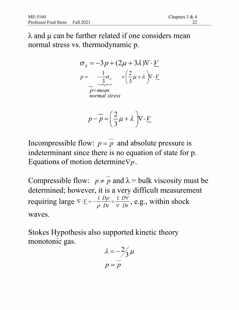
ME:5160 Chapters 3 & 4 Professor Fred Stern Fall 2021 31
Reconsider the problem for fully developed flow: Continuity:
0in out
in out
m mm m m− + =
= =
or Q = constant
Momentum:
( ) ( )21 2
2 2
( )
( ) ( )( )
0
xin out
ave in ave out
ave out in
F p p R F u V n dA u V n dA
AV AVQV
π ρ ρ
ρ β ρ βρ β β
= − − = ⋅ + ⋅
= − += −=
∑ ∫ ∫
(𝑝𝑝1 − 𝑝𝑝2)𝜋𝜋𝑅𝑅2 − 𝜏𝜏𝑓𝑓2𝜋𝜋𝑅𝑅dx = 0
Δ𝑝𝑝𝜋𝜋𝑅𝑅2 − 𝜏𝜏𝑓𝑓2𝜋𝜋𝑅𝑅dx = 0 Since Δ𝑝𝑝 = 𝑝𝑝1 − 𝑝𝑝2 = −𝑑𝑑𝑝𝑝 = −(𝑝𝑝2 − 𝑝𝑝1)
−=
dxdpR
w 2τ or for smaller CV r < R,
−=
dxdpr
2τ
(valid for laminar or turbulent flow, but assume laminar)
0dpdx
< favorable pressure gradient, i.e., Δ𝑝𝑝 = 𝑝𝑝1 − 𝑝𝑝2 = −𝑑𝑑𝑝𝑝 > 0
0dpdx
> adverse pressure gradient, i.e., Δ𝑝𝑝 = 𝑝𝑝1 − 𝑝𝑝2 = −𝑑𝑑𝑝𝑝 < 0

ME:5160 Chapters 3 & 4 Professor Fred Stern Fall 2021 32
−=−==
dxdpr
drdu
dydu
2µµτ y = R-r (wall coordinate)
−−=
dxdpr
drdu
µ2
cdxdpru +
−−=
µ4
2
0)( == Rru
−=
dxdpRc
µ4
2
−
−=
dxdprRru
µ4)(
22
(If 𝑑𝑑𝑝𝑝𝑑𝑑𝑥𝑥
< 0 flow moves from left to right)
−=
dxdpRu
µ4
2
max
−=
2
2
max 1)(Rruru
−=∫=
dxdpRdrrruQ
R
µππ8
2)(4
0
2
max28ave
Q R dp uVA dxµ
= = − =
2
8 42 2
ave avew
V VR dp Rdx R R
µ µτ = − = =

ME:5160 Chapters 3 & 4 Professor Fred Stern Fall 2021 33
2
8 32 64 64Re
w
ave ave ave
fV RV V Dτ µ µ
ρ ρ ρ= = = =
Re aveV Dν
= Exact solution NS for laminar fully developed pipe flow! Piezometric head
h = z +p𝛾𝛾
For a horizontal pipe ∆𝑝𝑝 = 𝛾𝛾∆ℎ , ∆𝜕𝜕 = 0
2 𝑑𝑑𝑥𝑥 𝜏𝜏𝑤𝑤
𝑅𝑅= −𝑑𝑑𝑝𝑝 = ∆𝑝𝑝 = 2 𝐿𝐿 𝜏𝜏𝑤𝑤
𝑅𝑅 , 𝑓𝑓 = 8𝜏𝜏𝑤𝑤
𝜌𝜌𝐶𝐶𝑎𝑎𝑎𝑎2
∆𝑝𝑝 = 2𝐿𝐿𝜌𝜌𝐶𝐶𝑎𝑎𝑎𝑎2 𝑓𝑓
8𝑅𝑅= 𝐿𝐿𝜌𝜌𝐶𝐶𝑎𝑎𝑎𝑎2 𝑓𝑓
2𝐷𝐷
Dividing by 𝛾𝛾 ∆𝑝𝑝𝛾𝛾
=𝐿𝐿𝜌𝜌𝑉𝑉𝑟𝑟𝑣𝑣2 𝑓𝑓
2𝐷𝐷𝛾𝛾= 𝑓𝑓
𝐿𝐿𝐷𝐷𝑉𝑉𝑟𝑟𝑣𝑣2
2𝑔𝑔
More generally
∆ℎ = 𝑓𝑓 𝐿𝐿𝐷𝐷𝐶𝐶𝑎𝑎𝑎𝑎2
2𝑎𝑎 Darcy–Weisbach equation

ME:5160 Chapters 3 & 4 Professor Fred Stern Fall 2021 34
Application of relative inertial coordinates for a moving but non-deforming control volume (CV) The CV moves at a constant velocity CSV with respect to the absolute inertial coordinates. If RV represents the velocity in the relative inertial coordinates that move together with the CV, then: R CSV V V= − Reynolds transport theorem for an arbitrary moving deforming CV:
SYS
RCV CS
dB d d V n dAdt dt
βρ βρ= ∀ + ⋅∫ ∫
For a non-deforming CV moving at constant velocity, RTT for incompressible flow:
syst
RCV CS
dBd V ndA
dt tβρ ρ β∂
= ∀ + ⋅∂∫ ∫
1. Conservation of mass systB M= , and 1β = :
dAnVddtd
dtdM
CSR
CV∫∫ ⋅+∀== ρρ0
dAnVddtd
CSR
CV∫∫ ⋅=∀− ρρ
For steady flow and ρ=constant: 0R
CS
V ndA⋅ =∫
ME:5160 Chapters 3 & 4 Professor Fred Stern Fall 2021 35 2. Conservation of momentum
( )CSsyst RB M V V= + and syst R CSdB dM V V Vβ = = + =
( ) ( ) ( )[ ]CS CSR R
CSR RCV CS
d M V V V VF d V V V ndA
dt tρ ρ
+ ∂ += = ∀ + + ⋅
∂∑ ∫ ∫
For steady flow with the use of continuity:
( )CSR RCS
CSR R RCS CS
F V V V ndA
V V ndA V V ndA
ρ
ρ ρ
= + ⋅
= ⋅ + ⋅
∑ ∫
∫ ∫0
(since CSV = constant and using continuity)
R RCS
F V V ndAρ= ⋅∑ ∫

ME:5160 Chapters 3 & 4 Professor Fred Stern Fall 2021 36
Example (use relative inertial coordinates): A jet strikes a vane which moves to the right at constant velocity 𝑉𝑉𝐶𝐶 on a
frictionless cart. Compute (a) the force 𝐹𝐹𝑥𝑥 required to restrain the cart and (b) the power 𝑃𝑃 delivered to the cart. Also find the cart velocity for which (c) the force 𝐹𝐹𝑥𝑥 is a maximum and (d) the power 𝑃𝑃 is a maximum.
Solution:
Assume relative inertial coordinates with non-deforming CV i.e. CV moves
at constant translational non-accelerating 𝑉𝑉𝐶𝐶𝑆𝑆 = 𝑢𝑢𝐶𝐶𝑆𝑆𝚤𝚤 + 𝑣𝑣𝐶𝐶𝑆𝑆𝚥𝚥 + 𝑤𝑤𝐶𝐶𝑆𝑆𝑘𝑘 = 𝑉𝑉𝐶𝐶𝚤𝚤 then R CSV V V= − . Also assume steady flow 𝑉𝑉 ≠ 𝑉𝑉(𝑑𝑑) with 𝜌𝜌 = 𝑐𝑐𝑐𝑐𝑛𝑛𝑐𝑐𝑑𝑑𝑐𝑐𝑛𝑛𝑑𝑑 and neglect gravity effect. Continuity: 0 = 𝜌𝜌 ∫ 𝑉𝑉𝑅𝑅 ⋅ 𝑛𝑛𝑑𝑑𝑑𝑑𝐶𝐶𝑆𝑆
−𝜌𝜌𝑉𝑉𝑅𝑅1𝑑𝑑1 + 𝜌𝜌𝑉𝑉𝑅𝑅2𝑑𝑑2 = 0 𝑉𝑉𝑅𝑅1𝑑𝑑1 = 𝑉𝑉𝑅𝑅2𝑑𝑑2 = 𝑉𝑉𝑖𝑖 − 𝑉𝑉𝐶𝐶
𝐶𝐶𝑅𝑅1=𝐶𝐶𝑅𝑅𝑥𝑥1=𝐶𝐶𝑗𝑗−𝐶𝐶𝐶𝐶
𝑑𝑑𝑖𝑖
Bernoulli without gravity:
1p0 2
1 212 RV pρ+ =
0 22
12 RVρ+
1 2R RV V=

ME:5160 Chapters 3 & 4 Professor Fred Stern Fall 2021 37
1 2 jA A A= = Momentum:
∑𝐹𝐹 = 𝜌𝜌 𝑉𝑉𝑅𝑅 𝑉𝑉𝑅𝑅 ⋅ 𝑛𝑛𝑑𝑑𝑑𝑑𝐶𝐶𝑆𝑆
x x Rx RCSF F V V ndAρ= − = ⋅∑ ∫
−𝐹𝐹𝑥𝑥 = 𝜌𝜌𝑉𝑉𝑅𝑅𝑥𝑥1(−𝑉𝑉𝑅𝑅1𝑑𝑑1) + 𝜌𝜌𝑉𝑉𝑅𝑅𝑥𝑥2(𝑉𝑉𝑅𝑅2𝑑𝑑2)
−𝐹𝐹𝑥𝑥 = 𝜌𝜌𝑉𝑉𝑖𝑖 − 𝑉𝑉𝐶𝐶−𝑉𝑉𝑖𝑖 − 𝑉𝑉𝐶𝐶𝑑𝑑𝑖𝑖 + 𝜌𝜌𝑉𝑉𝑖𝑖 − 𝑉𝑉𝐶𝐶 cos𝜃𝜃 𝑉𝑉𝑖𝑖 − 𝑉𝑉𝐶𝐶𝑑𝑑𝑖𝑖
𝐹𝐹𝑥𝑥 = 𝜌𝜌𝑉𝑉𝑖𝑖 − 𝑉𝑉𝐶𝐶
2𝑑𝑑𝑖𝑖[1 − cos 𝜃𝜃]
𝑃𝑃𝑐𝑐𝑤𝑤𝑃𝑃𝑃𝑃 = 𝑉𝑉𝐶𝐶𝐹𝐹𝑥𝑥 = 𝑉𝑉𝐶𝐶𝜌𝜌𝑉𝑉𝑖𝑖 − 𝑉𝑉𝐶𝐶2𝑑𝑑𝑖𝑖(1 − cos𝜃𝜃)
𝐹𝐹𝑥𝑥𝑖𝑖𝑟𝑟𝑥𝑥 = 𝜌𝜌𝑉𝑉𝑖𝑖2𝑑𝑑𝑖𝑖(1 − cos𝜃𝜃), 𝑉𝑉𝐶𝐶 = 0
𝑃𝑃𝑖𝑖𝑟𝑟𝑥𝑥 ⇒
𝑑𝑑𝑃𝑃𝑑𝑑𝑉𝑉𝐶𝐶
= 0
𝑃𝑃 = 𝑉𝑉𝐶𝐶𝜌𝜌𝑉𝑉𝑖𝑖2 − 2𝑉𝑉𝐶𝐶𝑉𝑉𝑖𝑖 + 𝑉𝑉𝐶𝐶2𝑑𝑑𝑖𝑖(1 − cos𝜃𝜃) = 𝜌𝜌𝑉𝑉𝑖𝑖2𝑉𝑉𝐶𝐶 − 2𝑉𝑉𝐶𝐶2𝑉𝑉𝑖𝑖 + 𝑉𝑉𝐶𝐶3𝑑𝑑𝑖𝑖(1 − cos𝜃𝜃)
𝑑𝑑𝑃𝑃𝑑𝑑𝑉𝑉𝐶𝐶
= 𝜌𝜌𝑉𝑉𝑖𝑖2 − 4𝑉𝑉𝐶𝐶𝑉𝑉𝑖𝑖 + 3𝑉𝑉𝐶𝐶2𝑑𝑑𝑖𝑖(1 − cos𝜃𝜃) = 0
3𝑉𝑉𝐶𝐶2 − 4𝑉𝑉𝑖𝑖𝑉𝑉𝐶𝐶 + 𝑉𝑉𝑖𝑖2 = 0
𝑉𝑉𝐶𝐶 =+4𝑉𝑉𝑖𝑖 ± 16𝑉𝑉𝑖𝑖2 − 12𝑉𝑉𝑖𝑖2
6=
4𝑉𝑉𝑖𝑖 ± 2𝑉𝑉𝑖𝑖6
For 3j
C
VV = : 𝑃𝑃𝑖𝑖𝑟𝑟𝑥𝑥 =
𝐶𝐶𝑗𝑗3𝜌𝜌
2𝐶𝐶𝑗𝑗32𝑑𝑑𝑖𝑖(1 − cos𝜃𝜃) = 4
27𝑉𝑉𝑖𝑖3𝜌𝜌𝑑𝑑𝑖𝑖(1 − cos𝜃𝜃)

ME:5160 Chapters 3 & 4 Professor Fred Stern Fall 2021 38
Example (use absolute inertial and relative inertial coordinates)
Assume gravity force is negligible and the cross section area of the jet does not change after striking the bucket. Taking moving CV at speed Vs= ΩR î enclosing jet and bucket: Solution 1 (relative inertial coordinates) Continuity: , , 0in R out Rm m− + =
, , RR in R out RCS
m m m V n dAρ= = = ⋅∫
Bernoulli without gravity:
ΩR
CV
Vout,R
Vin,R

ME:5160 Chapters 3 & 4 Professor Fred Stern Fall 2021 39
1p0 2
, 212 in RV pρ+ =
0 2,
12 out RVρ+
, ,in R out RV V=
Inlet 𝑉𝑉𝑖𝑖𝚤𝚤,𝑅𝑅 = 𝑉𝑉𝑖𝑖 − 𝛺𝛺𝑅𝑅𝚤𝚤 Outlet 𝑉𝑉𝑜𝑜𝑜𝑜𝑜𝑜,𝑅𝑅 = −𝑉𝑉𝑖𝑖 − 𝛺𝛺𝑅𝑅𝚤𝚤 Since , 1 , 2 0in R out RV A V Aρ ρ− + = 1 2 jA A A= =
Momentum: , ,X bucket R out R R in RF F m V m V= − = −∑
2
( ) ( )
2 ( )
2 ( )
bucket R j j
R j
j j
F m V R V R
m V R
A V Rρ
= − − − Ω − − Ω = − Ω
= − Ω
( )R j jm A V Rρ= − Ω 22 ( )bucket j jP RF A R V Rρ= Ω = Ω − Ω
𝑑𝑑𝑃𝑃𝑑𝑑𝛺𝛺
= 2𝜌𝜌𝑑𝑑𝑖𝑖𝑅𝑅𝑉𝑉𝑖𝑖 − 𝛺𝛺𝑅𝑅2 − 2𝜌𝜌𝑑𝑑𝑖𝑖𝛺𝛺𝑅𝑅2𝑉𝑉𝑖𝑖 − 𝛺𝛺𝑅𝑅𝑅𝑅
= 2𝜌𝜌𝑑𝑑𝑖𝑖𝑅𝑅 𝑉𝑉𝑖𝑖 − 𝛺𝛺𝑅𝑅2 − 2𝑅𝑅𝛺𝛺𝑉𝑉𝑖𝑖 − 𝛺𝛺𝑅𝑅 = 2𝜌𝜌𝑑𝑑𝑖𝑖𝑅𝑅𝑉𝑉𝑖𝑖 − 𝛺𝛺𝑅𝑅𝑉𝑉𝑖𝑖 − 𝛺𝛺𝑅𝑅 − 2𝑅𝑅𝛺𝛺
𝑑𝑑𝑃𝑃𝑑𝑑𝛺𝛺
= 0 → 𝑉𝑉𝑖𝑖 − 3𝛺𝛺𝑅𝑅 = 0 → 𝑉𝑉𝑖𝑖3
= 𝛺𝛺𝑅𝑅
𝑃𝑃𝑖𝑖𝑟𝑟𝑥𝑥 = 2𝜌𝜌𝑑𝑑𝑖𝑖𝑉𝑉𝑖𝑖3𝑉𝑉𝑖𝑖 −
𝑉𝑉𝑖𝑖32
= 2𝜌𝜌𝑑𝑑𝑖𝑖𝑉𝑉𝑖𝑖3
4𝑉𝑉𝑖𝑖2
9=
8270.296
𝜌𝜌𝑑𝑑𝑖𝑖𝑉𝑉𝑖𝑖3

ME:5160 Chapters 3 & 4 Professor Fred Stern Fall 2021 40
If infinite number of buckets: R j jm A Vρ=
3max
2 ( )
2 ( )
102 2
bucket j j j
j j j
jj j
F A V V R
P A V R V R
VdP for R P A Vd
ρ
ρ
ρ
= − Ω
= Ω − Ω
= Ω = =Ω
Solution 2 (absolute inertial coordinates)
𝑉𝑉𝑅𝑅 = 𝑉𝑉 − 𝑉𝑉𝐶𝐶𝑆𝑆 → 𝑉𝑉 = 𝑉𝑉𝑅𝑅 + 𝑉𝑉𝐶𝐶𝑆𝑆
𝑉𝑉𝑖𝑖𝚤𝚤 = 𝑉𝑉𝑖𝑖 𝚤𝚤
𝑉𝑉𝑜𝑜𝑜𝑜𝑜𝑜 = −𝑉𝑉𝑖𝑖 − 𝛺𝛺𝑅𝑅 𝚤𝚤 + 𝛺𝛺𝑅𝑅 𝚤𝚤 = −𝑉𝑉𝑖𝑖 − 2𝛺𝛺𝑅𝑅 𝚤𝚤 Continuity: from solution 1
−𝑉𝑉𝑖𝑖𝚤𝚤,𝑅𝑅 + 𝑉𝑉𝑜𝑜𝑜𝑜𝑜𝑜,𝑅𝑅 = 0 express in the absolute inertial coordinates: 𝑉𝑉𝑅𝑅 = 𝑉𝑉 − 𝑉𝑉𝐶𝐶𝑆𝑆
−𝑉𝑉𝑖𝑖 − 𝛺𝛺𝑅𝑅 𝚤𝚤 + 𝑉𝑉𝑖𝑖 + 2𝛺𝛺𝑅𝑅 − 𝛺𝛺𝑅𝑅 𝚤𝚤 = 0
all jet mass flow result in work.

ME:5160 Chapters 3 & 4 Professor Fred Stern Fall 2021 41
Momentum:
𝐹𝐹𝑥𝑥 = −𝐹𝐹𝑏𝑏𝑜𝑜𝑓𝑓𝑏𝑏𝑛𝑛𝑜𝑜 = 𝑚(𝑉𝑉𝑜𝑜𝑜𝑜𝑜𝑜 − 𝑉𝑉𝑖𝑖𝚤𝚤)
= 𝜌𝜌𝑑𝑑𝑖𝑖𝑉𝑉𝑖𝑖 − 𝛺𝛺𝑅𝑅−𝑉𝑉𝑖𝑖 − 2𝛺𝛺𝑅𝑅 − 𝑉𝑉𝑖𝑖
𝐹𝐹𝑏𝑏𝑜𝑜𝑓𝑓𝑏𝑏𝑛𝑛𝑜𝑜 = 2𝜌𝜌𝑑𝑑𝑖𝑖𝑉𝑉𝑖𝑖 − 𝛺𝛺𝑅𝑅2 Same as Solution 1.

ME:5160 Chapters 3 & 4 Professor Fred Stern Fall 2021 42
Application of CV continuity equation for steady incompressible flow, fixed CV, one inlet and outlet with A = constant
in out
V ndA V ndA m Qρ ρ ρ⋅ = ⋅ = =∫ ∫
in outQ Q= ( ) ( )ave avein outV A V A=
For A = constant ( ) ( )ave avein outV V= ( ) ( )
in out
F V V n dA V V n dAρ ρ= ⋅ + ⋅∑ ∫ ∫
Pipe: ( ) ( )x
in out
F u V n dA u V n dAρ ρ= ⋅ + ⋅∑ ∫ ∫
( ) ( )2 2ave avein out
AV AVρ β ρ β= − + ( )ave out inQVρ β β= − change in shape u
Vane: 𝐹𝐹 = 𝑚 𝑉𝑉𝑜𝑜𝑜𝑜𝑜𝑜 − 𝑉𝑉𝑖𝑖𝚤𝚤 ; |𝑉𝑉𝑜𝑜𝑜𝑜𝑜𝑜| = |𝑉𝑉𝑖𝑖𝚤𝚤|
If θ=180: ( ) ( )2x out in inF m u u m u= − = −∑
For arbitrary θ:
𝐹𝐹𝑥𝑥 = 𝑚(𝑢𝑢𝑜𝑜𝑜𝑜𝑜𝑜 cos𝜃𝜃 − 𝑢𝑢𝑖𝑖𝚤𝚤) = 𝑚𝑢𝑢𝑖𝑖𝚤𝚤(cos𝜃𝜃 − 1) change in direction u

ME:5160 Chapters 3 & 4 Professor Fred Stern Fall 2021 43
Application of differential momentum equation:
1. NS valid both laminar and turbulent flow; however, many orders of magnitude difference in temporal and spatial resolution, i.e., turbulent flow requires very small time and spatial scales
2. Laminar flow Recrit = Uδν
≤ about 2000 Re > Recrit instability
3. Turbulent flow Retransition > 10 or 20 Recrit
Random motion superimposed on mean coherent structures. Cascade: energy from large scale dissipates at smallest scales due to viscosity. Kolmogorov hypothesis for smallest scales
4. No exact solutions for turbulent flow: RANS, DES,
LES, DNS (all CFD)

ME:5160 Chapters 3 & 4 Professor Fred Stern Fall 2021 44
5. 80 exact solutions for simple laminar flows are mostly linear 0V V⋅∇ = . Topics of exact analytical solutions:
I. Couette (wall/shear-driven) steady flows a. Channel flows b. Cylindrical flows
II. Poiseuille (pressure-driven) steady flows a. Channel flows b. Duct flows
III. Combined Couette and Poiseuille steady flows IV. Gravity and free-surface steady flows V. Unsteady flows
VI. Suction and injection flows VII. Wind-driven (Ekman) flows
VIII. Similarity solutions
6. Also, many exact solutions for low Re linearized creeping motion Stokes flows and high Re nonlinear BL approximations.
7. Can also use CFD for non-simple laminar flows 8. AFD or CFD requires well posed IBVP; therefore,
exact solutions are useful for setup of IBVP, physics, and verification CFD since modeling errors yield USM = 0 and only errors are numerical errors USN, i.e., assume analytical solution = truth, called analytical benchmark.

ME:5160 Chapters 3 & 4 Professor Fred Stern Fall 2021 45
Energy Equation: B = E = energy β = e = dE/dm = energy per unit mass Integral Form (fixed CV):
( )
CV CS
dE e d e V n dA Q Wdt t
rateof change rateof outfluxE in CV E across CS
ρ ρ∂= ∀ + ⋅ = −
∂∫ ∫
=++= gzvue 2
21^
internal + KE + PE
Q = conduction + convection + radiation
/shaft pW W W W
pressure viscouspump turbineν= + +
( )pdW p ndA V= ⋅ - pressure force × velocity
( )pCS
W p V n dA= ⋅∫
Rate of change E
Rate of heat added CV
Rate work done by CV

ME:5160 Chapters 3 & 4 Professor Fred Stern Fall 2021 46
vdW dA Vτ= − ⋅
- viscous force × velocity
vCS
W V dAτ= − ⋅∫
( )( ) /sCV CS
Q W W e d e p V n dAtν ρ ρ ρ∂
− − = ∀ + + ⋅∂∫ ∫
For our purposes, we are interested in steady flow one inlet and outlet. Also 𝑊𝑣𝑣 ≈ 0 in most cases; since, V = 0 at solid surface; on inlet and outlet only τn ~ 0 since its perpendicular to flow; or for V ≠ 0 and τstreamline ~ 0 if outside BL.
2
&
1ˆ /2S
inlet outlet
Q W u V gz p V n dAρ ρ − = + + + ⋅ ∫
Assume parallel flow with /p gzρ +
and u constant over
inlet and outlet.
( ) 2
& &
ˆ / ( )2S
inlet outlet inlet outlet
Q W u p gz V n dA V V n dAρρ ρ− = + + ⋅ + ⋅∫ ∫
( ) 3ˆ / ( )
2S in in ininin
Q W u p gz m V dAρρ− = + + − − ∫
( ) 3ˆ / ( )2out out outout
out
u p gz m V dAρρ+ + + + ∫
= constant i.e., hydrostatic pressure variation

ME:5160 Chapters 3 & 4 Professor Fred Stern Fall 2021 47
Define kinetic energy correction factor
3 221 ( )
2 2ave
aveA A
VV dA V V n dA mA V
ρα α•
= → ⋅ =
∫ ∫
Laminar flow:
−=
2
0 1RrUu
Vave=0.5 β = 4/3 α=2
Turbulent flow: m
RrUu
−= 10
( ) ( )3 31 24(1 3 )(2 3 )
m mm m
α+ +
=+ +
m=1/7 α=1.058 as with β, α~1 for
turbulent flow
2 2
ˆ ˆ( / ) ( / )2 2
s ave aveout in
W V VQ u p gz u p gzm m
ρ α ρ α− = + + + − + + +
Let in = 1, out = 2, V = Vave, and divide by g
2 21 1 2 21 1 2 22 2p t L
p pV z h V z h hg g g g
α αρ ρ
+ + + = + + + +

ME:5160 Chapters 3 & 4 Professor Fred Stern Fall 2021 48
ps tt p
WW W h hgm gm gm
= − = −
Where ht extracts and hp adds energy
2 11 ( )L
Qh u ug mg
= − −
hL = thermal energy (other terms represent mechanical energy
1 1 2 2m AV A Vρ ρ= = Assuming no heat transfer mechanical energy converted to thermal energy through viscosity and cannot be recovered; therefore, it is referred to as head loss > 0, which can be shown from 2nd law of thermodynamics. 1D energy equation can be considered as modified Bernoulli equation for hp, ht, and hL.

ME:5160 Chapters 3 & 4 Professor Fred Stern Fall 2021 49
Application of 1D Energy equation fully developed pipe flow without hp or ht. Recall the horizontal pipe flow using continuity and momentum: 𝜏𝜏𝑓𝑓 = 𝑅𝑅
2− 𝑑𝑑𝑝𝑝
𝑑𝑑𝑥𝑥, i.e., −𝑑𝑑𝑝𝑝
𝑑𝑑𝑥𝑥= 2𝜏𝜏𝑤𝑤
𝑅𝑅
Similarly, for non-horizontal pipe: − 𝑑𝑑
𝑑𝑑𝑥𝑥(𝑝𝑝 + 𝛾𝛾𝜕𝜕) = 2𝜏𝜏𝑤𝑤
𝑅𝑅
Using energy equation, 𝐿𝐿 = 𝑑𝑑𝜕𝜕 and 𝑝 = 𝑝𝑝 + 𝛾𝛾𝜕𝜕: ℎ𝐿𝐿 = 𝑝𝑝1−𝑝𝑝2
𝜌𝜌𝑎𝑎+ (𝜕𝜕1 − 𝜕𝜕2) = 𝐿𝐿
𝜌𝜌𝑎𝑎− 𝑑𝑑
𝑑𝑑𝑥𝑥(𝑝𝑝 + 𝛾𝛾𝜕𝜕)
ℎ𝐿𝐿 = 𝐿𝐿
𝜌𝜌𝑎𝑎− 𝑑𝑑𝑝𝑝
𝑑𝑑𝑥𝑥 = 𝐿𝐿
𝜌𝜌𝑎𝑎2𝜏𝜏𝑤𝑤
𝑅𝑅 (If 𝑑𝑑𝑝𝑝
𝑑𝑑𝑥𝑥< 0 flow moves from left to right)
Where 𝜏𝜏𝑓𝑓 = 1
8𝑓𝑓𝜌𝜌𝑉𝑉𝑟𝑟𝑣𝑣𝑛𝑛2
ℎ𝐿𝐿 = ℎ𝑓𝑓 = 𝑓𝑓𝐿𝐿𝐷𝐷𝑉𝑉𝑟𝑟𝑣𝑣𝑛𝑛2
2𝑔𝑔
Where ℎ𝑓𝑓 is the friction loss Also recall for laminar flow that 𝜏𝜏𝑓𝑓 = 4𝜇𝜇𝐶𝐶𝑎𝑎𝑎𝑎𝑎𝑎
𝑅𝑅
2
8 32 64 / Re
Re /
wD
ave ave
D ave
fV RVV D
τ µρ ρ
ν
= = =
=
2
32 aveL
LVhD
µγ
= ∝ Vave exact solution!
Darcy-Weisbach Equation (valid for laminar or Turbulent

ME:5160 Chapters 3 & 4 Professor Fred Stern Fall 2021 50
Note: Po = Poiseuille number = fRe = 64 = pure constant, which is the case for all laminar flows regardless duct cross section but with different constant depending on cross section; since, τw∝Vave For turbulent flow, Recrit ~ 2000, Retrans ~ 3000 f=f (Re, k/D) Re = VaveD/ν, k = roughness τw and 2
L aveh V∝ Pipe with minor losses,
hL = hf + Σhm where
2
2mVh K
gK loss coefficient
=
=
hm = “so called” minor losses, e.g., entrance/exit, expansion/contraction, bends, elbows, tees, other fitting, and valves.

ME:5160 Chapters 3 & 4 Professor Fred Stern Fall 2021 51
(a) First suppose 2D problem: D1 and D2 denotes width in y instead of diameter and we take unit in z (span-wise) direction
22 2
2
.79 989 0.02 1 425xF F mV V NAρ
= − = − ⇒ ∗ × × × =∑
2 5.22 / , 81.6 /V m s m kg s= = Continuity equation between points 1 and 2
2
1 1 2 2 1 21
2.09 /DV A V A V V m sD
= ⇒ = =
Bernoulli neglect g, p2=pa 2 2
1 1 2 21 12 2
p V p Vρ ρ+ = + hL=0, z=constant
( )2 21 2 2 1
12
p p V Vρ= + − 2 21
.79 998101,000 (5.22 2.09 )2
p ×= + −
1 110,020p Pa=
Note: 2 2 22 2 3 3 4 42 2 2
p V p V p Vρ ρ ρ+ = + = +
2 3 4 2 3 4ap p p p V V V= = = → = =

ME:5160 Chapters 3 & 4 Professor Fred Stern Fall 2021 52
2 2 3 3 4 40CS
V A A V A V A Vρ= ⋅ → = +∑ 432 AAA += 3 3 3 4 4 40 ( )y
CSF VV A V V A V V Aρ ρ ρ= = ⋅ = + −∑ ∑
2 23 3 4 4V A V Aρ ρ= − 43 AA =
(b) For the round jet implied in the problem statement
2 2
2 2
2
.79 989 .02 4254xF F mV V N
A
π
ρ= − = − ⇒ ∗ =∑
2 41.4 / , 10.3 /V m s m kg s•
= = Continuity equation between points 1 and 2
2
21 1 2 2 1 2
1
DV A V A V VD
= ⇒ =
2
1241.45
V = 1 6.63 /V m s=
Bernoulli neglect g, p2=pa
2 21 1 2 2
1 12 2
p V p Vρ ρ+ = + hL=0, z=constant
( )2 21 2 2 1
12
p p V Vρ= + − 2 21
.79 998101,000 (41.4 6.63 )2
p ×= + −
Pap 000,7601 =

ME:5160 Chapters 3 & 4 Professor Fred Stern Fall 2021 53
(a)
22
1 22Vz z
g= + 0,11,0,1 212 ==== zzhLα
2 1 22 ( )V g z z= − 11*81.9*2= sm /7.14=
2 32 2 2 (.01) *14.7*3600 4.16 /
4Q A V m hπ
= = =
56
14.7 0.01Re 1.5 1010
VDν −
×= = = ×
(b) 2
21 2 22 L
Vz z hg
α= + + 6 2
2 2
322, , 10 /LVLh m s
D gµα ν
ρ−= = =
22 23.2 107.8 0V V+ − =
V2 = 8.9 m/s Q= 2.516 m3/h
Re=89,000=8.9*104 >>2000
Torricelli’s expression for speed of efflux from reservoir

ME:5160 Chapters 3 & 4 Professor Fred Stern Fall 2021 54
(c)
2 22 2
1 2 22 2V VLz z f
g D gα= + +
α2=1
( )2
21 2 1 /
2Vz z fL D
g− = +
[ ]12
2 1 22 ( ) /(1 / )V g z z fL D= − +
[ ]12
2 216 /(1 *1000)V f= + (Re), Re VDf fν
= = guess f = 0.015 (smooth pipe Moody diagram)
42
42
42
3.7 / Re 3.7 10 , .0242.94 / Re 2.9 10 , .0252.88 / Re 2.9 10
V m s x fV m s x fV m s x
= → = =
= → = =
= → =
(d) Re 2000VDν
= = 2000D
Vν
=
2
2 21 2 2 2 2
22
32( )20002
V LVz zg g
V
ναν
− = +
2 3
2 21 2 2 2
32( )2 2000V LVz z
g gνα
ν− = +
3 2
2 22
32 11 02000
LV Vg gν
+ − = 2 1.1 /V m s= mD 00182.0=
Low U and small D to actually have laminar flow

ME:5160 Chapters 3 & 4 Professor Fred Stern Fall 2021 55
Differential Form of Energy Equation:
( ) ( )CV
dE e e V d Q Wdt t
ρ ρ
∂ = + ∇ ⋅ ∀ = − ∂ ∫
𝜌𝜌𝜕𝜕𝑃𝑃𝜕𝜕𝑑𝑑
+ 𝑃𝑃𝜕𝜕𝜌𝜌𝜕𝜕𝑑𝑑
+ 𝑃𝑃∇. 𝜌𝜌𝑉𝑉=0
+ 𝜌𝜌𝑉𝑉.∇𝑃𝑃 = 𝜌𝜌𝐷𝐷𝑃𝑃𝐷𝐷𝑑𝑑
= 𝜌𝜌 𝜕𝜕𝑃𝑃𝜕𝜕𝑑𝑑
+ 𝑉𝑉.∇𝑃𝑃
2 21 1ˆ ˆ2 2
e u V gz u V g r= + + = + − ⋅ ˆ
( ) /De Du DVQ W q w V g VDt Dt Dt
ρ ρ = − ∀ = − = + − ⋅
( )q q k T= −∇ ⋅ = ∇ ⋅ ∇ Fourier’s Law
𝑤 = −∇ ⋅ 𝑉𝑉 ⋅ 𝜎𝜎𝑖𝑖𝑖𝑖 = −𝑉𝑉 ⋅ ∇ ⋅ 𝜎𝜎𝑖𝑖𝑖𝑖𝜌𝜌𝐷𝐷𝐶𝐶𝐷𝐷𝑜𝑜−𝑎𝑎
𝑖𝑖𝑜𝑜𝑖𝑖𝑛𝑛𝚤𝚤𝑜𝑜𝑜𝑜𝑖𝑖𝑛𝑛𝑒𝑒𝑜𝑜𝑟𝑟𝑜𝑜𝑖𝑖𝑜𝑜𝚤𝚤
− 𝜎𝜎𝑖𝑖𝑖𝑖𝜕𝜕𝑢𝑢𝑖𝑖𝜕𝜕𝜕𝜕𝑖𝑖
First term for 𝑤 −𝑉𝑉 ⋅ ∇ ⋅ 𝜎𝜎𝑖𝑖𝑖𝑖 = −𝑉𝑉 ⋅ 𝜌𝜌
𝐷𝐷𝑉𝑉𝐷𝐷𝑑𝑑
− 𝑔𝑔 = −𝜌𝜌 𝑉𝑉 ⋅𝐷𝐷𝑉𝑉𝐷𝐷𝑑𝑑
− 𝑉𝑉 ⋅ 𝑔𝑔
Where
𝑉𝑉 ⋅𝐷𝐷𝑉𝑉𝐷𝐷𝑑𝑑
= 𝑉𝑉 ⋅ 𝜕𝜕𝑉𝑉𝜕𝜕𝑑𝑑
+ 𝑉𝑉 ⋅ ∇𝑉𝑉 =𝜕𝜕𝑉𝑉2
𝜕𝜕𝑑𝑑+ 𝑉𝑉 ⋅ ∇𝑉𝑉2 = 𝑉𝑉
𝐷𝐷𝑉𝑉𝐷𝐷𝑑𝑑
Therefore −𝑉𝑉 ⋅ ∇ ⋅ 𝜎𝜎𝑖𝑖𝑖𝑖 = −𝜌𝜌 𝑉𝑉
𝐷𝐷𝑉𝑉𝐷𝐷𝑑𝑑
− 𝑉𝑉 ⋅ 𝑔𝑔

ME:5160 Chapters 3 & 4 Professor Fred Stern Fall 2021 56 And
𝑤 = −𝜌𝜌 𝑉𝑉𝐷𝐷𝑉𝑉𝐷𝐷𝑑𝑑
− 𝑉𝑉 ⋅ 𝑔𝑔 − 𝜎𝜎𝑖𝑖𝑖𝑖𝜕𝜕𝑢𝑢𝑖𝑖𝜕𝜕𝜕𝜕𝑖𝑖
Substitute equation for 𝑞 and 𝑤 𝑞 − 𝑤 = −∇ ⋅ (𝑘𝑘∇T) + 𝜌𝜌 𝑉𝑉
𝐷𝐷𝑉𝑉𝐷𝐷𝑑𝑑
− 𝑉𝑉 ⋅ 𝑔𝑔 + 𝜎𝜎𝑖𝑖𝑖𝑖𝜕𝜕𝑢𝑢𝑖𝑖𝜕𝜕𝜕𝜕𝑖𝑖
= 𝜌𝜌 𝐷𝐷𝑢𝑢𝐷𝐷𝑑𝑑
+ 𝑉𝑉𝐷𝐷𝑉𝑉𝐷𝐷𝑑𝑑
− 𝑉𝑉 ⋅ 𝑔𝑔
𝜌𝜌𝐷𝐷𝑢𝑢𝐷𝐷𝑑𝑑
= −∇ ⋅ (𝑘𝑘∇T)+𝜎𝜎𝑖𝑖𝑖𝑖𝜕𝜕𝑢𝑢𝑖𝑖𝜕𝜕𝜕𝜕𝑖𝑖
Second term on right hand side 𝜎𝜎𝑖𝑖𝑖𝑖
𝜕𝜕𝑢𝑢𝑖𝑖𝜕𝜕𝜕𝜕𝑖𝑖
= (𝜏𝜏𝑖𝑖𝑖𝑖 − 𝑝𝑝𝛿𝛿𝑖𝑖𝑖𝑖)𝜕𝜕𝑢𝑢𝑖𝑖𝜕𝜕𝜕𝜕𝑖𝑖
= 𝜏𝜏𝑖𝑖𝑖𝑖𝜕𝜕𝑢𝑢𝑖𝑖𝜕𝜕𝜕𝜕𝑖𝑖
− 𝑝𝑝∇ ⋅ V
From continuity 𝐷𝐷𝜌𝜌𝐷𝐷𝑑𝑑
+ 𝜌𝜌∇.𝑉𝑉 = 0 → ∇.𝑉𝑉 = −1𝜌𝜌𝐷𝐷𝜌𝜌𝐷𝐷𝑑𝑑
−𝑝𝑝∇.𝑉𝑉 =𝑝𝑝𝜌𝜌𝐷𝐷𝜌𝜌𝐷𝐷𝑑𝑑
= −𝜌𝜌𝐷𝐷𝐷𝐷𝑑𝑑
𝑝𝑝𝜌𝜌 +
𝐷𝐷𝑝𝑝𝐷𝐷𝑑𝑑
Therefore 𝜎𝜎𝑖𝑖𝑖𝑖
𝜕𝜕𝑢𝑢𝑖𝑖𝜕𝜕𝜕𝜕𝑖𝑖
= 𝜏𝜏𝑖𝑖𝑖𝑖𝜕𝜕𝑢𝑢𝑖𝑖𝜕𝜕𝜕𝜕𝑖𝑖
− 𝜌𝜌𝐷𝐷𝐷𝐷𝑑𝑑
𝑝𝑝𝜌𝜌 +
𝐷𝐷𝑝𝑝𝐷𝐷𝑑𝑑
And 𝜌𝜌𝐷𝐷𝑢𝑢𝐷𝐷𝑑𝑑
= −∇ ⋅ (𝑘𝑘∇T) + 𝜏𝜏𝑖𝑖𝑖𝑖𝜕𝜕𝑢𝑢𝑖𝑖𝜕𝜕𝜕𝜕𝑖𝑖
− 𝜌𝜌𝐷𝐷𝐷𝐷𝑑𝑑
𝑝𝑝𝜌𝜌 +
𝐷𝐷𝑝𝑝𝐷𝐷𝑑𝑑
Rearranging equation and substituting dissipation function Φ = 𝜏𝜏𝑖𝑖𝑖𝑖
𝜕𝜕𝑜𝑜𝑖𝑖𝜕𝜕𝑥𝑥𝑗𝑗
≥ 0
𝜌𝜌𝐷𝐷𝐷𝐷𝑑𝑑
u +𝑝𝑝𝜌𝜌 = −∇ ⋅ (𝑘𝑘∇T) +
𝐷𝐷𝑝𝑝𝐷𝐷𝑑𝑑
+ Φ

ME:5160 Chapters 3 & 4 Professor Fred Stern Fall 2021 57
Summary GDE for compressible non-constant property fluid flow
Continuity: ( ) 0Vtρ ρ∂
+ ∇ ⋅ =∂
Momentum: 𝜌𝜌 𝐷𝐷𝐶𝐶
𝐷𝐷𝑜𝑜= 𝜌𝜌𝑔𝑔 − ∇𝑝𝑝 + ∇. 𝜏𝜏𝑖𝑖𝑖𝑖
𝜏𝜏𝑖𝑖𝑖𝑖 = 2𝜇𝜇𝜖𝜖𝑖𝑖𝑖𝑖 + 𝜆𝜆∇.𝑉𝑉𝛿𝛿𝑖𝑖𝑖𝑖
𝑔𝑔 = −𝑔𝑔𝑘𝑘 Energy Φ+∇⋅∇+= )( Tk
DtDp
DtDhρ
Primary variables: p, V, T Auxiliary relations: ρ = ρ (p,T) μ = μ (p,T) (equations of state) h = h (p,T) k = k (p,T) Restrictive Assumptions:
1) Continuum 2) Newtonian fluids 3) Thermodynamic equilibrium 4) 𝑔𝑔 = −𝑔𝑔𝑘𝑘 5) heat conduction follows Fourier’s law 6) no internal heat sources

ME:5160 Chapters 3 & 4 Professor Fred Stern Fall 2021 58
For incompressible constant property fluid flow
ˆ vdu c dT= cv, μ, k, ρ ~ constant
Φ+∇= TkDtDTcv
2ρ
For static fluid or V small
TktTcp
2∇=∂∂ρ heat conduction equation (also valid for solids)
Summary GDE for incompressible constant property fluid flow (cv ~ cp)
0V∇ ⋅ =
2ˆDV gk p VDt
ρ ρ µ= − − ∇ + ∇ “elliptic”
Φ+∇= TkDtDTcp
2ρ where j
iij x
u∂∂
=Φ τ
Continuity and momentum uncoupled from energy; therefore, solve separately and use solution post facto to get T.

ME:5160 Chapters 3 & 4 Professor Fred Stern Fall 2021 59
For compressible flow, ρ solved from continuity equation, T from energy equation, and p = (ρ, T) from equation of state (e.g., ideal gas law). For incompressible flow, ρ = constant and T uncoupled from continuity and momentum equations, the latter of which contains p∇ such that reference p is arbitrary and specified post facto (i.e., for incompressible flow, there is no connection between p and ρ). The connection is between p∇ and 0V∇ ⋅ = , i.e., a solution for p requires 0V∇ ⋅ = .
NS 21 ˆDV p V
Dtν
ρ= − ∇ + ∇ p p zγ= +
)(NS⋅∇ (See derivation details on p.87)
2 21 ji
j i
uuD V pDt x x
νρ
∂∂ − ∇ ∇ ⋅ = − ∇ + ∂ ∂
For 0V∇ ⋅ = :
i
j
j
i
xu
xup
∂∂
∂∂
−=∇ ρ2
Poisson equation determines pressure up to additive constant.

ME:5160 Chapters 3 & 4 Professor Fred Stern Fall 2021 60
Approximate Models: 1) Stokes Flow
For low Re 1, ~ 0UL V Vν
= << ⋅∇ 0V∇ ⋅ =
21V p Vt
νρ
∂= − ∇ + ∇
∂
0)( 2 =∇⇒⋅∇ pNS 2) Boundary Layer Equations For high Re >> 1 and attached boundary layers or fully developed free shear flows (wakes, jets, mixing layers),
v<<U, yx ∂
∂<<
∂∂ , 0=yp , and for free shear flow px = 0.
0=+ yx vu ˆt x y x yyu uu vu p uν+ + = − + non-linear, “parabolic”
0
ˆy
x t x
pp U UU
=
− = +
Many exact solutions; similarity methods
Linear, “elliptic” Most exact solutions NS; and for steady flow superposition, elemental solutions and separation of variables

ME:5160 Chapters 3 & 4 Professor Fred Stern Fall 2021 61
3) Inviscid Flow
( ) 0
, ," "
( ) , , , , ( , )
VtDV g p Euler Equation nonlinear hyperbolicDtDh Dp k T p V T unknowns and h k f p TDt Dt
ρ ρ
ρ ρ
ρ ρ
∂+ ∇ ⋅ =
∂
= − ∇
= + ∇ ⋅ ∇ =
4) Inviscid, Incompressible, Irrotational
∇ × 𝑉𝑉 = 0 → 𝑉𝑉 = ∇𝜑𝜑
∇.𝑉𝑉 = 0 → ∇2𝜑𝜑 = 0 𝑙𝑙𝑙𝑙𝑛𝑛𝑃𝑃𝑐𝑐𝑃𝑃 elliptic ∫ Euler Equation Bernoulli Equation:
2
2p V gz constρ ρ+ + =
Many elegant solutions: Laplace equation using superposition elementary solutions, separation of variables, complex variables for 2D, and Boundary Element methods.

ME:5160 Chapters 3 & 4 Professor Fred Stern Fall 2021 62
Couette Shear Flows: 1-D shear flow between surfaces of like geometry (parallel plates or rotating cylinders). Steady Flow Between Parallel Plates: Combined Couette and Poiseuille Flow.
0
00
x y z
x
Vu v wu
∇ ⋅ =+ + =
=
2ˆDV p VDt
ρ µ= −∇ + ∇ 0=+++∂∂
zyx wuvuuutu
ˆ0 x yyp uµ= − +
Φ+∇= TkDtDTcp
2ρ 0x y zT uT vT wTt
∂+ + + =
∂ 20 yyy ukT µ+=
(note inertia terms vanish identically and ρ is absent from equations)
2 2 2
2 2 2
2
2 2 2
( ) ( ) ( )
( )
x y z
x y y z z x
x y z
y
u v w
v u w v u w
u v w
u
µ
λ
µ
Φ = + ++ + + + + +
+ + +
=

ME:5160 Chapters 3 & 4 Professor Fred Stern Fall 2021 63
Non-dimensional equations, but drop *
Uuu /* = 01
0*
TTTTT
−−
= * /y y h=
0=xu (1) 2
ˆyy xhu p B constUµ
= = − = (2)
[ ]2
01
2
Pr
)( yyy uTTk
UT
Ec
−−
=
µ (3)
B.C. y = 1 u = 1 T = 1 y = -1 u = 0 T = 0 (1) is consistent with 1-D flow assumption. Simple
form of (2) and (3) allow for solution to be obtained by double integration.
21 1(1 ) (1 )
2 2u y B y⇒ = + + −
y=y/h
Solution depends on 2
ˆ xhB pUµ
= − ( ˆ / /xp p x z xγ= ∂ ∂ + ∂ ∂ )
B < 0 ˆ xp is opposite to U B < -0.5 backflow occurs near lower wall |B| >> 1 flow approaches parabolic profile
Linear flow due to U
Parabolic flow due to px Note: linear
superposition since 0V V⋅∇ =
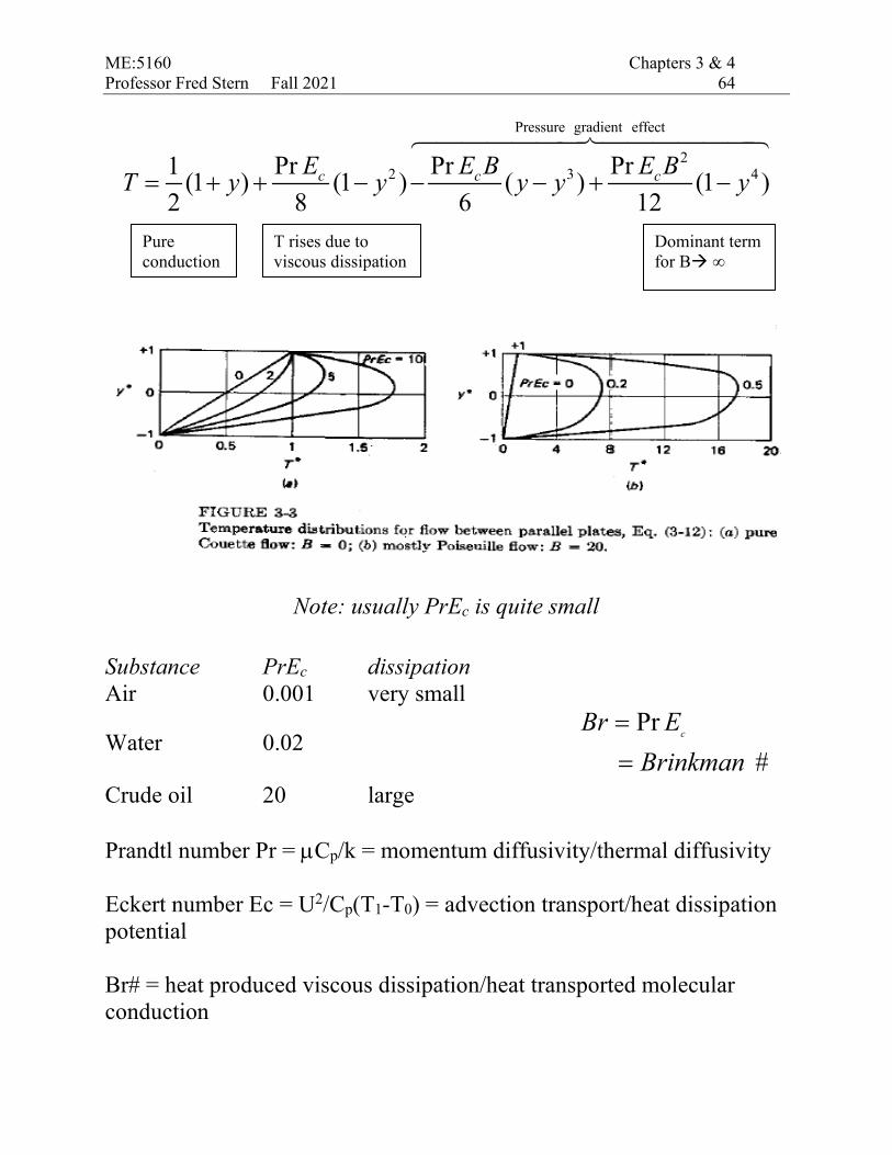
ME:5160 Chapters 3 & 4 Professor Fred Stern Fall 2021 64
Pressure gradient effect
22 3 4Pr Pr Pr1 (1 ) (1 ) ( ) (1 )
2 8 6 12c c cE E B E BT y y y y y= + + − − − + −
Note: usually PrEc is quite small
Substance PrEc dissipation Air 0.001 very small
Water 0.02 #
PrBrinkman
EBr c
==
Crude oil 20 large Prandtl number Pr = µCp/k = momentum diffusivity/thermal diffusivity Eckert number Ec = U2/Cp(T1-T0) = advection transport/heat dissipation potential Br# = heat produced viscous dissipation/heat transported molecular conduction
Pure conduction
T rises due to viscous dissipation
Dominant term for B ∞

ME:5160 Chapters 3 & 4 Professor Fred Stern Fall 2021 65
Shear Stress 1) ˆ 0xp = i.e., pure Couette Flow
𝐵𝐵 = −ℎ2
𝜇𝜇𝑈𝑈𝑝𝑥𝑥 = 0
Using solution shown previously
𝑢𝑢∗ =12
(1 + 𝜕𝜕∗) +12𝐵𝐵1 − 𝜕𝜕∗2 =
12
(1 + 𝜕𝜕∗) Calculating wall shear stress
𝑢𝑢𝑈𝑈
=12
1 +𝜕𝜕ℎ
𝜕𝜕 𝑢𝑢𝑈𝑈
𝜕𝜕 𝜕𝜕ℎ=
12
𝜏𝜏𝑓𝑓 = 𝜇𝜇𝑑𝑑𝑢𝑢𝑑𝑑𝜕𝜕𝑦𝑦=−1
=𝜇𝜇𝑈𝑈2ℎ
𝐶𝐶𝑓𝑓 =𝜏𝜏𝑓𝑓
12𝜌𝜌𝑈𝑈
2=
𝜇𝜇𝑈𝑈2ℎ
12𝜌𝜌𝑈𝑈
2=
𝜇𝜇𝜌𝜌𝑈𝑈ℎ
Since 𝑅𝑅𝑃𝑃ℎ = 𝜌𝜌𝑈𝑈ℎ/𝜇𝜇
𝐶𝐶𝑓𝑓 =1𝑅𝑅𝑃𝑃ℎ
P0 = CfRe = 1: Better for non-accelerating flows since ρ is not in equations and P0 = pure constant

ME:5160 Chapters 3 & 4 Professor Fred Stern Fall 2021 66
2) U = 0 i.e. pure Poiseuille Flow
* *21 (1 )2
u B y= − ** *y
u By= − yh
BUuy 2−= uVave =
Where max2ˆ xuhB p
U Uµ−
= =
Dimensional form ( )2 2
max
1 ˆ 12 x
h yu p hu
µ
= − −
max34 hudyuQ
h
h=∫=
−
aveVu
hQu === max3
22
Remember that for laminar pipe flow, 𝑉𝑉𝑟𝑟𝑣𝑣𝑛𝑛 = 12𝑢𝑢𝑖𝑖𝑟𝑟𝑥𝑥
hu
hu
hBU
lowerh
BU
upperh
BUu
w
hyyw
32 max µµµτ
µ
µµτ
===
+=
−==±=
6Re
Re66
21 0
2
===== hf
h
wf CPor
huUC
ρµ
ρ
τ
Remember that for laminar pipe flow, 𝐶𝐶𝑓𝑓 = 16𝑅𝑅𝑛𝑛𝐷𝐷
and 𝜏𝜏𝑓𝑓 = 𝜇𝜇8𝐶𝐶𝑎𝑎𝑎𝑎𝑎𝑎𝐷𝐷
, i.e. Except for numerical constants same as for circular pipe.
2
.
.
u lam
u turbρ
∝
∝

ME:5160 Chapters 3 & 4 Professor Fred Stern Fall 2021 67
Rate of heat transfer at the walls:
2
1 0( )2 4w
y h
T k Uq k T Ty h h
µ±
∂= = − ±
∂ + = upper, - = lower
Heat transfer coefficient:
( )1 0
wqT Tς = −
212 BrkhNu ±==ς
For Br > 2, both upper & lower walls must be cooled to
maintain T1 and T0

ME:5160 Chapters 3 & 4 Professor Fred Stern Fall 2021 68
Conservation of Angular Momentum: moment form of momentum equation (not new conservation law!)
0sys
B H r V dm= = × =∫ angular momentum of system about inertial
coordinate system 0 (extensive property)
𝛽𝛽 = 𝑑𝑑𝑑𝑑𝑑𝑑𝑑𝑑
= 𝑃𝑃 × 𝑉𝑉 (intensive property)
𝑑𝑑𝐻𝐻0𝑑𝑑𝑑𝑑
Rate ofchange ofangular
momentum
=𝑑𝑑𝑑𝑑𝑑𝑑
𝑃𝑃 × 𝑉𝑉𝜌𝜌 𝑑𝑑∀𝐶𝐶𝐶𝐶
+ 𝑃𝑃 × 𝑉𝑉𝜌𝜌 𝑉𝑉𝑅𝑅 .𝑛𝑛 𝑑𝑑𝑑𝑑𝐶𝐶𝑆𝑆
∑ == 0M vector sum all external moments applied on CV due to both FB and FS, including reaction forces For uniform flow across discrete inlet/outlet: 𝑃𝑃 × 𝑉𝑉𝜌𝜌 𝑉𝑉𝑅𝑅 .𝑛𝑛 𝑑𝑑𝑑𝑑𝐶𝐶𝑆𝑆
= ∑𝑃𝑃 × 𝑉𝑉𝑜𝑜𝑜𝑜𝑜𝑜𝑚𝑜𝑜𝑜𝑜𝑜𝑜 − ∑𝑃𝑃 × 𝑉𝑉𝑖𝑖𝚤𝚤𝑚𝑖𝑖𝚤𝚤
( ) RCVCS
MrdgrdAM
momentforcebodymomentforcesurface
+∫ ×∀+∫ ×⋅=
ρτ0
=RM moment of reaction forces

ME:5160 Chapters 3 & 4 Professor Fred Stern Fall 2021 69
Take inertial frame 0 as fixed to earth such that CS moving at Vs= -Rω 𝚤𝚤
𝑉𝑉 = 𝑉𝑉𝑅𝑅 + 𝑉𝑉𝑆𝑆 𝑉𝑉2 = 𝑉𝑉0𝚤𝚤 − 𝑅𝑅𝑅𝑅𝚤𝚤 = (𝑉𝑉0 − 𝑅𝑅𝑅𝑅)𝚤𝚤 𝑃𝑃2 = 𝑅𝑅 𝚥𝚥
𝑉𝑉1 = 𝑉𝑉0𝑘𝑘 𝑃𝑃1 = 0 𝚥𝚥
0pipe
QV A=
𝑑𝑑𝑧𝑧 = 0 = −𝑇𝑇0𝑘𝑘 = 𝑃𝑃2 × 𝑉𝑉2𝑚𝑜𝑜𝑜𝑜𝑜𝑜 − 𝑃𝑃1 × 𝑉𝑉1𝑚𝑖𝑖𝚤𝚤
out inm m Qρ= = 0ˆ ˆ( )( )oT k R V R k Qω ρ− = − −
0 0
2
V TR QR
ωρ
= − interestingly, even for T0=0, ωmax=V0/R
(limited by ratio such that large R small ω; large V0 large ω)
Retarding torque due to bearing friction

ME:5160 Chapters 3 & 4 Professor Fred Stern Fall 2021 70
Differential Equation of Conservation of Angular Momentum: Apply CV form for fixed CV:
zω = angular acceleration
I = moment of inertia
2 2 2 2zdx dx dy dyI a dy b dy c dx d dxω = + − −
( )z xy yxI dxdyω τ τ= −
Since 3 3 2 2
12 12I dxdy dydx dxdy dx dyρ ρ = + = +
2 2
12 z xy yxdx dyρ ω τ τ + = −
0, 0lim
dx dy→ → yxxy ττ = , similarly, zxxz ττ = , zyyz ττ = i.e. jiij ττ = stress tensor is symmetric (stresses
themselves cause no rotation)