Embed Size (px)
Citation preview

Winter 2015 Chem 350: Statistical Mechanics and Chemical Kinetics
Chapter 7a: Chemical Kinetics, Steady State and Pre-‐Equilibrium
77
Chapter 7a: Chemical Kinetics, Steady State and Pre-‐equilibrium ............................................................ 77 Chemical Kinetics ....................................................................................................................................... 77
Experimental Determination of reaction rates ...................................................................................... 79 Non-‐reversible elementary reactions .................................................................................................... 79 Reversible reactions .............................................................................................................................. 83 General discussion of kinetics Elementary reactions ............................................................................ 84 Temperature dependence ..................................................................................................................... 88
Steady State and Pre-‐equilibrium Approximation ..................................................................................... 90
a) Steady State Approximation ( f2 fast) ................................................................................................ 91
b) Pre-‐equilibrium ( 2f slow) .................................................................................................................. 92
Chapter 7a: Chemical Kinetics, Steady State and Pre-‐equilibrium Chemical Kinetics
Up to now we mainly discussed thermodynamical properties and their calculation using principles of statistical mechanics. This tells us about properties at equilibrium. This does not tell us anything about how fast on can reach equilibrium. In the previous section we discussed tranition state theory. This is really part of chemical kinetics. Reaction rates are the topic of chemical kinetics. Physical kinetics relates to eg. Transport properties (diffusion, heat transport, charge transport) Chemical kinetics: from an experimental point of view, one measures concentration profiles, concentrations of reactants, products and intermediates as a function of time. Concentration profiles will depend on
! Initial concentrations ! ,P T ! Presence of a catalyst/enzyme ! Other molecular species in the reaction vessel
A major interest in studying kinetics is to understand a reaction mechanism. If this is understood, one can start thinking about how to make it faster or design a catalyst etc. Other examples where one wishes to understand mechanism and perhaps control kinetics:
o Time release capsules (drug delivery) o Flow chemistry, where one continuously supplies new reagents at specific
times o Processes in the atmosphere
Time scales can be vastly different for various phases of a complex reaction In an initial discussion, consider a single reaction (usually quite unrealistic)

Winter 2015 Chem 350: Statistical Mechanics and Chemical Kinetics
Chapter 7a: Chemical Kinetics, Steady State and Pre-‐Equilibrium
78
A+ 2B 3C
Rate of consumption of : AdnAdt
− , : BdnBdt
− , : CdnCdt
+
These rates are all related, as the reaction proceeds in unison In general we can write o
i i in n ξυ= + ξ : extent of reaction
iυ = +ve stoichiometric coefficient for products, -‐ve for reactants
ii
dn ddt dt
ξυ= or 1 i
i
dn ddt dt
ξυ
=
For the above example
1 12 3
CA B dndn dndt dt dt
− = − =
For reactions in solution or at constant volume (gases), we would use concentrations
[ ] AnAV
= etc.
For a general reaction we can often write
[ ] [ ] [ ] [ ]d
v rate k A B Cdt
α β γξ= = = (power law)
, ,α β γ : are the index of each component (non-‐integer possible) α β γ+ + : overall order of reaction
Rate is 1 1molL s− − , depends on time: [ ] [ ] [ ], ,A B C time
k : is constant (rate constant) The symbol k is used for everything in this field! Examples: 2 5 2 22 4N O NO O→ +
[ ]2 5v k N O= : first order reaction
Or : ( ) ( ) ( )2 2 2g g gH Br HBr+ →
[ ][ ]
[ ] [ ]1/2
2 2
2 'k H Br
vBr k Hbr
=+
The latter shows that expressions for reaction rates can be quite complicated, not even a power law!
The origin of reaction rate formulas lies in the mechanism of the reaction. At the heart of a reaction mechanism is a set of elementary reactions. If elementary reactions are known, one can solve a set of differential equations to get reaction profiles. The ‘formulas’ for reaction rates are a fit to the ‘true’ reaction profiles

Winter 2015 Chem 350: Statistical Mechanics and Chemical Kinetics
Chapter 7a: Chemical Kinetics, Steady State and Pre-‐Equilibrium
79
I will discuss here the general procedure to set up the differential equations. The key ingredients are the elementary reactions. Once the differential equations are established, they can simply be integrated using a computer (eg. Using Matlab) One can further analyze the reaction profiles and condense the information. This aspect will be considered later on.
Experimental Determination of reaction rates The basic principles involve:
o Control P and T o Initiate reaction at time ot t= , by mixing known amounts of reactants o Monitor reactants, products and intermediates as a function of time
How do you monitor?
a) Chemical methods: take a small sample at various times. Stop reaction in sample (eg. Put in ice, rapidly cool), then analyze sample. An old technique, not very accurate
b) Physical methods: monitor properties of the system, or better, of individual molecular species. Use properties with known dependence on concentration. Primary method is spectroscopy (all kinds). Monitor specific transition in molecules (eg. Laser induced fluorescence)
! Very fast (femtoseconds 1510 s− ) ! Non-‐invasive (use low power lasers etc.) ! The intensity (e.g. of fluorescence) is a measure of concentration.
c) Combine spectroscopy with stop-‐flow techniques, easy way to initiate a reaction d) Perturbation-‐Relaxation: Kinetics close to equilibrium.
o Reach equilibrium at 1T T= . Next change T to 2T (perturbation). Monitor how system relaxes to new equilibrium
I will not say more about experimental techniques here. Let us discuss basic principles. We will first discuss some elementary examples that can be solved by hand. Things get complicated rapidly. To do kinetics, one really needs computers to do simulations. We will get there. But first let’s set the stage.
Non-‐reversible elementary reactions
a) First order (simplest, exponential decay) A→k
P [ ] [ ]d A
k Adt
= − differential rate equation
Winter 2015 Chem 350: Statistical Mechanics and Chemical Kinetics
Chapter 7a: Chemical Kinetics, Steady State and Pre-‐Equilibrium
80
( ) [ ]0 oA t A= =⎡ ⎤⎣ ⎦ initial concentration
[ ]dA kdtA
= −
The above expression can be integrated
[ ][ ][ ]
( )
0o
A t t
A
d Akdt
A⎡ ⎤⎣ ⎦ = −∫ ∫
( )
[ ]lno
A tkt
A⎡ ⎤⎣ ⎦ = −
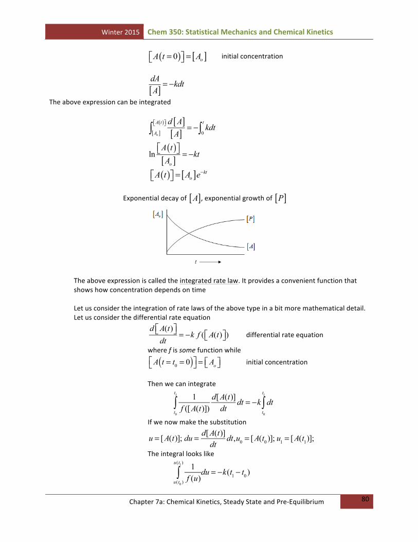
( ) [ ] ktoA t A e−=⎡ ⎤⎣ ⎦
Exponential decay of [ ]A , exponential growth of [ ]P
The above expression is called the integrated rate law. It provides a convenient function that shows how concentration depends on time Let us consider the integration of rate laws of the above type in a bit more mathematical detail. Let us consider the differential rate equation
d A(t)⎡⎣ ⎤⎦dt
= −k f ( A(t)⎡⎣ ⎤⎦) differential rate equation
where f is some function while
A t = t0 = 0( )⎡⎣ ⎤⎦ = Ao⎡⎣ ⎤⎦ initial concentration
Then we can integrate
1f ([A(t)])t0
t1
∫d[A(t)]
dtdt = −k dt
t0
t1
∫
If we now make the substitution
u = [A(t)]; du = d[A(t)]
dtdt,u0 = [A(t0 )]; u1 = [A(t1)];
The integral looks like
1f (u)u(t0 )
u(t1)
∫ du = −k(t1 − t0 )

Winter 2015 Chem 350: Statistical Mechanics and Chemical Kinetics
Chapter 7a: Chemical Kinetics, Steady State and Pre-‐Equilibrium
81
or substituting back u by A, and setting t0 = 0, t1 = t
1f ([A])[ A(t=0)]
[ A(t )]
∫ d[A]= −k(t − 0) = −kt
This is the general equation we can use when discussing single reactions. Example 18.4 in Reid and Engel
An interesting example of exponential decay is the determination of the age of fossils by monitoring decay of 14C . This is a very slow process ( 12 13.81 10k s− −= ⋅ )
Living cells exchange 14C with the environment, which has a constant 14C⎡ ⎤⎣ ⎦ from cosmic rays
(outer space).
The environment rate is −
d 14C⎡⎣ ⎤⎦dt
= k 14C⎡⎣ ⎤⎦ = 15.3 events / minute
Then
14 14
14 14
2.415.3
fossil fossil
o o
d C dt k C
d C dt k C
⎡ ⎤ ⎡ ⎤− ⎣ ⎦ ⎣ ⎦= =⎡ ⎤ ⎡ ⎤− ⎣ ⎦ ⎣ ⎦
(2.4 is supposedly measured)
14 14 kt
fossil oC C e−⎡ ⎤ ⎡ ⎤=⎣ ⎦ ⎣ ⎦
→using 12 13.81 10k s− −= ⋅ we obtain 114.86 10t s= ⋅ = 15 400 years
This is how carbon dating works. The idea is that 14C⎡ ⎤⎣ ⎦ is constant on the surface of the Earth over long periods of time (short on astronomical timescales) is crucial to the argument. The Earth takes up 14C⎡ ⎤⎣ ⎦ from outer space.
I will discuss more examples of increasing complexity. Setting up the differential rate equation is easy. Getting the integrated rate expression is tedious, and can only be done (without being a mathematician) for simple cases.
b) Second order – simplest 2k
A P→
− 1
2d A⎡⎣ ⎤⎦
dt= k A⎡⎣ ⎤⎦
2 →
[ ][ ]2
2d A
kdtA
−=
[ ][ ][ ]
( )2 2
o
A t
A
d Akt
A
⎡ ⎤⎣ ⎦− =∫
( ) [ ]1 1 2
o
ktAA t
− =⎡ ⎤⎣ ⎦
or ( ) [ ]1 1 2
o
ktAA t
= +⎡ ⎤⎣ ⎦
Plot ( )1A t⎡ ⎤⎣ ⎦
vs t yields a straight line, slope = 2k

Winter 2015 Chem 350: Statistical Mechanics and Chemical Kinetics
Chapter 7a: Chemical Kinetics, Steady State and Pre-‐Equilibrium
82
c) Second order – more complicated k
A B P+ →
[ ] [ ]oA A x= − P x=
[ ] [ ]oB B x= −
[ ] [ ][ ] [ ]( ) [ ]( )o o
d A dx k A B k A x B xdt dt
− = = = − −
[ ]( ) [ ]( )( )
0
x t
xo o
dx ktA x B x=
=− −∫
Difficult integral, how do you do it?
CAo⎡⎣ ⎤⎦ − x( ) +
DBo⎡⎣ ⎤⎦ − x( ) =
1Ao⎡⎣ ⎤⎦ − x( ) Bo⎡⎣ ⎤⎦ − x( )
Solve for the unknown constants C and D, multiply both sides by
Ao⎡⎣ ⎤⎦ − x( ) Bo⎡⎣ ⎤⎦ − x( ), →
[ ]( ) [ ]( ) 1o oC B x D A x− + − =
( ) 0x C D− + = D C= −
[ ] [ ]( ) 1o oC B A− = → [ ] [ ]( )
1
o o
CB A
=−
[ ] [ ]( ) [ ] [ ]
( )
0
1 1 1x t
xo oo o
dx ktA x B xB A =
⎛ ⎞− =⎜ ⎟⎜ ⎟− −− ⎝ ⎠
∫
[ ] [ ]( ) [ ]( ) [ ]( ) ( )
0
1 ln lnx t
o o xo o
B x A x ktB A =
⎡ ⎤− − − =⎣ ⎦−
[ ] [ ]( )
[ ][ ]
[ ][ ]
1 ln ln o
oo o
B Bkt
A AB A
⎡ ⎤⎛ ⎞ ⎛ ⎞− =⎢ ⎥⎜ ⎟ ⎜ ⎟⎜ ⎟ ⎜ ⎟− ⎢ ⎥⎝ ⎠ ⎝ ⎠⎣ ⎦
ln
B⎡⎣ ⎤⎦A⎡⎣ ⎤⎦
⎛
⎝⎜
⎞
⎠⎟ = ln
Bo⎡⎣ ⎤⎦Ao⎡⎣ ⎤⎦
⎛
⎝⎜
⎞
⎠⎟ + Bo − Ao( )kt
If o oB A= , the analysis is not correct. For that case ( ) [ ]1 1
o
ktAA t
= +⎡ ⎤⎣ ⎦
Differential equations quickly get complicated. Numerical solutions can always be obtained (Matlab!)
Half-‐life:

Winter 2015 Chem 350: Statistical Mechanics and Chemical Kinetics
Chapter 7a: Chemical Kinetics, Steady State and Pre-‐Equilibrium
83
Instead of rate constants one may speak of half-‐life. In my opinion this is most useful in the context of first-‐order exponential decay. By definition, the half-‐life is the time needed for half of the reactant to disappear. For first order reactions it gives a simple relation between halftime and rate constant:
[ ][ ]
2ln o
o
Ak
Aτ− =
ln 2k
τ = in seconds
Reversible reactions
Up to now, we only considered reactions that only go one way towards the products. In reality all reactions are reversible in principle. This is how one obtains chemical equilibrium. Let me discuss the simplest example. It will be clear quickly that we have to resort to numerical methods.
First order reversible reaction A
b
f
B
In these notes I use f for forward rates constants and b for backward rate constants. The differential rate laws are given by
[ ] [ ] [ ]d A
b B f Adt
= −
[ ] [ ] [ ]d B
f A b Bdt
= −
[ ] [ ] 0d A d Bdt dt
+ =
[ ] [ ]( ) 0d A Bdt
+ = A⎡⎣ ⎤⎦ + B⎡⎣ ⎤⎦ = 2Co 2Co :(some initial
concentration. The factor of 2 is for convenience below.)
At equilibrium [ ] 0d Adt
= → eq eqb B f A⎡ ⎤ ⎡ ⎤=⎣ ⎦ ⎣ ⎦
eq
eqeq
B fKbA
⎡ ⎤⎣ ⎦ = =⎡ ⎤⎣ ⎦
eqf K b=
This shows that the forward and backward rate constant are related by the thermodynamic equilibrium constant. Kinetics should be such that in limit of large t , equilibrium is reached. Solving the differential equation [ ] oB C x= +
[ ] oA C x= −

Winter 2015 Chem 350: Statistical Mechanics and Chemical Kinetics
Chapter 7a: Chemical Kinetics, Steady State and Pre-‐Equilibrium
84
[ ] [ ] [ ]d B dx f A b Bdt dt
= = −
[ ] [ ]o of C x b C x= − − +
( ) ( )of b C f b x= − − +
( ) ( )o
dx dtf b C f b x
=− − +
( )( )
( )o
dx f b dtf b
x Cf b
= − +−
−+
( )( )
( )
( )
( )0
lnx t
o
x
f bx C f b t
f b⎛ ⎞−
− = − +⎜ ⎟⎜ ⎟+⎝ ⎠
( ) ( )f b to o o
f b f bx t C x C ef b f b
− +⎛ ⎞⎛ ⎞ ⎛ ⎞− −= + −⎜ ⎟⎜ ⎟ ⎜ ⎟+ +⎝ ⎠ ⎝ ⎠⎝ ⎠
As t→∞ , ( ) of bx t Cf b
⎛ ⎞−= ⎜ ⎟+⎝ ⎠
Hence as t→∞
[ ][ ]
1221
oo
eqo
o
f bCB f bC x f f KA C x b bf bC
f b
∞
∞
⎛ ⎞−+⎜ ⎟++ ⎝ ⎠= = = = =− ⎛ ⎞−−⎜ ⎟+⎝ ⎠
It is seen that ( )x t shows exponential decay to equilibrium value, but details are cumbersome.
Interestingly the rate of reaching of equilibrium depends on (f+b). The decay happens as the sum of the forward and backward rates. To check and explore formulas, Matlab might be most appropriate. General discussion of kinetics Elementary reactions
An elementary reaction is a unimolecular or bimolecular reaction (higher order is not important. They do not contribute to the rate). Most importantly they have a differential rate law that follows stoichiometry. Unimolecular: Bimolecular: A B 2A C
A 2B 2A C + D A B +C A+ B C

Winter 2015 Chem 350: Statistical Mechanics and Chemical Kinetics
Chapter 7a: Chemical Kinetics, Steady State and Pre-‐Equilibrium
85
A+ B C + D All of these reactions can be expressed as
aA+ bB cC + dD , , ,a b c d : all integers (0 also possible)
R = dξ
dt= +k f A⎡⎣ ⎤⎦
aB⎡⎣ ⎤⎦
b− kb C⎡⎣ ⎤⎦
cD⎡⎣ ⎤⎦
d
fk and bk are the rate constants for the forward and backward reactions. I will use R
to denote the rate of the reaction.
From thermodynamics we can get a relation between fk and bk . At equilibrium the rate is 0,
or the forward and backward rates are equal.
c d a b
b eq eq f eq eqk C D k A B⎡ ⎤ ⎡ ⎤ ⎡ ⎤ ⎡ ⎤=⎣ ⎦ ⎣ ⎦ ⎣ ⎦ ⎣ ⎦
Or
c d
eq eq feqa b
beq eq
C D kK
kA B
⎡ ⎤ ⎡ ⎤⎣ ⎦ ⎣ ⎦ = =⎡ ⎤ ⎡ ⎤⎣ ⎦ ⎣ ⎦
f b eqk k K= , as seen before
From thermo, at a given ,P T
( )ln ,eq RRT K G P T= −Δ
We can get eqK from RGΔ . There is lots of experimental data to calculate this.
If one knows fk , bk and initial concentrations, one can simply integrate
d A⎡⎣ ⎤⎦dt
= −aR = −a k f A⎡⎣ ⎤⎦a
B⎡⎣ ⎤⎦b− kb C⎡⎣ ⎤⎦
cD⎡⎣ ⎤⎦
d⎡⎣⎢
⎤⎦⎥
d B⎡⎣ ⎤⎦dt
= −bR = −b k f A⎡⎣ ⎤⎦a
B⎡⎣ ⎤⎦b− kb C⎡⎣ ⎤⎦
cD⎡⎣ ⎤⎦
d⎡⎣⎢
⎤⎦⎥
d C⎡⎣ ⎤⎦dt
= +cR = +c k f A⎡⎣ ⎤⎦a
B⎡⎣ ⎤⎦b− kb C⎡⎣ ⎤⎦
cD⎡⎣ ⎤⎦
d⎡⎣⎢
⎤⎦⎥
d D⎡⎣ ⎤⎦dt
= +dR = +d k f A⎡⎣ ⎤⎦a
B⎡⎣ ⎤⎦b− kb C⎡⎣ ⎤⎦
cD⎡⎣ ⎤⎦
d⎡⎣⎢
⎤⎦⎥
[ ] [ ] [ ] [ ], , ,o o o oA B C D
This kind of first order differential equations are easy to solve on a computer
Let us now consider that we have a number of competing elementary reactions. This is what defines a reaction mechanism. The key is to derive a set of coupled differential equations. The rest can be done by computer. Let me proceed through an example. It concerns a mixture of 2H and 2Br reacting to HBr

Winter 2015 Chem 350: Statistical Mechanics and Chemical Kinetics
Chapter 7a: Chemical Kinetics, Steady State and Pre-‐Equilibrium
86
Set of elementary reactions (reaction mechanism):
1) Br2 2Br R1 = f1 Br2⎡⎣ ⎤⎦ − b1 Br⎡⎣ ⎤⎦2
2) H2 2H R2 = f2 H2⎡⎣ ⎤⎦ − b2 H⎡⎣ ⎤⎦2
3) Br + H2 HBr + H R3 = f3 Br⎡⎣ ⎤⎦ H2⎡⎣ ⎤⎦ − b3 H⎡⎣ ⎤⎦ HBr⎡⎣ ⎤⎦
4) H + Br2 HBr + Br R4 = f4 H⎡⎣ ⎤⎦ Br2⎡⎣ ⎤⎦ − b4 Br⎡⎣ ⎤⎦ HBr⎡⎣ ⎤⎦
5) H + Br HBr R5 = f5 H⎡⎣ ⎤⎦ Br⎡⎣ ⎤⎦ − b5 HBr⎡⎣ ⎤⎦
Using the expression for the rate of each reaction, we can write:
d Br2⎡⎣ ⎤⎦dt
= −R1 − R4
d Br⎡⎣ ⎤⎦dt
= 2R1 − R3 + R4 − R5
d H2⎡⎣ ⎤⎦dt
= −R2 − R3
d H⎡⎣ ⎤⎦dt
= 2R2 + R3 − R4 − R5
d HBr⎡⎣ ⎤⎦dt
= R3 + R4 + R5
Setting up the rate equations given a reaction mechanism (or set of elementary reactions) is a favorite exam question. You can check for possible errors by checking the so-‐called mass-‐balance. Atoms are conserved in chemical reactions, and so we can enumerate the total Br concentration and H concentration (or any other atom species in a reaction). For the above, we get:
[Br]total = [Br]+ 2[Br2]+ [HBr]= [Br(t = 0)]total = constant
d[Br]total
dt= 0 = d[Br]
dt+ 2
d[Br2]dt
+ d[HBr]dt
= (2R1 − R3 + R4 − R5)+ 2(−R1 − R4 )+ (R3 + R4 + R5)
= 0 indeed!
Likewise:
[H ]total = [H ]+ 2[H2]+ [HBr]= [H (t = 0)]total = constant
d[H ]total
dt= 0 = d[H ]
dt+ 2
d[H2]dt
+ d[HBr]dt
= (2R2 + R3 − R4 − R5)+ 2(−R2 − R3)+ (R3 + R4 + R5)
= 0
This is a good check (I would ask for this check on the exam). It is also a useful check when coding a reaction mechanism in matlab. If we supply initial concentrations for each of the 5 species in the reaction mixture:
[ ] [ ] [ ] [ ] [ ]2 2, , , ,Br H Br H HBr and we supply the values for the forward and backward rate
Winter 2015 Chem 350: Statistical Mechanics and Chemical Kinetics
Chapter 7a: Chemical Kinetics, Steady State and Pre-‐Equilibrium
87
constants ,i if b , it is a straightforward matter to solve the differential equations. (Matlab). We
can also note that for each elementary reaction we have a thermodynamic relation fi = Keq,ibi .
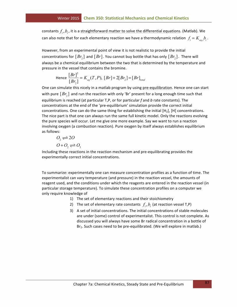
However, from an experimental point of view it is not realistic to provide the initial concentrations for [Br2] and [Br] . You cannot buy bottle that has only [Br2] . There will always be a chemical equilibrium between the two that is determined by the temperature and pressure in the vessel that contains the bromine.
Hence
[Br]2
[Br2]= Keq (T , P), [Br]+ 2[Br2]= [Br]total
One can simulate this nicely in a matlab program by using pre-‐equilibration. Hence one can start with pure [Br2] and run the reaction with only ‘Br’ present for a long enough time such that equilibrium is reached (at particular T,P, or for particular f and b rate constants). The concentrations at the end of the ‘pre-‐equilibrium’ simulation provide the correct initial concentrations. One can do the same thing for establishing the initial [H2], [H] concentrations. The nice part is that one can always run the same full kinetic model. Only the reactions evolving the pure species will occur. Let me give one more example. Say we want to run a reaction involving oxygen (a combustion reaction). Pure oxygen by itself always establishes equilibrium as follows:
O2 ! 2OO +O2 !O3
Including these reactions in the reaction mechanism and pre-‐equilibrating provides the experimentally correct initial concentrations. To summarize: experimentally one can measure concentration profiles as a function of time. The experimentalist can vary temperature (and pressure) in the reaction vessel, the amounts of reagent used, and the conditions under which the reagents are entered in the reaction vessel (in particular storage temperature). To simulate these concentration profiles on a computer we only require knowledge of
1) The set of elementary reactions and their stoichiometry 2) The set of elementary rate constants ,i if b (at reaction vessel T,P) 3) A set of initial concentrations. The initial concentrations of stable molecules
are under (some) control of experimentalist. This control is not complete. As discussed you will always have some Br radical concentration in a bottle of Br2. Such cases need to be pre-‐equilibrated. (We will explore in matlab.)
Winter 2015 Chem 350: Statistical Mechanics and Chemical Kinetics
Chapter 7a: Chemical Kinetics, Steady State and Pre-‐Equilibrium
88
Temperature dependence We can know the temperature and pressure dependence of
Keq,i typically. This knowledge stems either
from measurement, or from the use of thermochemistry data tables, or from calculating the data using quantum chemistry. We in general have access to RGΔ ln eq RRT K G→ = −Δ .
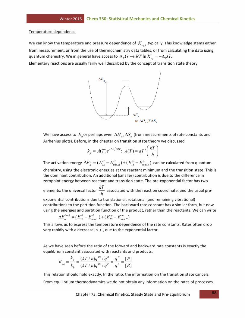
Elementary reactions are usually fairly well described by the concept of transition state theory
We have access to aE or perhaps even ,a aH SΔ Δ (from measurements of rate constants and Arrhenius plots). Before, in the chapter on transition state theory we discussed
k f = A(T )e−ΔEa
f / RT ; A(T ) = aT x kTh
⎛⎝⎜
⎞⎠⎟
The activation energy ΔEa
f = (ETSel − Emin,R
el )+ (ETSzp − Emin,R
zp ) can be calculated from quantum
chemistry, using the electronic energies at the reactant minimum and the transition state. This is the dominant contribution. An additional (smaller) contribution is due to the difference in zeropoint energy between reactant and transition state. The pre-‐exponential factor has two
elements: the universal factor kTh
associated with the reaction coordinate, and the usual pre-‐
exponential contributions due to translational, rotational (and remaining vibrational) contributions to the partition function. The back ward rate constant has a similar form, but now using the energies and partition function of the product, rather than the reactants. We can write
ΔEa
back = (ETSel − Emin,P
el )+ (ETSzp − Emin,P
zp ) This allows us to express the temperature dependence of the rate constants. Rates often drop very rapidly with a decrease in T , due to the exponential factor. As we have seen before the ratio of the forward and backward rate constants is exactly the equilibrium constant associated with reactants and products.
Keq =
k f
kb
= (kT / h) !qTS / qR
(kT / h) !qTS / qP = qP
qR = [P][R]
This relation should hold exactly. In the ratio, the information on the transition state cancels.
From equilibrium thermodynamics we do not obtain any information on the rates of processes.

Winter 2015 Chem 350: Statistical Mechanics and Chemical Kinetics
Chapter 7a: Chemical Kinetics, Steady State and Pre-‐Equilibrium
89
Detailed balance. There is one more subtlety I would like to discuss. As a reaction mixture reaches equilibrium the rates of each elementary reaction should reach zero. This is called detailed balance. If one chooses an arbitrary set of rate constants this doesn’t necessarily happen. One has to make sure the rate constants are consistent with thermodynamics! This is best illustrated by an example. Consider the following trio of elementary reactions:
A! B;[Beq ][Aeq ]
; K1 =f1
b1
A! C;[Ceq ][Aeq ]
; K2 =f2
b2
B! C;[Ceq ][Beq ]
; K3 =f3
b3
From a chemical perspective it is logical that if A is in equilibrium with both B and C, that also B and C must be in equilibrium. This provides a relation between the equilibrium constants. They are not all independent. It is easily seen that
K3 =
[Ceq ][Beq ]
=[Ceq ] / [Aeq ][Beq ] / [Aeq ]
=K2
K1
But this has the consequence that also the rate constants are not independent!
f3
b3
=K2
K1
=f2b1
b2 f1
If we define the rate constants using ratios of partition functions, it is easily seen that the rate constants necessarily satisfy the thermodynamic relationships, and therefore detailed balance would be satisfied. Let me give an example to illustrate the point. In the above example I will use EA, EB , EC to denote the ground state energies of each species (electronic + zeropoint),
and ETS to denote the energy of the transition state for the third reaction, while neglecting the difficult part of the pre-‐exponential rates. (Everything would be exactly correct if we use the complete ratios of partition functions).
f3
b3
≈(kT / h)exp(−(ETS − EB ) / RT )(kT / h)exp(−(ETS − EC ) / RT )
= exp(−(EC − EB ) / RT ) = K3
=K2
K1
=exp(−(EC − EA) / RT )exp(−(EB − EA) / RT )
= exp(−(EC − EB ) / RT )
If we always define rates using energies of each species, and energies of transition states, everything works out and detailed balance is satisfied. We will explore what happens if the rate constants are inconsistent in an exercise. The reaction still reaches chemical equilibrium, but the individual rates do not vanish! Weird. Let me summarize.

Winter 2015 Chem 350: Statistical Mechanics and Chemical Kinetics
Chapter 7a: Chemical Kinetics, Steady State and Pre-‐Equilibrium
90
Connections to experiment: Vary initial concentrations of reagents, T , measure concentration profiles or measure initial rates.
-‐ Postulate a set of elementary chemical reactions -‐ Set up a set of differential equations to solve for concentration profiles (use
computer). -‐ Use thermodynamic data to get relations between ,f bk k
-‐ Fit the (independent) rate constants at a given fixed temperature to measured reaction profile
-‐ Vary temperature to obtain the temperature dependence of ,f bk k
-‐ Extract activation energies (and possibly ,a aH SΔ Δ )
In Matlab we could test the procedure: I might provide a subroutine that will generate concentration profiles depending on T , initial concentrations. You (the user) could set some initial concentrations to zero, or use excess reagent etc, and run the kinetics simulation. But you cannot look at the subroutine to see what it does. I might add some noise to the data (as in real experiments). By exploring the generated data, you may:
1) Figure out the set of elementary reactions 2) Fit the rate constants 3) Determine temperature dependence of rate constants
Using a computer intelligently would assist enormously in the task. This is too much to learn in this class, but we will explore some of the steps involved using Matlab. The principles can be laid out, but there is no time to really teach you the ‘skills’ needed (I would have to learn myself). Note added: We are currently working on such a simulation tool. It is called C.K. Watson (Chemical Kinetics Watson). I hope to use it in class to give you some idea of the logical thinking processes involved. You can think of unraveling the chemical kinetics model as a detective story (hence the involvement of Watson). The computer (C.K. Watson) does all the tedious part of the work (including running the kinetics experiment). You, Sherlock, put all the pieces together and solve the puzzle: What are the set of reactions involved? “Elementary my dear Watson!”
Steady State and Pre-‐equilibrium Approximation
If a full set of elementary reactions is known (and their rate constants) it is quite straightforward to set up the rate equations to solve (numerically) for the reaction profiles. The solutions would also depend on initial concentrations. This I think is the most important message to take away. In much of the remainder of our discussion of kinetics, we wish to understand certain features more intuitively. For this reason, approximate solutions are sought that can provide additional insight (and analytical formulas).

Winter 2015 Chem 350: Statistical Mechanics and Chemical Kinetics
Chapter 7a: Chemical Kinetics, Steady State and Pre-‐Equilibrium
91
This part of kinetics is a bit ‘art-‐ful’. One might derive different solutions depending on the path one takes. They are all only approximations. Here we discuss the steady state and pre-‐equilibrium approximations. Let’s consider the following reactions:
A
b1
f1I [ ] [ ]1 1 1r f A b I= −
I→
f2
P ( 2b very small) [ ]2 2r f I=
A is first converted to some intermediate, which then reacts to products. The kinetics is described by the following set of differential equations
[ ] [ ] [ ]1 1 1
d Ar f A b I
dt= − = − +
[ ] [ ] [ ] [ ]1 2 1 1 2
d Ir r f A b I f I
dt= − = − −
[ ] [ ]2 2
d Pr f I
dt= =
For any values of 1 1 2, ,f b f one can solve the equations numerically
Under 2 limiting scenarios, one can get expressions for the rate [ ]d Pdt
, which is how one uses
this. a) Steady State Approximation ( f2 fast)
In this approximation one assumes [ ] 0d Idt
= . The physical assumption is that [ ]I is fairly
small, and after an initial rise (at time 0) it reaches a constant plateau. It is consumed as fast as it is produced. In general this approximation is applied to every intermediate in the set of reactions. It allows one to eliminate intermediates, by expressing their concentrations in terms of others. For the present example: 2 1r r= 1r : production of I , 2r : consumption of I
[ ] 0d Idt
= → 1 2 0r r− =
[ ] [ ] [ ] ( )[ ]1 1 2 1 2f A b I f I b f I= + = +
[ ] [ ]1
1 2
fI Ab f
=+
Then [ ] [ ] [ ]1 1
d Ab I f A
dt= −

Winter 2015 Chem 350: Statistical Mechanics and Chemical Kinetics
Chapter 7a: Chemical Kinetics, Steady State and Pre-‐Equilibrium
92
= − f1 1−
b1
f2 + b1
⎛⎝⎜
⎞⎠⎟
A⎡⎣ ⎤⎦ = − f1(f2 + b1 − b1
f2 + b1
) A⎡⎣ ⎤⎦
[ ]effk A= − 1 2
2 1eff
f fkf b
=+
To Solve: [ ] [ ] effk t
oA A e−=
[ ] [ ] [ ] [ ]oP A A I= − −
[ ] [ ] [ ]1 1
2 1 2 1
effk to
f fI A A ef b f b
−= =+ +
[ ] [ ] 1
2 1
1 eff effk t k to
fP A e ef b
− −⎛ ⎞= − −⎜ ⎟+⎝ ⎠
Note: we derived kinetics setting [ ] 0d Idt
= → [ ] [ ]1
2 1
fI Af b
=+
, but [ ] ( )A A t= ⎡ ⎤⎣ ⎦ , hence
after solution [ ] 0d Idt
≠ . This is a little strange. I prefer my math to be consistent!
We can also analyze situation in the limit 1 0b →
2 11
2 1eff
f fk ff b
= →+
[ ] [ ]1
2
fI Af
=
[ ] [ ] 1
2
1 1effk to
fP A ef
−⎛ ⎞⎛ ⎞= − +⎜ ⎟⎜ ⎟⎜ ⎟⎝ ⎠⎝ ⎠
b) Pre-‐equilibrium ( 2f slow)
A
b1
f1I [ ] [ ]1 1 1r f A b I= −
2f
I P→ ( 2b very small) [ ]2 2r f I=
If 2f is very small (slow), then the equilibrium between A I can be maintained and this slowly leaks away to products
[ ] [ ] [ ]1 1 1
d Ar f A b I
dt= − = − +
[ ] [ ] [ ] [ ]1 2 1 1 2
d Ir r f A b I f I
dt= − = − −
[ ] [ ]2 2
d Pr f I
dt= =

Winter 2015 Chem 350: Statistical Mechanics and Chemical Kinetics
Chapter 7a: Chemical Kinetics, Steady State and Pre-‐Equilibrium
93
The assumption of [ ]A and [ ]I
in equilibrium translates to
[ ] [ ]1 1f A b I= → [ ] [ ]1
1
fI A
b=
→ [ ] 0d Adt
= ?? (again, strange! A is supposed to react!)
[ ] [ ]20d I
f Idt
= −
[ ] [ ] [ ]2 1
21
d P f ff I Adt b
= =
[ ] ( ) [ ] [ ]1
1o o
fP A A I A A Ab
⎛ ⎞= − − = − −⎜ ⎟
⎝ ⎠
[ ] [ ] [ ]1 2 1
1 1
1d P d Af f f Adt b dt b
⎛ ⎞= − + =⎜ ⎟
⎝ ⎠
[ ] [ ]2 1 1
1 1 1
d A f f b Adt b b f
= − ⋅+
( ) [ ]2 1
1 1
f f Ab f
= −+
( )
( )2 1
1 1
beff
f fkb f
=+
(pre-‐equilibrium (b), different from steady state before (a)
[ ] [ ]( )beffk t
oA A e−=
[ ] [ ]( )
1
1
beffk t
ofI A eb
−⎛ ⎞= ⎜ ⎟⎝ ⎠
[ ] [ ] [ ] [ ]( )
1
1
1 1beffk t
o ofP A A I A eb
−⎛ ⎞⎛ ⎞= − − = − +⎜ ⎟⎜ ⎟⎜ ⎟⎝ ⎠⎝ ⎠
You can see that steady state and pre-‐equilibrium approximations lead to different behavior. Neither is quite right. Moreover, both approximations are not all consistent.
Here: [ ] 0d Adt
= from rate law and pre equilibrium condition.
We do not use this equation, but analyze in terms of [ ]d Pdt
.

Winter 2015 Chem 350: Statistical Mechanics and Chemical Kinetics
Chapter 7a: Chemical Kinetics, Steady State and Pre-‐Equilibrium
94
I am not entirely comfortable with the math we do. Here, I would not be surprised if for complicated cases one might get a different result depending on how one goes about doing it. As I said, kinetics can be a bit art-‐ful. The issue is that chemical kinetics is an ancient topic, well-‐developed before the advent of computers. In those days scientists had to make approximations in order to solve their problems. This is no longer true today. My take on it: use computers to do the hard work. Let us consider the rational for approximations
A
b1
f1I→
f2
P
a) 2f is slow, hence [ ]A and [ ]I are in equilibrium, after some initialization time → pre-‐
equilibrium
b) [ ] 0d Idt
= steady state. [ ]I after some initialization is produced and consumed at equal
rates: [ ] ( )[ ]1 2 1f A f b I= +
In both approximations we can eliminate[ ]I , and then solve for ( )A t⎡ ⎤⎣ ⎦ . Both approximations
are used extensively to obtain analytical integrated rates. These are traditionally favourite questions on exams. You can tell I am not all that impressed by this cleverness. We will test some of the approximations used in Matlab. On the exam I am most likely to ask you to set up the differential rate equations (how you would program it in matlab).