Embed Size (px)
Citation preview
Chapter 7

Chapter Summary � Introduction to Discrete Probability � Probability Theory � Bayes’ Theorem

Section 7.1

Sec.on Summary � Finite Probability � Probabilities of Complements and Unions of Events

Probability of an Event We first study Laplace’s classical theory of probability, which he introduced in the 18th century, when he analyzed games of chance.
� We define these key terms: � An experiment is a procedure that yields one of a given set of
possible outcomes. � The sample space of the experiment is the set of possible
outcomes. � An event is a subset of the sample space.
Definition: If S is a finite sample space of equally likely outcomes, and E is an event, that is, a subset of S, then the probability of E is p(E) = |E|/|S|.
� For every event E, we have 0 ≤ p(E) ≤ 1. This follows directly from the de=inition because 0 ≤ p(E) = |E|/|S| ≤ |S|/|S| ≤ 1, since 0 ≤ |E| ≤ |S|.
Pierre-‐Simon Laplace (1749-‐1827)

Applying Laplace’s Defini.on Example: An urn contains four blue balls and five red balls. What is the probability that a ball chosen from the urn is blue?
Example: What is the probability that when two dice are rolled, the sum of the numbers on the two dice is 7?

Applying Laplace’s Defini.on Example: An urn contains four blue balls and five red balls. What is the probability that a ball chosen from the urn is blue?
Solution: The probability that the ball is chosen is 4/9 since there are 9 possible outcomes, and 4 of these produce a blue ball.
Example: What is the probability that when two dice are rolled, the sum of the numbers on the two dice is 7?
Solution: By the product rule there are 62 = 36 possible outcomes. Six of these sum to 7. Hence, the probability of obtaining a 7 is 6/36 = 1/6.

Applying Laplace’s Defini.on Example: In a lottery, a player wins a large prize when they pick four digits that match, in correct order, four digits selected by a random mechanical process (repeats are allowed). What is the probability that a player wins the prize?
A smaller prize is won if exactly three digits are matched. What is the probability that a player wins the small prize?

Applying Laplace’s Defini.on Example: In a lottery, a player wins a large prize when they pick four digits
that match, in correct order, four digits selected by a random mechanical process (repeats are allowed). What is the probability that a player wins the prize?
Solution: By the product rule there are 10^4 = 10,000 ways to pick four digits. � Since there is only 1 way to pick the correct digits, the probability of winning
the large prize is 1/10,000 = 0.0001.
A smaller prize is won if exactly three digits are matched. What is the probability that a player wins the small prize?
Solution: If exactly three digits are matched, one of the four digits must be incorrect and the other three digits must be correct. For the digit that is incorrect, there are 9 possible choices (all except the correct digit).
The digit that is incorrect can be in any of 4 positions. Hence, by the sum rule, there a total of 36 possible ways to choose four digits that match exactly three of the winning four digits. The probability of winning the small price is 36/10,000 = 9/2500 = 0.0036.

Applying Laplace’s Defini.on Example: There are many lotteries that award prizes to people who correctly choose a set of six numbers out of the first n positive integers, where n is usually between 30 and 60. What is the probability that a person picks the correct six numbers out of 40?

Applying Laplace’s Defini.on Example: There are many lotteries that award prizes to people who correctly choose a set of six numbers out of the first n positive integers, where n is usually between 30 and 60. What is the probability that a person picks the correct six numbers out of 40?
Solution: The number of ways to choose six numbers out of 40 is
C(40,6) = 40!/(34!6!) = 3,838,380. There is only one winning combination. Hence, the probability of picking a winning combination is 1/ 3,838,380 ≈ 0.00000026.
Can you work out the probability of winning the lottery with the biggest prize where you live?

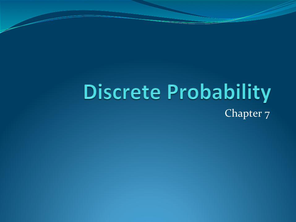
Applying Laplace’s Defini.on Example: What is the probability that the numbers 11, 4, 17, 39, and 23 are drawn in that order from a bin with 50 balls labeled with the numbers 1,2, …, 50 if a) The ball selected is not returned to the bin. b) The ball selected is returned to the bin before the next
ball is selected.
Applying Laplace’s Defini.on Example: What is the probability that the numbers 11, 4, 17, 39, and 23 are drawn in that order from a bin with 50 balls labeled with the numbers 1,2, …, 50 if a) The ball selected is not returned to the bin. b) The ball selected is returned to the bin before the next ball
is selected. Solution: Use the product rule in each case.
a) Sampling without replacement: The probability is 1/254,251,200 since there are 50 ∙49 ∙ 48 .47 ∙46 = P(50, 5) =254,251,200 ways to choose the five balls.
b) Sampling with replacement: The probability is 1/505 = 1/312,500,000 since 505 = 312,500,000.

The Probability of Complements and Unions of Events Theorem 1: Let E be an event in sample space S. The probability of the event = S − E, the complementary event of E, is given by
Proof: Using the fact that | | = |S| − |E|,

The Probability of Complements and Unions of Events Example: A sequence of 10 bits is chosen randomly. What is the probability that at least one of these bits is 0?

The Probability of Complements and Unions of Events Example: A sequence of 10 bits is chosen randomly. What is the probability that at least one of these bits is 0?
Solution: Let E be the event that at least one of the 10 bits is 0. Then is the event that all of the bits are 1s. The size of the sample space S is 210. Hence,

The Probability of Complements and Unions of Events Theorem 2: Let E1 and E2 be events in the sample space S. Then
Proof: Given the inclusion-‐exclusion formula from Section 2.2, |A ∪ B| = |A| + | B| − |A ∩ B|, it follows that

Example: What is the probability that a positive integer selected at random from the set of positive integers not exceeding 100 is divisible by either 2 or 5?
Solution: Let E1 be the event that the integer is divisible by 2 and E2 be the event that it is divisible 5? Then the event that the integer is divisible by 2 or 5 is E1 ∪ E2 and E1 ∩ E2 is the event that it is divisible by 2 and 5.
It follows that: p(E1 ∪ E2) = p(E1) + p(E2) – p(E1 ∩ E2) = 50/100 + 20/100 − 10/100 = 3/5.
The Probability of Complements and Unions of Events

Monty Hall Puzzle Example: You are asked to select one of the three doors to open. There is a large prize behind one of the doors and if you select that door, you win the prize. After you select a door, the game show host opens one of the other doors (which he knows is not the winning door). The prize is not behind the door and he gives you the opportunity to switch your selection. Should you switch?
1 32
Monty Hall Puzzle Example: You are asked to select one of the three doors to open.
There is a large prize behind one of the doors and if you select that door, you win the prize. After you select a door, the game show host opens one of the other doors (which he knows is not the winning door). The prize is not behind the door and he gives you the opportunity to switch your selection. Should you switch?
Solution: You should switch. The probability that your initial pick is
correct is 1/3. This is the same whether or not you switch doors. Since the game show host always opens a door that does not have the
prize, if you switch the probability of winning will be 2/3, because you win if your initial pick was not the correct door and the probability your initial pick was wrong is 2/3.
1 32
(This is a notoriously confusing problem that has been the subject of much discussion . Do a web search to see why!)

Section 7.2

Sec.on Summary � Assigning Probabilities � Probabilities of Complements and Unions of Events � Conditional Probability � Independence � Bernoulli Trials and the Binomial Distribution

Assigning Probabili.es Laplace’s definition from the previous section, assumed that all outcomes were equally likely. Now we introduce a more general definition of probabilities that avoids this restriction.
� Let S be a sample space of an experiment with a finite number of outcomes. We assign a probability p(s) to each outcome s, so that:
i. 0 ≤ p(s) ≤ 1 for each s ∈ S ii.
� The function p from the set of all outcomes of the sample space S is called a probability distribution.

Assigning Probabili.es Example: What probabilities should we assign to the outcomes H (heads) and T (tails) when a fair coin is flipped? What probabilities should be assigned to these outcomes when the coin is biased so that heads comes up twice as often as tails?
Solution: For the biased coin, we have p(H) = 2p(T). Because p(H) + p(T) = 1, it follows that 2p(T) + p(T) = 3p(T) = 1. Hence, p(T) = 1/3 and p(H) = 2/3.

Uniform Distribu.on Definition: Suppose that S is a set with n elements. The uniform distribution assigns the probability 1/n to each element of S. (Note that we could have used Laplace’s definition here.)
Example: Consider again the coin flipping example, but with a fair coin. Now p(H) = p(T) = 1/2.

Probability of an Event Definition: The probability of the event E is the sum of the probabilities of the outcomes in E.
� Note that now no assumption is being made about the distribution.
Example Example: Suppose that a die is biased so that 3 appears twice as often as each other number, but that the other five outcomes are equally likely. What is the probability that an odd number appears when we roll this die?
Solution: We want the probability of the event E = {1,3, 5}. We have p(3) = 2/7 and
p(1) = p(2) = p(4) = p(5) = p(6) = 1/7. Hence, p(E) = p(1) + p(3) + p(5) = 1/7 + 2/7 + 1/7 = 4/7.

Probabili.es of Complements and Unions of Events � Complements: still holds. Since each outcome is in either E or , but not both,
� Unions: also still holds under the new definition.

Combina.ons of Events Theorem: If E1, E2, … is a sequence of pairwise disjoint events in a sample space S, then
see Exercises 36 and 37 for the proof

Condi.onal Probability Definition: Let E and F be events with p(F) > 0. The conditional probability of E given F, denoted by P(E|F), is defined as:
Example: A bit string of length four is generated at random so that each of the 16 bit strings of length 4 is equally likely. What is the probability that it contains at least two consecutive 0s, given that its first bit is a 0?
Solution: Let E be the event that the bit string contains at least two consecutive 0s, and F be the event that the first bit is a 0. � Since E ⋂ F = {0000, 0001, 0010, 0011, 0100}, p(E⋂F)=5/16. � Because 8 bit strings of length 4 start with a 0, p(F) = 8/16= ½.
Hence,

Condi.onal Probability Example: What is the conditional probability that a family with two children has two boys, given that they have at least one boy. Assume that each of the possibilities BB, BG, GB, and GG is equally likely where B represents a boy and G represents a girl.

Condi.onal Probability Example: What is the conditional probability that a family with two children has two boys, given that they have at least one boy. Assume that each of the possibilities BB, BG, GB, and GG is equally likely where B represents a boy and G represents a girl.
Solution: Let E be the event that the family has two boys and let F be the event that the family has at least one boy. Then E = {BB}, F = {BB, BG, GB}, and E ⋂ F = {BB}. � It follows that p(F) = 3/4 and p(E⋂F)=1/4.
Hence,
Independence � Two events are independent if the occurrence of one of the events gives us no information about whether or not the other event will occur; that is, the events have no influence on each other.
� In probability theory we say that two events, E and F, are independent if the probability that they both occur is equal to the product of the probabilities of the two individual events

Independence Definition: The events E and F are independent if and only if
Note that if E and F are independent events then P(E/F) = P(E) and P(F/E) = P(F) The conditional probability of E happening, given that F has happened, is exactly the same as the probability of E.
E is not affected by F.
p(E⋂F) = p(E)p(F).

Independence Definition: The events E and F are independent if and only if Example: Suppose E is the event that a randomly generated bit string
of length four begins with a 1 and F is the event that this bit string contains an even number of 1s. Are E and F independent if the 16 bit strings of length four are equally likely?
Solution: There are eight bit strings of length four that begin with a 1, and eight bit strings of length four that contain an even number of 1s. � Since the number of bit strings of length 4 is 16, � Since E⋂F = {1111, 1100, 1010, 1001}, p(E⋂F) = 4/16=1/4.
We conclude that E and F are independent, because p(E⋂F) =1/4 = (½) (½)= p(E) p(F)
p(E⋂F) = p(E)p(F).
p(E) = p(F) = 8/16 = ½.

Gambler’s Fallacy � Gambler’s Falacy = The belief that if deviations from expected behaviour are observed in repeated independent trials of some random process, then future deviations in the opposite direction are more likely.
� Fair coin tossing: The probability of getting heads in a toss is ½ � The probability of getting 3 heads in a row is 1/8 � Suppose we tossed 4 heads in a row. What is the probability that the 5th toss is a head?
� A believer in Gambler’s Falacy may think the less toss is more likely to be a tail. However, this is not true.
� P(A5 | A1 & A2 & A3 & A4) = P(A5) = ½ � The events “five heads in a row” and “four heads then tails” are equally likely, with probability 1/32.

Why probability is ½ for a fair coin � While the probability of getting 5 heads in a row is only 1/32, it is only that before the coin is tossed the first time
� After the first four tosses, these four are no longer unknown events, and their probabilities become 1
� Thus, the probability of flipping a head after having already flipped 4 heads in a row is 1 x 1 x 1 x 1 x 1⁄∕2 = 1/2.
� Reasoning that it is more likely that the next toss will be a tail rather than head due to past tosses, that a run of luck in the past somehow influences the future, is the fallacy.
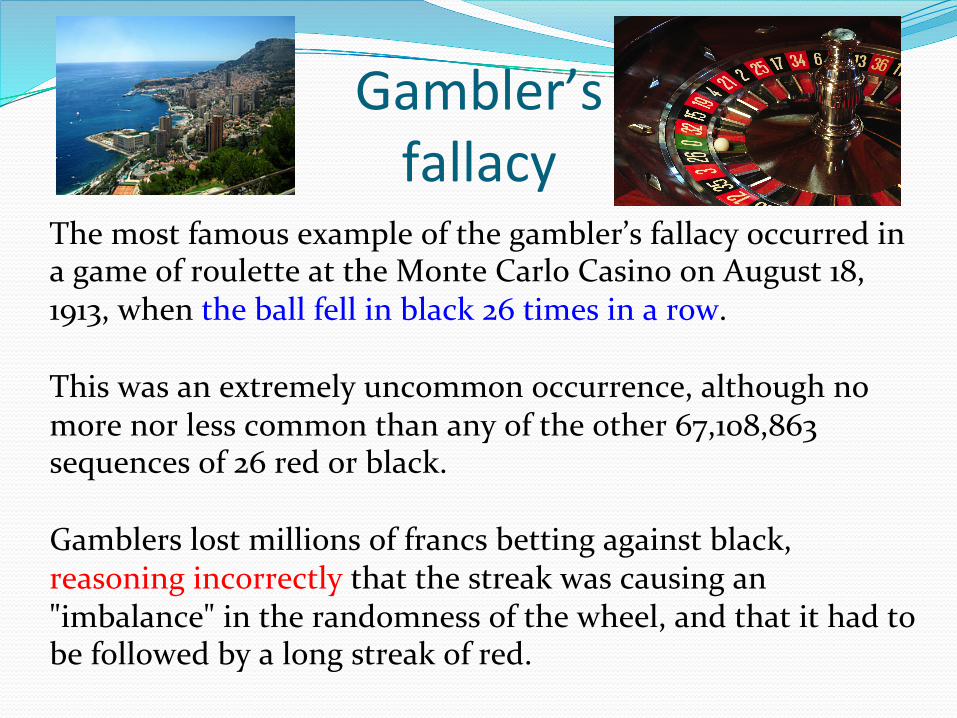
Gambler’s fallacy
The most famous example of the gambler’s fallacy occurred in a game of roulette at the Monte Carlo Casino on August 18, 1913, when the ball fell in black 26 times in a row. This was an extremely uncommon occurrence, although no more nor less common than any of the other 67,108,863 sequences of 26 red or black. Gamblers lost millions of francs betting against black, reasoning incorrectly that the streak was causing an "imbalance" in the randomness of the wheel, and that it had to be followed by a long streak of red.

Independence Example: Assume (as in the previous example) that each of the four ways a family can have two children (BB, GG, BG,GB) is equally likely. Are the events E, that a family with two children has two boys, and F, that a family with two children has at least one boy, independent?
Solution: Because E = {BB}, p(E) = 1/4. We saw previously that that p(F) = 3/4 and p(E⋂F)=1/4. The events E and F are not independent since
p(E) p(F) = 3/16 ≠ 1/4= p(E⋂F) .

Pairwise and Mutual Independence Definition: The events E1, E2, …, En are pairwise independent if and only if p(Ei⋂Ej) = p(Ei) p(Ej) for all pairs i and j with i ≤ j ≤ n.
The events are mutually independent if
whenever ij, j = 1,2,…., m, are integers with 1 ≤ i1 < i2 <∙∙∙ < im ≤ n and m ≥ 2.

Bernoulli Trials
James Bernoulli (1654 – 1705)
Definition: Suppose an experiment can have only two possible outcomes, e.g., the flipping of a coin or the random generation of a bit. � Each performance of the experiment is called a Bernoulli trial.
� One outcome is called a success and the other a failure. � If p is the probability of success and q the probability of failure, then p + q = 1.
� Many problems involve determining the probability of k successes when an experiment consists of n mutually independent Bernoulli trials.
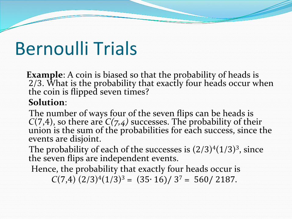
Bernoulli Trials Example: A coin is biased so that the probability of heads is 2/3. What is the probability that exactly four heads occur when the coin is flipped seven times?
Solution: The number of ways four of the seven flips can be heads is C(7,4), so there are C(7,4) successes. The probability of their union is the sum of the probabilities for each success, since the events are disjoint.
The probability of each of the successes is (2/3)4(1/3)3, since the seven flips are independent events.
Hence, the probability that exactly four heads occur is C(7,4) (2/3)4(1/3)3 = (35∙ 16)/ 37 = 560/ 2187.
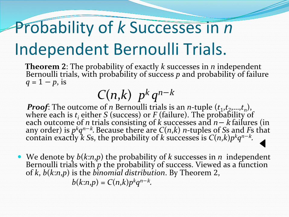
Probability of k Successes in n Independent Bernoulli Trials. Theorem 2: The probability of exactly k successes in n independent
Bernoulli trials, with probability of success p and probability of failure q = 1 − p, is
C(n,k) pk qn−k Proof: The outcome of n Bernoulli trials is an n-‐tuple (t1,t2,…,tn),
where each is ti either S (success) or F (failure). The probability of each outcome of n trials consisting of k successes and n− k failures (in any order) is pkqn−k. Because there are C(n,k) n-‐tuples of Ss and Fs that contain exactly k Ss, the probability of k successes is C(n,k)pkqn−k.
� We denote by b(k:n,p) the probability of k successes in n independent
Bernoulli trials with p the probability of success. Viewed as a function of k, b(k:n,p) is the binomial distribution. By Theorem 2,
b(k:n,p) = C(n,k)pkqn−k.

Binomial distribu.on for various p
Section 7.3

Sec.on Summary � Bayes’ Theorem � Generalized Bayes’ Theorem � Bayesian Spam Filters

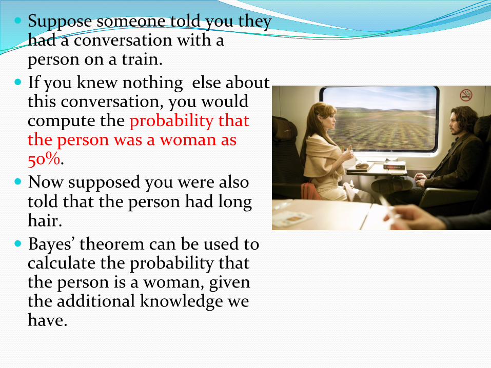
� Suppose someone told you they had a conversation with a person on a train.
� If you knew nothing else about this conversation, you would compute the probability that the person was a woman as 50%.
� Now supposed you were also told that the person had long hair. It is now more likely that the person was a woman, since women are more likely than men to have long hair.
� Bayes’ theorem can be used to calculate the probability that the person is a woman, given the additional knowledge we have.
Mo.va.on for Bayes’ Theorem “Bayes’ theorem is to the theory of probability what Pythagoras’ theorem is to geometry” (Sir Harold Jeffreys) � Bayes’ theorem allows us to use probability to answer questions such as the following: � Given that someone tests positive for having a particular disease, what is the probability that they actually do have the disease?
� Given that someone tests negative for the disease, what is the probability, that in fact they do have the disease?
� Bayes’ theorem has applications to medicine, law, artificial intelligence, engineering, and many diverse other areas.
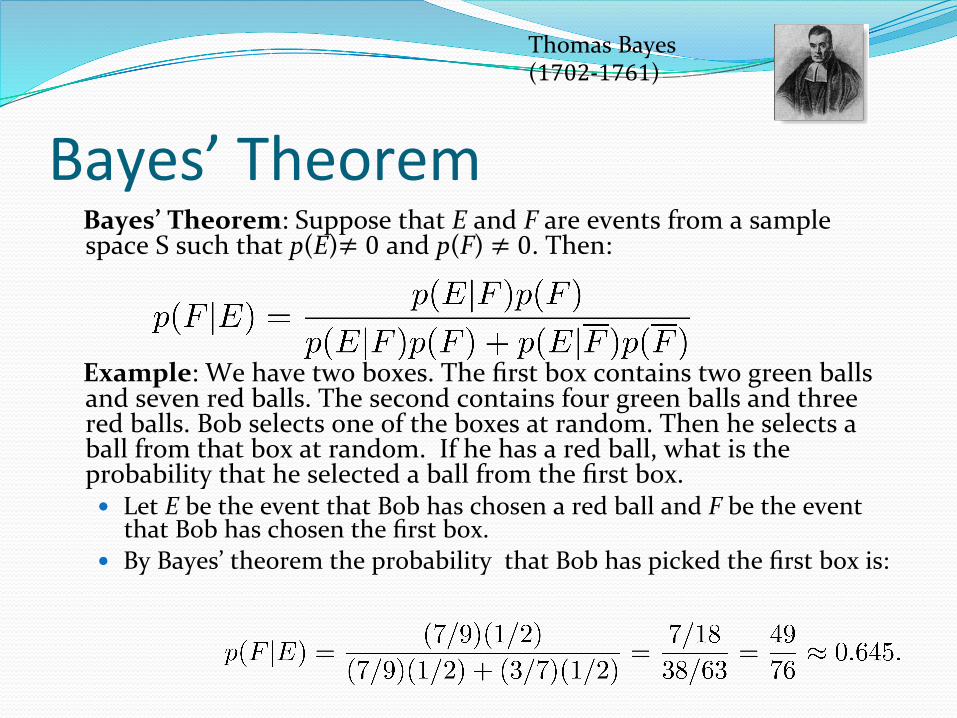
Bayes’ Theorem Bayes’ Theorem: Suppose that E and F are events from a sample
space S such that p(E)≠ 0 and p(F) ≠ 0. Then:
Example: We have two boxes. The first box contains two green balls and seven red balls. The second contains four green balls and three red balls. Bob selects one of the boxes at random. Then he selects a ball from that box at random. If he has a red ball, what is the probability that he selected a ball from the first box. � Let E be the event that Bob has chosen a red ball and F be the event
that Bob has chosen the first box. � By Bayes’ theorem the probability that Bob has picked the first box is:
Thomas Bayes (1702-‐1761)

Proof of Bayes’ Theorem � Recall the definition of the conditional probability p(E|F):
� From this definition, it follows that:
,
continued →

Proof of Bayes’ Theorem On the last slide we showed that
continued →
,
,
Solving for p(E|F) and for p(F|E) tells us that
Equating the two formulas for p(E F) shows that

Proof of Bayes’ Theorem On the last slide we
showed that:
Note that
Hence,
since
because and
By the definition of conditional probability,

Simple form of Bayes’ Theorem
A blue neon sign at the Autonomy Corporation, Cambridge, showing the simple statement of Bayes’ Theorem.

Interpreta.on of the Simple Form of Bayes’ Theorem � Bayes’ Theorem links the degree of belief in a proposition before and after accounting for evidence.
� Proposition A, Evidence B � P(A) = prior probability = initial degree of belief in A � P(A|B) = posterior probability = degree of belief in A after having accounted for B
� P(B|A)/P(B) = the support B provides for A � P(A|B) = P(B|A) x P(A) / (P(B) = [P(B|A)/P(B)] x P(A)
� Suppose someone told you they had a conversation with a person on a train.
� If you knew nothing else about this conversation, you would compute the probability that the person was a woman as 50%.
� Now supposed you were also told that the person had long hair.
� Bayes’ theorem can be used to calculate the probability that the person is a woman, given the additional knowledge we have.

How to solve the train problem � W = the conversation partner is a woman � L = the conversation partner has long hair � P(W|L) = [P(L|W) x P(W)]/ [P(L|W) x P(W) + P(L|Ŵ) x P(Ŵ)] Suppose we know 75% of women have long hair and 15% of men have long hair Then P(L|W) = 0.75 and P(L|Ŵ) = 0.15. P(W|L) = (o.75 x 0.5)/(0.75 x 0.5 + 0.15 x 0.5) = 0.83

Applying Bayes’ Theorem Example: Suppose that one person in 100,000 has a particular disease. There is a test for the disease that gives a positive result 99% of the time when given to someone with the disease. When given to someone without the disease, the test gives a negative result 99.5% of the time. Find: a) the probability that a person who test positive has the
disease. b) the probability that a person who test negative does
not have the disease. � Should someone who tests positive be worried?
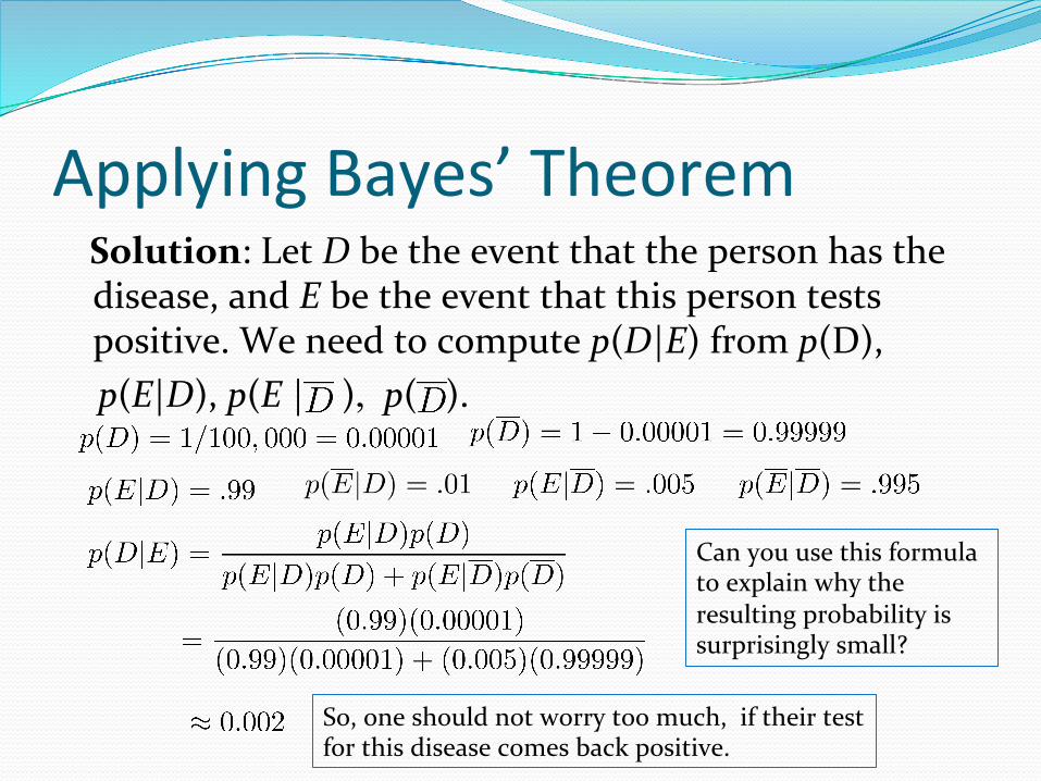
Applying Bayes’ Theorem Solution: Let D be the event that the person has the disease, and E be the event that this person tests positive. We need to compute p(D|E) from p(D),
p(E|D), p(E | ), p( ).
So, one should not worry too much, if their test for this disease comes back positive.
Can you use this formula to explain why the resulting probability is surprisingly small?

Interpreta.on of results � P(E|D) P(D) = P(test+| disease) P(disease) => true positive � P(E|Ď) P(Ď) = P(test+| no disease) P(no disease)=>false positive
P(D|E) = P(disease|test+) = (by Bayes’ Theorem)= = P(test+|disease) P(disease) /[P(test+|disease) P(disease) + P(test+| no disease) P(no disease)] = = P(true positives)/ (P(true positives) + P(false positives)) Because the disease is so rare, P(true positives) is small and P(false positives) is big, so: P(disease|test+) = small #/(small # + big #) = small

Applying Bayes’ Theorem � What if the result is negative?
� So, it is extremely unlikely one has the disease if one tests negative.
So, the probability one has the disease if they test negative is

Interpreta.on of results � P(Ē|Ď) P(Ď) = P(test-‐|no disease) P(no disease)=> true negative � P(Ē|D) P(D) = P(test-‐| disease) P(disease) => false negative � P(Ď|Ē) = P(no disease| test-‐) = (by Bayes’ theorem)= = P(test-‐|no disease) P(no disease)/ [P(test-‐)|no disease) P(no disease)+P(test-‐|disease) P(disease)] = P(true negatives) /P(true negatives) + P(false negatives)) Because the disease is so rare, # false negatives is small and number of # true negatives is big so: P(no disease|test-‐) = big #/ (big # + small #) = close to 1

Generalized Bayes’ Theorem Generalized Bayes’ Theorem: Suppose that E is an event from a sample space S and that F1, F2, …, Fn are mutually exclusive events such that
Assume that p(E) ≠ 0 for i = 1, 2, …, n. Then
Exercise 17 asks for the proof.

Bayesian Spam Filters � How do we develop a tool for determining whether an email is likely to be spam?
� If we have an initial set B(ad) of spam messages and set G(ood) of non-‐spam messages. We can use this information along with Bayes’ law to predict the probability that a new email message is spam.
� We look at a particular word w, and count the number of times that it occurs in B and in G; nB(w) and nG(w). � Empirical probability that an email containing w is spam: p(w) = nB(w)/|B|
� Empirical probability that an email containing w is not spam: q(w) = nG(w)/|G|
continued →

Bayesian Spam Filters � Let S be the event that the message is spam, and E be the event that the message contains the word w.
� Using Bayes’ Rule,
Assuming that it is equally likely that an arbitrary message is spam and is not spam; i.e., p(S) = ½.
Note: If we have data on the frequency of spam messages, we can obtain a better estimate for p(s). (See Exercise 22.)
Using our empirical estimates of p(E | S) and p(E | Ŝ).
r(w) estimates the probability that the message is spam. We can class the message as spam if r(w) is above a threshold we decide on apriori, such as 0.9.

Bayesian Spam Filters Example: We find that the word “Rolex” occurs in 250 out of 2000 spam messages and occurs in 5 out of 1000 non-‐spam messages. Estimate the probability that an incoming message containing the word “Rolex” is spam, if the threshold for rejecting the email is 0.9.
Solution: p(Rolex) = 250/2000 =.0125 and q(Rolex) = 5/1000 = 0.005.
We class the message as spam and reject the email!
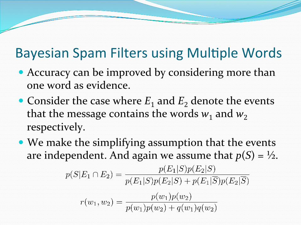
Bayesian Spam Filters using Mul.ple Words � Accuracy can be improved by considering more than one word as evidence.
� Consider the case where E1 and E2 denote the events that the message contains the words w1 and w2 respectively.
� We make the simplifying assumption that the events are independent. And again we assume that p(S) = ½.

Bayesian Spam Filters using Mul.ple Words Example: We have 2000 spam messages and 1000 non-‐spam
messages. The word “stock” occurs in 400 spam messages and in 60 non-‐spam messages. The word “undervalued” occurs in 200 spam
and 25 non-‐spam messages. Should we reject as spam message that contains both “stock” and “undervalued”, if the threshold is set to 0.9?
Solution: p(stock) = 400/2000 = .2, q(stock) = 60/1000=.06, p(undervalued) = 200/2000 = .1, q(undervalued) = 25/1000 = .025
If our threshold is .9, we class the message as spam and reject it.
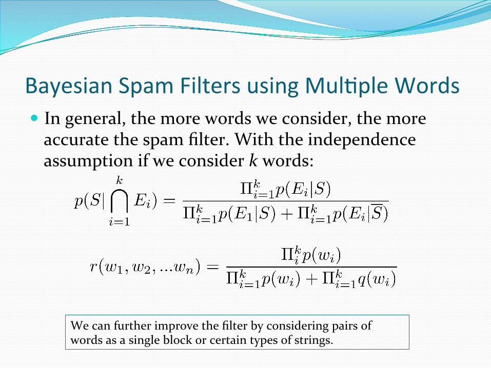
Bayesian Spam Filters using Mul.ple Words � In general, the more words we consider, the more accurate the spam filter. With the independence assumption if we consider k words:
We can further improve the filter by considering pairs of words as a single block or certain types of strings.