Chapter 3

Convex Hull

There exists an incredible variety of point sets and polygons. Among them, some havecertain properties that make them “nicer” than others in some respect. For instance,look at the two polygons shown below.

(a) A convex polygon. (b) A non-convex polygon.

Figure 3.1: Examples of polygons: Which do you like better?

As it is hard to argue about aesthetics, let us take a more algorithmic stance. Whendesigning algorithms, the polygon shown on the left appears much easier to deal withthan the visually and geometrically more complex polygon shown on the right. Oneparticular property that makes the left polygon nice is that one can walk between anytwo vertices along a straight line without ever leaving the polygon. In fact, this statementholds true not only for vertices but for any two points within the polygon. A polygonor, more generally, a set with this property is called convex.

Definition 3.1 A set P ⊆ Rd is convex if pq ⊆ P, for any p,q ∈ P.

An alternative, equivalent way to phrase convexity would be to demand that for everyline ` ⊂ Rd the intersection `∩P be connected. The polygon shown in Figure 3.1b is notconvex because there are some pairs of points for which the connecting line segment is notcompletely contained within the polygon. An immediate consequence of the definitionis the following

16

CG 2013 3.1. Convexity

Observation 3.2 For any family (Pi)i∈I of convex sets, the intersection⋂

i∈I Pi is con-vex.

Indeed there are many problems that are comparatively easy to solve for convex setsbut very hard in general. We will encounter some particular instances of this phenomenonlater in the course. However, not all polygons are convex and a discrete set of points isnever convex, unless it consists of at most one point only. In such a case it is useful tomake a given set P convex, that is, approximate P with or, rather, encompass P withina convex set H ⊇ P. Ideally, H differs from P as little as possible, that is, we want H tobe a smallest convex set enclosing P.

At this point let us step back for a second and ask ourselves whether this wish makessense at all: Does such a set H (always) exist? Fortunately, we are on the safe sidebecause the whole space Rd is certainly convex. It is less obvious, but we will see belowthat H is actually unique. Therefore it is legitimate to refer to H as the smallest convexset enclosing P or—shortly—the convex hull of P.

3.1 Convexity

In this section we will derive an algebraic characterization of convexity. Such a charac-terization allows to investigate convexity using the machinery from linear algebra.

Consider P ⊂ Rd. From linear algebra courses you should know that the linear hull

lin(P) :=q∣∣∣ q =

∑λipi ∧ ∀ i : pi ∈ P, λi ∈ R

is the set of all linear combinations of P (smallest linear subspace containing P). Forinstance, if P = p ⊂ R2 \ 0 then lin(P) is the line through p and the origin.

Similarly, the affine hull

aff(P) :=q∣∣∣ q =

∑λipi ∧

∑λi = 1 ∧ ∀ i : pi ∈ P, λi ∈ R

is the set of all affine combinations of P (smallest affine subspace containing P). Forinstance, if P = p,q ⊂ R2 and p 6= q then aff(P) is the line through p and q.

It turns out that convexity can be described in a very similar way algebraically, whichleads to the notion of convex combinations.

Proposition 3.3 A set P ⊆ Rd is convex if and only if∑n

i=1 λipi ∈ P, for all n ∈ N,p1, . . . ,pn ∈ P, and λ1, . . . , λn > 0 with

∑ni=1 λi = 1.

Proof. “⇐”: obvious with n = 2.“⇒”: Induction on n. For n = 1 the statement is trivial. For n > 2, let pi ∈ P

and λi > 0, for 1 6 i 6 n, and assume∑n

i=1 λi = 1. We may suppose that λi > 0,for all i. (Simply omit those points whose coefficient is zero.) We need to show that∑n

i=1 λipi ∈ P.

17

Chapter 3. Convex Hull CG 2013

Define λ =∑n−1

i=1 λi and for 1 6 i 6 n − 1 set µi = λi/λ. Observe that µi > 0and

∑n−1i=1 µi = 1. By the inductive hypothesis, q :=

∑n−1i=1 µipi ∈ P, and thus by

convexity of P also λq + (1 − λ)pn ∈ P. We conclude by noting that λq + (1 − λ)pn =λ∑n−1

i=1 µipi + λnpn =∑n

i=1 λipi.

Definition 3.4 The convex hull conv(P) of a set P ⊆ Rd is the intersection of all convexsupersets of P.

At first glance this definition is a bit scary: There may be a whole lot of supersets forany given P and it not clear that taking the intersection of all of them yields somethingsensible to work with. However, by Observation 3.2 we know that the resulting setis convex, at least. The missing bit is provided by the following proposition, whichcharacterizes the convex hull in terms of exactly those convex combinations that appearedin Proposition 3.3 already.

Proposition 3.5 For any P ⊆ Rd we have

conv(P) =

n∑

i=1

λipi

∣∣∣∣∣ n ∈ N ∧

n∑i=1

λi = 1 ∧ ∀i ∈ 1, . . . ,n : λi > 0∧ pi ∈ P

.

The elements of the set on the right hand side are referred to as convex combinationsof P.Proof. “⊇”: Consider a convex set C ⊇ P. By Proposition 3.3 (only-if direction) theright hand side is contained in C. As C was arbitrary, the claim follows.

“⊆”: Denote the set on the right hand side by R. Clearly R ⊇ P. We show that Rforms a convex set. Let p =

∑ni=1 λipi and q =

∑ni=1 µipi be two convex combinations.

(We may suppose that both p and q are expressed over the same pi by possibly addingsome terms with a coefficient of zero.)

Then for λ ∈ [0, 1] we have λp + (1 − λ)q =∑n

i=1(λλi + (1 − λ)µi)pi ∈ R, asλλi︸︷︷︸>0

+(1− λ)︸ ︷︷ ︸>0

µi︸︷︷︸>0

> 0, for all 1 6 i 6 n, and∑n

i=1(λλi+(1−λ)µi) = λ+(1−λ) = 1.

In linear algebra the notion of a basis in a vector space plays a fundamental role. Ina similar way we want to describe convex sets using as few entities as possible, whichleads to the notion of extremal points, as defined below.

Definition 3.6 The convex hull of a finite point set P ⊂ Rd forms a convex polytope.Each p ∈ P for which p /∈ conv(P \ p) is called a vertex of conv(P). A vertex ofconv(P) is also called an extremal point of P. A convex polytope in R2 is called aconvex polygon.

Essentially, the following proposition shows that the term vertex above is well defined.

Proposition 3.7 A convex polytope in Rd is the convex hull of its vertices.

18

CG 2013 3.2. Classical Theorems for Convex Sets

Proof. Let P = p1, . . . ,pn, n ∈ N, such that without loss of generality p1, . . . ,pkare the vertices of P := conv(P). We prove by induction on n that conv(p1, . . . ,pn) ⊆conv(p1, . . . ,pk). For n = k the statement is trivial.

For n > k, pn is not a vertex of P and hence pn can be expressed as a convexcombination pn =

∑n−1i=1 λipi. Thus for any x ∈ P we can write x =

∑ni=1 µipi =∑n−1

i=1 µipi+µn

∑n−1i=1 λipi =

∑n−1i=1 (µi+µnλi)pi. As

∑n−1i=1 (µi+µnλi) = 1, we conclude

inductively that x ∈ conv(p1, . . . ,pn−1) ⊆ conv(p1, . . . ,pk).

3.2 Classical Theorems for Convex Sets

Next we will discuss a few fundamental theorems about convex sets in Rd. The proofstypically use the algebraic characterization of convexity and then employ some techniquesfrom linear algebra.

Theorem 3.8 (Radon [8]) Any set P ⊂ Rd of d + 2 points can be partitioned into twodisjoint subsets P1 and P2 such that conv(P1) ∩ conv(P2) 6= ∅.

Proof. Let P = p1, . . . ,pd+2. No more than d + 1 points can be affinely independentin Rd. Hence suppose without loss of generality that pd+2 can be expressed as an affinecombination of p1, . . . ,pd+1, that is, there exist λ1, . . . , λd+1 ∈ R with

∑d+1i=1 λi = 1

and∑d+1

i=1 λipi = pd+2. Let P1 be the set of all points pi for which λi is positive andlet P2 = P \ P1. Then setting λd+2 = −1 we can write

∑pi∈P1

λipi =∑

pi∈P2−λipi,

where all coefficients on both sides are non-negative. Renormalizing by µi = λi/µ andνi = λi/ν, where µ =

∑pi∈P1

λi and ν = −∑

pi∈P2λi, yields convex combinations∑

pi∈P1µipi =

∑pi∈P2

νipi that describe a common point of conv(P1) and conv(P2).

Theorem 3.9 (Helly) Consider a collection C = C1, . . . ,Cn of n > d+1 convex subsetsof Rd, such that any d+1 pairwise distinct sets from C have non-empty intersection.Then also the intersection

⋂ni=1Ci of all sets from C is non-empty.

Proof. Induction on n. The base case n = d + 1 holds by assumption. Hence supposethat n > d + 2. Consider the sets Di =

⋂j6=iCj, for i ∈ 1, . . . ,n. As Di is an

intersection of n − 1 sets from C, by the inductive hypothesis we know that Di 6= ∅.Therefore we can find some point pi ∈ Di, for each i ∈ 1, . . . ,n. Now by Theorem 3.8the set P = p1, . . . ,pn can be partitioned into two disjoint subsets P1 and P2 such thatconv(P1) ∩ conv(P2) 6= ∅. We claim that any point p ∈ conv(P1) ∩ conv(P2) also lies in⋂n

i=1Ci, which completes the proof.Consider some Ci, for i ∈ 1, . . . ,n. By construction Dj ⊆ Ci, for j 6= i. Thus pi

is the only point from P that may not be in Ci. As pi is part of only one of P1 or P2,say, of P1, we have P2 ⊆ Ci. The convexity of Ci implies conv(P2) ⊆ Ci and, therefore,p ∈ Ci.

19

Chapter 3. Convex Hull CG 2013

Theorem 3.10 (Carathéodory [3]) For any P ⊂ Rd and q ∈ conv(P) there exist k 6 d+ 1points p1, . . . ,pk ∈ P such that q ∈ conv(p1, . . . ,pk).

Exercise 3.11 Prove Theorem 3.10.

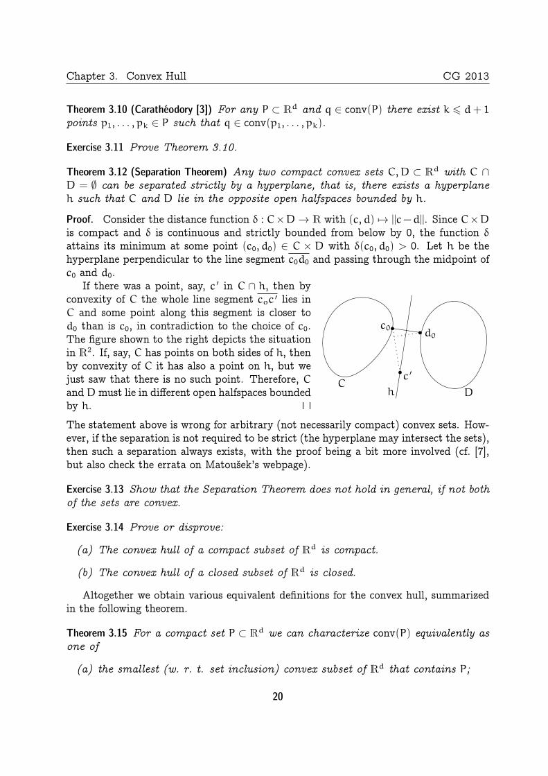
Theorem 3.12 (Separation Theorem) Any two compact convex sets C,D ⊂ Rd with C ∩D = ∅ can be separated strictly by a hyperplane, that is, there exists a hyperplaneh such that C and D lie in the opposite open halfspaces bounded by h.

Proof. Consider the distance function δ : C×D→ R with (c,d) 7→ ||c−d||. Since C×Dis compact and δ is continuous and strictly bounded from below by 0, the function δattains its minimum at some point (c0,d0) ∈ C × D with δ(c0,d0) > 0. Let h be thehyperplane perpendicular to the line segment c0d0 and passing through the midpoint ofc0 and d0.

c0d0

CDh

c ′

If there was a point, say, c ′ in C ∩ h, then byconvexity of C the whole line segment coc ′ lies inC and some point along this segment is closer tod0 than is c0, in contradiction to the choice of c0.The figure shown to the right depicts the situationin R2. If, say, C has points on both sides of h, thenby convexity of C it has also a point on h, but wejust saw that there is no such point. Therefore, CandDmust lie in different open halfspaces boundedby h.

The statement above is wrong for arbitrary (not necessarily compact) convex sets. How-ever, if the separation is not required to be strict (the hyperplane may intersect the sets),then such a separation always exists, with the proof being a bit more involved (cf. [7],but also check the errata on Matoušek’s webpage).

Exercise 3.13 Show that the Separation Theorem does not hold in general, if not bothof the sets are convex.

Exercise 3.14 Prove or disprove:

(a) The convex hull of a compact subset of Rd is compact.

(b) The convex hull of a closed subset of Rd is closed.

Altogether we obtain various equivalent definitions for the convex hull, summarizedin the following theorem.

Theorem 3.15 For a compact set P ⊂ Rd we can characterize conv(P) equivalently asone of

(a) the smallest (w. r. t. set inclusion) convex subset of Rd that contains P;

20

CG 2013 3.3. Planar Convex Hull

(b) the set of all convex combinations of points from P;

(c) the set of all convex combinations formed by d+ 1 or fewer points from P;

(d) the intersection of all convex supersets of P;

(e) the intersection of all closed halfspaces containing P.

Exercise 3.16 Prove Theorem 3.15.

3.3 Planar Convex Hull

Although we know by now what is the convex hull of point set, it is not yet clear howto construct it algorithmically. As a first step, we have to find a suitable representationfor convex hulls. In this section we focus on the problem in R2, where the convex hullof a finite point set forms a convex polygon. A convex polygon is easy to represent,for instance, as a sequence of its vertices in counterclockwise orientation. In higherdimensions finding a suitable representation for convex polytopes is a much more delicatetask.

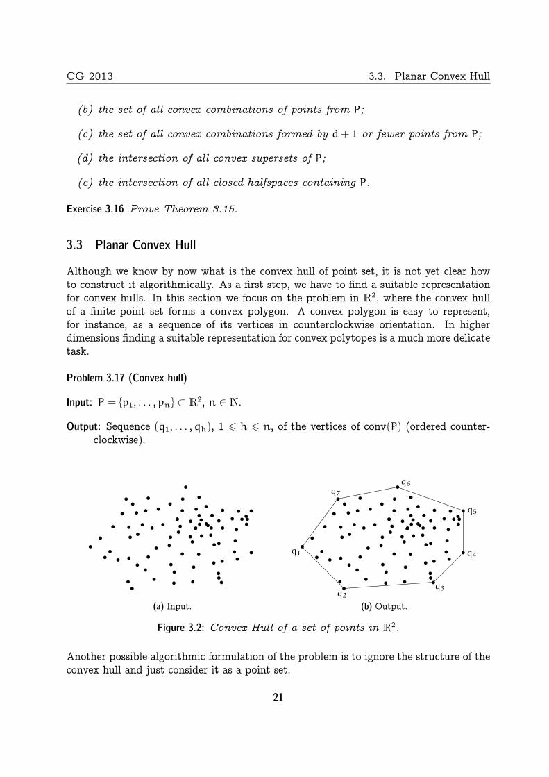
Problem 3.17 (Convex hull)

Input: P = p1, . . . ,pn ⊂ R2, n ∈ N.

Output: Sequence (q1, . . . ,qh), 1 6 h 6 n, of the vertices of conv(P) (ordered counter-clockwise).

q1

q2

q3

q4

q5

q6

q7

(a) Input.

q1

q2

q3

q4

q5

q6

q7

(b) Output.

Figure 3.2: Convex Hull of a set of points in R2.

Another possible algorithmic formulation of the problem is to ignore the structure of theconvex hull and just consider it as a point set.

21

Chapter 3. Convex Hull CG 2013

Problem 3.18 (Extremal points)

Input: P = p1, . . . ,pn ⊂ R2, n ∈ N.

Output: Set Q ⊆ P of the vertices of conv(P).

Degeneracies. A couple of further clarifications regarding the above problem definitionsare in order.

First of all, for efficiency reasons an input is usually specified as a sequence of points.Do we insist that this sequence forms a set or are duplications of points allowed?

What if three points are collinear? Are all of them considered extremal? Accordingto our definition from above, they are not and that is what we will stick to. But notethat there may be cases where one wants to include all such points, nevertheless.

By the Separation Theorem, every extremal point p can be separated from the convexhull of the remaining points by a halfplane. If we take such a halfplane and translate itsdefining line such that it passes through p, then all points from P other than p should liein the resulting open halfplane. In R2 it turns out convenient to work with the following“directed” reformulation.

Proposition 3.19 A point p ∈ P = p1, . . . ,pn ⊂ R2 is extremal for P ⇐⇒ there is adirected line g through p such that P \ p is to the left of g.

cr

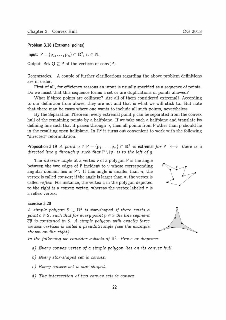
The interior angle at a vertex v of a polygon P is the anglebetween the two edges of P incident to v whose correspondingangular domain lies in P. If this angle is smaller than π, thevertex is called convex ; if the angle is larger than π, the vertex iscalled reflex. For instance, the vertex c in the polygon depictedto the right is a convex vertex, whereas the vertex labeled r isa reflex vertex.

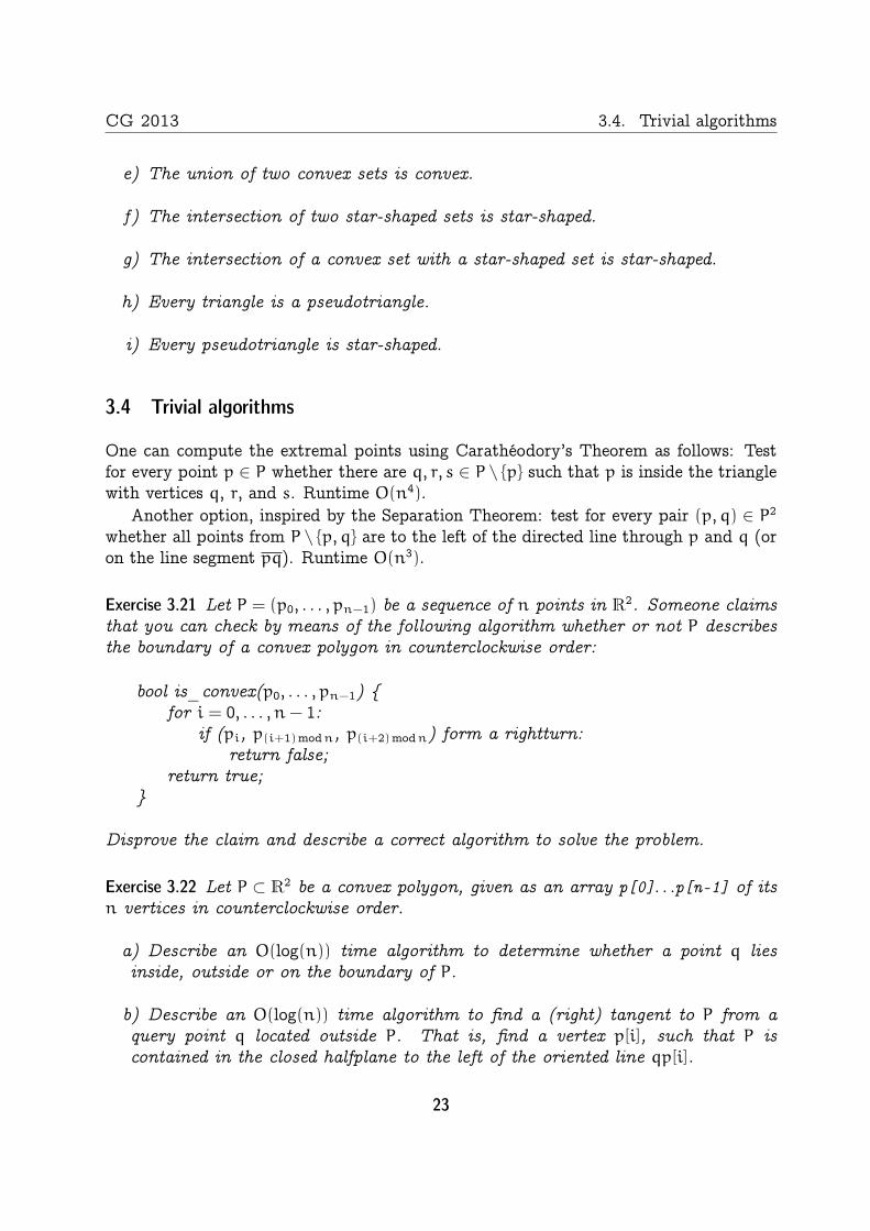
Exercise 3.20A simple polygon S ⊂ R2 is star-shaped if there exists apoint c ∈ S, such that for every point p ∈ S the line segmentcp is contained in S. A simple polygon with exactly threeconvex vertices is called a pseudotriangle (see the exampleshown on the right).In the following we consider subsets of R2. Prove or disprove:

a) Every convex vertex of a simple polygon lies on its convex hull.

b) Every star-shaped set is convex.

c) Every convex set is star-shaped.

d) The intersection of two convex sets is convex.

22

CG 2013 3.4. Trivial algorithms

e) The union of two convex sets is convex.

f) The intersection of two star-shaped sets is star-shaped.

g) The intersection of a convex set with a star-shaped set is star-shaped.

h) Every triangle is a pseudotriangle.

i) Every pseudotriangle is star-shaped.

3.4 Trivial algorithms

One can compute the extremal points using Carathéodory’s Theorem as follows: Testfor every point p ∈ P whether there are q, r, s ∈ P \ p such that p is inside the trianglewith vertices q, r, and s. Runtime O(n4).

Another option, inspired by the Separation Theorem: test for every pair (p,q) ∈ P2

whether all points from P \ p,q are to the left of the directed line through p and q (oron the line segment pq). Runtime O(n3).

Exercise 3.21 Let P = (p0, . . . ,pn−1) be a sequence of n points in R2. Someone claimsthat you can check by means of the following algorithm whether or not P describesthe boundary of a convex polygon in counterclockwise order:

bool is_convex(p0, . . . ,pn−1) for i = 0, . . . ,n− 1:

if (pi, p(i+1)modn, p(i+2)modn) form a rightturn:return false;

return true;

Disprove the claim and describe a correct algorithm to solve the problem.

Exercise 3.22 Let P ⊂ R2 be a convex polygon, given as an array p[0]. . .p[n-1] of itsn vertices in counterclockwise order.

a) Describe an O(log(n)) time algorithm to determine whether a point q liesinside, outside or on the boundary of P.

b) Describe an O(log(n)) time algorithm to find a (right) tangent to P from aquery point q located outside P. That is, find a vertex p[i], such that P iscontained in the closed halfplane to the left of the oriented line qp[i].

23

Chapter 3. Convex Hull CG 2013

3.5 Jarvis’ Wrap

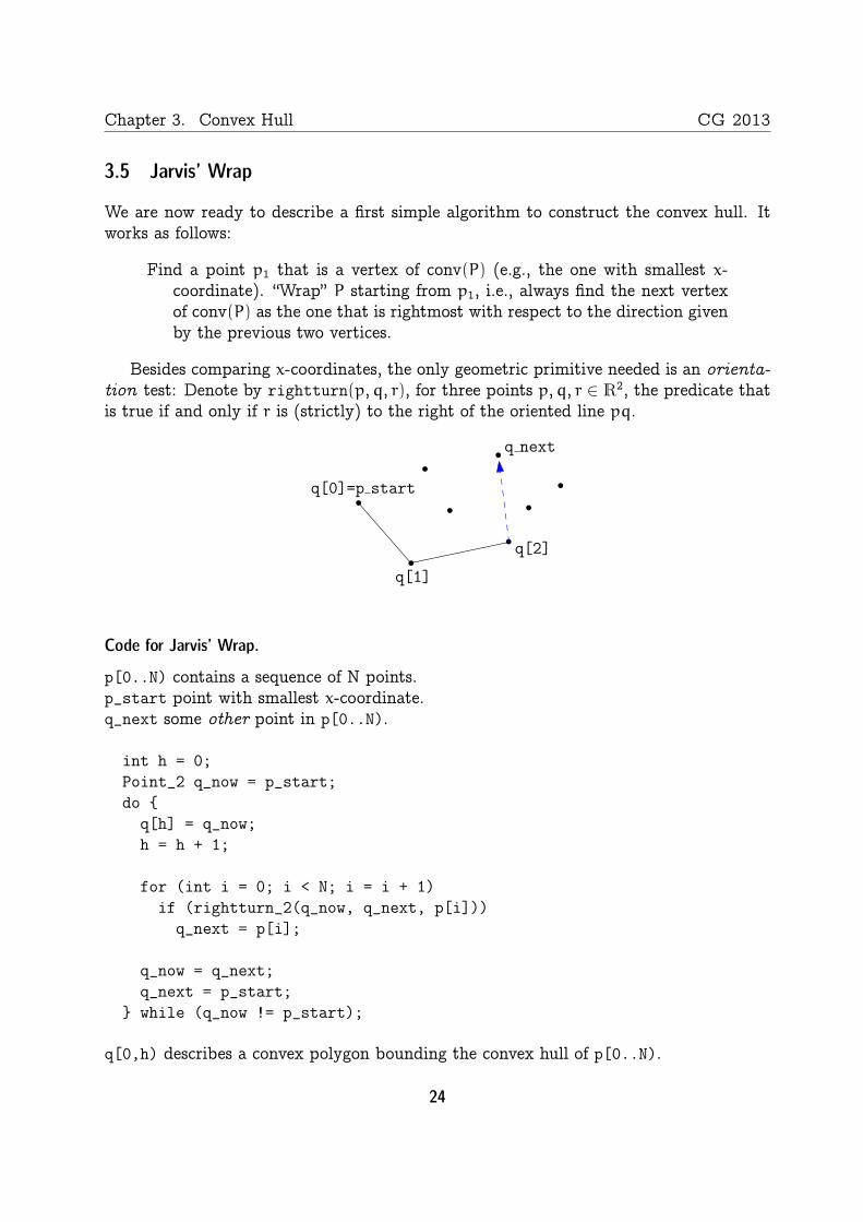
We are now ready to describe a first simple algorithm to construct the convex hull. Itworks as follows:

Find a point p1 that is a vertex of conv(P) (e.g., the one with smallest x-coordinate). “Wrap” P starting from p1, i.e., always find the next vertexof conv(P) as the one that is rightmost with respect to the direction givenby the previous two vertices.

Besides comparing x-coordinates, the only geometric primitive needed is an orienta-tion test: Denote by rightturn(p,q, r), for three points p,q, r ∈ R2, the predicate thatis true if and only if r is (strictly) to the right of the oriented line pq.

q[0]=p start

q next

q[1]

q[2]

Code for Jarvis’ Wrap.

p[0..N) contains a sequence of N points.p_start point with smallest x-coordinate.q_next some other point in p[0..N).

int h = 0;Point_2 q_now = p_start;do

q[h] = q_now;h = h + 1;

for (int i = 0; i < N; i = i + 1)if (rightturn_2(q_now, q_next, p[i]))

q_next = p[i];

q_now = q_next;q_next = p_start;

while (q_now != p_start);

q[0,h) describes a convex polygon bounding the convex hull of p[0..N).

24

CG 2013 3.5. Jarvis’ Wrap

Analysis. For every output point the above algorithm spends n rightturn tests, which is⇒ O(nh) in total.

Theorem 3.23 [6] Jarvis’ Wrap computes the convex hull of n points in R2 usingO(nh) rightturn tests, where h is the number of hull vertices.

In the worst case we have h = n, that is, O(n2) rightturn tests. Jarvis’ Wrap has aremarkable property that is called output sensitivity : the runtime depends not only onthe size of the input but also on the size of the output. For a huge point set it constructsthe convex hull in optimal linear time, if the convex hull consists of a constant number ofvertices only. Unfortunately the worst case performance of Jarvis’ Wrap is suboptimal,as we will see soon.

Degeneracies. The algorithm may have to cope with various degeneracies.

Several points have smallest x-coordinate ⇒ lexicographic order:

(px,py) < (qx,qy) ⇐⇒ px < qx ∨ px = qx ∧ py < qy .

Three or more points collinear ⇒ choose the point that is farthest among thosethat are rightmost.

Predicates. Besides the lexicographic comparison mentioned above, the Jarvis’ Wrap(and most other 2D convex hull algorithms for that matter) need one more geomet-ric predicate: the rightturn or—more generally—orientation test. The computationamounts to evaluating a polynomial of degree two, see the exercise below. We thereforesay that the orientation test has algebraic degree two. In contrast, the lexicographiccomparison has degree one only. The algebraic degree not only has a direct impact onthe efficiency of a geometric algorithm (lower degree↔ less multiplications), but also anindirect one because high degree predicates may create large intermediate results, whichmay lead to overflows and are much more costly to compute with exactly.

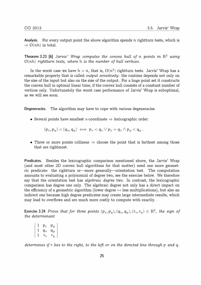
Exercise 3.24 Prove that for three points (px,py), (qx,qy), (rx, ry) ∈ R2, the sign ofthe determinant∣∣∣∣∣∣

1 px py1 qx qy

1 rx ry

∣∣∣∣∣∣determines if r lies to the right, to the left or on the directed line through p and q.

25

Chapter 3. Convex Hull CG 2013

3.6 Graham Scan (Successive Local Repair)

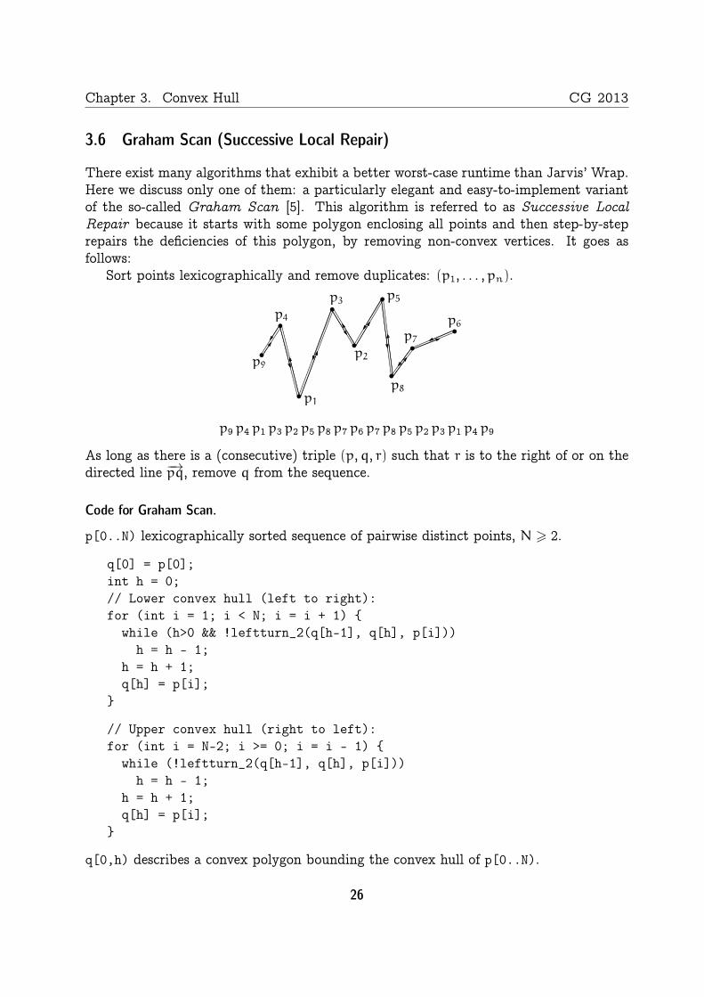
There exist many algorithms that exhibit a better worst-case runtime than Jarvis’ Wrap.Here we discuss only one of them: a particularly elegant and easy-to-implement variantof the so-called Graham Scan [5]. This algorithm is referred to as Successive LocalRepair because it starts with some polygon enclosing all points and then step-by-steprepairs the deficiencies of this polygon, by removing non-convex vertices. It goes asfollows:

Sort points lexicographically and remove duplicates: (p1, . . . ,pn).

p9

p4

p1

p3

p2

p5

p8

p7

p6

p9 p4 p1 p3 p2 p5 p8 p7 p6 p7 p8 p5 p2 p3 p1 p4 p9

As long as there is a (consecutive) triple (p,q, r) such that r is to the right of or on thedirected line −→pq, remove q from the sequence.

Code for Graham Scan.

p[0..N) lexicographically sorted sequence of pairwise distinct points, N > 2.

q[0] = p[0];int h = 0;// Lower convex hull (left to right):for (int i = 1; i < N; i = i + 1)

while (h>0 && !leftturn_2(q[h-1], q[h], p[i]))h = h - 1;

h = h + 1;q[h] = p[i];

// Upper convex hull (right to left):for (int i = N-2; i >= 0; i = i - 1)

while (!leftturn_2(q[h-1], q[h], p[i]))h = h - 1;

h = h + 1;q[h] = p[i];

q[0,h) describes a convex polygon bounding the convex hull of p[0..N).

26

CG 2013 3.7. Lower Bound

Analysis.

Theorem 3.25 The convex hull of a set P ⊂ R2 of n points can be computed usingO(n logn) geometric operations.

Proof.

1. Sorting and removal of duplicate points: O(n logn).

2. At the beginning we have a sequence of 2n − 1 points; at the end the sequenceconsists of h points. Observe that for every positive orientation test, one point isdiscarded from the sequence for good. Therefore, we have exactly 2n− h− 1 suchshortcuts/positive orientation tests. In addition there are at most 2n− 2 negativetests (#iterations of the outer for loops). Altogether we have at most 4n− h− 3orientation tests.

In total the algorithm uses O(n logn) geometric operations. Note that the number oforientation tests is linear only, but O(n logn) lexicographic comparisons are needed.

3.7 Lower Bound

It is not hard to see that the runtime of Graham Scan is asymptotically optimal in theworst-case.

Theorem 3.26 Ω(n logn) geometric operations are needed to construct the convex hullof n points in R2 (in the algebraic computation tree model).

Proof. Reduction from sorting (for which it is known that Ω(n logn) comparisonsare needed in the algebraic computation tree model). Given n real numbers x1, . . . , xn,construct a set P = pi | 1 6 i 6 n of n points in R2 by setting pi = (xi, x2

i). Thisconstruction can be regarded as embedding the numbers into R2 along the x-axis andthen projecting the resulting points vertically onto the unit parabola. The order in whichthe points appear along the lower convex hull of P corresponds to the sorted order ofthe xi. Therefore, if we could construct the convex hull in o(n logn) time, we could alsosort in o(n logn) time.

Clearly this reduction does not work for the Extremal Points problem. But us-ing a reduction from Element Uniqueness (see Section 1.1) instead, one can show thatΩ(n logn) is also a lower bound for the number of operations needed to compute the setof extremal points only. This was first shown by Avis [1] for linear computation trees,then by Yao [9] for quadratic computation trees, and finally by Ben-Or [2] for generalalgebraic computation trees.

27

Chapter 3. Convex Hull CG 2013

3.8 Chan’s Algorithm

Given matching upper and lower bounds we may be tempted to consider the algorithmiccomplexity of the planar convex hull problem settled. However, this is not really thecase: Recall that the lower bound is a worst case bound. For instance, the Jarvis’ Wrapruns in O(nh) time an thus beats the Ω(n logn) bound in case that h = o(logn). Thequestion remains whether one can achieve both output dependence and optimal worstcase performance at the same time. Indeed, Chan [4] presented an algorithm to achievethis runtime by cleverly combining the “best of” Jarvis’ Wrap and Graham Scan. Let uslook at this algorithm in detail. The algorithm consists of two steps that are executedone after another.

Divide. Input: a set P ⊂ R2 of n points and a number H ∈ 1, . . . ,n.

1. Divide P into k = dn/He sets P1, . . . ,Pk with |Pi| 6 H.

2. Construct conv(Pi) for all i, 1 6 i 6 k.

Analysis. Step 1 takes O(n) time. Step 2 can be handled using Graham Scan inO(H logH) time for any single Pi, that is, O(n logH) time in total.

Conquer. Output: the vertices of conv(P) in counterclockwise order, if conv(P) has lessthan H vertices; otherwise, the message that conv(P) has at least H vertices.

1. Find the lexicographically smallest point in conv(Pi) for all i, 1 6 i 6 k.

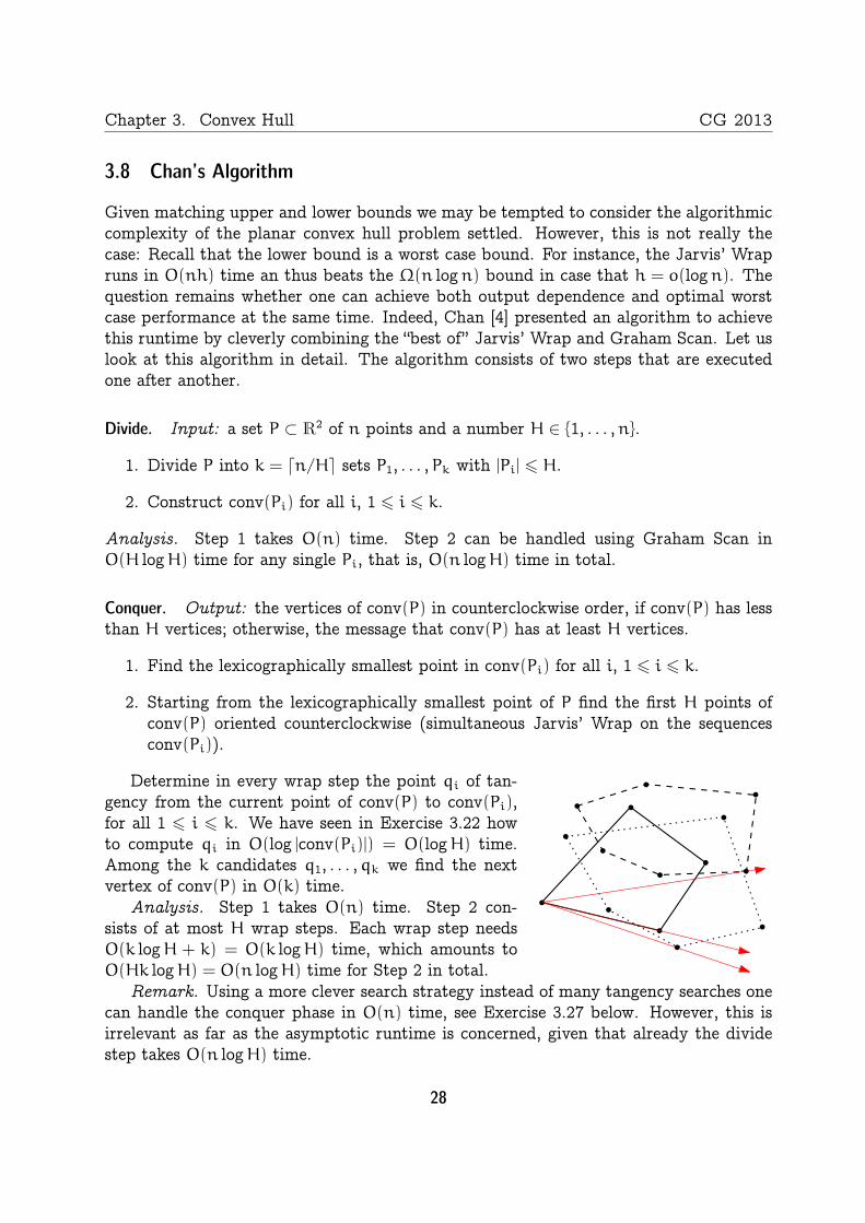
2. Starting from the lexicographically smallest point of P find the first H points ofconv(P) oriented counterclockwise (simultaneous Jarvis’ Wrap on the sequencesconv(Pi)).

Determine in every wrap step the point qi of tan-gency from the current point of conv(P) to conv(Pi),for all 1 6 i 6 k. We have seen in Exercise 3.22 howto compute qi in O(log |conv(Pi)|) = O(logH) time.Among the k candidates q1, . . . ,qk we find the nextvertex of conv(P) in O(k) time.

Analysis. Step 1 takes O(n) time. Step 2 con-sists of at most H wrap steps. Each wrap step needsO(k logH + k) = O(k logH) time, which amounts toO(Hk logH) = O(n logH) time for Step 2 in total.

Remark. Using a more clever search strategy instead of many tangency searches onecan handle the conquer phase in O(n) time, see Exercise 3.27 below. However, this isirrelevant as far as the asymptotic runtime is concerned, given that already the dividestep takes O(n logH) time.

28

CG 2013 3.8. Chan’s Algorithm

Exercise 3.27 Consider k convex polygons P1, . . .Pk, for some constant k ∈ N, whereeach polygon is given as a list of its vertices in counterclockwise orientation. Showhow to construct the convex hull of P1 ∪ . . . ∪ Pk in O(n) time, where n =

∑ki=1 ni

and ni is the number of vertices of Pi, for 1 6 i 6 k.

Searching for h. While the runtime bound for H = h is exactly what we were heading for,it looks like in order to actually run the algorithm we would have to know h, which—in general—we do not. Fortunately we can circumvent this problem rather easily, byapplying what is called a doubly exponential search. It works as follows.

Call the algorithm from above iteratively with parameter H = min22t ,n, for t =0, . . ., until the conquer step finds all extremal points of P (i.e., the wrap returns to itsstarting point).

Analysis: Let 22s be the last parameter for which the algorithm is called. Since theprevious call with H = 22s−1 did not find all extremal points, we know that 22s−1

< h,that is, 2s−1 < logh, where h is the number of extremal points of P. The total runtimeis therefore at most

s∑i=0

cn log 22i = cn

s∑i=0

2i = cn(2s+1 − 1) < 4cn logh = O(n logh),

for some constant c ∈ R. In summary, we obtain the following theorem.

Theorem 3.28 The convex hull of a set P ⊂ R2 of n points can be computed usingO(n logh) geometric operations, where h is the number of convex hull vertices.

Questions

6. How is convexity defined? What is the convex hull of a set in Rd? Give atleast three possible definitions.

7. What does it mean to compute the convex hull of a set of points in R2? Discussinput and expected output and possible degeneracies.

8. How can the convex hull of a set of n points in R2 be computed efficiently?Describe and analyze (incl. proofs) Jarvis’ Wrap, Successive Local Repair, andChan’s Algorithm.

9. Is there a linear time algorithm to compute the convex hull of n points in R2?Prove the lower bound and define/explain the model in which it holds.

10. Which geometric primitive operations are used to compute the convex hull ofn points in R2? Explain the two predicates and how to compute them.

29

Chapter 3. Convex Hull CG 2013

Remarks. The sections on Jarvis’ Wrap and Graham Scan are based on material thatEmo Welzl prepared for a course on “Geometric Computing” in 2000.

References

[1] David Avis, Comments on a lower bound for convex hull determination. Inform. Pro-cess. Lett., 11, 3, (1980), 126, URL http://dx.doi.org/10.1016/0020-0190(80)90125-8.

[2] Michael Ben-Or, Lower bounds for algebraic computation trees. In Proc. 15th Annu.ACM Sympos. Theory Comput., pp. 80–86, 1983, URL http://dx.doi.org/10.1145/800061.808735.

[3] Constantin Carathéodory, Über den Variabilitätsbereich der Fourierschen Konstan-ten von positiven harmonischen Funktionen. Rendiconto del Circolo Matematicodi Palermo, 32, (1911), 193–217, URL http://dx.doi.org/10.1007/BF03014795.

[4] Timothy M. Chan, Optimal output-sensitive convex hull algorithms in two and threedimensions. Discrete Comput. Geom., 16, 4, (1996), 361–368, URL http://dx.doi.org/10.1007/BF02712873.

[5] Ronald L. Graham, An efficient algorithm for determining the convex hull of a finiteplanar set. Inform. Process. Lett., 1, 4, (1972), 132–133, URL http://dx.doi.org/10.1016/0020-0190(72)90045-2.

[6] Ray A. Jarvis, On the identification of the convex hull of a finite set of points inthe plane. Inform. Process. Lett., 2, 1, (1973), 18–21, URL http://dx.doi.org/10.1016/0020-0190(73)90020-3.

[7] Jiří Matoušek, Lectures on discrete geometry. Springer-Verlag, New York, NY, 2002.

[8] Johann Radon, Mengen konvexer Körper, die einen gemeinsamen Punkt enthal-ten. Math. Annalen, 83, 1–2, (1921), 113–115, URL http://dx.doi.org/10.1007/BF01464231.

[9] Andrew C. Yao, A lower bound to finding convex hulls. J. ACM, 28, 4, (1981),780–787, URL http://dx.doi.org/10.1145/322276.322289.

30