Chapter VII Wave Statistics & Wave Spectra

Previously, the regular waves (signle frequency and amplitude) have been studied.

However, ocean waves are almost irregular.

7.1 Introduction

1. How to use wave statistics and wave to describe (or simulate) irregular waves.

2. How to use the previous knowledge based on (regular) linear wave theory to calculate the properties of irregular waves.

3. Wave Statistics4. Wave Spectra5. FFT (decompose) and IFFT (superposition or simulation)

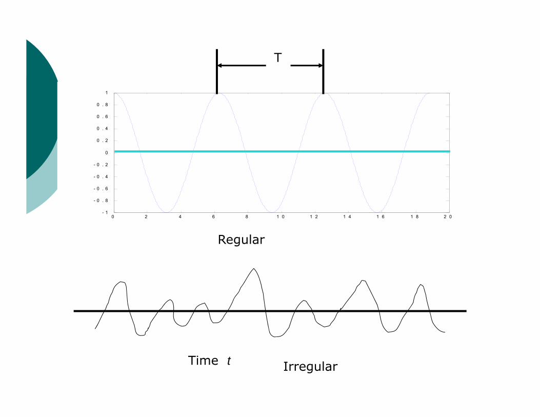
Regular and Irregular Waves

Ocean waves are almost always irregular or random.

Irregular waves can be viewed as the superposition of a number of regular waves (wave components) with different frequencies and amplitudes.

A regular wave (wave component) has a single frequency (wavelength) and amplitude (height).

Irregular Waves: long-crested & short-crested

All wave components are in the same direction ---- Uni-directionalirregular waves, aka, long-crested irregular waves.

Wave components are often multi-directional, ---- directional irregular waves, aka, short-crested waves.

0 2 4 6 8 1 0 1 2 1 4 1 6 1 8 2 0- 1

- 0 . 8

- 0 . 6

- 0 . 4

- 0 . 2

0

0 . 2

0 . 4

0 . 6

0 . 8

1

T

Time t

Regular

Irregular

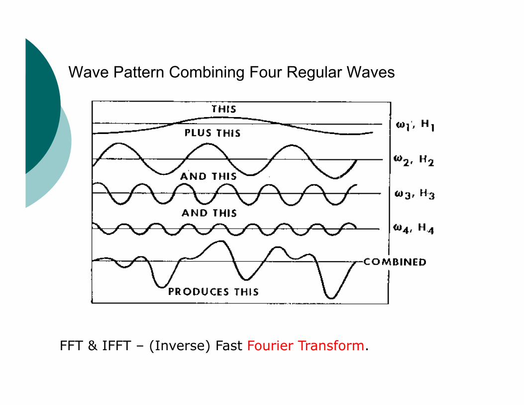
Wave Pattern Combining Four Regular Waves

FFT & IFFT – (Inverse) Fast Fourier Transform.

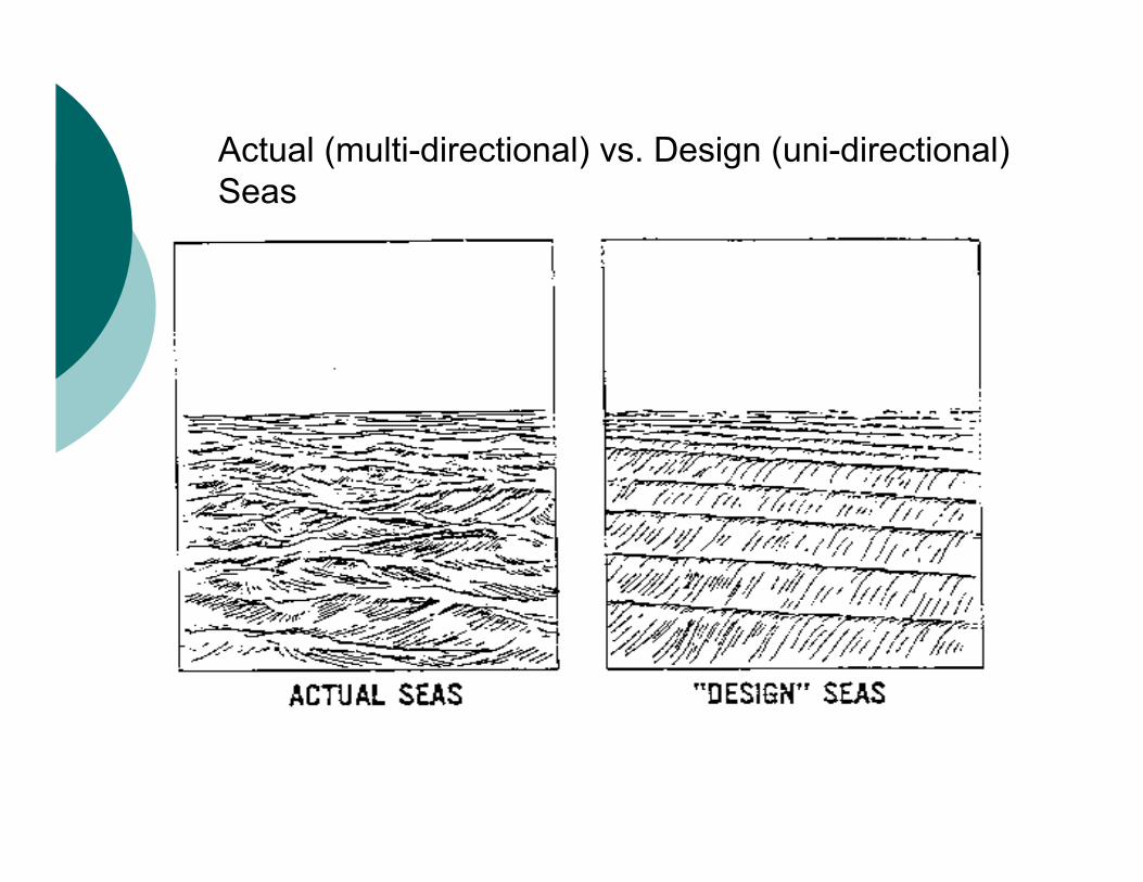
Actual (multi-directional) vs. Design (uni-directional) Seas

7.2 Wave Height Distribution

Different from a regular wave train, in an irregular wave train, wave heights and wave periods are not uniform

How to count the wave heights and wave periods in an irregular wave train.

Zero up-crossing and zero down-crossing method.

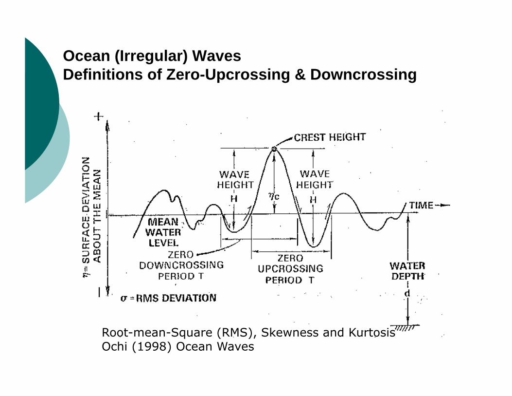
Ocean (Irregular) Waves Definitions of Zero-Upcrossing & Downcrossing

Root-mean-Square (RMS), Skewness and Kurtosis Ochi (1998) Ocean Waves

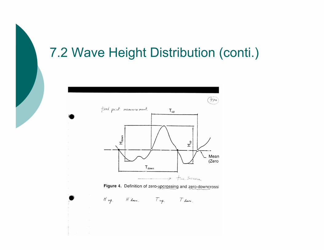
7.2 Wave Height Distribution (conti.)

Probability Density Function (PDF)

Probability density function (pdf), is a function that describes the relative likelihood for this random variable to take on a given value. The probability for the random variable to fall within a particular region is given by the integral of this variable’s density over the region. The probability density function is nonnegative everywhere, and its integral over the entire space is equal to one.

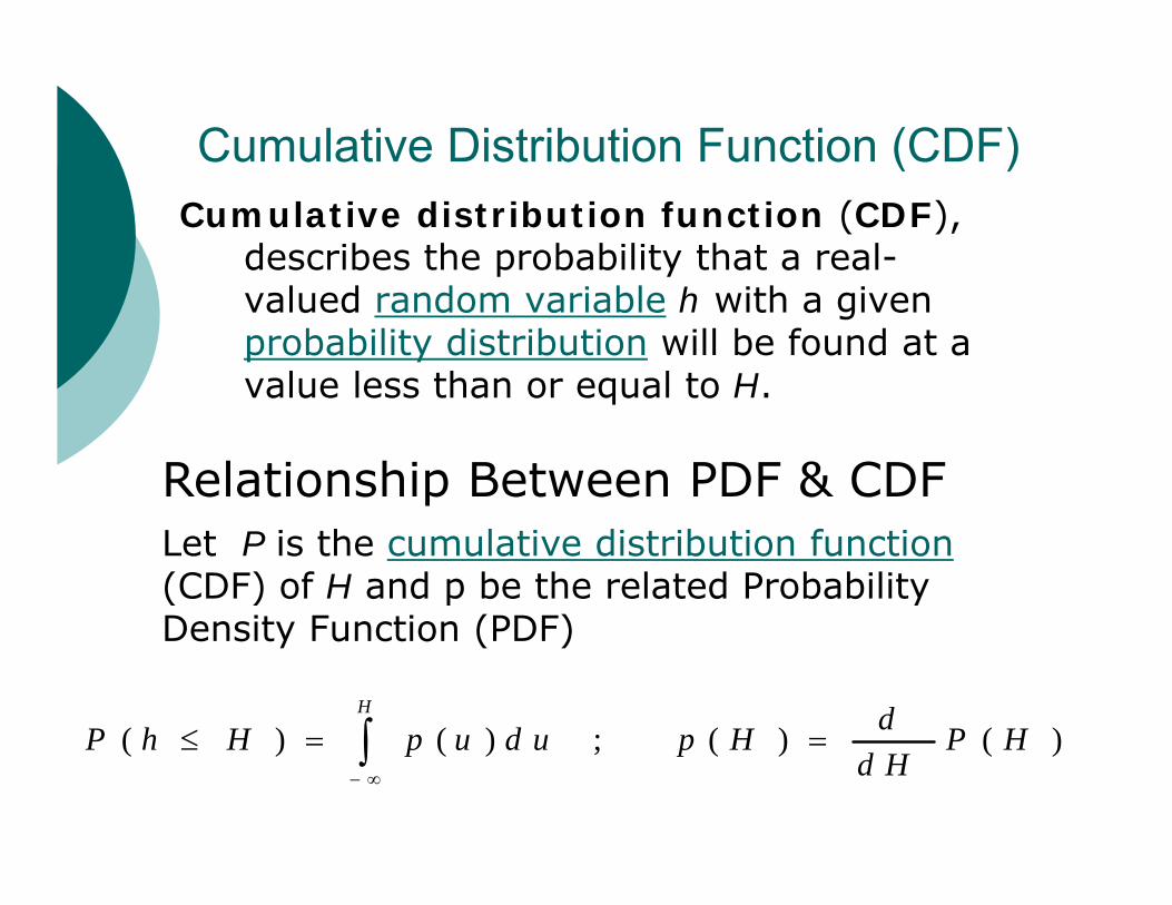
Cumulative Distribution Function (CDF)Cumulative distribution function (CDF),

describes the probability that a real-valued random variable h with a given probability distribution will be found at a value less than or equal to H.

Relationship Between PDF & CDFLet P is the cumulative distribution function(CDF) of H and p be the related Probability Density Function (PDF)

( ) ( ) ; ( ) ( )H dP h H p u d u p H P H

d H

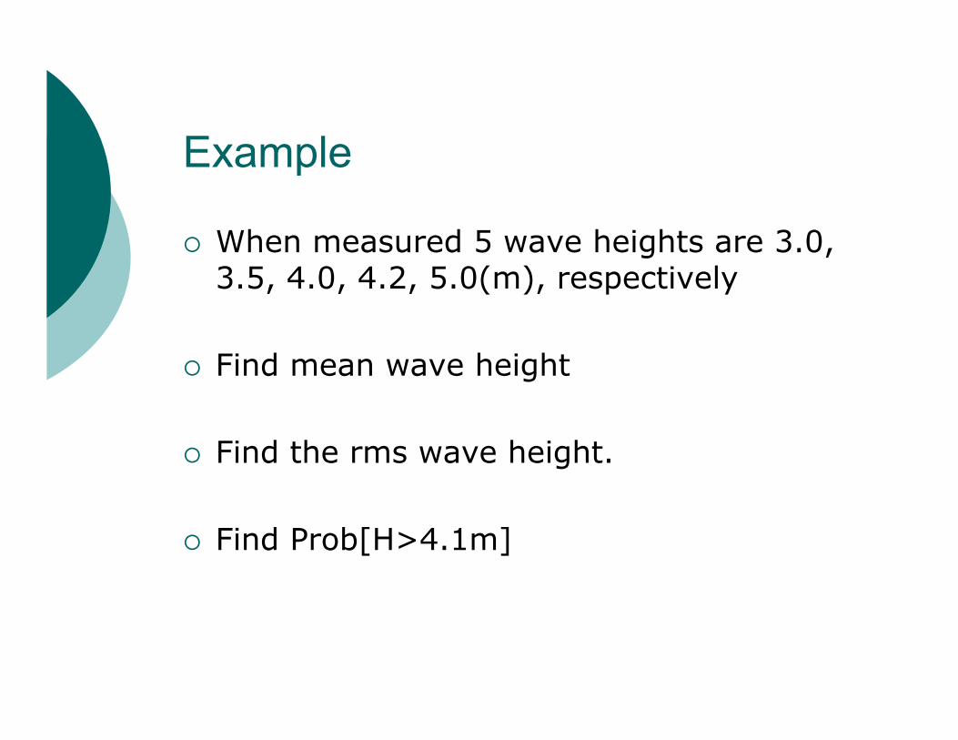
Example

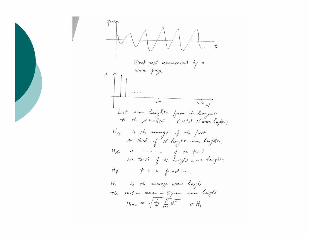
When measured 5 wave heights are 3.0, 3.5, 4.0, 4.2, 5.0(m), respectively

Find mean wave height

Find the rms wave height.

Find Prob[H>4.1m]

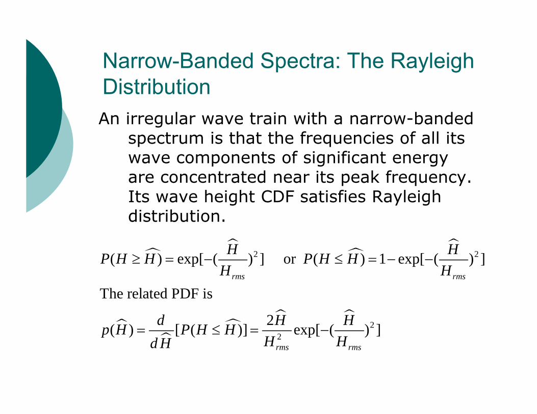
Narrow-Banded Spectra: The RayleighDistributionAn irregular wave train with a narrow-banded

spectrum is that the frequencies of all its wave components of significant energy are concentrated near its peak frequency. Its wave height CDF satisfies Rayleigh distribution.

2 2

22

( ) exp[ ( ) ] or ( ) 1 exp[ ( ) ]

The related PDF is

2( ) [ ( )] exp[ ( ) ]

rms rms

rms rms

H HP H H P H HH H

d H Hp H P H HH Hd H

Examples of using Rayleigh PDF for computations

1/3

1/3

1/10

1/10

220

1 20

0

1/3

1/10

( )2 exp[ ( ) ] =

2( )

( )1.416

( )

( )1.80

( )

rmsrms rms

Hrms

H

Hrms

H

Hp H dHH HH H H

H Hp H dH

Hp H dHH H

p H dH

Hp H dHH H

p H dH

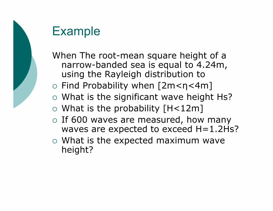
Example

When The root-mean square height of a narrow-banded sea is equal to 4.24m, using the Rayleigh distribution to

Find Probability when [2m<η<4m] What is the significant wave height Hs? What is the probability [H<12m] If 600 waves are measured, how many

waves are expected to exceed H=1.2Hs? What is the expected maximum wave

height?

7.3 Wave SpectraWave Spectra1. Discrete Spectra Wave Energy Density Spectra Wave amplitude spectra2. Continuous spectra Wave Energy Density Spectra** Wave Amplitude Spectra

See Figure 7.2 at pp194

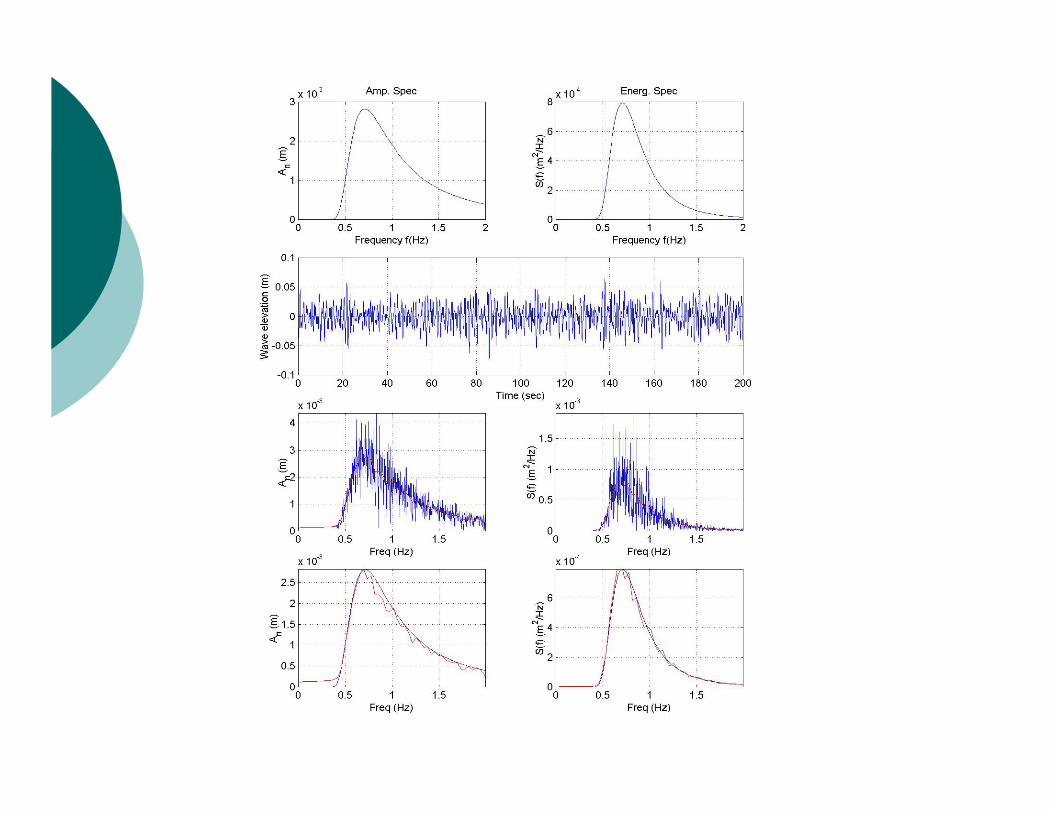
7.3.1 Spectral Analysis

1. How to obtain an energy density spectrum First deriving the discrete wave amplitude

spectrum (FFT) based on measured elevation Secondly deriving the discrete energy density

spectrum Then deriving the continuous energy density

spectrum In simulating an irregular wave train, the

above three steps are reversed. 2. How to simulate an irregular wave train

according to a given wave spectrum (later)

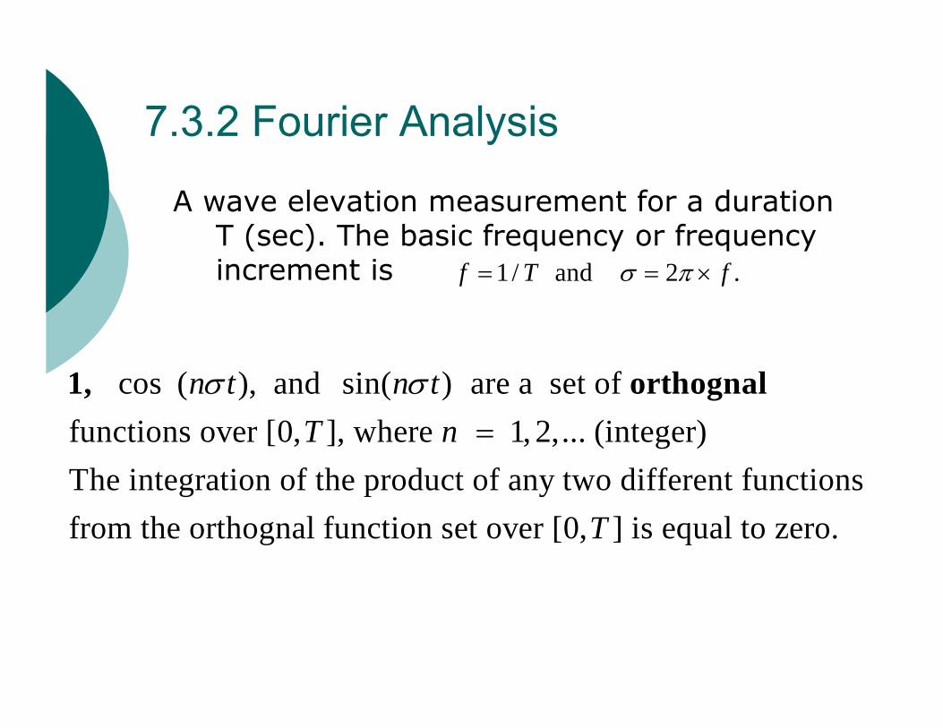
7.3.2 Fourier Analysis

A wave elevation measurement for a duration T (sec). The basic frequency or frequency increment is 1/ and 2 .f T f

cos ( ), and sin( ) are a set of functions over [0, ], where 1, 2,... (integer)The integration of the product of any two different functions from the orthognal function set ov

n t n tT n

1, orthognal

er [0, ] is equal to zero.T

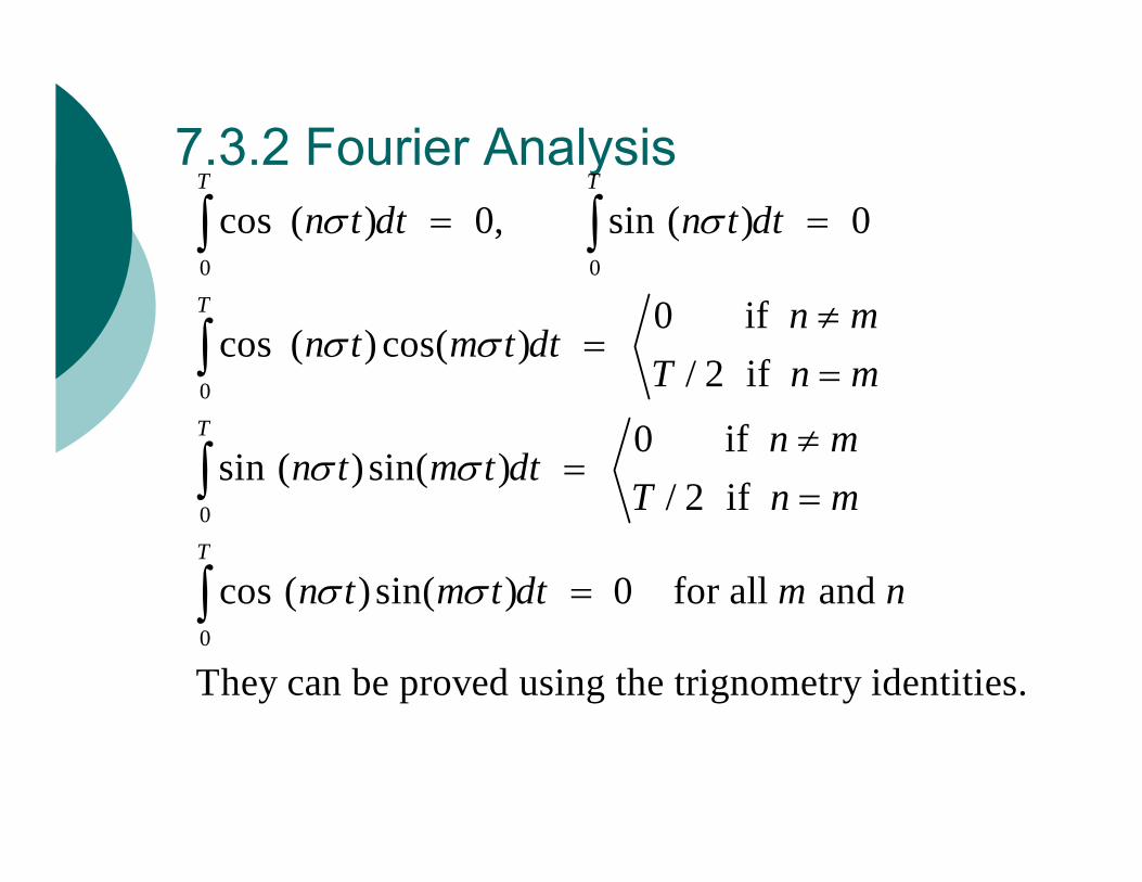
7.3.2 Fourier Analysis

0 0

0

0

0

cos ( ) 0, sin ( ) 0

0 if cos ( ) cos( )

/ 2 if

0 if sin ( ) sin( )

/ 2 if

cos ( ) sin( ) 0 for all and

They c

T T

T

T

T

n t dt n t dt

n mn t m t dt

T n m

n mn t m t dt

T n m

n t m t dt m n

an be proved using the trignometry identities.

7.3.2 Fourier Analysis (conti.)

01

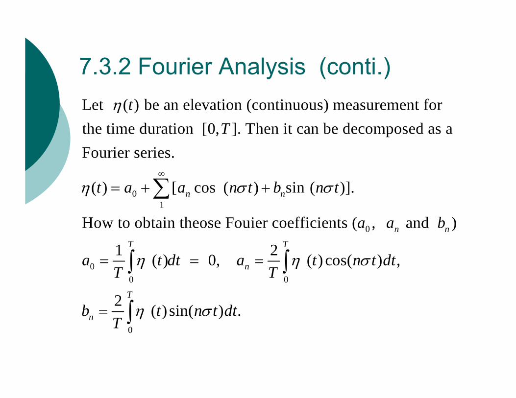
Let ( ) be an elevation (continuous) measurement for the time duration [0, ]. Then it can be decomposed as aFourier series.

( ) [ cos ( ) sin ( )].

How to obtain theose Fouier coefficie

n n

tT

t a a n t b n t

0

00 0

0

nts ( , and )

1 2 ( ) 0, ( ) cos( ) ,

2 ( ) sin( ) .

n n

T T

n

T

n

a a b

a t dt a t n t dtT T

b t n t dtT

7.3.2 Fourier Analysis (conti.)

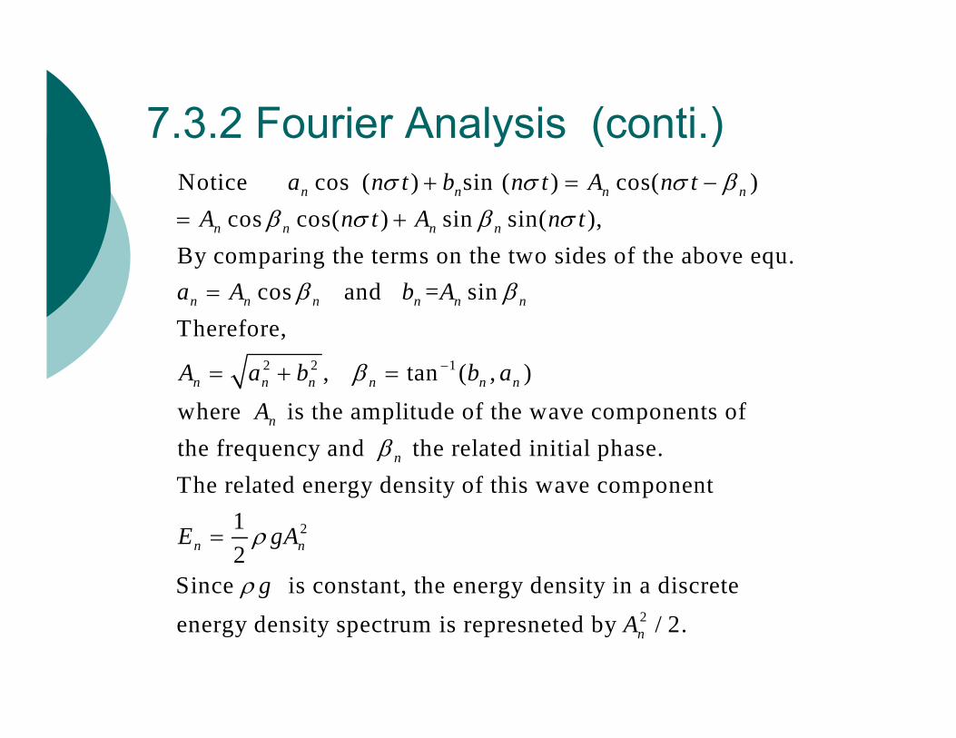
2 2 1

Notice cos ( ) sin ( ) cos( )cos cos( ) sin sin( ),

By comparing the terms on the two sides of the above equ.cos and = sin

Therefore,

, tan

n n n n

n n n n

n n n n n n

n n n n

a n t b n t A n tA n t A n t

a A b A

A a b

2

( , ) where is the amplitude of the wave components of the frequency and the related initial phase. The related energy density of this wave component

12

Since is constant, the en

n n

n

n

n n

b aA

E gA

g

2

ergy density in a discrete energy density spectrum is represneted by / 2.nA

To compute the Resultant wave properties

01

0

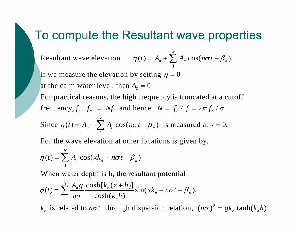
Resultant wave elevation ( ) cos( ).

If we measure the elevation by setting 0 at the calm water level, then 0.For practical reasons, the high frequency is truncated at a cutofff

n nt A A n t

A

01

1

requency, . and hence / 2 / .

Since ( ) cos( ) is measured at 0,

For the wave elevation at other locations is given by,

( ) cos( ).

When water depth

c c c c

n n

N

n n n

f f Nf N f f f

t A A n t x

t A xk n t

1

2

is h, the resultant potential cosh[ ( )]( ) sin( ).

cosh( )

is related to through dispersion relation, ( ) tanh( )

Nn n

n nn

n n n

A g k z ht xk n tn k h

k n t n gk k h

Resultant wave properties

1

1

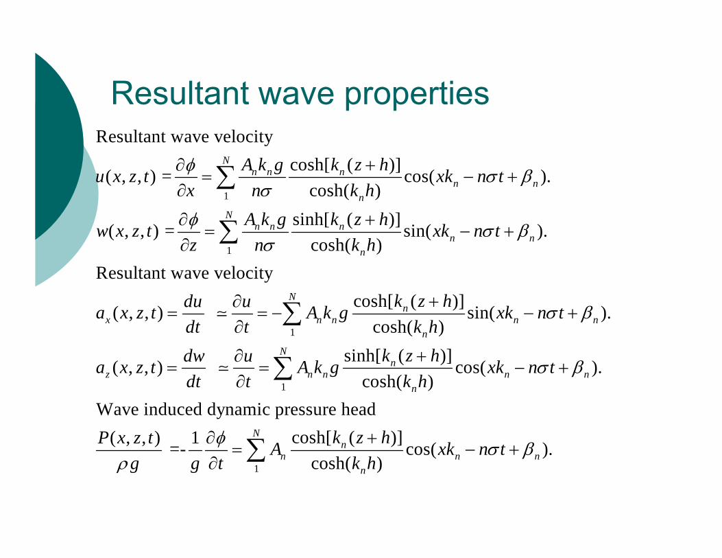
Resultant wave velocity cosh[ ( )]( , , ) = cos( ).

cosh( )sinh[ ( )]( , , ) = sin( ).

cosh( )Resultant wave velocity

( , , )

Nn n n

n nn

Nn n n

n nn

x

A k g k z hu x z t xk n tx n k h

A k g k z hw x z t xk n tz n k h

du ua x z tdt t

1

1

cosh[ ( )] sin( ).cosh( )

sinh[ ( )]( , , ) cos( ).cosh( )

Wave induced dynamic pressure headcosh[ ( )]( , , ) 1 =- cos(

cosh( )

Nn

n n n nn

Nn

z n n n nn

nn n

n

k z hA k g xk n tk h

k z hdw ua x z t A k g xk n tdt t k h

k z hP x z t A xkg g t k h

1).

N

nn t

Parseval’s Theorem

2

0

2

0

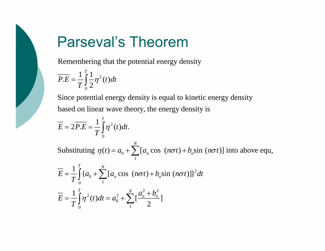
Remembering that the potential energy density

1 1. ( )2

Since potential energy density is equal to kinetic energy densitybased on linear wave theory, the energy density is

12 . ( ) .

S

T

T

P E t dtT

E P E t dtT

01

20

10

2 22 2

010

ubstituting ( ) [ cos ( ) sin ( )] into above equ,

1 { [ cos ( ) sin ( )]}

1 ( ) [ ] 2

N

n n

T N

n n

T Nn n

t a a n t b n t

E a a n t b n t dtT

a bE t dt aT

Continuous wave spectra

There are many theoretical spectrum to present ocean waves. The most common ones are:

1. JONSWAP spectrum (North sea)

2. Pierson-Moskowitz Spectrum

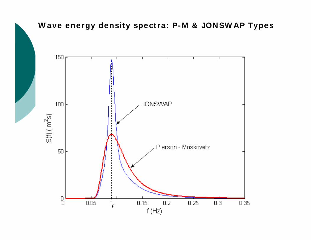
Wave energy density spectra: P-M & JONSWAP Types

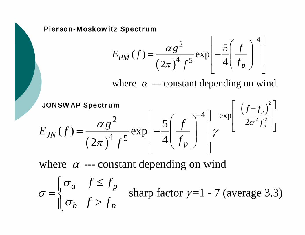
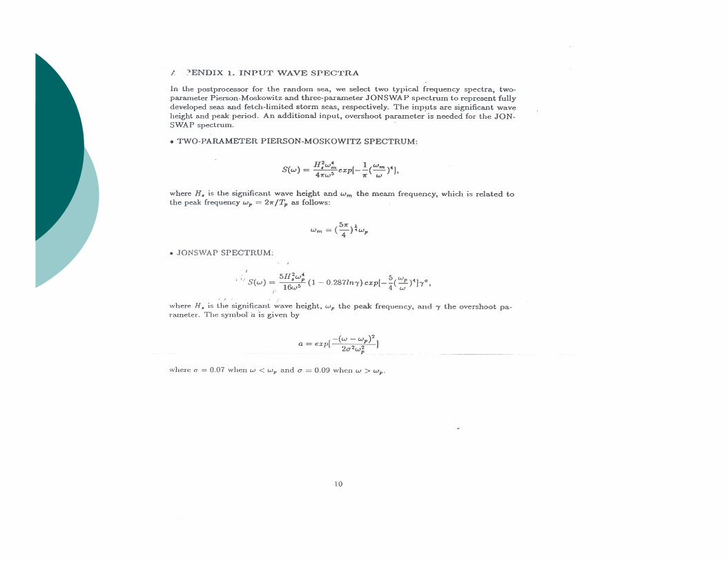
Pierson-Moskowitz Spectrum

42

4 55( ) exp42

where --- constant depending on wind

PMp

g fE fff

JONSWAP Spectrum

2

2 24 exp2 2

4 5

5( ) exp42

where --- constant depending on wind

sharp factor =1 - 7 (average 3.3)

p

p

f ff

JNp

a p

b p

g fE fff

f f

f f

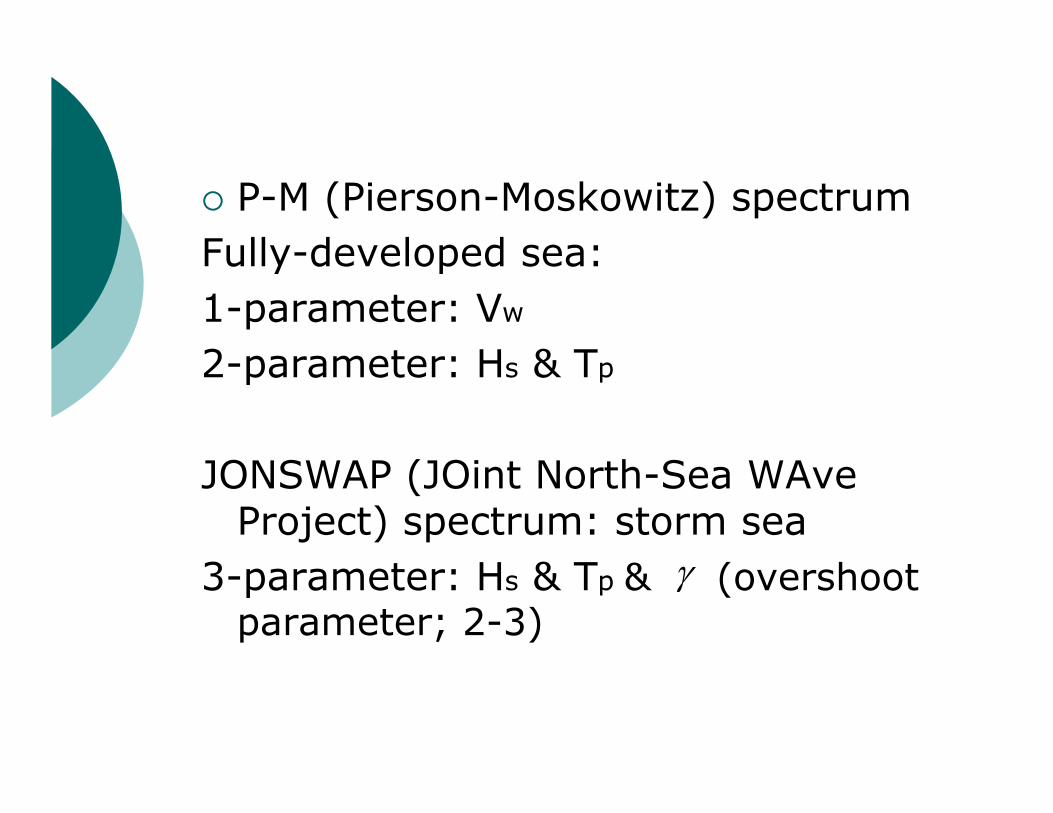
P-M (Pierson-Moskowitz) spectrumFully-developed sea:1-parameter: Vw

2-parameter: Hs & Tp

JONSWAP (JOint North-Sea WAve Project) spectrum: storm sea

3-parameter: Hs & Tp & (overshoot parameter; 2-3)

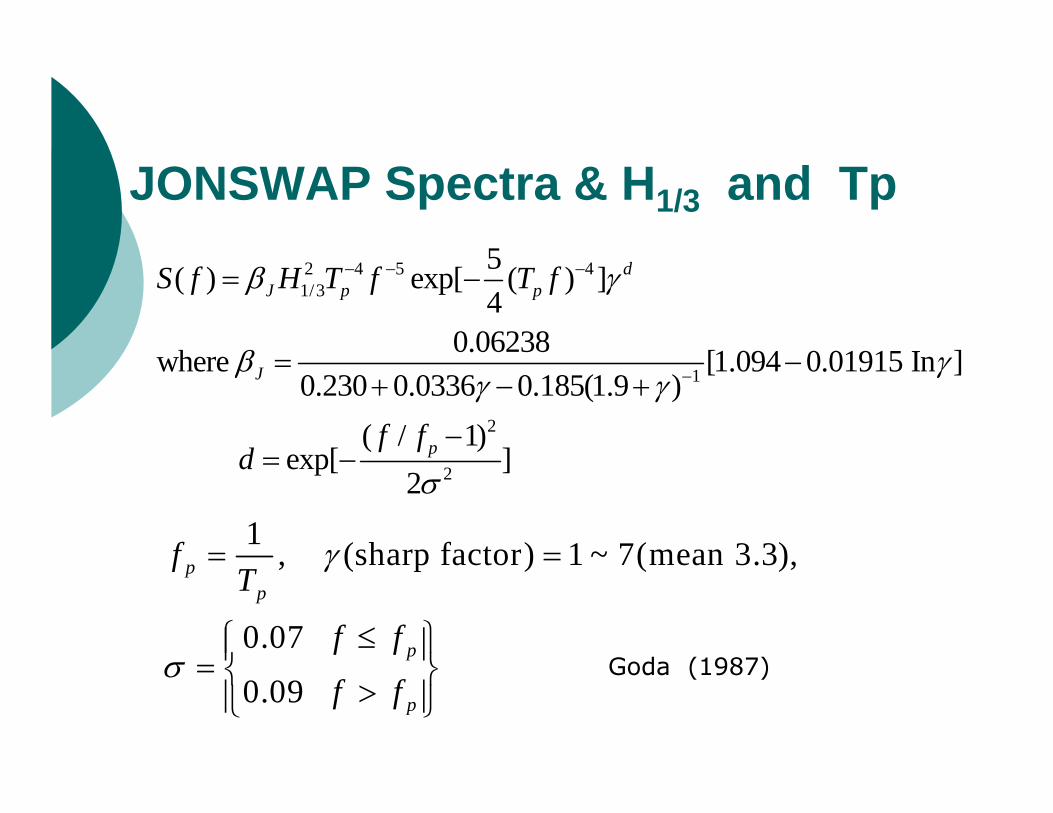
JONSWAP Spectra & H1/3 and Tp2 4 5 41/3

1

2

2

5( ) exp[ ( ) ]4

0.06238where [1.094 0.01915 In ]0.230 0.0336 0.185(1.9 )

( / 1) exp[ ]

2

dJ p p

J

p

S f H T f T f

f fd

1 , (sharp factor) 1 ~ 7(mean 3.3),

0.07

0.09

pp

p

p

fT

f f

f f

Goda (1987)

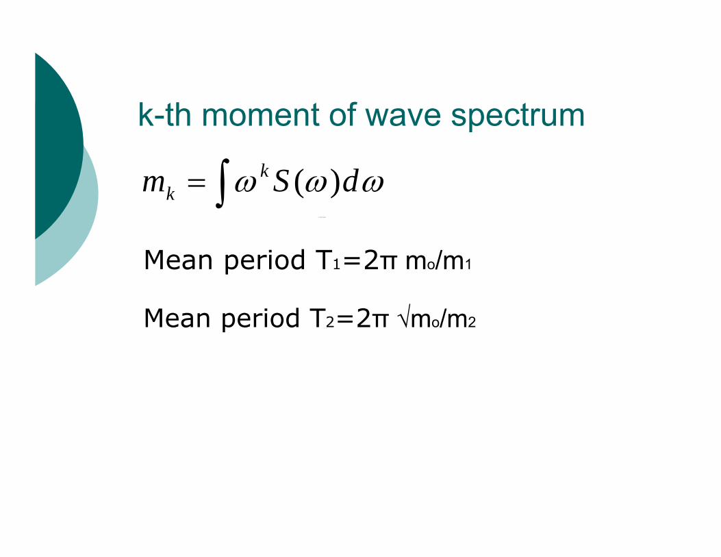
k-th moment of wave spectrum

Mean period T1=2π mo/m1

Mean period T2=2π √mo/m2

( )kkm S d

( )kkm S d

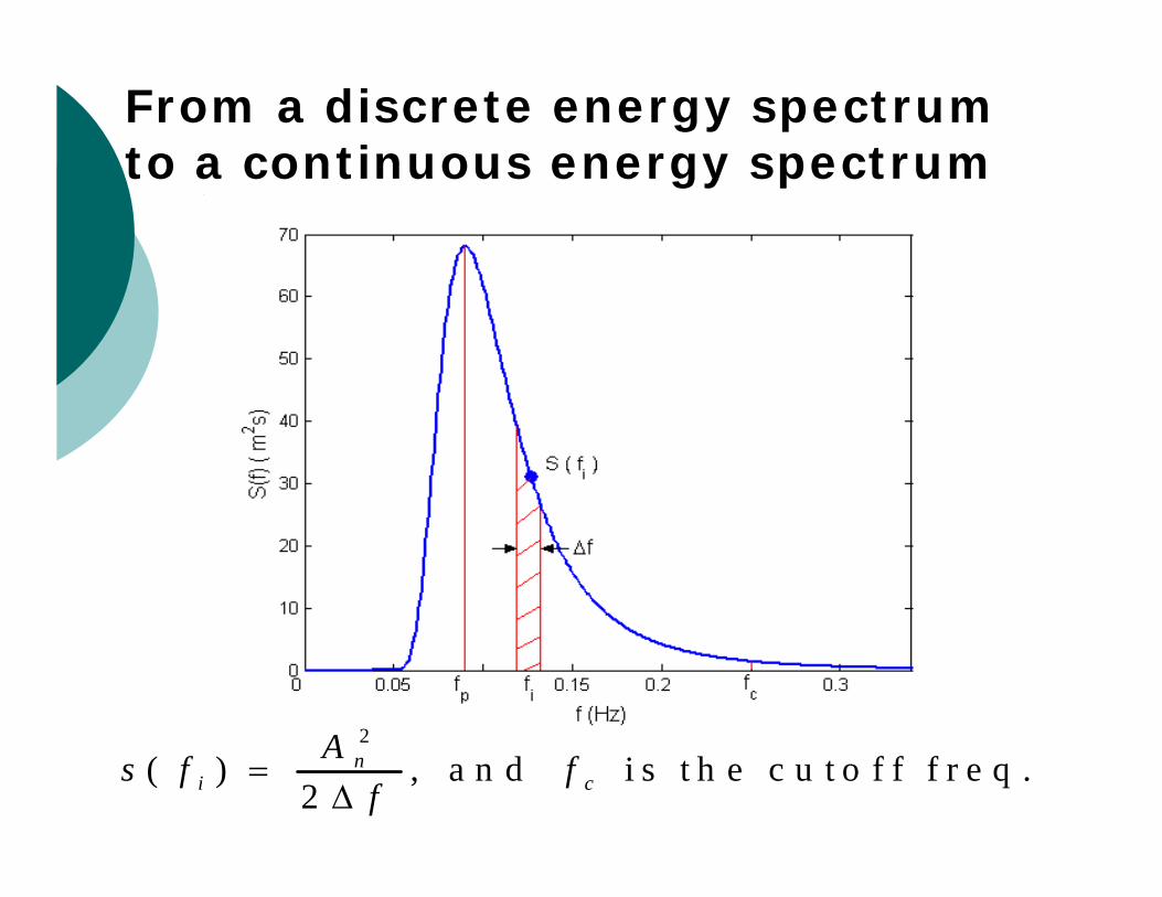
From a discrete energy spectrum to a continuous energy spectrum

2

( ) , a n d i s t h e c u t o f f f r e q .2

ni c

As f ff

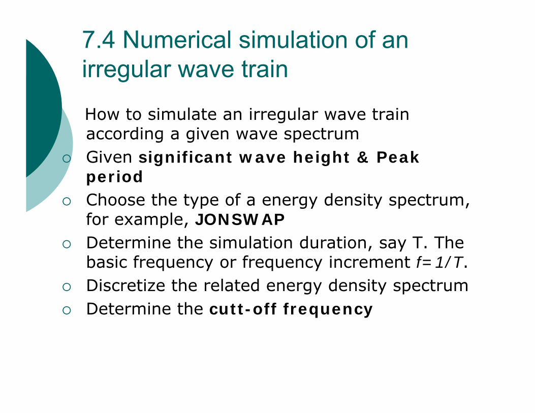
7.4 Numerical simulation of an irregular wave train

How to simulate an irregular wave train according a given wave spectrum

Given significant wave height & Peak period

Choose the type of a energy density spectrum, for example, JONSWAP

Determine the simulation duration, say T. The basic frequency or frequency increment f=1/T.

Discretize the related energy density spectrum Determine the cutt-off frequency

7.4 Numerical simulation (conti.)At each discrete frequency nf, the amplitude of nth wave components is given by

The initial phase of each wave component is randomly selected between –pi and pi.

The resultant wave elevation is hence given by

2* ( )* ,where and 1/ is the frequency increment.

n i

i

A S f ff nf f T

1

1

( ) cos( ).

W hen water depth is h, the resultant potential cosh[ ( )]( ) sin( ).

cosh( )

N

n n n

Nn n

n nn

t A xk n t

A g k z ht xk n tn k h

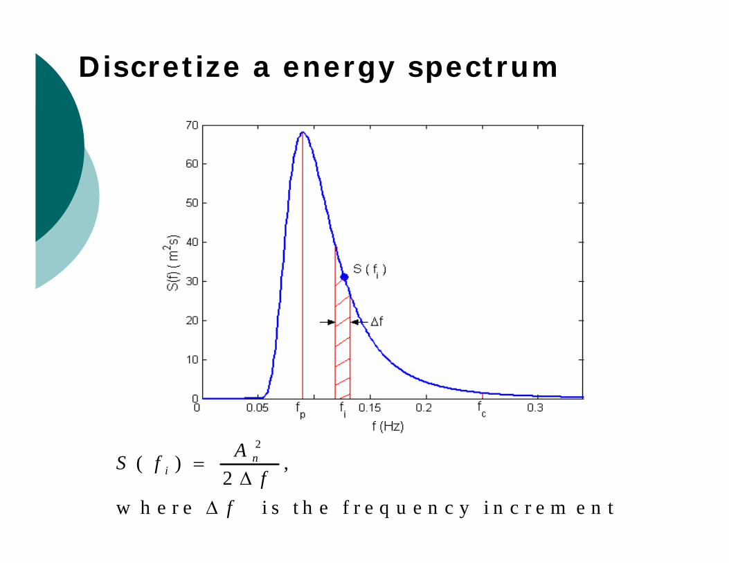
Discretize a energy spectrum

2

( ) , 2

w h e r e i s t h e f r e q u e n c y i n c r e m e n t

ni

AS ff

f

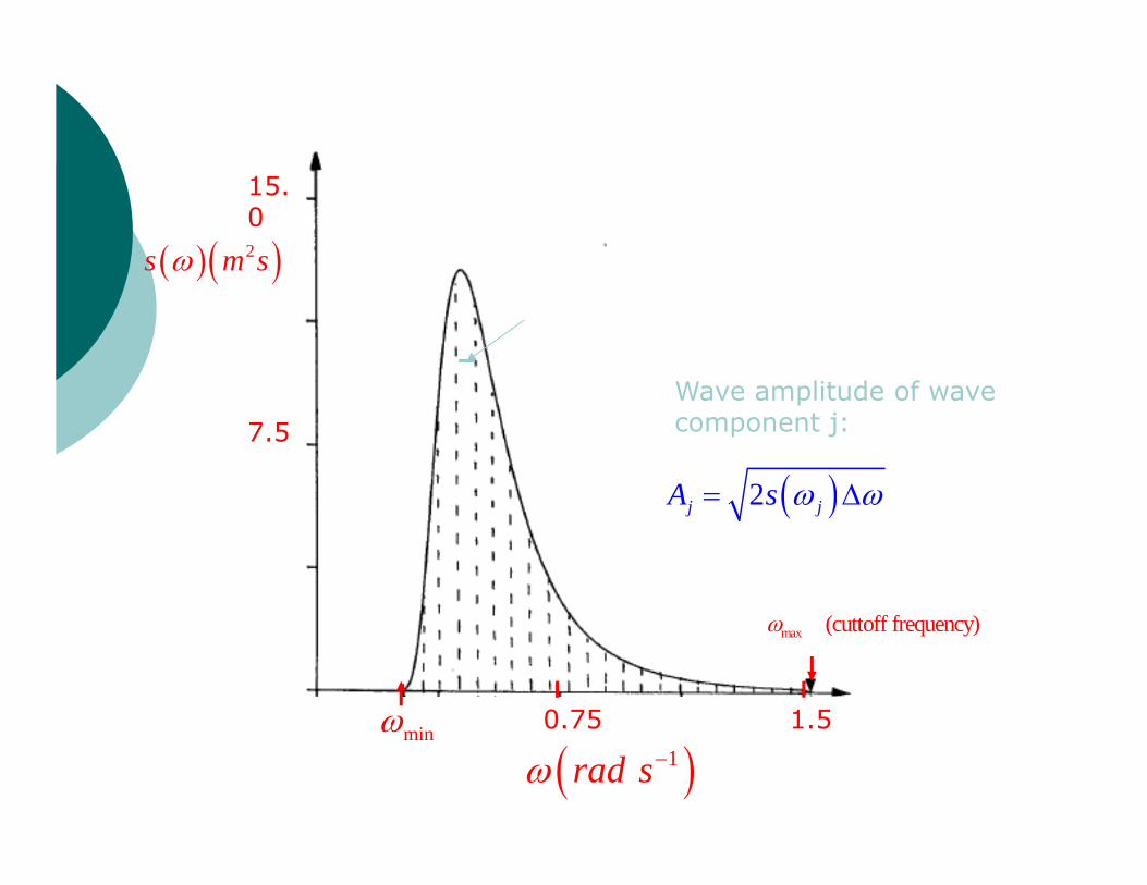
2s m s

15.0

7.5

0.75 1.5min

max (cuttoff frequency)

1rad s

Wave amplitude of wavecomponent j:

2j jA s

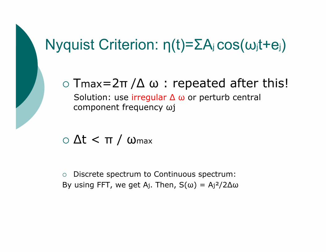
Nyquist Criterion: η(t)=ΣAj cos(ωjt+ej)

Tmax=2π /∆ ω : repeated after this!Solution: use irregular ∆ ω or perturb central component frequency ωj

∆t < π / ωmax

Discrete spectrum to Continuous spectrum:By using FFT, we get Aj. Then, S(ω) = Aj²/2∆ω

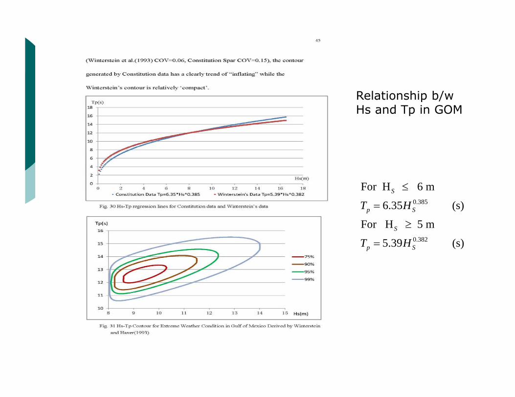
Relationship b/wHs and Tp in GOM

0.385

0.382

For H 6 m

6.35 (s)

For H 5 m

5.39 (s)

S

p S

S

p S

T H

T H

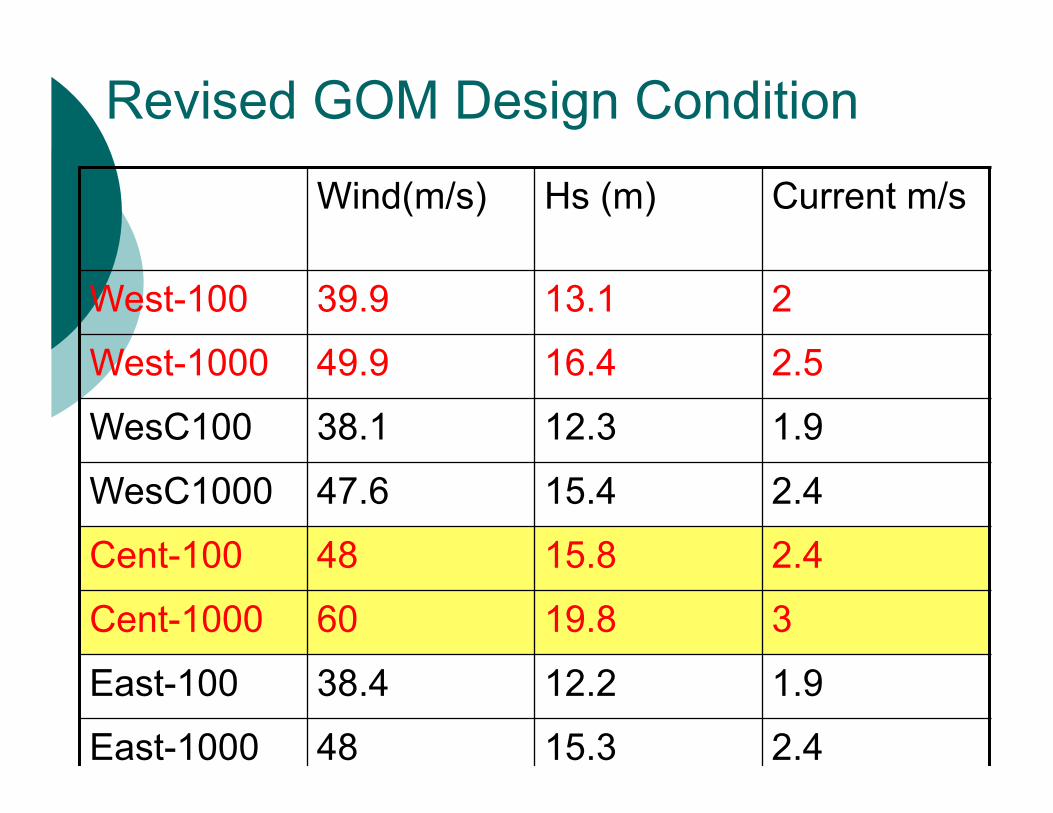
Revised GOM Design Condition

Wind(m/s) Hs (m) Current m/s

West-100 39.9 13.1 2

West-1000 49.9 16.4 2.5

WesC100 38.1 12.3 1.9

WesC1000 47.6 15.4 2.4

Cent-100 48 15.8 2.4

Cent-1000 60 19.8 3

East-100 38.4 12.2 1.9

East-1000 48 15.3 2.4

Return Period & the Probability of the Occurrence of the Storm in A Given Year

( )kkm S d

The Return period of a storm, such as 100-year period , 50-year period, etc, indicates the probability of the storm (with the related strength) occurring during any given year.

For example, 100-year return period means the probability of the occurrence of the related storm is equal to 0.01 in any given year. Similarly, 50-year return period is related the probability of 0.02.

The probability of occurrence in a given year = 1/(return period).

Return Period & the Probability of the Occurrence of the Storm in the Life Span of A Platform

( )kkm S d

Assuming that the service life of a floating structure is 25 years, what is the probability of 100-year storm occurring at least once during its service life?

The probability depends on the length of service life and the return period.

How to compute it?

Return Period & the Probability of the Occurrence of the Storm in the Life Span of A Platform

( )kkm S d

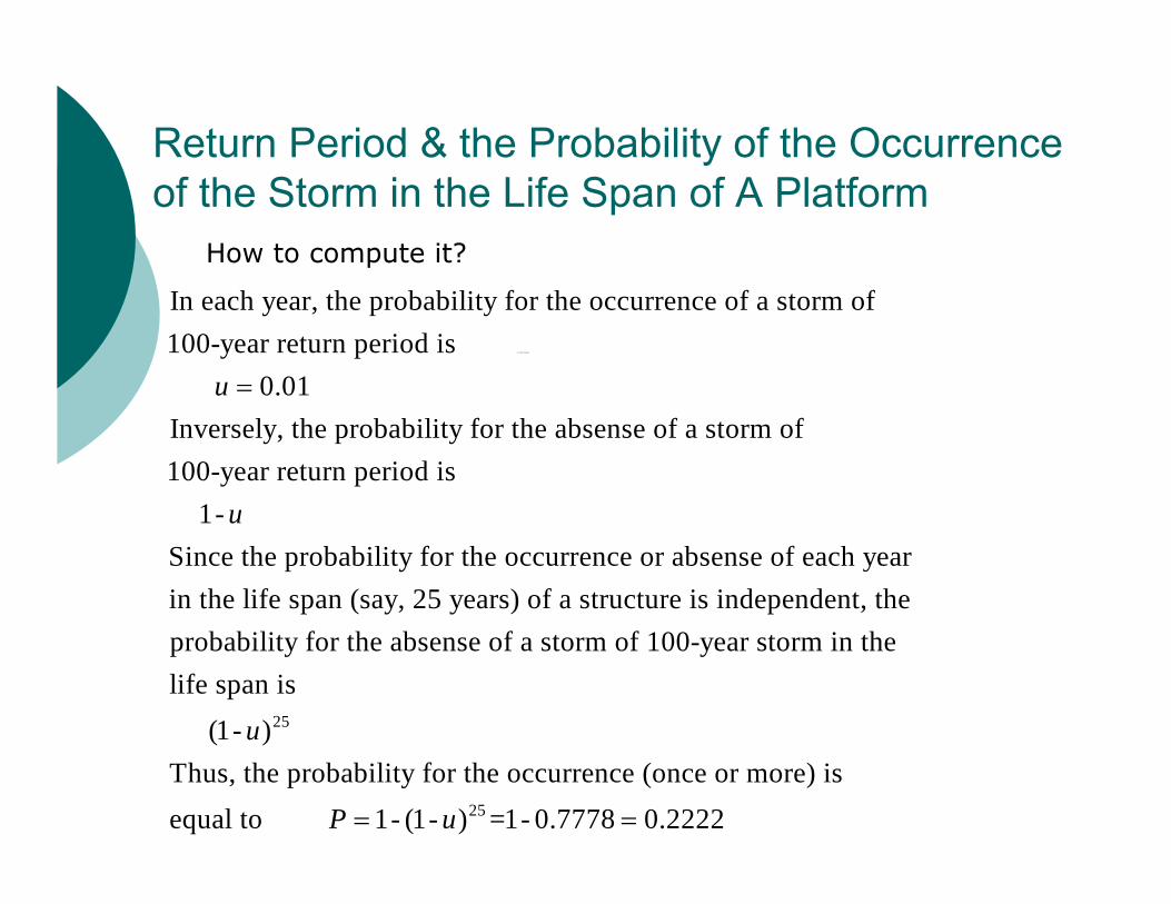
How to compute it?

In each year, the probability for the occurrence of a storm of100-year return period is 0.01Inversely, the probability for the absense of a storm of100-year return period is 1-Since the pro

u

u

bability for the occurrence or absense of each year in the life span (say, 25 years) of a structure is independent, the probability for the absense of a storm of 100-year storm in thelife span is 25

25

(1- ) Thus, the probability for the occurrence (once or more) isequal to 1- (1- ) =1- 0.7778 0.2222

u

P u

Return Period & the Probability of the Occurrence of the Storm in the Life Span of A Platform

( )kkm S d

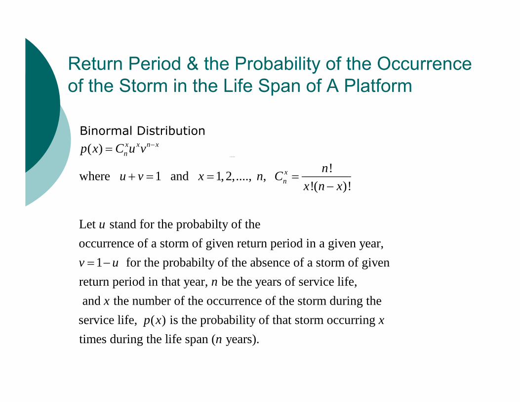
Binormal Distribution( )

!where 1 and 1, 2,...., , !( )!

Let stand for the probabilty of theoccurrence of a storm of given return period in a given year,

1 for the probabilty of the abs

x x n xn

xn

p x C u vnu v x n C

x n x

u

v u

ence of a storm of given return period in that year, be the years of service life, and the number of the occurrence of the storm during theservice life, ( ) is the probability of that storm occu

nx

p x rring times during the life span ( years).

xn

Return Period & the Probability of the Occurrence of the Storm in the Life Span of A Platform

( )kkm S d

25 2-

251 1

( )

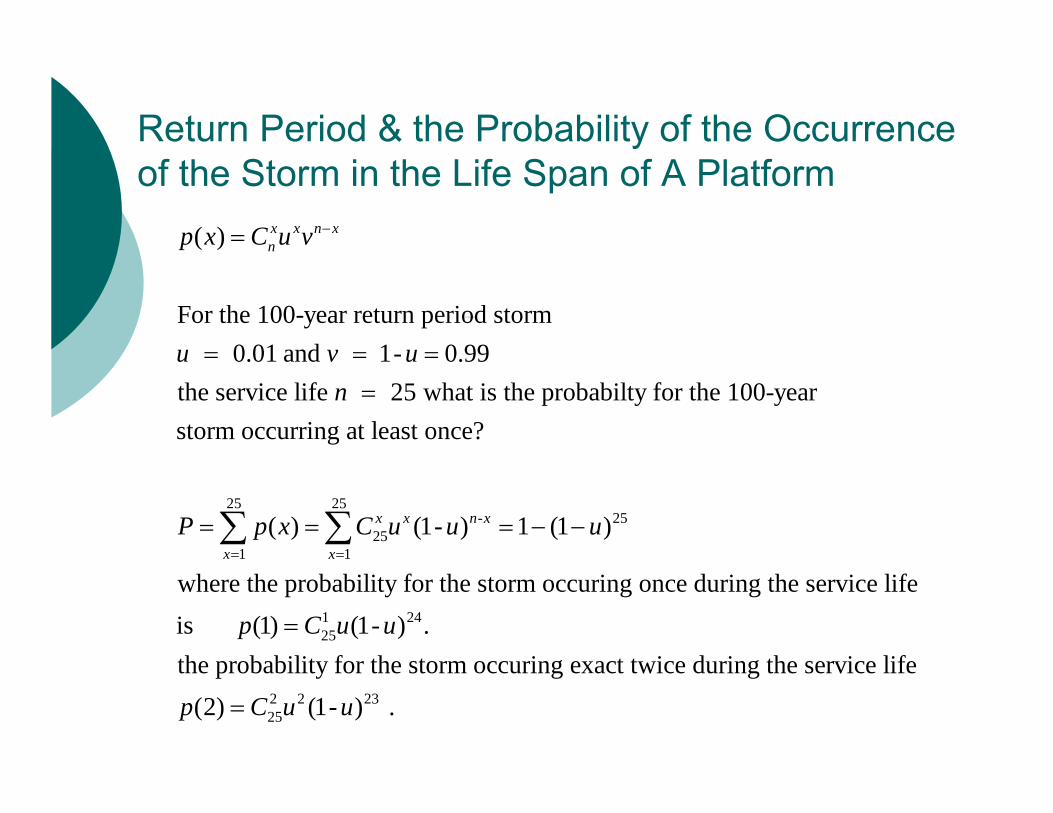
For the 100-year return period storm 0.01 and 1- 0.99

the service life 25 what is the probabilty for the 100-yearstorm occurring at least once?

( ) (1- )

x x n xn

x x n x

x x

p x C u v

u v un

P p x C u u

5

25

1 2425

2 225

1 (1 )

where the probability for the storm occuring once during the service life is (1) (1- ) .the probability for the storm occuring exact twice during the service life

(2) (1

u

p C u u

p C u

23- ) .u