Chapter Two

2-1McGraw-Hill/Irwin ©2007, The McGraw-Hill Companies, All Rights Reserved

Chapter TwoDeterminants of

Interest Rates


Interest Rate Fundamentals

• Nominal interest rates - the interest rate actually observed in financial markets– directly affect the value (price) of most

securities traded in the market

– affect the relationship between spot and forward FX rates

• Nominal interest rates - the interest rate actually observed in financial markets– directly affect the value (price) of most

securities traded in the market

– affect the relationship between spot and forward FX rates


Time Value of Money and Interest Rates

• Assumes the basic notion that a dollar received today is worth more than a dollar received at some future date

• Compound interest– interest earned on an investment is reinvested

• Simple interest– interest earned on an investment is not

reinvested

• Assumes the basic notion that a dollar received today is worth more than a dollar received at some future date

• Compound interest– interest earned on an investment is reinvested

• Simple interest– interest earned on an investment is not

reinvested


Calculation of Simple Interest

Value = Principal + Interest (year 1) + Interest (year 2)

Example: $1,000 to invest for a period of two years at 12 percent

Value = $1,000 + $1,000(.12) + $1,000(.12)

= $1,000 + $1,000(.12)(2)

= $1,240

Value = Principal + Interest (year 1) + Interest (year 2)

Example: $1,000 to invest for a period of two years at 12 percent

Value = $1,000 + $1,000(.12) + $1,000(.12)

= $1,000 + $1,000(.12)(2)

= $1,240


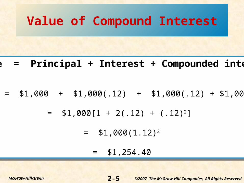
Value of Compound Interest

Value = Principal + Interest + Compounded interest

Value = $1,000 + $1,000(.12) + $1,000(.12) + $1,000(.12)

= $1,000[1 + 2(.12) + (.12)2]

= $1,000(1.12)2

= $1,254.40

Value = Principal + Interest + Compounded interest

Value = $1,000 + $1,000(.12) + $1,000(.12) + $1,000(.12)

= $1,000[1 + 2(.12) + (.12)2]

= $1,000(1.12)2

= $1,254.40


Present Value of a Lump Sum

• PV function converts cash flows received over a future investment horizon into an equivalent (present) value by discounting future cash flows back to present using current market interest rate

– lump sum payment

– annuity

• PVs decrease as interest rates increase

• PV function converts cash flows received over a future investment horizon into an equivalent (present) value by discounting future cash flows back to present using current market interest rate

– lump sum payment

– annuity

• PVs decrease as interest rates increase


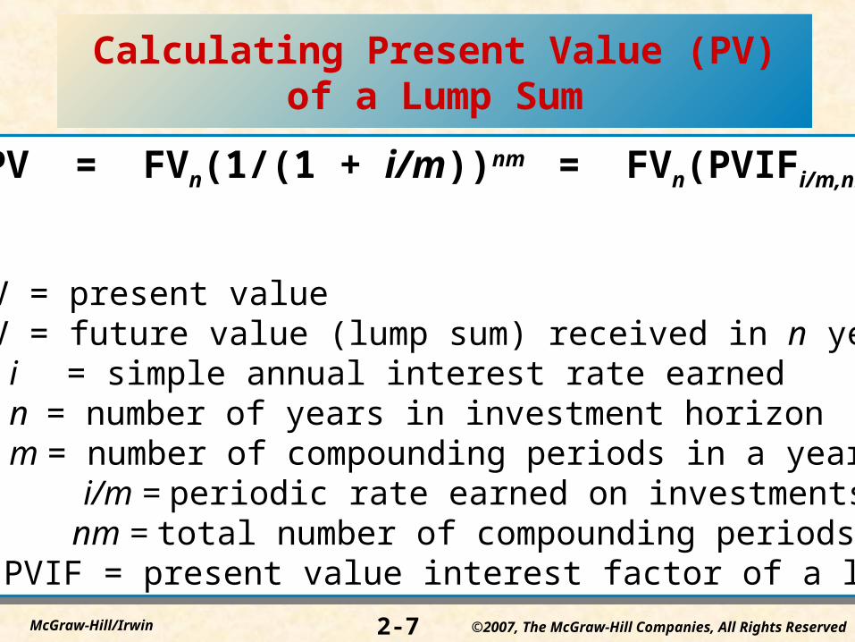
Calculating Present Value (PV) of a Lump Sum

PV = FVn(1/(1 + i/m))nm = FVn(PVIFi/m,nm)

where:PV = present valueFV = future value (lump sum) received in n years i = simple annual interest rate earned n = number of years in investment horizon m = number of compounding periods in a year

i/m = periodic rate earned on investments nm = total number of compounding periods PVIF = present value interest factor of a lump sum

PV = FVn(1/(1 + i/m))nm = FVn(PVIFi/m,nm)

where:PV = present valueFV = future value (lump sum) received in n years i = simple annual interest rate earned n = number of years in investment horizon m = number of compounding periods in a year

i/m = periodic rate earned on investments nm = total number of compounding periods PVIF = present value interest factor of a lump sum


Calculating Present Value of a Lump Sum

• You are offered a security investment that pays $10,000 at the end of 6 years in exchange for a fixed payment today.

• PV = FV(PVIFi/m,nm)

• at 8% interest - = $10,000(0.630170) = $6,301.70

• at 12% interest - = $10,000(0.506631) = $5,066.31

• at 16% interest - = $10,000(0.410442) = $4,104.42

• You are offered a security investment that pays $10,000 at the end of 6 years in exchange for a fixed payment today.

• PV = FV(PVIFi/m,nm)

• at 8% interest - = $10,000(0.630170) = $6,301.70

• at 12% interest - = $10,000(0.506631) = $5,066.31

• at 16% interest - = $10,000(0.410442) = $4,104.42


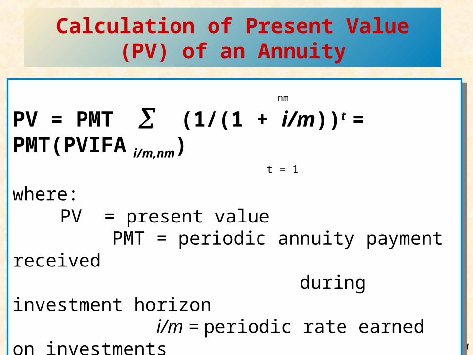
Calculation of Present Value (PV) of an Annuity

nm

PV = PMT (1/(1 + i/m))t = PMT(PVIFA i/m,nm)

t = 1

where:PV = present value

PMT = periodic annuity payment received during investment horizon i/m = periodic rate earned on investments nm = total number of compounding periods PVIFA = present value interest factor of an annuity

nm

PV = PMT (1/(1 + i/m))t = PMT(PVIFA i/m,nm)

t = 1

where:PV = present value

PMT = periodic annuity payment received during investment horizon i/m = periodic rate earned on investments nm = total number of compounding periods PVIFA = present value interest factor of an annuity


Calculation of Present Value of an Annuity

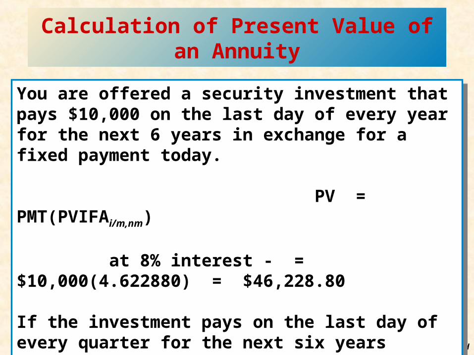
You are offered a security investment that pays $10,000 on the last day of every year for the next 6 years in exchange for a fixed payment today.

PV = PMT(PVIFAi/m,nm)

at 8% interest - = $10,000(4.622880) = $46,228.80

If the investment pays on the last day of every quarter for the next six years

at 8% interest - = $10,000(18.913926) = $189,139.26

You are offered a security investment that pays $10,000 on the last day of every year for the next 6 years in exchange for a fixed payment today.

PV = PMT(PVIFAi/m,nm)

at 8% interest - = $10,000(4.622880) = $46,228.80

If the investment pays on the last day of every quarter for the next six years

at 8% interest - = $10,000(18.913926) = $189,139.26


Future Values

• Translate cash flows received during an investment period to a terminal (future) value at the end of an investment horizon

• FV increases with both the time horizon and the interest rate

• Translate cash flows received during an investment period to a terminal (future) value at the end of an investment horizon

• FV increases with both the time horizon and the interest rate


Future Values Equations

FV of lump sum equation

FVn = PV(1 + i/m)nm = PV(FVIF i/m, nm)

FV of annuity payment equation

(nm-1)

FVn = PMT (1 + i/m)t = PMT(FVIFAi/m, mn) (t = 0)

FV of lump sum equation

FVn = PV(1 + i/m)nm = PV(FVIF i/m, nm)

FV of annuity payment equation

(nm-1)

FVn = PMT (1 + i/m)t = PMT(FVIFAi/m, mn) (t = 0)


Calculation of Future Value of a Lump Sum

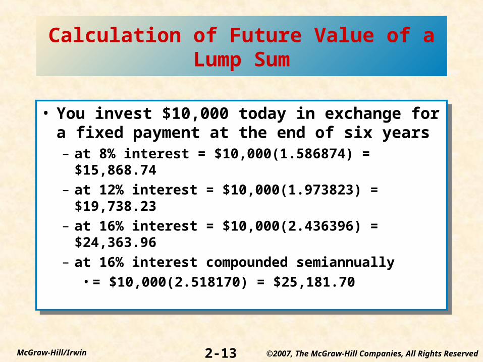
• You invest $10,000 today in exchange for a fixed payment at the end of six years– at 8% interest = $10,000(1.586874) = $15,868.74

– at 12% interest = $10,000(1.973823) = $19,738.23

– at 16% interest = $10,000(2.436396) = $24,363.96

– at 16% interest compounded semiannually

• = $10,000(2.518170) = $25,181.70

• You invest $10,000 today in exchange for a fixed payment at the end of six years– at 8% interest = $10,000(1.586874) = $15,868.74

– at 12% interest = $10,000(1.973823) = $19,738.23

– at 16% interest = $10,000(2.436396) = $24,363.96

– at 16% interest compounded semiannually

• = $10,000(2.518170) = $25,181.70


Calculation of the Future Value of an Annuity

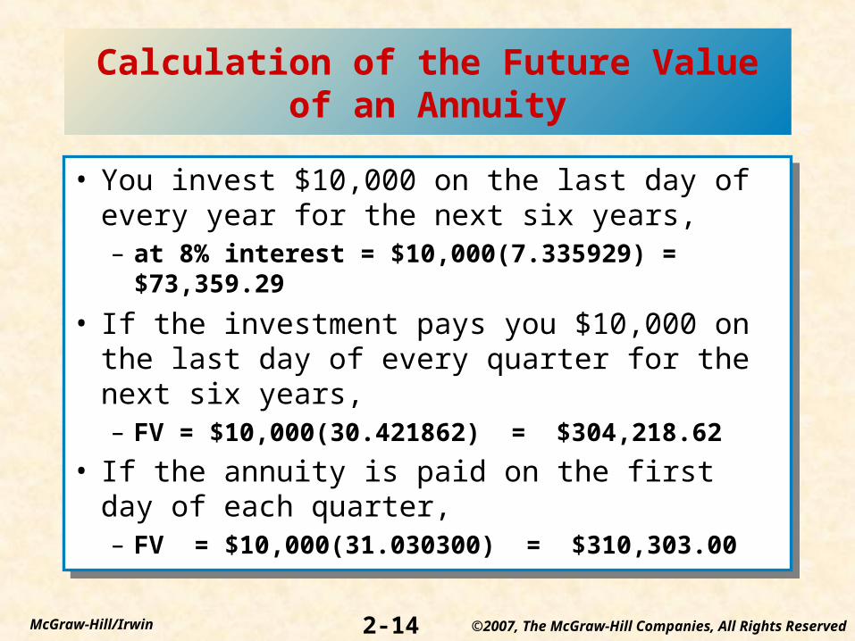
• You invest $10,000 on the last day of every year for the next six years,– at 8% interest = $10,000(7.335929) = $73,359.29

• If the investment pays you $10,000 on the last day of every quarter for the next six years,– FV = $10,000(30.421862) = $304,218.62

• If the annuity is paid on the first day of each quarter, – FV = $10,000(31.030300) = $310,303.00

• You invest $10,000 on the last day of every year for the next six years,– at 8% interest = $10,000(7.335929) = $73,359.29

• If the investment pays you $10,000 on the last day of every quarter for the next six years,– FV = $10,000(30.421862) = $304,218.62

• If the annuity is paid on the first day of each quarter, – FV = $10,000(31.030300) = $310,303.00


Relation between Interest Rates and Present and Future Values

Present Value(PV)

Interest Rate

FutureValue(FV)

Interest Rate


Effective or Equivalent Annual Return (EAR)

Rate earned over a 12 – month period taking the compounding of interest into account.

EAR = (1 + r) c – 1

Where c = number of compounding periods per year

Rate earned over a 12 – month period taking the compounding of interest into account.

EAR = (1 + r) c – 1

Where c = number of compounding periods per year


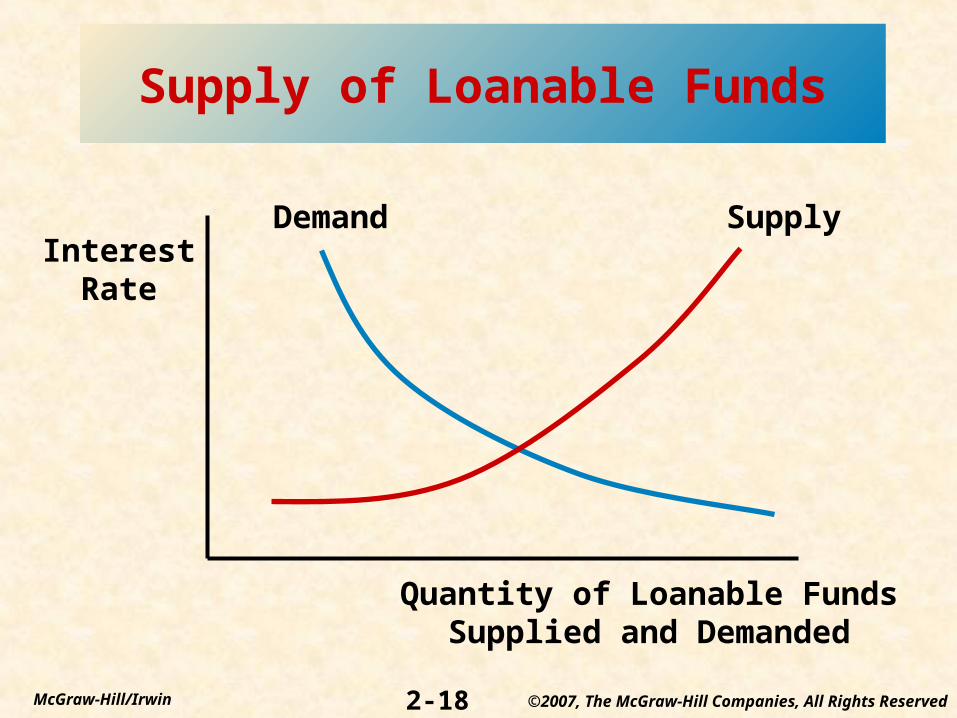
Loanable Funds Theory

• A theory of interest rate determination that views equilibrium interest rates in financial markets as a result of the supply and demand for loanable funds

• A theory of interest rate determination that views equilibrium interest rates in financial markets as a result of the supply and demand for loanable funds


Supply of Loanable Funds

InterestRate

Quantity of Loanable FundsSupplied and Demanded

Demand Supply


Funds Supplied and Demanded by Various Groups (in billions of dollars)

Funds Supplied Funds Demanded Net

Households $34,860.7 $15,197.4 $19,663.3Business - nonfinancial 12,679.2 30,779.2 -12,100.0Business - financial 31,547.9 45061.3 -13,513.4Government units 12,574.5 6,695.2 5,879.3Foreign participants 8,426.7 2,355.9 6,070.8

Funds Supplied Funds Demanded Net

Households $34,860.7 $15,197.4 $19,663.3Business - nonfinancial 12,679.2 30,779.2 -12,100.0Business - financial 31,547.9 45061.3 -13,513.4Government units 12,574.5 6,695.2 5,879.3Foreign participants 8,426.7 2,355.9 6,070.8


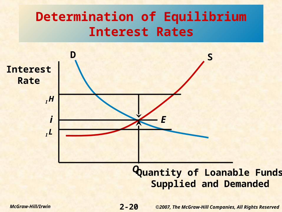
Determination of Equilibrium Interest Rates

InterestRate

Quantity of Loanable FundsSupplied and Demanded

D S

I H

i

I L

E

Q


Effect on Interest rates from a Shift in the Demand Curve for or Supply curve of

Loanable FundsIncreased supply of loanable funds

Quantity ofFunds Supplied

InterestRate DD SS

SS*

EE*

Q*

i*

Q**

i**

Increased demand for loanable funds

Quantity of Funds Demanded

DDDD* SS

EE*

i*

i**

Q* Q**


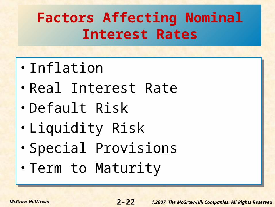
Factors Affecting Nominal Interest Rates

• Inflation

• Real Interest Rate

• Default Risk

• Liquidity Risk

• Special Provisions

• Term to Maturity

• Inflation

• Real Interest Rate

• Default Risk

• Liquidity Risk

• Special Provisions

• Term to Maturity


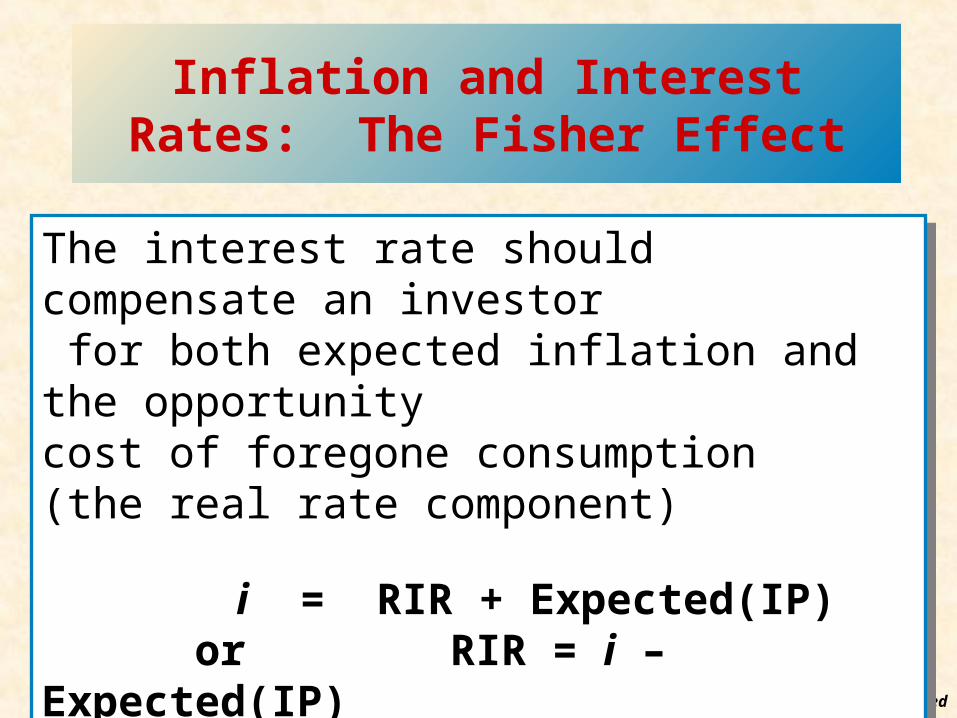
Inflation and Interest Rates: The Fisher Effect

The interest rate should compensate an investor for both expected inflation and the opportunity cost of foregone consumption (the real rate component)

i = RIR + Expected(IP) or RIR = i – Expected(IP)

Example: 3.49% - 1.60% = 1.89%

The interest rate should compensate an investor for both expected inflation and the opportunity cost of foregone consumption (the real rate component)

i = RIR + Expected(IP) or RIR = i – Expected(IP)

Example: 3.49% - 1.60% = 1.89%


Default Risk and Interest Rates

The risk that a security’s issuer will default on that security by being late on or missing an interest or principal payment

DRPj = ijt - iTt

Example for December 2003: DRPAaa = 5.66% - 4.01% = 1.65%DRPBaa = 6.76% - 4.01% = 2.75%

The risk that a security’s issuer will default on that security by being late on or missing an interest or principal payment

DRPj = ijt - iTt

Example for December 2003: DRPAaa = 5.66% - 4.01% = 1.65%DRPBaa = 6.76% - 4.01% = 2.75%


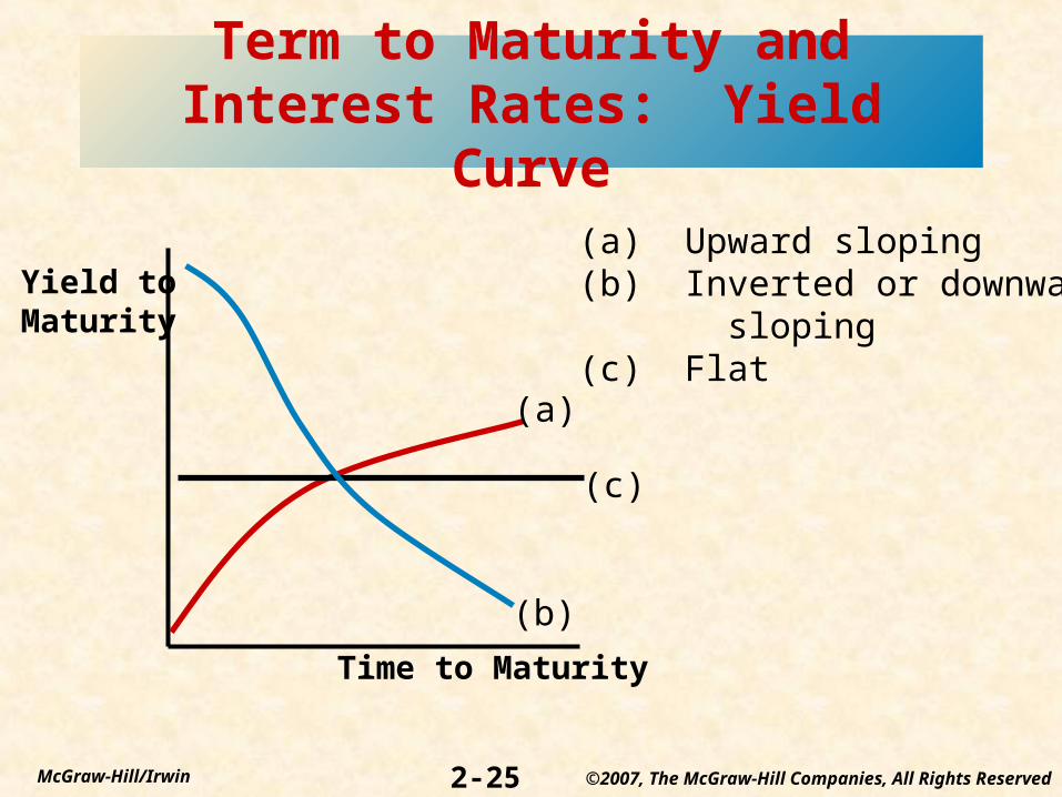
Term to Maturity and Interest Rates: Yield Curve

Yield toMaturity

Time to Maturity

(a)

(b)

(c)

(a) Upward sloping(b) Inverted or downward sloping(c) Flat


Term Structure of Interest Rates

• Unbiased Expectations Theory

• Liquidity Premium Theory

• Market Segmentation Theory

• Unbiased Expectations Theory

• Liquidity Premium Theory

• Market Segmentation Theory


Forecasting Interest Rates

Forward rate is an expected or “implied” rate on a security that is to be originated at some point in the future using the unbiased expectations theory _ _ 1R2 = [(1 + 1R1)(1 + (2f1))]1/2 - 1

where 2 f1 = expected one-year rate for year 2, or the implied forward one-year rate for next year

Forward rate is an expected or “implied” rate on a security that is to be originated at some point in the future using the unbiased expectations theory _ _ 1R2 = [(1 + 1R1)(1 + (2f1))]1/2 - 1

where 2 f1 = expected one-year rate for year 2, or the implied forward one-year rate for next year

Documents

Chapter Two