26

CHAPTER THREE: LEVELS AND TRENDS IN HUMAN DEVELOPMENT IN INDIA AND STATES

3.1.Introduction:

The UNDP has developed a set of composite indices such as human development index (HDI),

Human Poverty Index (HPI) and Gender related Development Index (GDI) for measuring the level

of development and disparities among the countries in the world. These composite indices are so

popular and useful that many countries have carried out such exercise on smaller regions within

their country. On analysing the trends in HDI over time (based on consistent methodology and

data), it is found that India has moved from a value of 0.433 in 1980 to 0.51 in 1990, 0.544 in 1997

and 0.571; and was ranked 115th in a set of 162 countries in 1999. In this chapter we attempt to

assess the state of human development in selected states of India by constructing some of these

composite indices (HDI, HPI and GDI) for India. The HDI is computed for two point of time

namely, 1991 and 1997 while GDI and HPI is computed for 1997 only. An attempt is made to

provide the indirect estimates of income by sex for India and states. We also examined the validity

of HPI in Indian context. These indices measure the overall performance and deprivations of the

states during the last decade. The methodology used in computation of HDI and HPI is same as

that developed by UNDP. However we have also attempted to decompose the change in human

development at two point of time to assess the relative contribution of each dimension.

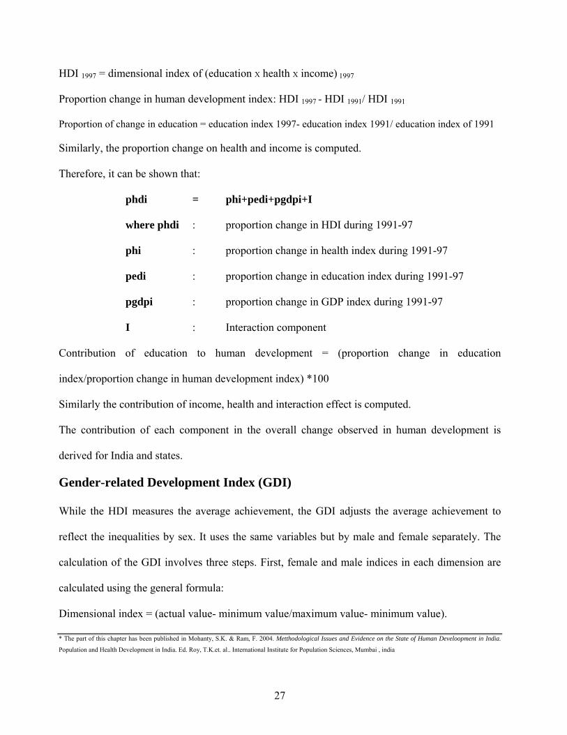
3.2 Decomposition of HDI

We have made an attempt to decompose the change in HDI by each component. For

decomposition we assume a multiplicative model. We compute the changes in HDI as follows.

HDI 1991 = dimensional index of (education X health X income) 1991

27

HDI 1997 = dimensional index of (education X health X income) 1997

Proportion change in human development index: HDI 1997 - HDI 1991/ HDI 1991

Proportion of change in education = education index 1997- education index 1991/ education index of 1991

Similarly, the proportion change on health and income is computed.

Therefore, it can be shown that:

phdi = phi+pedi+pgdpi+I

where phdi : proportion change in HDI during 1991-97

phi : proportion change in health index during 1991-97

pedi : proportion change in education index during 1991-97

pgdpi : proportion change in GDP index during 1991-97

I : Interaction component

Contribution of education to human development = (proportion change in education

index/proportion change in human development index) *100

Similarly the contribution of income, health and interaction effect is computed.

The contribution of each component in the overall change observed in human development is

derived for India and states.

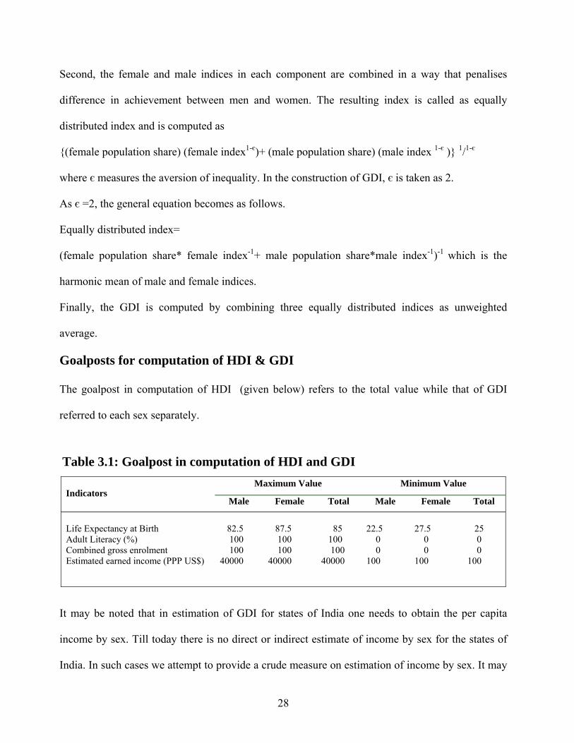
Gender-related Development Index (GDI)

While the HDI measures the average achievement, the GDI adjusts the average achievement to

reflect the inequalities by sex. It uses the same variables but by male and female separately. The

calculation of the GDI involves three steps. First, female and male indices in each dimension are

calculated using the general formula:

Dimensional index = (actual value- minimum value/maximum value- minimum value).

* The part of this chapter has been published in Mohanty, S.K. & Ram, F. 2004. Metthodological Issues and Evidence on the State of Human Develoopment in India.

Population and Health Development in India. Ed. Roy, T.K.et. al.. International Institute for Population Sciences, Mumbai , india

28

Second, the female and male indices in each component are combined in a way that penalises

difference in achievement between men and women. The resulting index is called as equally

distributed index and is computed as

{(female population share) (female index1-є)+ (male population share) (male index 1-є )} 1/1-є

where є measures the aversion of inequality. In the construction of GDI, є is taken as 2.

As є =2, the general equation becomes as follows.

Equally distributed index=

(female population share* female index-1+ male population share*male index-1)-1 which is the

harmonic mean of male and female indices.

Finally, the GDI is computed by combining three equally distributed indices as unweighted

average.

Goalposts for computation of HDI & GDI

The goalpost in computation of HDI (given below) refers to the total value while that of GDI

referred to each sex separately.

Table 3.1: Goalpost in computation of HDI and GDI Maximum Value Minimum Value

Indicators Male Female Total Male Female Total

Life Expectancy at Birth Adult Literacy (%) Combined gross enrolment Estimated earned income (PPP US$)

82.5 100 100 40000

87.5 100 100 40000

85 100 100 40000

22.5 0 0 100

27.5 0 0 100

25 0 0 100

It may be noted that in estimation of GDI for states of India one needs to obtain the per capita

income by sex. Till today there is no direct or indirect estimate of income by sex for the states of

India. In such cases we attempt to provide a crude measure on estimation of income by sex. It may

29

be mentioned that this method is just an illustrative and further modification on methodology may

be made. Our main purpose is to provide the GDI and so we used the estimate for that purpose.

The estimation on per capita income by sex is based on following assumptions.

1. There is no wage differential by sex

2. Difference in income is due to difference in economically active work participation.

At the macro level the male and female share in income may be computed as below.

Female share in wage = proportion of female worker* state domestic product

Female per capita income = female share in wage/ total female population

With these two assumptions we have computed the proportion of male and female workers

among total workers in 2001. We have assumed that the proportion of workers in 2001 to be the

same as in 1997. We then multiply the proportion of female workers with total state domestic

product (SDP) to get the female share. Similarly, we interpolate the population of 1997 from that

of 2001. The sex ratio of 2001 is used to obtain the total population by sex. The female share by

total female population gives the per capita income of females. In the same way the per capita

income is derived for males. It may be noted that the latest provisional estimates of SDP available

corresponds to 1997-98 and so it is used in this paper.

3.3 Economic development in India and states

The economic performance of the country is examined with the help of key macro economic

aggregates such as growth rate of GDP, total food production, foreign exchange reserve, fiscal

deficit, annual rate of inflation and per capita income for the period 1990-2002. The growth rate of

the economy during 1992-93 and 1999-2000 was close to 6.5 percent. The growth rate in the

30

agricultural sector is reflected in total food grain production. The balance of payment has

substantially improved and there is large foreign exchange reserve in recent years. Inflation had

come down from 12.1 percent in 1990-91 to 3.3 percent in 1999-2000. Compared with the record

of the first 40 years of development there is very little doubt that the Indian economy is stronger

than before (Jalan, 2002). However major critics against the liberalisation process mainly focus on

rising unemployment, growing disparities in the income level among the states, higher fiscal

deficit and lack of development in social infrastructure. It is true that the growth rate in recent

years has not generated adequate employment and some states are performing very poorly on the

economic front.

To understand the degree of regional disparity in development, economic performance with

respect to three indicators namely, state domestic product per capita (SDPP), percentage of

population living below poverty line and total number of foreign direct investments (FDI) has been

assessed and given in table 3.2. The data is given for two points of time namely, 1993-94 and

1997-98. It may be noted that the state domestic product per capita (SDPP) is usually considered

as the barometer of economic progress for the state. A higher SDPP reflects higher level of

economic progress and vice versa. However, the SDPP may be affected by three factors namely,

price change, population growth and real economic growth. First, price change can be adjusted by

converting the SDPP into a constant price. In this paper the SDPP for the year 1990-91 and 1997-

98 are converted to 1993-94 prices to make them comparable. The second factor is population

growth, which may be due to both migration, and natural growth (births and deaths). Assuming

that interstate migration is insignificant, the higher the natural growth, the lower will be the growth

of SDPP. The most important factor is the real economic progress due to industrial and agricultural

development. Higher the growth rate in industrial and agricultural production, the higher is likely

31

the growth rate of SDPP. It may be noted that the highest increase in SDPP in 1990s is

experienced in the state of Kerala followed by Tamil Nadu. On the other hand, the states of Bihar

and Assam had registered a negative growth rate in SDPP. This is really a puzzling situation. If the

reporting of SDPP is correct, the low or negative growth rate of SDPP may be attributed to high

population growth and low economic growth in these states.

On the basis of ranking of the states on the SDPP, it may be found that five states namely,

Maharashtra, Punjab, Haryana, Gujarat and Tamil Nadu had a per capita income above the

national average in 1991 and all these states were also above the national average in 1997. On the

other hand, two states namely, Bihar and Orissa remain at the lowest level of economic

development. The economic reforms have not helped the poor performing states to speed up their

economic development. However, the state of Punjab ranked first in 1990-91 but slipped to second

place in 1997-98. Meanwhile, the state of Maharashtra, which had ranked third in SDPP in 1990-

91 ranked first in 1997-98. If we relate this to the number of foreign direct investments it may be

seen that the maximum number of foreign direct investments (FDI) during the period was in

Maharashtra followed by Gujarat whereas state like Bihar had received the minimum number of

investments. The magnitude also differs and gives an approximation on the pattern of foreign

direct investment in the country. This indicates that real economic development is closely related

to industrial development. Thus, economic reform has not helped to reduce the regional disparity

in industrial development. Low economic progress is also accompanied by a high incidence of

poverty in the state. The percentage of population living below the poverty line is highest in Orissa

followed by Bihar. States such as Bihar, Orissa, Uttar Pradesh, Madhya Pradesh and Rajasthan

with low economic development, high incidence of poverty, slow social development needs to

focus on reducing the population growth rate. It is also puzzling to see that the state of

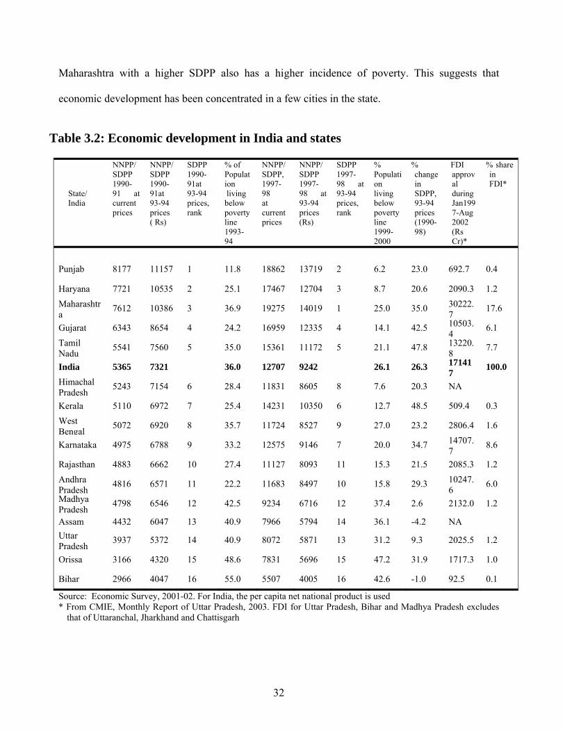
32

Maharashtra with a higher SDPP also has a higher incidence of poverty. This suggests that

economic development has been concentrated in a few cities in the state.

Table 3.2: Economic development in India and states

State/ India

NNPP/SDPP 1990-91 at current prices

NNPP/SDPP 1990-91at 93-94 prices ( Rs)

SDPP 1990-91at 93-94 prices, rank

% of Population living below poverty line 1993-94

NNPP/ SDPP, 1997-98 at current prices

NNPP/SDPP 1997-98 at 93-94 prices (Rs)

SDPP 1997-98 at 93-94 prices, rank

% Population living below poverty line 1999-2000

% change in SDPP, 93-94 prices (1990-98)

FDI approval during Jan1997-Aug 2002 (Rs Cr)*

% share in FDI*

Punjab

8177

11157

1

11.8

18862

13719

2

6.2

23.0

692.7

0.4

Haryana 7721 10535 2 25.1 17467 12704 3 8.7 20.6 2090.3 1.2 Maharashtra

7612 10386 3 36.9 19275 14019 1 25.0 35.0 30222.7

17.6

Gujarat 6343 8654 4 24.2 16959 12335 4 14.1 42.5 10503.4

6.1 Tamil Nadu

5541 7560 5 35.0 15361 11172 5 21.1 47.8 13220.8

7.7

India 5365 7321 36.0 12707 9242 26.1 26.3 171417

100.0 Himachal Pradesh

5243 7154 6 28.4 11831 8605 8 7.6 20.3 NA

Kerala 5110 6972 7 25.4 14231 10350 6 12.7 48.5 509.4 0.3 West Bengal

5072 6920 8 35.7 11724 8527 9 27.0 23.2 2806.4 1.6

Karnataka 4975 6788 9 33.2 12575 9146 7 20.0 34.7 14707.7

8.6

Rajasthan 4883 6662 10 27.4 11127 8093 11 15.3 21.5 2085.3 1.2 Andhra Pradesh

4816 6571 11 22.2 11683 8497 10 15.8 29.3 10247.6

6.0 Madhya Pradesh

4798 6546 12 42.5 9234 6716 12 37.4 2.6 2132.0 1.2

Assam 4432 6047 13 40.9 7966 5794 14 36.1 -4.2 NA Uttar Pradesh

3937 5372 14 40.9 8072 5871 13 31.2 9.3 2025.5 1.2

Orissa 3166 4320 15 48.6 7831 5696 15 47.2 31.9 1717.3 1.0

Bihar 2966 4047 16 55.0 5507 4005 16 42.6 -1.0 92.5 0.1

Source: Economic Survey, 2001-02. For India, the per capita net national product is used * From CMIE, Monthly Report of Uttar Pradesh, 2003. FDI for Uttar Pradesh, Bihar and Madhya Pradesh excludes

that of Uttaranchal, Jharkhand and Chattisgarh

33

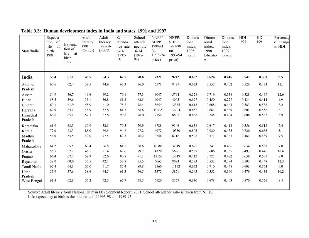
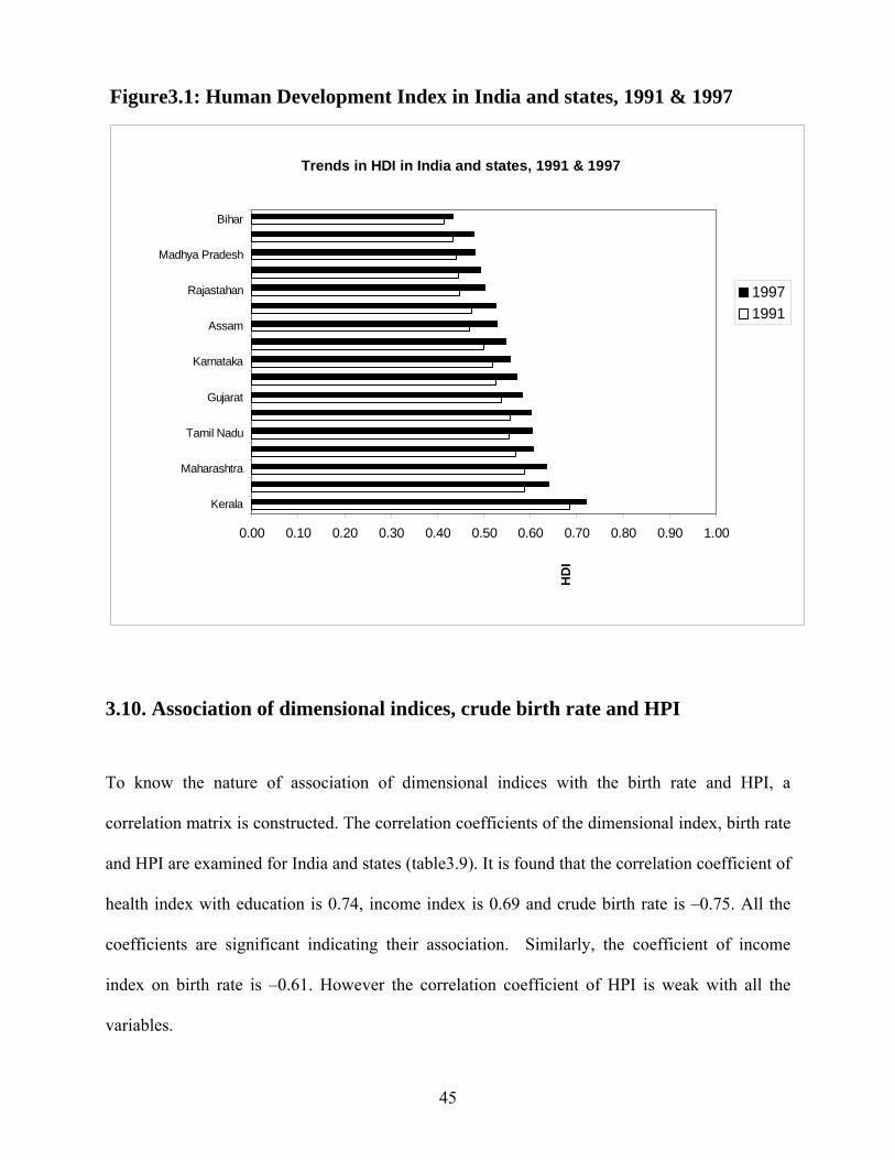
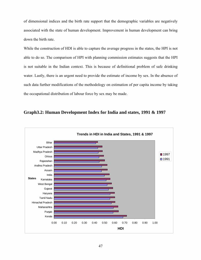
3.4. Levels and trends of human development in India and states

We had initiated the proposition that the link between economic growth and human development is

not automatic. Economic growth is the means and human development is the ultimate end. It may

so happen that a state/country may grow well with regard to economic development but not so in

other dimensions of human development. It was also stated that the average progress in human

development conceals large disparities in the level of development within the country. To start

with, the trend in the human development index for the country has shown a rising trend (Graph

3.2). The levels and trends in human development are examined for the 16 states of India by

computing the HDI at two point of time in 1990s. All the data in the initial period refer to the year

1991 while the latest period refers to the availability of data from different sources. In general, the

latest period may approximate to the year 1997. The variables in the computation of the HDI are

given in table 3.3. The HDI is comparable, as we have used a uniform methodology. The estimated

value of HDI for the country was 0.55, which is very close to the estimates of UNDP, 1997. The

level of human development in 1997 was highest in the state of Kerala with an index value of 0.72

and was lowest in the state of Bihar with an index value of 0.43. If we classify the states as below

and above national average then the states are:

States above national average: Kerala, Maharashtra, Punjab, Himachal Pradesh, Tamil Nadu,

Haryana, Gujarat, West Bengal, Karnataka

States below national average: Assam. Andhra Pradesh, Rajasthan, Orissa, Madhya Pradesh,

Uttar Pradesh and Bihar

The levels of HDI support the previous discussion on large interstate disparities in the level of

development. The values of HDI for the period 1991 and 1997 also indicate the growing inequality

34

in the level of human development among the states. The states which were performing poorly in

the composite indices in 1991 could not improve remarkably even in 1997. The change in HDI

during the period ranges from 0.02 to 0.06. However, with respect to change in HDI, the country

has experienced 10 percent increase. While the maximum change is observed in Assam (13 per

cent) followed by Rajasthan (12 per cent), the minimum change is observed for the state of Bihar

(5 per cent).

35

Table 3.3: Human development index in India and states, 1991 and 1997

Source: Adult literacy from National Human Development Report, 2001, School attendance ratio is taken from NFHS Life expectancy at birth is the mid period of 1993-98 and 1989-93

State/India

Expectation of life at birth 1991

Expectation of life at birth 1995

Adult literacy 1991 (Census)

Adult literacy 1995-56 (NSSO)

School attendance rate 6-14 (1992-93)

School attendance rate 6-14 (1998-99)

NNPP/ SDPP 1990-91 (at 1993-94 price)

NNPP/SDPP 1997-98 (at 1993-94 price)

Dimensional index, 1995 health

Dimensional index, 1998 Education

Dimensional index, 1997 income

HDI 1997

HDI 1991

Percentage changein HDI

India 59.4 61.1 48.5 54.3 67.5 78.6 7321 9242 0.602 0.624 0.416 0.547 0.500 9.5

Andhra Pradesh

60.6 62.4 38.5 44.9 63.3 76.0 6571 8497 0.623 0.552 0.402 0.526 0.473 11.1

Assam 54.9 56.7 49.6 69.2 70.1 77.3 6047 5794 0.528 0.719 0.338 0.528 0.469 12.6 Bihar 58.5 59.6 35.1 36.8 51.3 62.5 4047 4005 0.577 0.450 0.227 0.434 0.414 4.9 Gujarat 60.1 61.9 55.9 61.0 75.7 78.4 8654 12335 0.615 0.668 0.464 0.583 0.538 8.2 Haryana 62.9 64.1 48.9 57.8 81.3 88.6 10535 12704 0.652 0.681 0.469 0.601 0.556 8.1 Himachal Pradesh

63.6 65.1 57.3 62.8 90.8 98.0 7154 8605 0.668 0.745 0.404 0.606 0.567 6.9

Karnataka 61.9 63.3 50.9 52.5 70.5 79.9 6788 9146 0.638 0.617 0.414 0.556 0.518 7.4 Kerala 72.0 73.3 88.0 89.5 94.8 97.2 6972 10350 0.805 0.920 0.435 0.720 0.685 5.1 Madhya Pradesh

54.0 55.5 40.0 47.5 62.3 76.2 6546 6716 0.508 0.571 0.363 0.481 0.439 9.5

Maharashtra 64.2 65.5 60.4 66.8 81.5 88.6 10386 14019 0.675 0.741 0.486 0.634 0.588 7.8 Orissa 55.5 57.2 46.1 51.4 69.6 79.2 4320 5696 0.537 0.606 0.335 0.493 0.446 10.6 Punjab 66.4 67.7 52.9 62.6 80.8 91.1 11157 13719 0.712 0.721 0.482 0.638 0.587 8.8 Rajasthan 58.0 60.0 35.5 42.1 58.8 75.5 6662 8093 0.583 0.532 0.394 0.503 0.448 12.3 Tamil Nadu 62.4 64.1 57.0 61.7 82.4 89.8 7560 11172 0.652 0.710 0.448 0.603 0.554 9.0 Uttar Pradesh

55.9 57.6 38.6 44.5 61.3 76.5 5372 5871 0.543 0.552 0.340 0.479 0.434 10.2

West Bengal 61.5 62.8 56.2 62.5 67.7 78.5 6920 8527 0.630 0.678 0.403 0.570 0.526 8.5

36

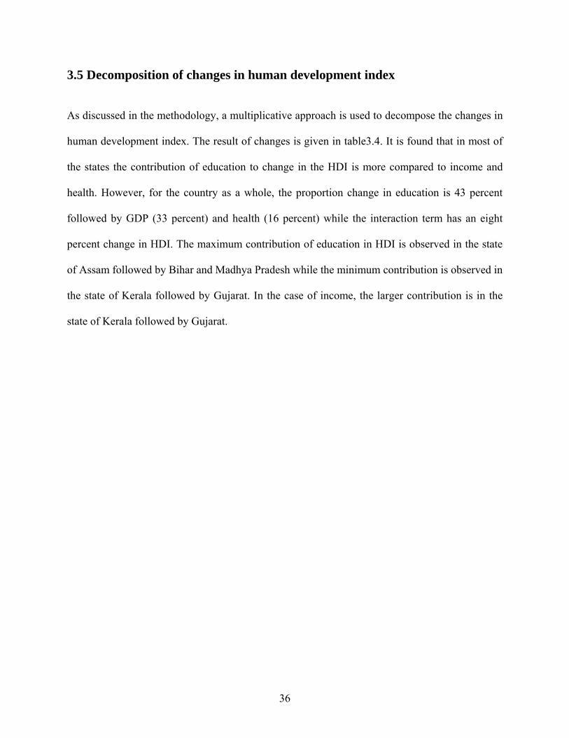
3.5 Decomposition of changes in human development index

As discussed in the methodology, a multiplicative approach is used to decompose the changes in

human development index. The result of changes is given in table3.4. It is found that in most of

the states the contribution of education to change in the HDI is more compared to income and

health. However, for the country as a whole, the proportion change in education is 43 percent

followed by GDP (33 percent) and health (16 percent) while the interaction term has an eight

percent change in HDI. The maximum contribution of education in HDI is observed in the state

of Assam followed by Bihar and Madhya Pradesh while the minimum contribution is observed in

the state of Kerala followed by Gujarat. In the case of income, the larger contribution is in the

state of Kerala followed by Gujarat.

37

Table 3.4: Decomposition of human development index, 1991 -97 State/India

HDI, HDI 1991 1997

Proportion change in HDI health education income

Interaction effect

Percentage contribution of Health Education Income Interaction

India 0.119 0.156 0.317 0.049 0.138 0.103 0.027 15.6 43.4 32.5 8.5 Andhra Pradesh 0.100 0.139 0.389 0.051 0.181 0.119 0.038 13.0 46.6 30.7 9.7 Assam 0.097 0.128 0.323 0.060 0.274 -0.021 0.009 18.6 84.9 -6.4 2.9 Bihar 0.063 0.072 0.139 0.033 0.109 -0.006 0.003 23.7 78.8 -4.5 1.9 Gujarat 0.148 0.191 0.288 0.051 0.069 0.146 0.022 17.8 24.1 50.6 7.5 Haryana 0.165 0.208 0.260 0.032 0.140 0.071 0.017 12.2 53.9 27.4 6.5 Himachal Pradesh 0.164 0.201 0.225 0.039 0.089 0.083 0.014 17.3 39.6 36.8 6.4 Karnataka 0.129 0.163 0.266 0.038 0.073 0.136 0.018 14.3 27.5 51.3 6.9 Kerala 0.261 0.322 0.235 0.028 0.020 0.179 0.009 11.8 8.4 76.0 3.9 Madhya Pradesh 0.082 0.105 0.280 0.052 0.203 0.012 0.014 18.5 72.4 4.2 4.9 Maharashtra 0.192 0.243 0.266 0.033 0.099 0.115 0.019 12.5 37.2 43.2 7.1 Orissa 0.079 0.109 0.376 0.056 0.124 0.160 0.037 14.8 33.0 42.4 9.8 Punjab 0.192 0.247 0.288 0.031 0.159 0.077 0.020 10.9 55.3 26.8 7.0 Rajasthan 0.086 0.122 0.421 0.061 0.230 0.090 0.041 14.4 54.5 21.3 9.8 Tamil Nadu 0.156 0.207 0.328 0.045 0.085 0.170 0.027 13.9 26.0 52.0 8.2 Uttar Pradesh 0.077 0.102 0.318 0.055 0.195 0.046 0.023 17.3 61.3 14.3 7.1 West Bengal 0.133 0.172 0.296 0.049 0.148 0.077 0.023 16.5 49.9 25.9 7.7

38

3.6 Gender differential in income by sex in India and states

Gender issues in general and gender discrimination in particular are matters of great concern for

the country. The gender differential in the key area of human development can be the starting

point to look into the issues. The gender disparity in the areas of education, health and income is

reflected from various censuses and surveys. For example, in 2001 there were 126 of 591

districts, which had a female literacy of less than 40 percent compared to only one district where

male literacy is below 40 percent (Ram and Mohanty, 2001). At the same time, the age specific

death rate (ASDR) in many states is higher for females compared to males till age 29 (SRS,

1998). The declining sex ratio of the 0-6 populations is a reflection of the attitude of our society

toward the girl child. Though it is difficult to quantify all types of discrimination with respect to

sex, an approximation at the aggregate level can be made from construction of composite

indices. The GDI as developed by UNDP adjusts the differentials in key areas of human

development. However, the main difficulty in the construction of such indices is the non-

availability of data on income by sex. This is probably the reason why many researchers and

organizations could not construct such an index at the state level in India. To overcome this

difficulty we have attempted to derive an indirect estimate of income by sex and then used the

estimated income for construction of GDI.

In this section we have provided the indirect estimate of income by sex for the states of

India. The estimates of per capita income is provided for the year 1997-98 and expressed at

1997-98 prices. As discussed before, we have taken the proportion of workers as the base in this

exercise. The proportions of male and female workers as in 2001 are given in table 3.5. Among

total workers, male workers were 68 percent and female workers were 32 percent. Assuming that

there is no wage differential in income among males and females, it is logical that the female

share in SDPP will be the proportion of female workers multiplied by total SDPP. For the

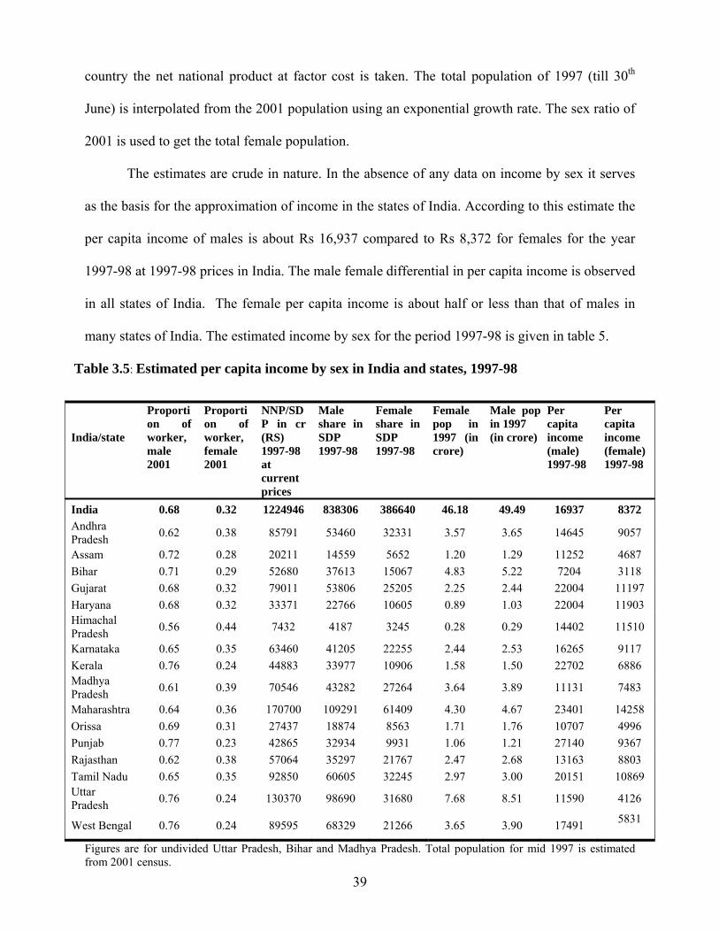
39

country the net national product at factor cost is taken. The total population of 1997 (till 30th

June) is interpolated from the 2001 population using an exponential growth rate. The sex ratio of

2001 is used to get the total female population.

The estimates are crude in nature. In the absence of any data on income by sex it serves

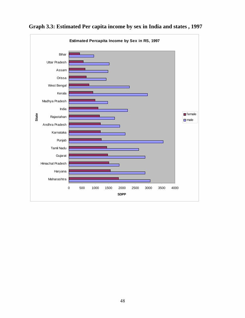
as the basis for the approximation of income in the states of India. According to this estimate the

per capita income of males is about Rs 16,937 compared to Rs 8,372 for females for the year

1997-98 at 1997-98 prices in India. The male female differential in per capita income is observed

in all states of India. The female per capita income is about half or less than that of males in

many states of India. The estimated income by sex for the period 1997-98 is given in table 5.

Table 3.5: Estimated per capita income by sex in India and states, 1997-98

India/state

Proportion of worker, male 2001

Proportion of worker, female 2001

NNP/SDP in cr (RS) 1997-98 at current prices

Male share in SDP 1997-98

Female share in SDP 1997-98

Female pop in 1997 (in crore)

Male pop in 1997 (in crore)

Per capita income (male) 1997-98

Per capita income (female) 1997-98

India 0.68 0.32 1224946 838306 386640 46.18 49.49 16937 8372 Andhra Pradesh 0.62 0.38 85791 53460 32331 3.57 3.65 14645 9057

Assam 0.72 0.28 20211 14559 5652 1.20 1.29 11252 4687 Bihar 0.71 0.29 52680 37613 15067 4.83 5.22 7204 3118 Gujarat 0.68 0.32 79011 53806 25205 2.25 2.44 22004 11197 Haryana 0.68 0.32 33371 22766 10605 0.89 1.03 22004 11903 Himachal Pradesh 0.56 0.44 7432 4187 3245 0.28 0.29 14402 11510

Karnataka 0.65 0.35 63460 41205 22255 2.44 2.53 16265 9117 Kerala 0.76 0.24 44883 33977 10906 1.58 1.50 22702 6886 Madhya Pradesh 0.61 0.39 70546 43282 27264 3.64 3.89 11131 7483

Maharashtra 0.64 0.36 170700 109291 61409 4.30 4.67 23401 14258 Orissa 0.69 0.31 27437 18874 8563 1.71 1.76 10707 4996 Punjab 0.77 0.23 42865 32934 9931 1.06 1.21 27140 9367 Rajasthan 0.62 0.38 57064 35297 21767 2.47 2.68 13163 8803 Tamil Nadu 0.65 0.35 92850 60605 32245 2.97 3.00 20151 10869 Uttar Pradesh 0.76 0.24 130370 98690 31680 7.68 8.51 11590 4126

West Bengal 0.76 0.24 89595 68329 21266 3.65 3.90 17491 5831

Figures are for undivided Uttar Pradesh, Bihar and Madhya Pradesh. Total population for mid 1997 is estimated from 2001 census.

40

3.7. Gender–related development index for India and states, 1997

The HDI measures the average progress while the GDI reflects the inequalities in human

development by sex. It may so happen that one state may perform better in HDI but not so with

respect to sex. Here the input variables are specified by sex. Besides estimated income, the life

expectancy at birth by sex, adult literacy and school attendance rate of children in the age group

6-14 are given in table 3.6. For India, the estimated value of GDI is 0.556, very close to the

estimate of UNDP for 1999 (0.553). It may be mentioned that the difference in HDI and GDI

rank for the year 1999 was –1 for India (UNDP, HDR 2001). The GDI value is highest in the

state of Kerala followed by Maharashtra and Punjab. There are differentials in the values of HDI

and GDI among the states indicating that the gender differential in human development is

prevalent in all the states. A comparison of HDI and GDI values is discussed in the next section.

41

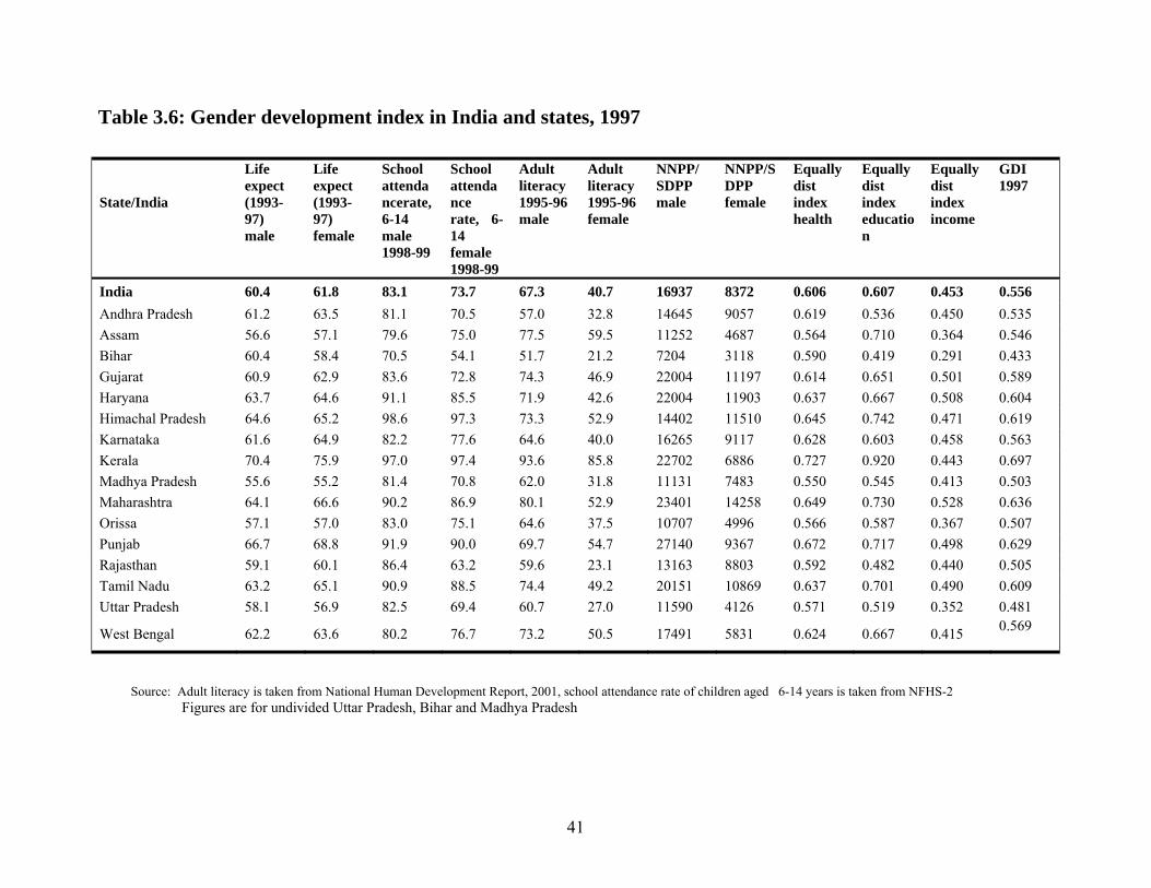
Table 3.6: Gender development index in India and states, 1997

Source: Adult literacy is taken from National Human Development Report, 2001, school attendance rate of children aged 6-14 years is taken from NFHS-2 Figures are for undivided Uttar Pradesh, Bihar and Madhya Pradesh

State/India

Life expect (1993-97) male

Life expect (1993-97) female

School attendancerate, 6-14 male 1998-99

School attendance rate, 6-14 female 1998-99

Adult literacy 1995-96 male

Adult literacy1995-96 female

NNPP/ SDPP male

NNPP/SDPP female

Equally dist index health

Equally dist index education

Equally dist index income

GDI 1997

India 60.4 61.8 83.1 73.7 67.3 40.7 16937 8372 0.606 0.607 0.453 0.556 Andhra Pradesh 61.2 63.5 81.1 70.5 57.0 32.8 14645 9057 0.619 0.536 0.450 0.535 Assam 56.6 57.1 79.6 75.0 77.5 59.5 11252 4687 0.564 0.710 0.364 0.546 Bihar 60.4 58.4 70.5 54.1 51.7 21.2 7204 3118 0.590 0.419 0.291 0.433 Gujarat 60.9 62.9 83.6 72.8 74.3 46.9 22004 11197 0.614 0.651 0.501 0.589 Haryana 63.7 64.6 91.1 85.5 71.9 42.6 22004 11903 0.637 0.667 0.508 0.604 Himachal Pradesh 64.6 65.2 98.6 97.3 73.3 52.9 14402 11510 0.645 0.742 0.471 0.619 Karnataka 61.6 64.9 82.2 77.6 64.6 40.0 16265 9117 0.628 0.603 0.458 0.563 Kerala 70.4 75.9 97.0 97.4 93.6 85.8 22702 6886 0.727 0.920 0.443 0.697 Madhya Pradesh 55.6 55.2 81.4 70.8 62.0 31.8 11131 7483 0.550 0.545 0.413 0.503 Maharashtra 64.1 66.6 90.2 86.9 80.1 52.9 23401 14258 0.649 0.730 0.528 0.636 Orissa 57.1 57.0 83.0 75.1 64.6 37.5 10707 4996 0.566 0.587 0.367 0.507 Punjab 66.7 68.8 91.9 90.0 69.7 54.7 27140 9367 0.672 0.717 0.498 0.629 Rajasthan 59.1 60.1 86.4 63.2 59.6 23.1 13163 8803 0.592 0.482 0.440 0.505 Tamil Nadu 63.2 65.1 90.9 88.5 74.4 49.2 20151 10869 0.637 0.701 0.490 0.609 Uttar Pradesh 58.1 56.9 82.5 69.4 60.7 27.0 11590 4126 0.571 0.519 0.352 0.481

West Bengal 62.2 63.6 80.2 76.7 73.2 50.5 17491 5831 0.624 0.667 0.415 0.569

42

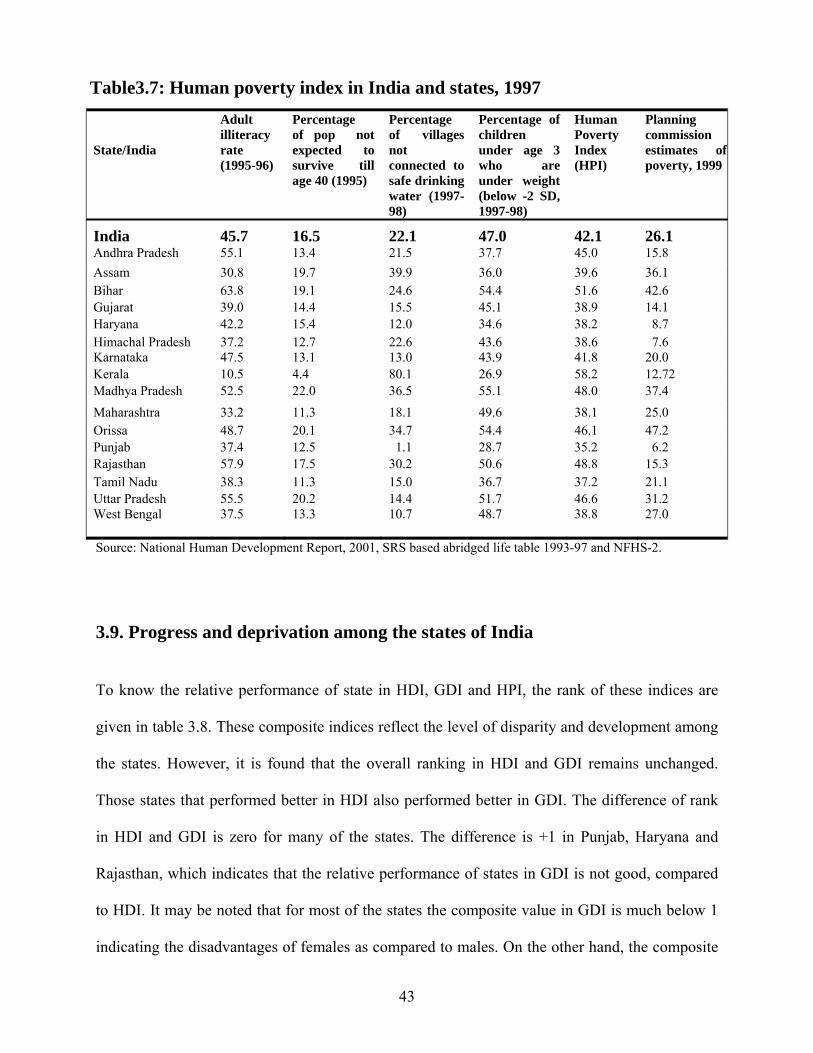
3.8. Human poverty index in India and states, 1997

Human development can also be measured with respect to deprivation and one way of doing so

is through the human poverty index. While the HDI measures the achievement in the average

progress, the human poverty index measures the deprivation in human development. The

variables used in the construction of HPI are education measured by percent of adult illiterate,

economic progress measured by unweighted average of the percent of population not having

access to safe drinking water and health measured by the percentage of children under age five

who are underweight. The HPI is usually used for developing countries and computed as one

third of the cube root of cube of each dimension. This indicates that the dimension in which

deprivation is more will get a higher weight and vice versa. In this paper we have derived the

illiteracy rate from NSSO, 1997-98 while the SRS based abridged life table is used to find out

the percentage of population not surviving to age 40. The percent of children under age three

who are underweight (percentage below –2 SD) is taken from NFHS-2. Similarly, the percent of

households not connected with piped water and hand pump is used for unsafe drinking water is

also taken from NFHS-2.

The estimates of HPI are very hard to believe. If the HPI-1 captures human deprivation,

then the value of HPI should be close to that of planning commission estimates on poverty. For

the national level the HPI is 42.1which is much above the planning commission estimates on

poverty of 26 percent. Even the state of Kerala, which ranks first in HDI and GDI, also has a

higher value of HPI. Even if we exclude the state of Kerala because of high value for lack of

access to safe drinking, the HPI estimate is inconsistent with the planning commission estimate

in most of the states. For example, the difference of HPI and planning commission estimates is

about 29 points in Punjab and Andhra Pradesh. Thus, on the basis of the above it may be said

that the HPI is not a suitable measure in the Indian context.

43

Table3.7: Human poverty index in India and states, 1997 State/India

Adult illiteracy rate (1995-96)

Percentage of pop not expected to survive till age 40 (1995)

Percentage of villages not connected to safe drinking water (1997-98)

Percentage of children under age 3 who are under weight (below -2 SD, 1997-98)

Human Poverty Index (HPI)

Planning commission estimates of poverty, 1999

India 45.7 16.5 22.1 47.0 42.1 26.1 Andhra Pradesh 55.1 13.4 21.5 37.7 45.0 15.8 Assam 30.8 19.7 39.9 36.0 39.6 36.1 Bihar 63.8 19.1 24.6 54.4 51.6 42.6 Gujarat 39.0 14.4 15.5 45.1 38.9 14.1 Haryana 42.2 15.4 12.0 34.6 38.2 8.7 Himachal Pradesh 37.2 12.7 22.6 43.6 38.6 7.6 Karnataka 47.5 13.1 13.0 43.9 41.8 20.0 Kerala 10.5 4.4 80.1 26.9 58.2 12.72 Madhya Pradesh 52.5 22.0 36.5 55.1 48.0 37.4 Maharashtra 33.2 11.3 18.1 49.6 38.1 25.0 Orissa 48.7 20.1 34.7 54.4 46.1 47.2 Punjab 37.4 12.5 1.1 28.7 35.2 6.2 Rajasthan 57.9 17.5 30.2 50.6 48.8 15.3 Tamil Nadu 38.3 11.3 15.0 36.7 37.2 21.1 Uttar Pradesh 55.5 20.2 14.4 51.7 46.6 31.2 West Bengal 37.5 13.3 10.7 48.7 38.8 27.0

Source: National Human Development Report, 2001, SRS based abridged life table 1993-97 and NFHS-2.

3.9. Progress and deprivation among the states of India

To know the relative performance of state in HDI, GDI and HPI, the rank of these indices are

given in table 3.8. These composite indices reflect the level of disparity and development among

the states. However, it is found that the overall ranking in HDI and GDI remains unchanged.

Those states that performed better in HDI also performed better in GDI. The difference of rank

in HDI and GDI is zero for many of the states. The difference is +1 in Punjab, Haryana and

Rajasthan, which indicates that the relative performance of states in GDI is not good, compared

to HDI. It may be noted that for most of the states the composite value in GDI is much below 1

indicating the disadvantages of females as compared to males. On the other hand, the composite

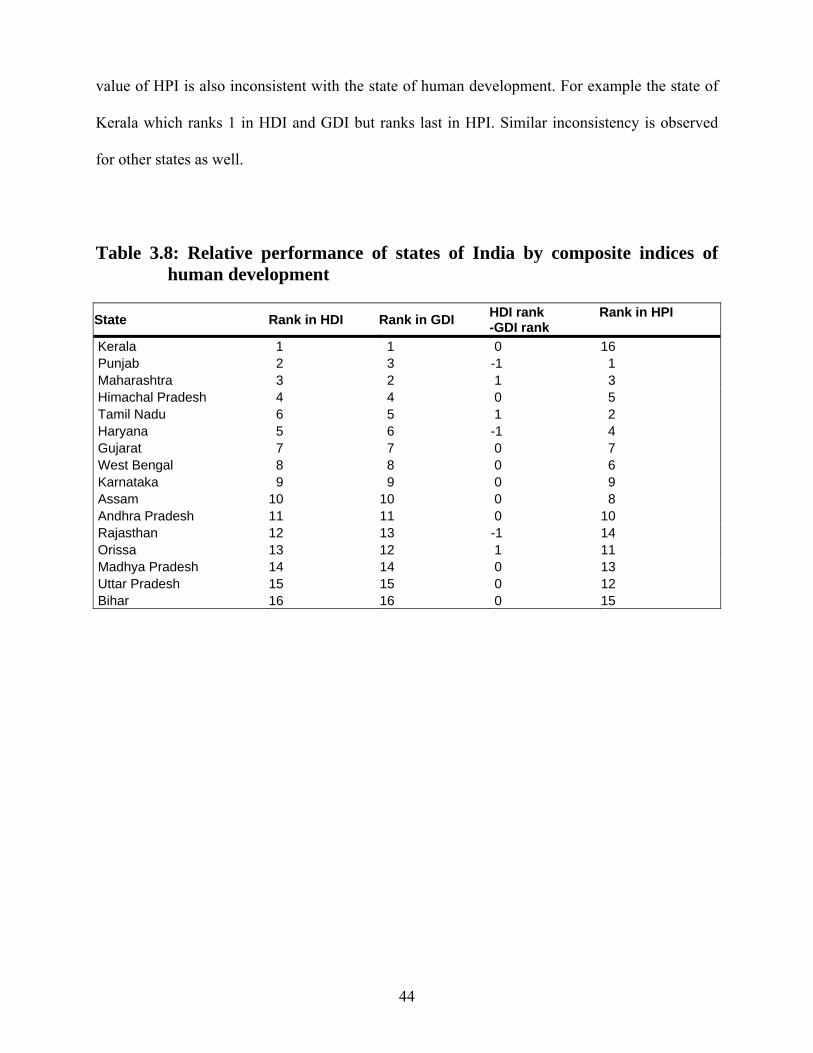
44

value of HPI is also inconsistent with the state of human development. For example the state of

Kerala which ranks 1 in HDI and GDI but ranks last in HPI. Similar inconsistency is observed

for other states as well.

Table 3.8: Relative performance of states of India by composite indices of

human development State Rank in HDI Rank in GDI HDI rank Rank in HPI

-GDI rank Kerala 1 1 0 16 Punjab 2 3 -1 1 Maharashtra 3 2 1 3 Himachal Pradesh 4 4 0 5 Tamil Nadu 6 5 1 2 Haryana 5 6 -1 4 Gujarat 7 7 0 7 West Bengal 8 8 0 6 Karnataka 9 9 0 9 Assam 10 10 0 8 Andhra Pradesh 11 11 0 10 Rajasthan 12 13 -1 14 Orissa 13 12 1 11 Madhya Pradesh 14 14 0 13 Uttar Pradesh 15 15 0 12 Bihar 16 16 0 15

45

Figure3.1: Human Development Index in India and states, 1991 & 1997

Trends in HDI in India and states, 1991 & 1997

0.00 0.10 0.20 0.30 0.40 0.50 0.60 0.70 0.80 0.90 1.00

Kerala

Maharashtra

Tamil Nadu

Gujarat

Karnataka

Assam

Rajastahan

Madhya Pradesh

Bihar

HD

I

19971991

3.10. Association of dimensional indices, crude birth rate and HPI

To know the nature of association of dimensional indices with the birth rate and HPI, a

correlation matrix is constructed. The correlation coefficients of the dimensional index, birth rate

and HPI are examined for India and states (table3.9). It is found that the correlation coefficient of

health index with education is 0.74, income index is 0.69 and crude birth rate is –0.75. All the

coefficients are significant indicating their association. Similarly, the coefficient of income

index on birth rate is –0.61. However the correlation coefficient of HPI is weak with all the

variables.

46

Table3.9: Correlation matrix of dimensional indices, HPI and birth rate

Variables Dimensional index on education 1997

Dimensional index on income 1997

Dimensional index on health 1997

Birth rate, 1999

HPI, 1997

Dimensional index on education 1997 Dimensional index on income 1997 Dimensional index on health 1997 Birth rate, 1999 HPI, 1997

1 0.74** 0.69** -0.75** -0.05

1 0.6* -0.72* 0.24

1 -0.61** -.32

1 0.13

1

N= 17 * p < 0.05, ** p < .01

3.11. Conclusion

From the above discussion it may be stated India and the states have experienced improvement

in the state of human development. The country has achieved higher economic growth, improved

the balance of payments position and achieved price stability. But this development has not been

accompanied by a growth in employment. The implication is that with rising population, the

greatest challenge in the coming years will be to provide employment opportunities for a

growing labour force. The second important finding is the large interstate disparity not only in

economic development but also in human development as well. The states, which are

economically better off, performed well in human development while the states, which were at

the bottom of economic progress, also had a low level of human development. The SDPP and the

composite indices such as HDI, GDI and HPI support the argument. The correlation coefficients

47

of dimensional indices and the birth rate support that the demographic variables are negatively

associated with the state of human development. Improvement in human development can bring

down the birth rate.

While the construction of HDI is able to capture the average progress in the states, the HPI is not

able to do so. The comparison of HPI with planning commission estimates suggests that the HPI

is not suitable in the Indian context. This is because of definitional problem of safe drinking

water. Lastly, there is an urgent need to provide the estimate of income by sex. In the absence of

such data further modifications of the methodology on estimation of per capita income by taking

the occupational distribution of labour force by sex may be made.

Graph3.2: Human Development Index for India and states, 1991 & 1997

Trends in HDI in India and States, 1991 & 1997

0.00 0.10 0.20 0.30 0.40 0.50 0.60 0.70 0.80 0.90 1.00

Kerala

Punjab

Maharashtra

Himachal Pradesh

Tamil Nadu

Haryana

Gujarat

West Bengal

Karnataka

India

Assam

Andhra Pradesh

Rajastahan

Orissa

Madhya Pradesh

Uttar Pradesh

Bihar

HDI

States

19971991

48

Graph 3.3: Estimated Per capita income by sex in India and states , 1997

Estimated Percapita Income by Sex in RS, 1997

0 500 1000 1500 2000 2500 3000 3500 4000

Maharashtra

Haryana

Himachal Pradesh

Gujarat

Tamil Nadu

Punjab

Karnataka

Andhra Pradesh

Rajastahan

India

Madhya Pradesh

Kerala

West Bengal

Orissa

Assam

Uttar Pradesh

Bihar

Stat

e

SDPP

female

male