Embed Size (px)
Citation preview
Department of Physics/College of Education (UOM) 2012-2013 Electromagnetic Theory/4th Class
صباحية والمسائيةالدراسات ال 1
Chapter three
Electrostatic Boundary Value Problems
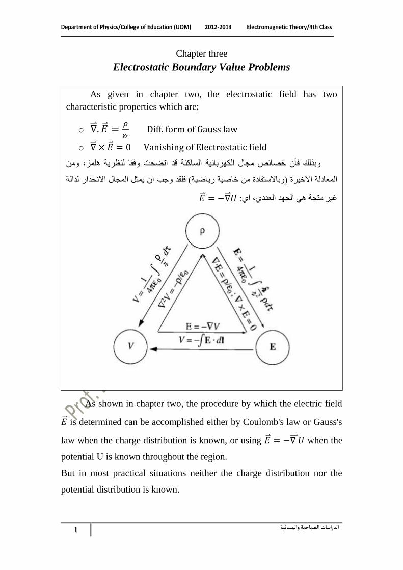
As shown in chapter two, the procedure by which the electric field
�⃑� is determined can be accomplished either by Coulomb's law or Gauss's
law when the charge distribution is known, or using �⃑� = −∇ ⃑⃑⃑ 𝑈 when the
potential U is known throughout the region.
But in most practical situations neither the charge distribution nor the
potential distribution is known.
As given in chapter two, the electrostatic field has two
characteristic properties which are;
o ∇⃑⃑ . �⃑� =𝜌
𝜀° Diff. form of Gauss law
o ∇⃑⃑ × �⃑� = 0 Vanishing of Electrostatic field
وبذلك فأن خصائص مجال الكهربائية الساكنة قد اتضحت وفقا لنظرية هلمز، ومن
المعادلة االخيرة )وباالستفادة من خاصية رياضية( فلقد وجب ان يمثل المجال االنحدار لدالة
= �⃑�غير متجة هي الجهد العددي، اي: −∇⃑⃑ 𝑈

Department of Physics/College of Education (UOM) 2012-2013 Electromagnetic Theory/4th Class
صباحية والمسائيةالدراسات ال 2
In this chapter, we shall consider practical electrostatic problems where
only electrostatic conditions (charge and potential) at some boundaries are
known and it's desired to find �⃑� and U throughout the region. Such
problems, however, are usually solved by Poisson's or Laplace's equation.
3-1 Poisson's Equation معادلة بواسون
Poisson's and also Laplace's equation are easily derived from Gauss's
low for a linear medium. It has been shown in previous chapter that Gauss's
low can be expressed as;
∇⃑⃑ . �⃑⃑� = ∇⃑⃑ . (𝜖�⃑� ) = 𝜌 … (2 − 26)
Also, it is proved that
�⃑� = −∇⃑⃑ 𝑈 … (2 − 10)
Substituting equation (2-10) in(2-26) yields ;
∇⃑⃑ . 𝜖(−∇⃑⃑ 𝑈) = 𝜌 (3 − 1)
For a homogenous medium equation (3-1) becomes;
𝛁𝟐 𝑼 = −𝝆
𝝐 … (3 − 2)
Equation (3-2) called Poisson's equation.
3-2 Laplace's Equation معادلة البالس
In fact Laplace's equation is a special case for Poisson's equation
which occurs when the region under consideration being free from charge
(i.e. = 0 ). Thus equation (3-2) becomes;
𝛁𝟐𝑼 = 𝟎 … (𝟑 − 𝟑)
Last equation is Laplace's equation for homogenous medium.
For an inhomogeneous medium the Laplace's equation is equation
(3-1) when the right-hand side vanishes (𝜌 = 0).
According to ideas of chapter one, Laplace's equation in Cartesian,
cylindrical and spherical coordinates respectively is given by;
Department of Physics/College of Education (UOM) 2012-2013 Electromagnetic Theory/4th Class
صباحية والمسائيةالدراسات ال 3
𝜕2𝑈
𝜕𝑥2+
𝜕2𝑈
𝜕𝑦2+
𝜕2𝑈
𝜕𝑧2= 0 . . . (3 − 3)
1
𝑟
𝜕
𝜕𝑟(𝑟
𝜕𝑈
𝜕𝑟) +
1
𝑟2
𝜕𝑈
𝜕𝜑2+
𝜕2𝑈
𝜕𝑧2= 0 . . . (3 − 4)
1
𝑟2
𝜕
𝜕𝑟(𝑟2
𝜕𝑈
𝜕𝑟) +
1
𝑟2 sin 𝜃 𝜕
𝜕𝜃(𝑠𝑖𝑛𝜃
𝜕𝑈
𝜕𝜃) +
1
𝑟2 sin2 𝜃
𝜕𝑈
𝜕𝜑2= 0 . . (3 − 5)
Depending on whether the potential is 𝑈(𝑥 , 𝑦 , 𝑧), 𝑈(𝑟 , 𝜑, 𝑧) and
𝑈(𝑟, 𝜃, 𝜑 ).
Laplace's equation is of primary importance is solving electrostatic
problems, involving a set of conductors material at different potentials.
Examples of such problems include capacitors and vacuum tube diode.
H.W:
Find the mathematical form of Poisson's equation in Cartesian,
cylindrical and spherical coordinates.
3-3: Laplace's Equation Solution in One Dimension:
3-3-1: Cartesian Coordinates
∇2𝑈 = 0
𝜕2𝑈
𝜕𝑥2+
𝜕2𝑈
𝜕𝑦2+
𝜕2𝑈
𝜕𝑧2= 0
𝜕2𝑈
𝜕𝑥2= 0
𝑑2𝑈
𝑑𝑥2= 0
𝑑
𝑑𝑥(𝑑𝑈
𝑑𝑥) = 0
𝑑𝑈
𝑑𝑥= 𝑎
𝑈 = 𝑎 ∫𝑑𝑥
Department of Physics/College of Education (UOM) 2012-2013 Electromagnetic Theory/4th Class
صباحية والمسائيةالدراسات ال 4
𝑈(𝑥) = 𝑎𝑥 + 𝑏 . . . (3 − 6)
Where 𝑎 and 𝑏 are constants to be determined according to the
imposed boundary condition. Equation (3-6) describe equipotential
surfaces which are plate located at 𝑥 = constant.
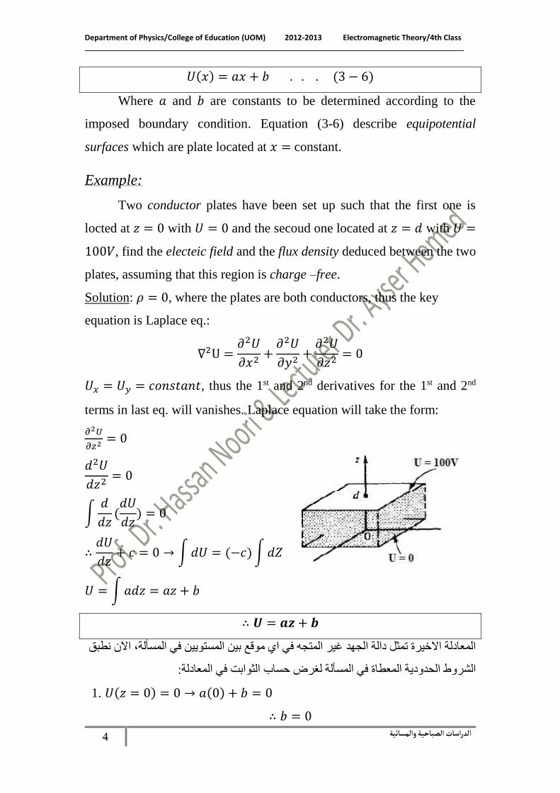
Example:
Two conductor plates have been set up such that the first one is
locted at 𝑧 = 0 with 𝑈 = 0 and the secoud one located at 𝑧 = 𝑑 with 𝑈 =
100𝑉, find the electeic field and the flux density deduced between the two
plates, assuming that this region is charge –free.
Solution: 𝜌 = 0, where the plates are both conductors, thus the key
equation is Laplace eq.:
∇2U =𝜕2𝑈
𝜕𝑥2+
𝜕2𝑈
𝜕𝑦2+
𝜕2𝑈
𝜕𝑧2= 0
𝑈𝑥 = 𝑈𝑦 = 𝑐𝑜𝑛𝑠𝑡𝑎𝑛𝑡, thus the 1st and 2nd derivatives for the 1st and 2nd
terms in last eq. will vanishes. Laplace equation will take the form:
𝜕2𝑈
𝜕𝑧2= 0
𝑑2𝑈
𝑑𝑧2= 0
∫𝑑
𝑑𝑧(𝑑𝑈
𝑑𝑧) = 0
∴𝑑𝑈
𝑑𝑧+ 𝑐 = 0 → ∫𝑑𝑈 = (−𝑐)∫𝑑𝑍
𝑈 = ∫𝑎𝑑𝑧 = 𝑎𝑧 + 𝑏
∴ 𝑼 = 𝒂𝒛 + 𝒃
المعادلة االخيرة تمثل دالة الجهد غير المتجه في اي موقع بين المستويين في المسألة، االن نطبق
الشروط الحدودية المعطاة في المسألة لغرض حساب الثوابت في المعادلة:
1. 𝑈(𝑧 = 0) = 0 → 𝑎(0) + 𝑏 = 0
∴ 𝑏 = 0
Department of Physics/College of Education (UOM) 2012-2013 Electromagnetic Theory/4th Class
صباحية والمسائيةالدراسات ال 5
2. 𝑈(𝑧 = 𝑑) = 100 → 𝑎(𝑑) + 𝑏 = 100
∴ 𝑎 =100
𝑑
Thus: U(z) = (100
𝑑) z
االن لحساب دالة المجال بين اللوحين باالستفادة من المعادلة االخيرة، نطبق العالقة التبادلية بين
الجهد والمجال )الصيغة التفاضلية للجهد(:
�⃑� = −∇⃑⃑ U
لالحداثيات المتعامدة في مسألتنا:
�⃑� = − {𝜕𝑈
𝜕𝑥�̂� +
𝜕𝑈
𝜕𝑦𝑗̂ +
𝜕𝑈
𝜕𝑧�̂�}
= −𝜕
𝜕𝑧(100
𝑧
𝑑) �̂�
= −100
𝑑�̂� (𝑉/𝑚)
لحساب كثافة الفيض:
�⃑⃑� = 𝜖�⃑�
∴ �⃑⃑� = −1000
𝑑𝜖�̂� (𝐶/𝑚2)
Where; at the first plate:
𝐷𝑛 = −𝜖100
𝑑(
𝑐
𝑚2)
𝐷𝑛 = +𝜖100
𝑑(
𝑐
𝑚2) at the second plate.(why?)
3-3-2 Cylindrical Coordinate:
As an example assume that 𝑈 is a function only for 𝑟, i.e.
𝑈(𝑟, 𝜑, 𝑧) = 𝑈(𝑟). For this case Laplce's equation given in equation (3-4)
reduces to the form;

Department of Physics/College of Education (UOM) 2012-2013 Electromagnetic Theory/4th Class
صباحية والمسائيةالدراسات ال 6
1
𝑟 𝜕
𝜕𝑟(𝑟
𝜕𝑈
𝜕𝑟) = 0
→1
𝑟 𝑑
𝑑𝑟(𝑟
𝑑𝑈
𝑑𝑟) = 0
∫𝑑
𝑑𝑟(𝑟
𝑑𝑈
𝑑𝑟) = 0
∴ 𝑟𝑑𝑈
𝑑𝑟= 𝑎
𝑑𝑈
𝑑𝑟= 𝑎𝑟−1 → ∫𝑑𝑈 = 𝑎 ∫
𝑑𝑟
𝑟
𝑈 = ∫𝑎
𝑟𝑑𝑟 = 𝑎 ln 𝑟 + 𝑏
∴ 𝑈(𝑟) = 𝑎 ln 𝑟 + 𝑏 . . . (3 − 7)
Equation (3-7) describe an equipotential surfaces which are cylinders of
𝑟 = constant.
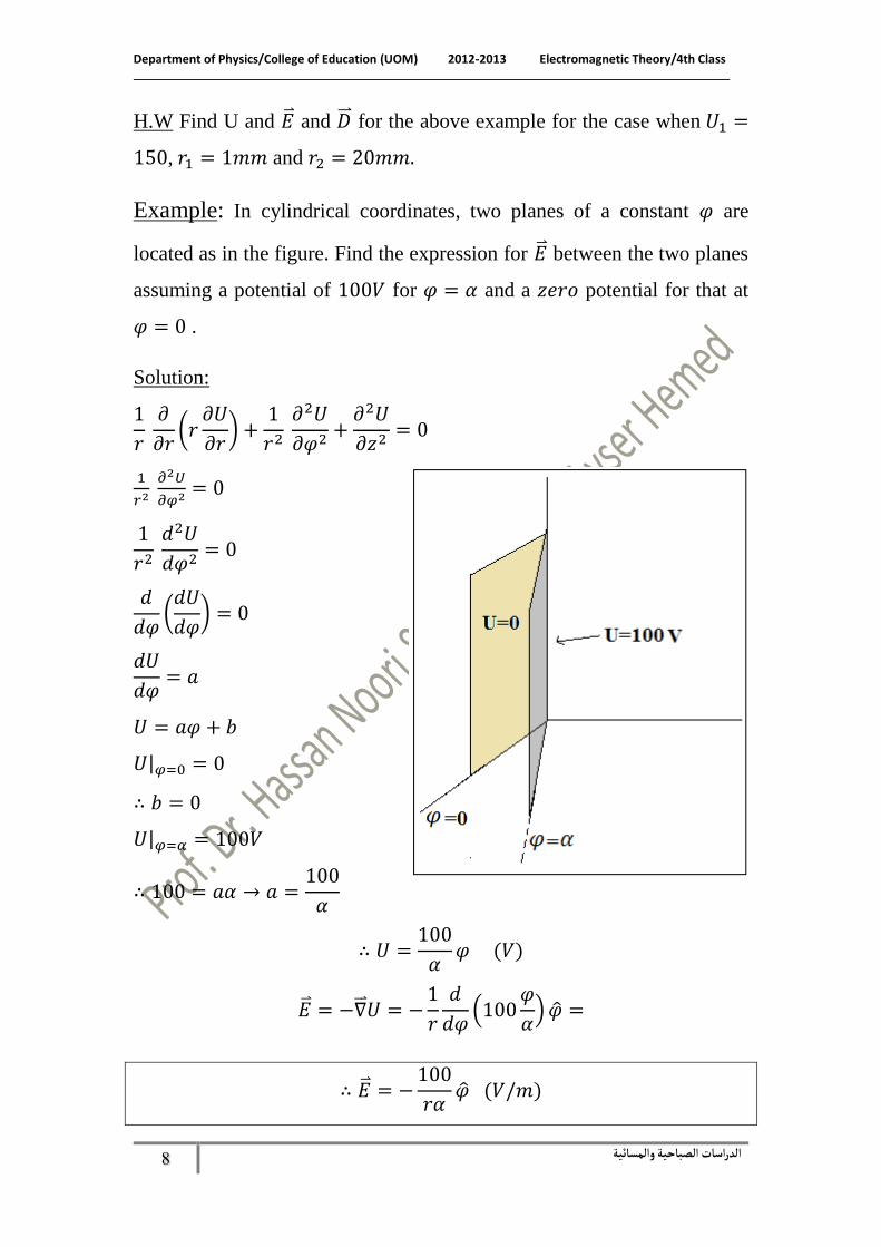
Example: Find the potential function and the electric field intensity for
the region between two concentric right circular cylinders, where 𝑈 = 𝑈1
at 𝑟 = 𝑟1 and 𝑈 = 0 at 𝑟 = 𝑟2, where 𝑟2 > 𝑟1.
Solution: the potantial is cons. with 𝜑 and z,
Laplace equation reduces to:
1
𝑟 𝜕
𝜕𝑟(𝑟
𝜕𝑈
𝜕𝑟) = 0
𝑈(𝑟) = 𝑎 ln 𝑟 + 𝑏
Applying the boundary conditions;
1. 1.𝑈(𝑟2) = 𝑎 ln 𝑟2 + 𝑏 = 0
𝑏 = −𝑎 ln( 𝑟2)
2. 𝑈(𝑟1) = 𝑎 ln(𝑟1) − 𝑎 ln(𝑟2) = 𝑈1

Department of Physics/College of Education (UOM) 2012-2013 Electromagnetic Theory/4th Class
صباحية والمسائيةالدراسات ال 7
𝑎 (ln (𝑟1𝑟2
)) = 𝑈1
∴ 𝑎 =𝑈1
ln (𝑟1𝑟2
)
∴ 𝑏 = −𝑈1
ln (𝑟1𝑟2
) . ln ( 𝑟2)
→ 𝑈(𝑟) =𝑈1
ln (𝑟1𝑟2
) . ln ( 𝑟) −
𝑈1
ln (𝑟1𝑟2
) . ln ( 𝑟2)
=𝑈1
ln (𝑟1𝑟2
){ln ( 𝑟) − ln ( 𝑟2)}
𝑈(𝑟) =𝑈1
ln (𝑟1𝑟2
)ln (
𝑟
𝑟2)
�⃑� = −∇⃑⃑ 𝑈
= −{𝜕𝑈
𝜕𝑟�̂� +
1
𝑟
𝜕𝑈
𝜕𝜑�̂� +
𝜕𝑈
𝜕𝑧�⃑� }
= −𝑑𝑈
𝑑𝑟�̂�
= −𝑑
𝑑𝑟{
𝑈1
ln (𝑟1𝑟2
)ln (
𝑟
𝑟2)} �̂�
= −𝑈1
ln (𝑟1𝑟2
) .
𝑑
𝑑𝑟ln (
𝑟
𝑟2) �̂�
= −𝑈1
ln (𝑟1𝑟2
) .
1
𝑟 𝑟2⁄ .
1
𝑟2�̂�
∴ �⃑� = −𝑈1
ln (𝑟1𝑟2
) .�̂�
𝑟
Department of Physics/College of Education (UOM) 2012-2013 Electromagnetic Theory/4th Class
صباحية والمسائيةالدراسات ال 8
H.W Find U and �⃑� and �⃑⃑� for the above example for the case when 𝑈1 =
150, 𝑟1 = 1𝑚𝑚 and 𝑟2 = 20𝑚𝑚.
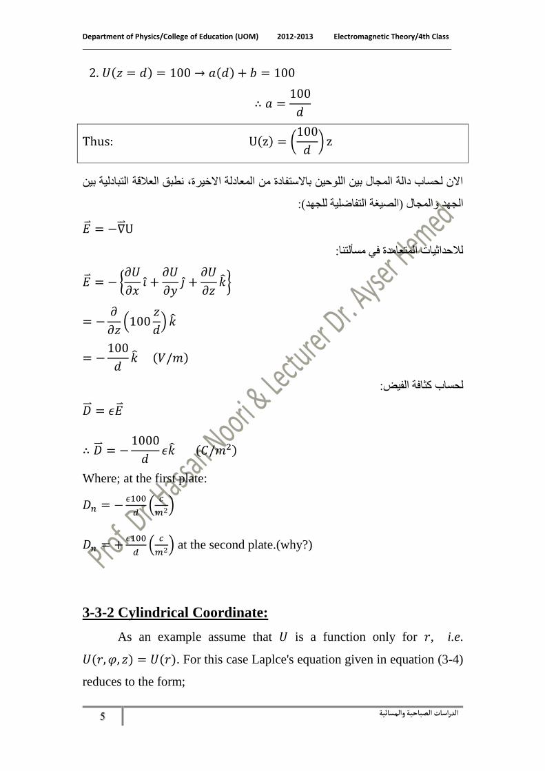
Example: In cylindrical coordinates, two planes of a constant 𝜑 are
located as in the figure. Find the expression for �⃑� between the two planes
assuming a potential of 100𝑉 for 𝜑 = 𝛼 and a 𝑧𝑒𝑟𝑜 potential for that at
𝜑 = 0 .
Solution:
1
𝑟 𝜕
𝜕𝑟(𝑟
𝜕𝑈
𝜕𝑟) +
1
𝑟2 𝜕2𝑈
𝜕𝜑2+
𝜕2𝑈
𝜕𝑧2= 0
1
𝑟2 𝜕2𝑈
𝜕𝜑2= 0
1
𝑟2 𝑑2𝑈
𝑑𝜑2= 0
𝑑
𝑑𝜑(𝑑𝑈
𝑑𝜑) = 0
𝑑𝑈
𝑑𝜑= 𝑎
𝑈 = 𝑎𝜑 + 𝑏
𝑈|𝜑=0 = 0
∴ 𝑏 = 0
𝑈|𝜑=𝛼 = 100𝑉
∴ 100 = 𝑎𝛼 → 𝑎 =100
𝛼
∴ 𝑈 =100
𝛼𝜑 (𝑉)
�⃑� = −∇⃑⃑ 𝑈 = −1
𝑟
𝑑
𝑑𝜑(100
𝜑
𝛼) �̂� =
∴ �⃑� = −100
𝑟𝛼�̂� (𝑉/𝑚)
Department of Physics/College of Education (UOM) 2012-2013 Electromagnetic Theory/4th Class
صباحية والمسائيةالدراسات ال 9
3-3-3 Spherical coordinates:
Laplace's equation in this coordinates is written as in equation (3-5).
∇2𝑈 =1
𝑟2 𝜕
𝜕𝑟(𝑟2
𝜕𝑈
𝜕𝑟) +
1
𝑟2 𝑠𝑖𝑛𝜃
𝜕
𝜕𝜃(𝑠𝑖𝑛𝜃
𝜕𝑈
𝜕𝜃) +
1
𝑟2 𝑠𝑖𝑛𝜃
𝜕2𝑈
𝜕𝜑2= 0
. . . (3 − 5)
The equation describes U when it varies with (𝑟, 𝜃 , 𝜑 ). As an example if
we assume that U is vary only with r, i.e. 𝑈(𝑟, 𝜃 , 𝜑 ) = 𝑈(𝑟).
Consequently equation (3-5) reduces to the form;
1
𝑟2 𝑑
𝑑𝑟(𝑟
𝑑𝑈
𝑑𝑟) = 0
𝑑
𝑑𝑟(𝑟
𝑑𝑈
𝑑𝑟) = 0
𝑟𝑑𝑈
𝑑𝑟= 𝑎
𝑑𝑈
𝑑𝑟=
𝑎
𝑟
𝑈 = −𝑎
𝑟+ 𝑏
�⃑� = −�⃑� 𝑈 = −(𝑑𝑈
𝑑𝑟�̂� +
1
𝑟
𝜕𝑈
𝜕𝜃𝜃 +
1
𝑟 𝑠𝑖𝑛𝜃
𝑑𝑈
𝑑𝜑�̂�)
= −𝑑𝑈
𝑑𝑟�̂�
�⃑� =−𝑎
𝑟2�̂�
Department of Physics/College of Education (UOM) 2012-2013 Electromagnetic Theory/4th Class
صباحية والمسائيةالدراسات ال 10
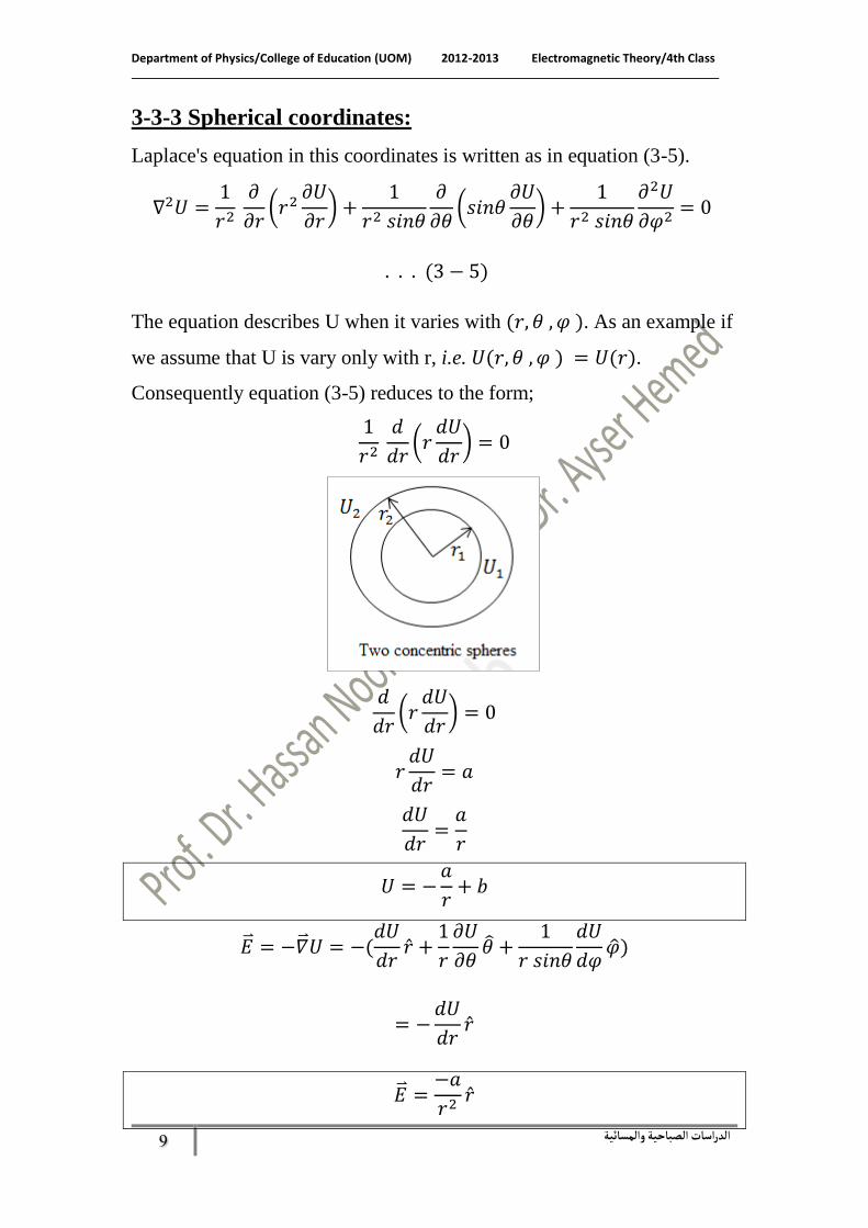
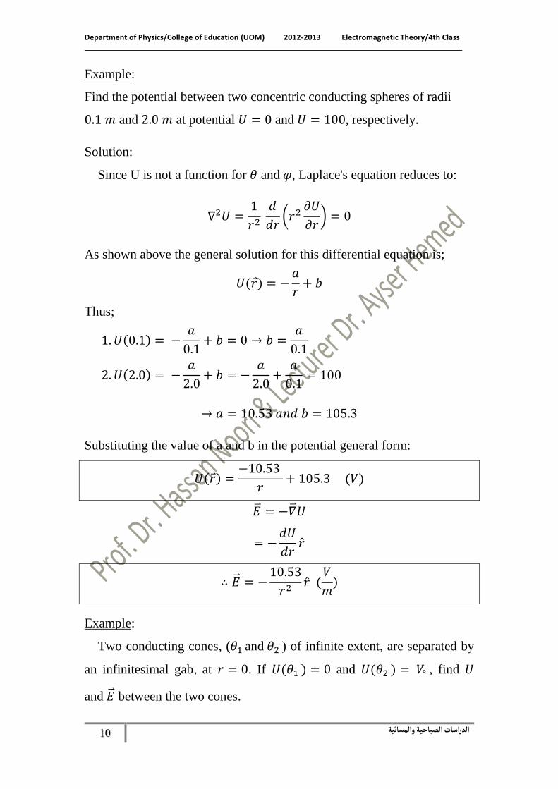
Example:
Find the potential between two concentric conducting spheres of radii
0.1 𝑚 and 2.0 𝑚 at potential 𝑈 = 0 and 𝑈 = 100, respectively.
Solution:
Since U is not a function for 𝜃 and 𝜑, Laplace's equation reduces to:
∇2𝑈 =1
𝑟2 𝑑
𝑑𝑟(𝑟2
𝜕𝑈
𝜕𝑟) = 0
As shown above the general solution for this differential equation is;
𝑈(𝑟 ) = −𝑎
𝑟+ 𝑏
Thus;
1. 𝑈(0.1) = −𝑎
0.1+ 𝑏 = 0 → 𝑏 =
𝑎
0.1
2. 𝑈(2.0) = −𝑎
2.0+ 𝑏 = −
𝑎
2.0+
𝑎
0.1= 100
→ 𝑎 = 10.53 𝑎𝑛𝑑 𝑏 = 105.3
Substituting the value of a and b in the potential general form:
𝑈(𝑟 ) =−10.53
𝑟+ 105.3 (𝑉)
�⃑� = −�⃑� 𝑈
= −𝑑𝑈
𝑑𝑟�̂�
∴ �⃑� = −10.53
𝑟2�̂� (
𝑉
𝑚)
Example:
Two conducting cones, (𝜃1 and 𝜃2 ) of infinite extent, are separated by
an infinitesimal gab, at 𝑟 = 0. If 𝑈(𝜃1 ) = 0 and 𝑈(𝜃2 ) = 𝑉° , find 𝑈
and �⃑� between the two cones.
Department of Physics/College of Education (UOM) 2012-2013 Electromagnetic Theory/4th Class
صباحية والمسائيةالدراسات ال 11
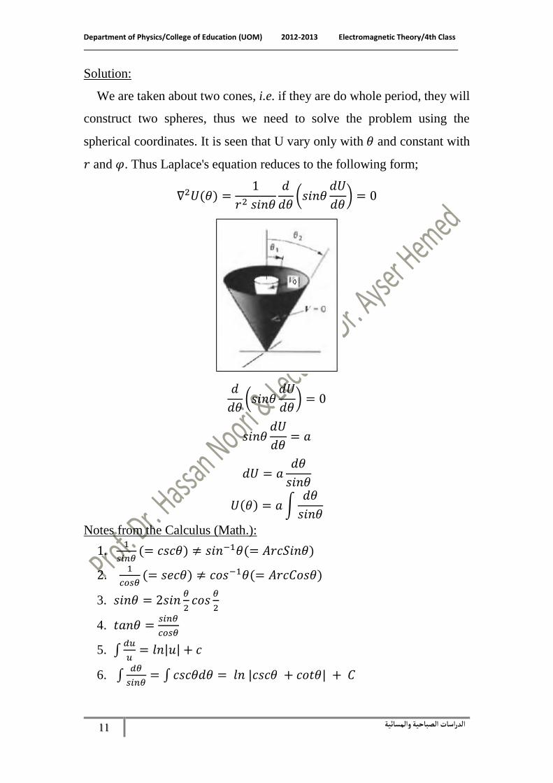
Solution:
We are taken about two cones, i.e. if they are do whole period, they will
construct two spheres, thus we need to solve the problem using the
spherical coordinates. It is seen that U vary only with 𝜃 and constant with
𝑟 and 𝜑. Thus Laplace's equation reduces to the following form;
∇2𝑈(𝜃) =1
𝑟2 𝑠𝑖𝑛𝜃
𝑑
𝑑𝜃(𝑠𝑖𝑛𝜃
𝑑𝑈
𝑑𝜃) = 0
𝑑
𝑑𝜃(𝑠𝑖𝑛𝜃
𝑑𝑈
𝑑𝜃) = 0
𝑠𝑖𝑛𝜃𝑑𝑈
𝑑𝜃= 𝑎
𝑑𝑈 = 𝑎𝑑𝜃
𝑠𝑖𝑛𝜃
𝑈(𝜃) = 𝑎 ∫𝑑𝜃
𝑠𝑖𝑛𝜃
Notes from the Calculus (Math.):
1. 1
𝑠𝑖𝑛𝜃(= 𝑐𝑠𝑐𝜃) ≠ 𝑠𝑖𝑛−1𝜃(= 𝐴𝑟𝑐𝑆𝑖𝑛𝜃)
2. 1
𝑐𝑜𝑠𝜃(= 𝑠𝑒𝑐𝜃) ≠ 𝑐𝑜𝑠−1𝜃(= 𝐴𝑟𝑐𝐶𝑜𝑠𝜃)
3. 𝑠𝑖𝑛𝜃 = 2𝑠𝑖𝑛𝜃
2𝑐𝑜𝑠
𝜃
2
4. 𝑡𝑎𝑛𝜃 =𝑠𝑖𝑛𝜃
𝑐𝑜𝑠𝜃
5. ∫𝑑𝑢
𝑢= 𝑙𝑛|𝑢| + 𝑐
6. ∫𝑑𝜃
𝑠𝑖𝑛𝜃= ∫𝑐𝑠𝑐𝜃𝑑𝜃 = 𝑙𝑛 |𝑐𝑠𝑐𝜃 + 𝑐𝑜𝑡𝜃| + 𝐶

Department of Physics/College of Education (UOM) 2012-2013 Electromagnetic Theory/4th Class
صباحية والمسائيةالدراسات ال 12
∴ 𝑈(𝜃) = 𝑎 ∫𝑑𝜃
2 cos (𝜃2) sin (
𝜃2)
𝑚𝑢𝑙𝑡𝑖𝑝𝑙𝑦 𝑤𝑖𝑡ℎ: 𝑐𝑜𝑠
𝜃2
𝑐𝑜𝑠𝜃2
= 𝑎 ∫
12𝑠𝑒𝑐2(
𝜃2)𝑑𝜃
𝑡𝑎𝑛 (𝜃2)
But: 1
2 𝑠𝑒𝑐2(
𝜃
2) =
𝑑[tan (𝜃
2)]
𝑑𝜃
∴ 𝑈(𝜃) = 𝑎𝑙𝑛 |𝑡𝑎𝑛𝜃
2| + 𝑏 . . . (#)
This equation represents the solution of Laplace equation in spherical
coordinates, in on dimension which is 𝜃.
1. 𝑈( 𝜃1 ) = 𝑎 𝑙𝑛 (𝑡𝑎𝑛𝜃1
2) + 𝑏 = 0
∴ 𝑏 = −𝑎 𝑙𝑛 (𝑡𝑎𝑛𝜃1
2) . . . (1)
2. 𝑈( 𝜃2 ) = 𝑎 𝑙𝑛 (𝑡𝑎𝑛𝜃2
2) + 𝑏 = 𝑉°
𝑜𝑟: 𝑉° = 𝑎 [𝑙𝑛 (𝑡𝑎𝑛𝜃2
2) − 𝑙𝑛 (𝑡𝑎𝑛
𝜃1
2)]
∴ 𝑎 =𝑉°
𝑙𝑛 [𝑡𝑎𝑛
𝜃2
2
𝑡𝑎𝑛𝜃1
2
]
. . . (2)
Sub in eq.1
∴ 𝑏 = −𝑉°𝑙𝑛 (𝑡𝑎𝑛
𝜃1
2 )
𝑙𝑛 [𝑡𝑎𝑛
𝜃2
2
𝑡𝑎𝑛𝜃1
2
]
. . . (3)
Sub. of eqs. 1 and 3 in eq.(#) yield:
𝑈(𝜃) = 𝑉°𝑙𝑛 [𝑡𝑎𝑛
𝜃2
𝑡𝑎𝑛𝜃1
2
] − 𝑉°𝑙𝑛 [𝑡𝑎𝑛
𝜃2
2
𝑡𝑎𝑛𝜃1
2
]
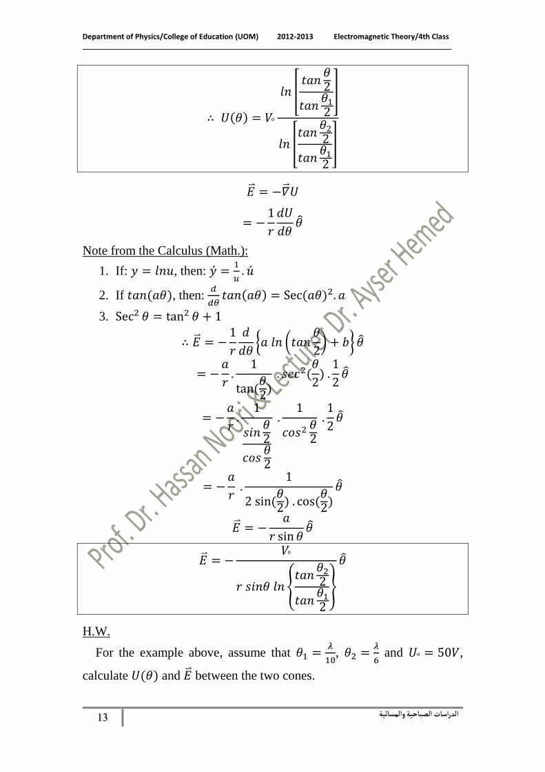
Department of Physics/College of Education (UOM) 2012-2013 Electromagnetic Theory/4th Class
صباحية والمسائيةالدراسات ال 13
∴ 𝑈(𝜃) = 𝑉°
𝑙𝑛 [𝑡𝑎𝑛
𝜃2
𝑡𝑎𝑛𝜃1
2
]
𝑙𝑛 [𝑡𝑎𝑛
𝜃2
2
𝑡𝑎𝑛𝜃1
2
]
�⃑� = −�⃑� 𝑈
= −1
𝑟
𝑑𝑈
𝑑𝜃𝜃
Note from the Calculus (Math.):
1. If: 𝑦 = 𝑙𝑛𝑢, then: �́� =1
𝑢. �́�
2. If 𝑡𝑎𝑛(𝑎𝜃), then: 𝑑
𝑑𝜃𝑡𝑎𝑛(𝑎𝜃) = Sec (𝑎𝜃)2. 𝑎
3. Sec 2 𝜃 = tan 2 𝜃 + 1
∴ �⃑� = −1
𝑟
𝑑
𝑑𝜃{𝑎 𝑙𝑛 (𝑡𝑎𝑛
𝜃
2) + 𝑏} 𝜃
= −𝑎
𝑟.
1
tan (𝜃2) . 𝑠𝑒𝑐2(
𝜃
2) .
1
2𝜃
= −𝑎
𝑟.
1
𝑠𝑖𝑛𝜃2
𝑐𝑜𝑠𝜃2
.1
𝑐𝑜𝑠2 𝜃2
.1
2𝜃
= −𝑎
𝑟 .
1
2 sin (𝜃2) . cos (
𝜃2)𝜃
�⃑� = −𝑎
𝑟 sin 𝜃𝜃
�⃑� = −𝑉°
𝑟 𝑠𝑖𝑛𝜃 𝑙𝑛 {𝑡𝑎𝑛
𝜃2
2
𝑡𝑎𝑛𝜃1
2
}
𝜃
H.W.
For the example above, assume that 𝜃1 =𝜆
10, 𝜃2 =
𝜆
6 and 𝑈° = 50𝑉,
calculate 𝑈(𝜃) and �⃑� between the two cones.
Department of Physics/College of Education (UOM) 2012-2013 Electromagnetic Theory/4th Class
صباحية والمسائيةالدراسات ال 14
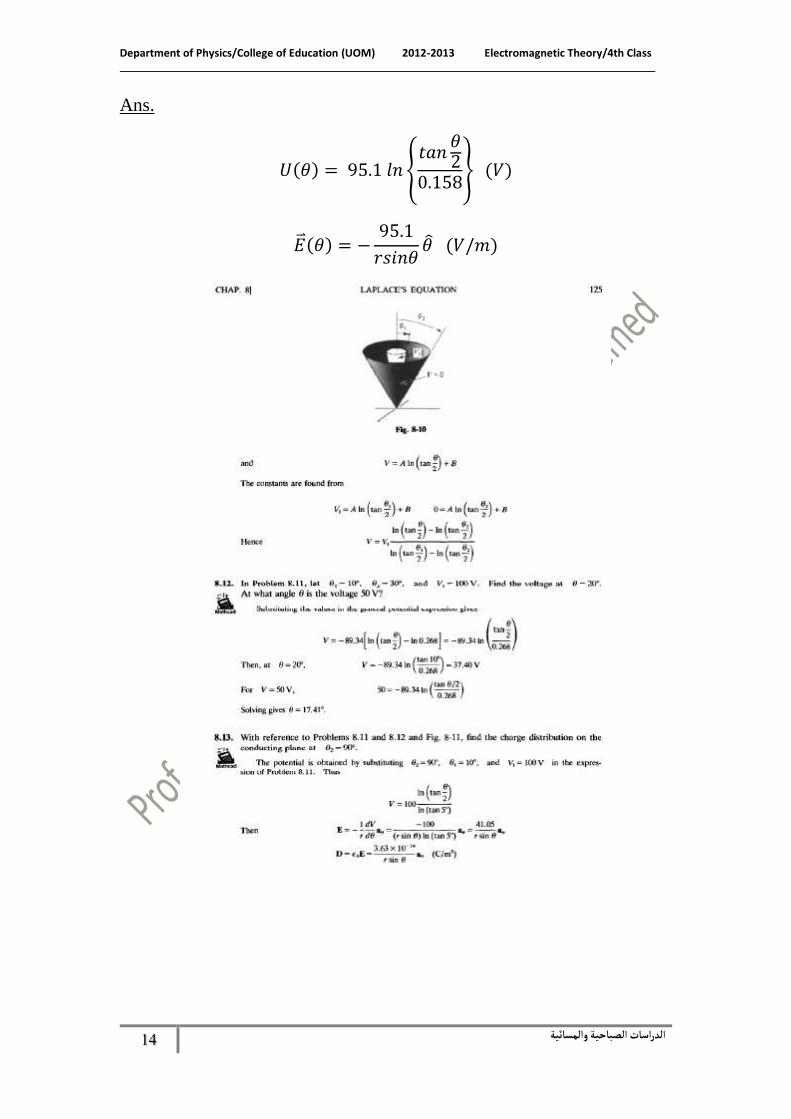
Ans.
𝑈(𝜃) = 95.1 𝑙𝑛 {𝑡𝑎𝑛
𝜃2
0.158} (𝑉)
�⃑� (𝜃) = −95.1
𝑟𝑠𝑖𝑛𝜃𝜃 (𝑉/𝑚)
Department of Physics/College of Education (UOM) 2012-2013 Electromagnetic Theory/4th Class
صباحية والمسائيةالدراسات ال 15
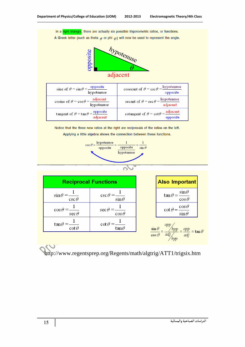
http://www.regentsprep.org/Regents/math/algtrig/ATT1/trigsix.htm


![4. PRACTICAL ELECTROSTATIC MEASUREMENTS 4.pdf · Chapter 4: Practical electrostatic measurements 48 washing of the cargo tanks of large crude oil tankers [7,8] and electrostatic conditions](https://img.pdfslide.us/doc/110x75/5a7a70297f8b9a05348b997f/4-practical-electrostatic-4pdfchapter-4-practical-electrostatic-measurements.jpg)
![Electromagnetic Field Theory [Chapter[Chapter 4 ...edu.hansung.ac.kr/~kwangho/lectures/EMT/2010_Fall/...Electromagnetic Field Theory [Chapter[Chapter 4: Electrostatic Fields] 4: Electrostatic](https://img.pdfslide.us/doc/110x75/610d249c8745b56c264c1390/electromagnetic-field-theory-chapterchapter-4-edu-kwangholecturesemt2010fall.jpg)