Embed Size (px)
Citation preview
Chapter One
Characteristics of Instrumentation
بسم الله الرحمن الرحيم
Objective of the chapter
This chapter presents some of the
fundamental concepts of measurement
in the context of a simple generalized
instrument model.

• An instrument is a device that transforms a
physical variable of interest (the measurand)
into a form that is suitable for recording (the
measurement). • An example of the above definitions Instrument === a ruler measurand === the required lengthmeasurement === 4units === cm

1.1 Simple Instrument Model pp.4
FIGURE 1. Simple Instrument Model .

• In Figure 1, • The sensor: has the function of converting the
physical variable input into a signal variable output.
• Signal variables have the property that they can be manipulated in a transmission system, such as an electrical or mechanical circuit.
• In electrical circuits, voltage is a common signal variable. In mechanical systems, displacement or force are commonly used as signal variables.

Table 1 Physical measurement variables pp.4
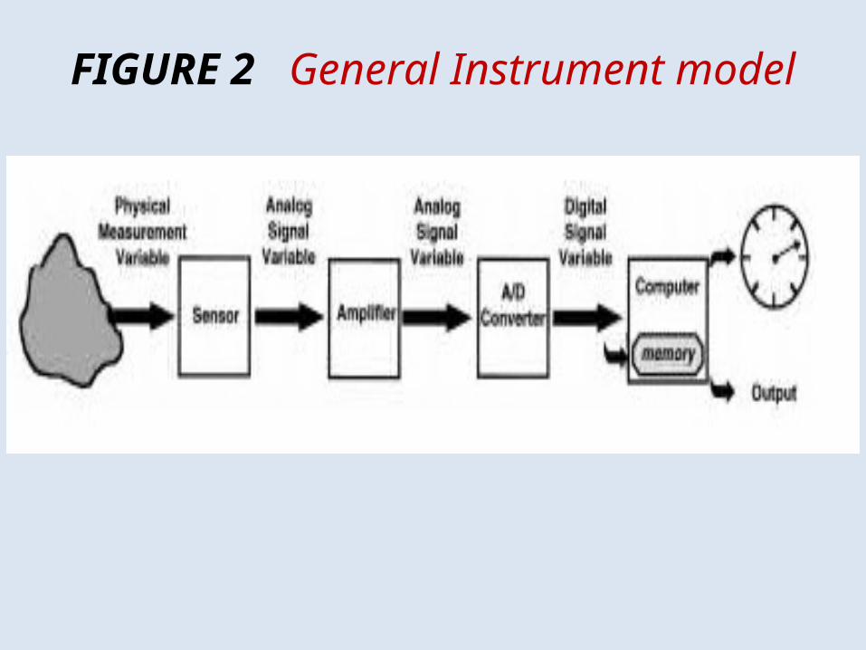
FIGURE 2 General Instrument model

1.2 Passive and Active Sensors
• Passive sensors do not add energy as part of
the measurement process but may remove
energy in their operation.
• One example of a passive sensor is a
thermocouple, which converts a physical
temperature into a voltage signal.

1.2 Passive and Active Sensors
• Active sensors add energy to the measurement environment as part of the measurement process.
• An example of an active sensor is a radar or sonar system, where the distance to some object is measured by actively sending out a radio (radar) or acoustic (sonar) wave to reflect off of some object and measure its range from the sensor.

1.3 Calibration
• The relationship between the physical measurement variable input and the signal variable (output) for a specific sensor is known as the calibration of the sensor.
• A sensor (or an entire instrument system) is calibrated by providing a known physical input to the system and recording the output.

1.3 Calibration
• The sensor has a linear response for values of the physical input less than X0.
• For values of the physical input greater than X0, the calibration curve becomes less sensitive until it reaches a limiting value of the output signal, referred to as saturation,
• The sensor cannot be used for measurements greater than its saturation value

1.3 Calibration
FIGURE 3 Calibration curve example.

1.3 Calibration
• In some cases, the sensor will not respond to very small values of the physical input variable.
• The difference between the smallest and largest physical inputs that can reliably be measured by an instrument determines the dynamic range of the device.

1.4 Modifying and Interfering Inputs
• In some cases, the sensor output will be influenced by physical variables other than the intended measurand. This is called an interfering input
• In Figure 4, X is the intended measurand, Y is an interfering input
• The measured signal output is therefore a combination of X and Y with Y interfering with the intended measurand X.

1.4 Modifying and Interfering Inputs
FIGURE 4 Interfering inputs.

1.4 Modifying and Interfering Inputs
• Modifying inputs changes the behavior of the sensor or measurement system, thereby modifying the input/output relationship and calibration of the device
• A common example of a modifying input is temperature; it is for this reason that many devices are calibrated at specified temperatures.

1.4 Modifying and Interfering Inputs
FIGURE 5 Illustration of the effect of a modifying input on a calibration curve.

1.5 Accuracy and precision
• The accuracy of an instrument is defined as the difference between the true value of the measurand and the measured value indicated by the instrument
• The size of the grouping is determined by random error sources and is a measure of the precision of the shooting.

1.6 Errors in Instrumentation system
• For any particular measurement there will be
some error due to systematic (bias) and
random (noise) error sources

1.6.1 Systematic Error Sources (Bias)
• miscalibration
• aging of the components
• Invasiveness
• signal path of the measurement process errors
• human observers errors

1.7 Random Error Sources (Noise)
• Random error is sometimes referred to as noise, which is defined as a signal that carries no useful information
FIGURE 8 Instrument model with noise sources.

1.7 Random Error Sources (Noise)
• If a measurement with true random error is repeated a large number of times, it will exhibit a Gaussian distribution, as demonstrated in the example in Figure 7 by plotting the number of times values within specific ranges are measured.
• The Gaussian distribution is centered on the true value (presuming no systematic errors), so the mean or average of all the measurements will yield a good estimate of the true value.

1.7 Random Error Sources (Noise)
FIGURE 7 Example of a Gaussian distribution.