Chapter Nine - University of Notre Damebusiforc/handouts/Class_Notes/Chapter 9 Data Minin… · Chapter Nine Data Mining ... (perhaps unknown) intelligence or useful information from

Chapter Nine

Data Mining

INTRODUCTION1

Data mining is quite different from the statistical techniques we have used previ-ously for forecasting. In most forecasting situations you have encountered, themodel imposed on the data to make forecasts has been chosen by the forecaster. Inthe case of new product forecasting we have assumed that new products “roll out”with a life cycle that looks like an s-curve. With this in mind we chose to use oneof three models that create s-curves: the logistic model, the Gompertz model, andthe Bass model. When we chose any of these three models we knew we were im-posing on our solution the form of an s-curve, and we felt that was appropriate be-cause we had observed that all previous new products followed this pattern. In asense, we imposed the pattern on the data.

With data mining, the tables are turned. We don’t know what pattern or familyof patterns may fit a particular set of data or sometimes what it is we are trying topredict or explain. This should seem strange to a forecaster; it’s not the method ofattacking the data we have been pursuing throughout the text. To begin data min-ing we need a new mindset. We need to be open to finding relationships and pat-terns we never imagined existed in the data we are about to examine. To use datamining is to let the data tell us the story (rather than to impose a model on the datathat we feel will replicate the actual patterns in the data). Peter Bruce points out,however, that most good data mining tasks have goals and circumscribed searchparameters that help reduce the possibility of finding interesting patterns that arejust artifacts of chance.

Data mining traditionally uses very large data sets, oftentimes far larger thanthe data sets we are used to using in business forecasting situations. The tools

439

1 The authors would like to thank Professor Eamonn Keogh of the Department ofComputer Science & Engineering at the University of California, Riverside, for many of theexamples that appear in this chapter. We also want to thank Professors Galit Shmueli ofthe University of Maryland, Nitin Patel of MIT, and Peter Bruce of Statistics.com for the useof materials they created for their text Data Mining for Business Intelligence (John Wiley& Sons, 2007), ISBN 0-470-08485-5. The authors recommend visiting Professor Keogh’swebsite for sample data sets and explanations of data mining techniques. We also recom-mend the Data Mining for Business Intelligence text for an in-depth discussion of all datamining techniques.

wil73648_ch09.qxd 10/11/2008 1:37 AM Page 439 First Pages

we use in data mining are also different than business forecasting tools; someof the statistical tools will be familiar but they are used in different ways thanwe have used them in previous chapters. The premise of data mining is thatthere is a great deal of information locked up in any database—it’s up to us touse appropriate tools to unlock the secrets hidden within it. Business forecast-ing is explicit in the sense that we use specific models to estimate and forecastknown patterns (e.g., seasonality, trend, cyclicality, etc.). Data mining, on theother hand, involves the extraction of implicit (perhaps unknown) intelligenceor useful information from data. We need to be able to sift through large quan-tities of data to find patterns and regularities that we did not know existed be-forehand. Some of what we find will be quite useless and uninteresting, perhapsonly coincidences. But, from time to time, we will be able to find true gems inthe mounds of data.

The objective of this chapter is to introduce a variety of data mining meth-ods. Some of these are simple and meant only to introduce you to the basicconcept of how data mining works. Others, however, are full-blown statisticalmethods commonly employed by data miners to exploit large databases. Aftercompleting this chapter you will understand what data mining techniquesexist and appreciate their strengths; you will also understand how they areapplied in practice. If you wish to experiment with your own data (or that pro-vided on the CD that accompanies this text) we recommend the XLMiner©

software.2

DATA MINING

A decade ago one of the most pressing problems for a forecaster was the lack ofdata collected intelligently by businesses. Forecasters were limited to few piecesof data and only limited observations on the data that existed. Today, however, weare overwhelmed with data. It is collected at grocery store checkout counters,while inventory moves through a warehouse, when users click a button on theWorld Wide Web, and every time a credit card is swiped. The rate of data collec-tion is not abating; it seems to be increasing with no clear end in sight. The pres-ence of large cheap storage devices means that it is easy to keep every piece ofdata produced. The pressing problem now is not the generation of the data, but theattempt to understand it.

The job of a data miner is to make sense of the available mounds of data byexamining the data for patterns. The single most important reason for the recent in-terest in data mining is due to the large amounts of data now available for analysis.

440 Chapter Nine

2 XLMiner© is an Excel add-in that works in much the same manner as ForecastX™. Both student and full versions of the software are available from Resample.com(http://www.resample.com/xlminer/). The authors also recommend Data Mining for BusinessIntelligence by Galit Shmueli, Nitin Patel, and Peter Bruce (John Wiley & Sons, 2007).


There is a need for business professionals to transform such data into useful in-formation by “mining” it for the existence of patterns. You should not be surprisedby the emphasis on patterns, this entire text has been about patterns of one sort oranother. Indeed, men have looked for patterns in almost every endeavor under-taken by mankind. Early men looked for patterns in the night sky, for patterns inthe movement of the stars and planets, and to predict the best times of the year toplant crops. Modern man still hunts for patterns in early election returns, in globaltemperature changes, and in sales data for new products. Over the last 25 yearsthere has been a gradual evolution from data processing to what today we call datamining. In the 1960s businesses routinely collected data and processed it usingdatabase management techniques that allowed indexing, organization, and somequery activity. Online transaction processing (OLTP) became routine and therapid retrieval of stored data was made easier by more efficient storage devicesand faster and more capable computing.

Database management advanced rapidly to include very sophisticated querysystems. It became common not only in business situations but also in scientificinquiry. Databases began to grow at previously unheard-of rates and for evenroutine activities. It has been estimated recently that the amount of data in allthe world’s databases doubles in less than every two years. That flood of datawould seem to call for analysis in order to make sense of the patterns lockedwithin. Firms now routinely have what are called data warehouses and datamarts. Data warehouse is the term used to describe a firm’s main repository ofhistorical data; it is the memory of the firm, its collective information on everyrelevant aspect of what has happened in the past. A data mart, on the other handis a special version of a data warehouse. Data marts are a subset of data ware-houses and routinely hold information that is specialized and has been groupedor chosen specifically to help businesses make better decision on future actions.The first organized use of such large databases has come to be called onlineanalytical processing (OLAP). OLAP is a set of analysis techniques that pro-vides aggregation, consolidation, reporting, and summarization of data. It couldbe thought of as the direct precursor to what we now refer to as data mining.Much of the data that is collected by any organization becomes simply a histor-ical artifact that is rarely referenced and even more rarely analyzed for knowl-edge. OLAP procedures began to change all that as data was summarized andviewed from different angles.

Data mining, on the other hand, concerns analyzing databases, data ware-houses, and data marts that already exist, for the purpose of solving some problemor answering some pressing question. Data mining is the extraction of useful in-formation from large databases. It is about the extraction of knowledge or infor-mation from large amounts of data.3 Data mining has come to be referenced by a

Data Mining 441

3 D. Hand, H. Mannila, P. Smyth, Principles of Data Mining, (Cambridge, MA: MIT Press, 2001),ISBN 0-262-08290-X.


few similar terms; in most cases they are all much the same set of techniques re-ferred to as data mining in this text:

• Exploratory data analysis

• Business intelligence

• Data driven discovery

• Deductive learning

• Discovery science

• Knowledge discovery in databases (KDD)

Data mining is quite separate from database management. Eamonn Keoghpoints out that in database management queries are well defined; we even have alanguage to write these queries (structured query language or SQL, pronounced as“sequel”). A query in database management might take the form of “Find all thecustomers in South Bend,” or “Find all the customers that have missed a recentpayment.” Data mining uses different queries; they tend to be less structured andare sometimes quite vague. For example: “Find all the customers that are likely tomiss a future payment,” or “Group all the customers with similar buying habits.”In one sense, data mining is like business forecasting in that we are looking for-ward in an attempt to obtain better information about future likely events.

Companies may be data rich but are often information poor; data mining is aset of tools and techniques that can aid firms in making sense of the mountains ofdata they already have available. These databases may be about customer profilesand the choices those customers have made in the past. There are likely patterns ofbehavior exhibited, but the sheer amount of the data will mask the underlyingpatterns. Some patterns may be interesting but quite useless to a firm in makingfuture decisions, but some patterns may be predictive in ways that could be veryuseful. For example, if you know which of your customers are likely to switch sup-pliers in the near future, you may be able to prevent them from jumping ship andgoing with a competitor. It’s always less costly to keep existing customers than toenlist new ones. Likewise, if you were to know which of your customers werelikely to default on their loans you might be able to take preventive measures toforestall the defaults, or you might be less likely to loan to such individuals.Finally, if you know the characteristics of potential customers that are likely topurchase your product, you might be able to direct your advertising and promo-tional efforts better than if you were to blanket the market with advertising andpromotions. A well-targeted approach is usually better than a “shotgun” approach.The key lies in knowing where to aim.

What types of patterns would we find useful to uncover with data mining? Theanswer is quite different from the patterns we expected to find in data with busi-ness forecasting methods such as Winters’ exponential smoothing. When we ap-plied the Winters’ model to time-series data we were looking for specific patternsthat we knew had existed in many previously examined data sets (e.g., trend andseasonality). The patterns we might find with data mining techniques are usuallyunknown to us at the beginning of the process. We may find descriptive patterns in

442 Chapter Nine


MARKETING AND DATA MININGMarketers have always tried to understand thecustomer.

A.C. Nielsen created a program called Spotlightas a data mining tool. The tool is for use inanalyzing point-of-sale data; this data wouldinclude information about who made thepurchase, what was purchased, the price paidfor the item, the data and time of the purchase,and so on. The Spotlight system extracts infor-mation from point-of-sale databases, createsformatted reports that explain changes in aproduct’s market share caused by promotionalprograms, shift among product segments (suchas sales shifting from whole milk to soy milk),

and changes in distribution and price. Spotlightcan also be used to report on competing products.The Spotlight program looks for common andunique behavior patterns. Spotlight was designedto enable users to locate and account for volumeand share changes for given brands. It won anaward for outstanding artificial intelligence appli-cation from the American Association for ArtificialIntelligence.

Spotlight became the most widely distributed datamining application in the industry for packaged-goods.

Source: This information is drawn from Byte.Com’sarchive of “The Data Gold Rush” that appeared in theOctober 1995 issue of Byte magazine.

443

Comments from the Field 1

our data; these tell us only the general properties of the database. We may also findpredictive patterns in the data; these allow us to make forecasts or predictions inmuch the same manner as we have been seeing in the preceding chapters.

THE TOOLS OF DATA MINING

Shmueli, Patel, and Bruce use a taxonomy of data mining tools that is useful forseeing the big picture. There are basically four categories of data mining tools ortechniques:

1. Prediction

2. Classification

3. Clustering

4. Association

Prediction tools are most like the methods we have covered in previouschapters; they attempt to predict the value of a numeric variable (almost always acontinuous rather than a categorical variable). The term classification is usedwhen we are predicting the particular category of an observation when the vari-able is a categorical variable. We might, for example, be attempting to predict theamount of a consumer expenditure (a continuous variable) in a particular circum-stance or the amount that an individual might contribute yearly to a particularcause (also a continuous variable). The variable we are attempting to predict ineach of these instances is a continuous variable, but the variable to be predictedmight also be a categorical variable. For example, we might wish to predict


whether an individual will contribute to a particular cause or whether someonewill make a certain purchase this year. Prediction then involves both categories ofvariables: continuous and categorical.

Classification tools are the most commonly used methods in data mining. Theyattempt to distinguish different classes of objects or actions. For instance, aparticular credit card transaction may be either normal or fraudulent. Its correctclassification in a timely manner could save a business a considerable amount ofmoney. In another instance you may wish to know which characteristic of your ad-vertising on a particular product is most important to consumers. Is it price? Or,could it be the description of the quality and reliability of the item? Perhaps it isthe compatibility of the item with others the potential purchaser already owns.Classification tools may tell you the answer for each of many products you sell,thus allowing you to make the best use of your advertising expenditures by pro-viding consumers with the information they find most relevant in making pur-chasing decisions.

Clustering analysis tools analyze objects viewed as a class. The classes of theobjects are not input by the user, it is the function of the clustering technique to de-fine and attach the class labels. This is a powerful set of tools used to group itemsthat naturally fall together. Whether the clusters unearthed by the techniques areuseful to the business manager is subjective. Some clusters may be interesting butnot useful in a business setting, while others can be quite informative and able tobe exploited to advantage.

Association rules discovery is sometimes called affinity analysis. If you havebeen handed coupons at a grocery store checkout counter your purchasing pat-terns have probably been subjected to association rules discovery. Netflix will rec-ommend movies you might like based upon movies you have watched and rated inthe past—this is an example of association rules discovery.

In this chapter we will examine four techniques from the most used data min-ing category: classification. Specifically we will examine:

1. k-Nearest Neighbor

2. Naive Bayes

3. Classification/regression Trees

4. Logistic regression (logit analysis)

Business Forecasting and Data MiningIn business forecasting we have been seeking verification of previously heldhypotheses. That is, we knew which patterns existed in the time-series data wetried to forecast and we applied appropriate statistical models to accurately esti-mate those patterns. When an electric power company looks at electric load de-mand, for instance, it expects that past patterns, such as trend, seasonality, andcyclicality, will replicate themselves in the future. Thus, the firm might reason-ably use time-series decomposition as a model to forecast future electric usage.Data mining, on the other hand, seeks the discovery of new knowledge from thedata. It does not seek to merely verify the previously set hypotheses regarding

444 Chapter Nine


icc

Text Box

Au: We have removed the ascent umlaut from the character "i" as per editing in revised chapters 1 & 2. (GLOBAL)

the types of patterns in the data but attempts to discover new facts or rules fromthe data itself.

Mori and Kosemura4 have outlined two ways electric demand is forecasted inJapan that exemplify the differences between data mining and standard businessforecasting. The first method for forecasting load involves standard business fore-casting. ARIMA models are sometimes used because of their ability to matchthose patterns commonly found in time-series data. However, other time-seriesmodels such as multiple regression are more frequently used because of their abilityto take into account local weather conditions as well as past patterns of usage ex-hibited by individuals and businesses. Multiple regression is a popular and usefultechnique much used in actual practice in the electric power industry. Data miningtools are beginning to be used for load forecasting, however, because they are ableto discover useful knowledge and rules that are hidden among large bodies ofelectric load data. The particular data mining model that Mori and Kosemura finduseful for electric load forecasting is the regression tree; because the data featuresare represented in regression tree models as visualizations, if-then rules can becreated and causal relationships can be acquired intuitively. This intuitive acquisi-tion of rules and associations is a hallmark of data mining and sets it apartmethodologically from the standard set of business forecasting tools.

The terminology we use in data mining will be a bit different than that used inbusiness forecasting models; while the terms are different, their meanings arequite similar.

Data Mining Statistical Terminology

Output variable � Target variable Dependent variableAlgorithm Forecasting modelAttribute � Feature Explanatory variableRecord ObservationScore Forecast

Source: Eamonn Keogh.

A DATA MINING EXAMPLE: k-NEAREST-NEIGHBOR

Consider the following data mining example; while it is not business related, it iseasy to see the technique unfold visually. You are a researcher attempting to clas-sify insects you have found into one of two groups (i.e., you are attempting toforecast the correct category for new insects found). The insects you find may beeither katydids or grasshoppers. These insects look quite a fit alike, but there aredistinct differences. They are much like ducks and geese; many similarities, butsome important differences as well.

Data Mining 445

4 ”A Data Mining Method for Short-Term Load Forecasting in Power Systems,” ElectricalEngineering in Japan, Vol. 139, No. 2, 2002, pp. 12–22.


446 Chapter Nine


Katydids Grasshoppers

You have five examples of insects that you know are katydids and five that youknow are grasshoppers. The unknown is thought to be either a katydid orgrasshopper. Could we use this data set to come up with a set of rules that wouldallow us to classify any unknown insect as either a katydid or grasshopper? Byseeing how this might be done by hand through trial and error we can begin tounderstand one general process that data mining techniques use.

Abdomen length Thorax length

Leg length

Spiracle diameter

Antennae length

Mandible size

Has wings?


Data Mining 447

Insect IDAbdomen

Length (mm)Antenna

Length (mm) Insect Class

1 2.7 5.5 Grasshopper2 8.0 9.1 Katydid3 0.9 4.7 Grasshopper4 1.1 3.1 Grasshopper5 5.4 8.5 Katydid6 2.9 1.9 Grasshopper7 6.1 6.6 Katydid8 0.5 1.0 Grasshopper9 8.3 6.6 Katydid

10 8.1 4.7 KatydidsUnknown 5.1 7.0 ?

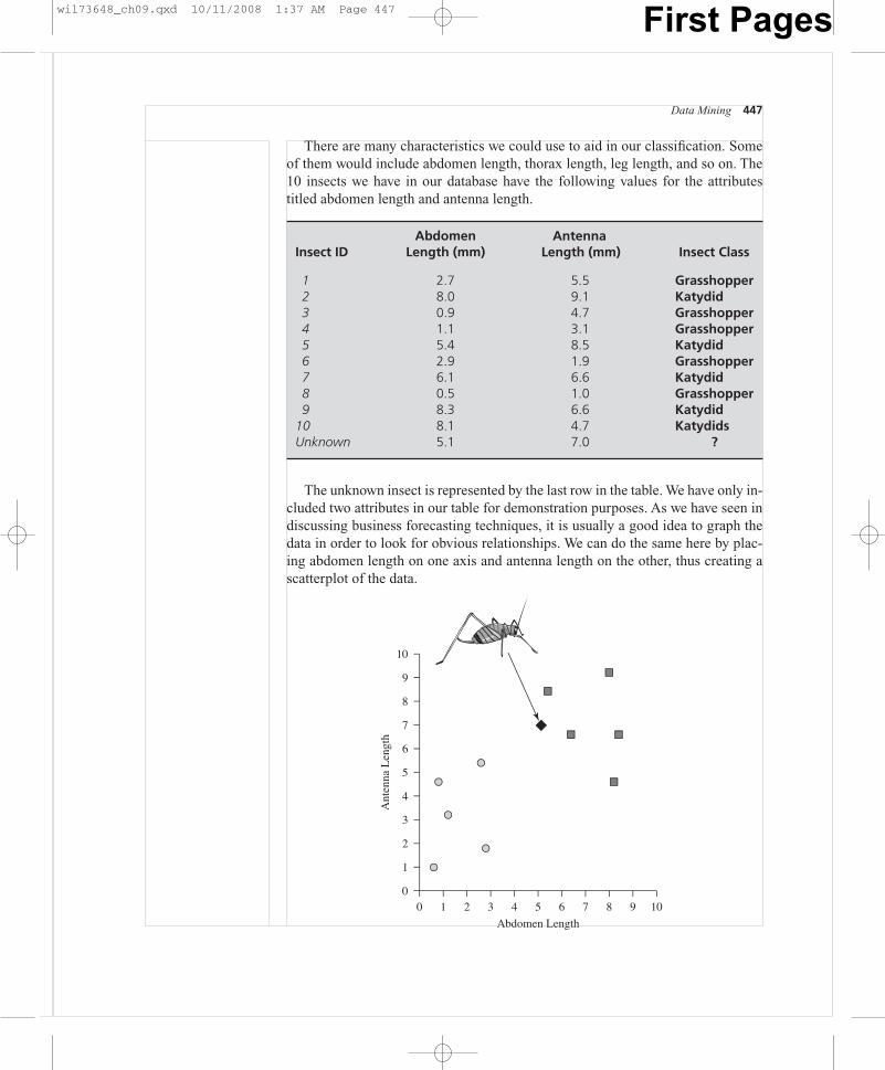
There are many characteristics we could use to aid in our classification. Someof them would include abdomen length, thorax length, leg length, and so on. The10 insects we have in our database have the following values for the attributestitled abdomen length and antenna length.

0

1

2

3

4

5

6

7

Ant

enna

Len

gth

8

9

10

4 5

Abdomen Length

106 7 8 90 1 2 3

The unknown insect is represented by the last row in the table. We have only in-cluded two attributes in our table for demonstration purposes. As we have seen indiscussing business forecasting techniques, it is usually a good idea to graph thedata in order to look for obvious relationships. We can do the same here by plac-ing abdomen length on one axis and antenna length on the other, thus creating ascatterplot of the data.


448 Chapter Nine

0

1

2

3

4

5

6

7

Ant

enna

Len

gth

8

9

10

4 5

Abdomen Length

106 7 8 90 1 2 3

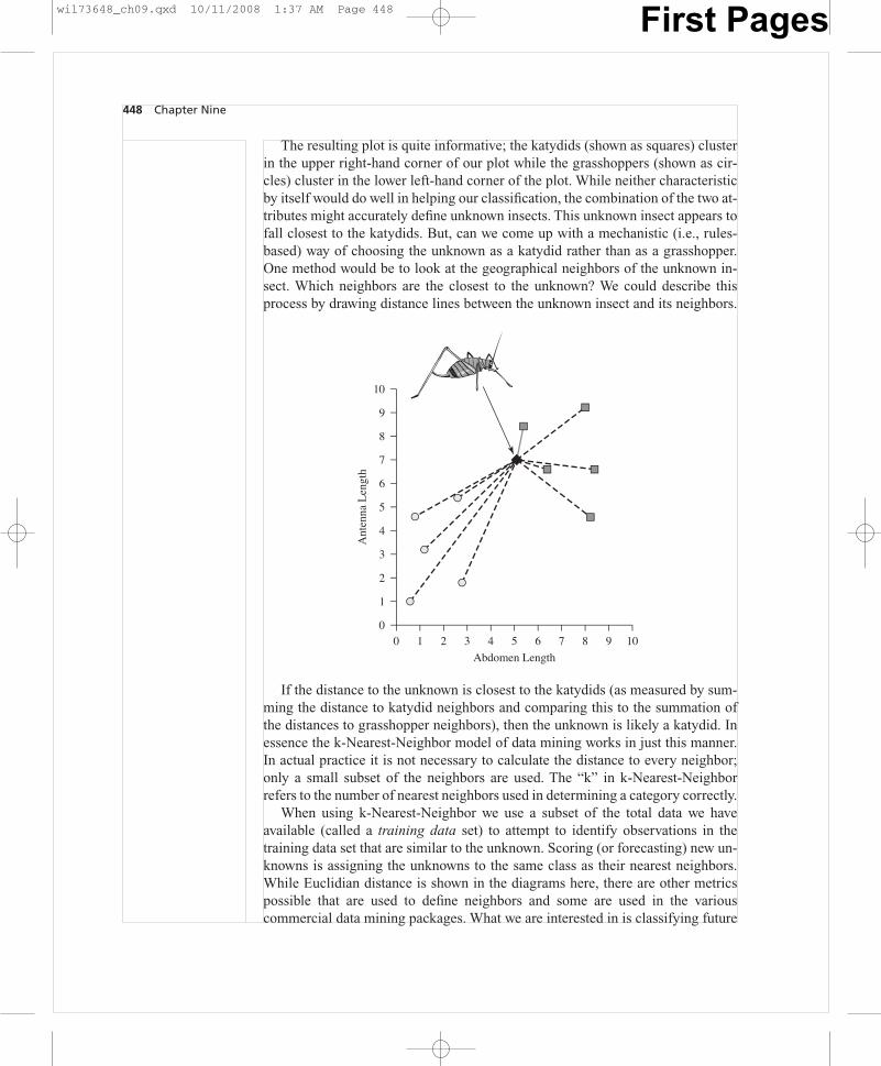
The resulting plot is quite informative; the katydids (shown as squares) clusterin the upper right-hand corner of our plot while the grasshoppers (shown as cir-cles) cluster in the lower left-hand corner of the plot. While neither characteristicby itself would do well in helping our classification, the combination of the two at-tributes might accurately define unknown insects. This unknown insect appears tofall closest to the katydids. But, can we come up with a mechanistic (i.e., rules-based) way of choosing the unknown as a katydid rather than as a grasshopper.One method would be to look at the geographical neighbors of the unknown in-sect. Which neighbors are the closest to the unknown? We could describe thisprocess by drawing distance lines between the unknown insect and its neighbors.

If the distance to the unknown is closest to the katydids (as measured by sum-ming the distance to katydid neighbors and comparing this to the summation ofthe distances to grasshopper neighbors), then the unknown is likely a katydid. Inessence the k-Nearest-Neighbor model of data mining works in just this manner.In actual practice it is not necessary to calculate the distance to every neighbor;only a small subset of the neighbors are used. The “k” in k-Nearest-Neighborrefers to the number of nearest neighbors used in determining a category correctly.

When using k-Nearest-Neighbor we use a subset of the total data we haveavailable (called a training data set) to attempt to identify observations in thetraining data set that are similar to the unknown. Scoring (or forecasting) new un-knowns is assigning the unknowns to the same class as their nearest neighbors.While Euclidian distance is shown in the diagrams here, there are other metricspossible that are used to define neighbors and some are used in the variouscommercial data mining packages. What we are interested in is classifying future


Cognos is a company providing data mining softwareto a variety of industries. One of those industries ishigher education. The University of North Texas hasmore than 33,000 students in 11 colleges that offer96 different bachelor’s degrees, 111 different mas-ter’s degrees and 50 different doctorate degrees. The

university uses data mining to identify student pref-erences and forecast what programs will attract cur-rent and future students. Admission, faculty hiring,and resource allocation are all affected by the out-comes of the data mining performed by EnterpriseInformation Systems at the university.

449

Comments from the Field Cognos 2

unknown insects, not the past performance on old data. We already know theclassifications of the insects in the training data set; that’s why we call it a trainingdata set. It trains the model to correctly classify the unknowns by selecting close-ness to the k-nearest-neighbors. So, the error rate on old data will not be veryuseful in determining if we have a good classification model. An error rate on atraining set is not the best indicator of future performance. To predict how wellthis model might do in the real world at classifying of unknowns we need to use itto classify some data that the model has not previously had access to; we need touse data that was not part of the training data set. This separate data set is calledthe validation data. In one sense, this separation of data into a training data set anda validation data set is much like the difference between “in-sample” test statisticsand “out-of-sample” test statistics. The real test of a business forecast was the “out-of-sample” test; the real test of a data mining model will be the test statistics onthe validation data, not the statistics calculated from the training data.

In order to produce reliable measures of the effectiveness of a data mining toolresearchers partition a data set before building a data mining model. It is standardpractice to divide the data set into partitions using some random procedure. Wecould, for instance, assign each instance in our data set a number and then parti-tion the data set into two parts called the training data and the validation data(sometimes researchers use a third partition called the test set). If there is a greatdeal of data (unlike the simple example of the katydids and grasshoppers), there islittle trouble in using 60 percent of the data as a training set and the remaining40 percent as a validation data set. This will insure that no effectiveness statisticsare drawn from the data used to create the model. Thus an early step in any realdata mining procedure is to partition the data. It is common practice to fold thevalidation data back into the training data and re-estimate the model if the modelshows up well in the validation data.

5 Galit Shmueli, Nitin Patel, and Peter Bruce, Data Mining for Business Intelligence, (John Wiley& Sons, 2007).

A BUSINESS DATA MINING EXAMPLE: k-NEAREST-NEIGHBOR

What would such a model look like in a business situation? We now turn to ex-amining a data set used by Shmueli, Patel, and Bruce.5 This data set represents in-formation on the customers a bank has in its data warehouse. These individuals


450 Chapter Nine

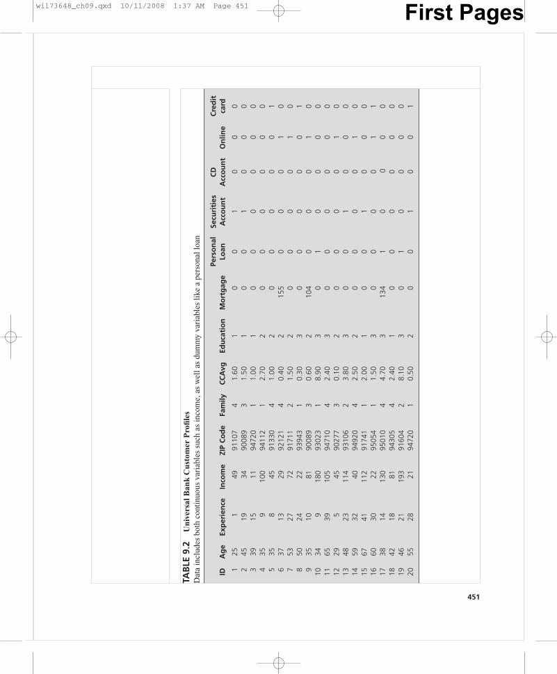
have been customers of the bank at some time in the past; perhaps many are cur-rent customers in one dimension or another. The type of information the bank hason each of these customers is represented in Tables 9.1 and 9.2.

Universal Bank would like to know which customers are likely to accept a per-sonal loan. What characteristics would forecast this? If the bank were to considerexpending advertising efforts to contact customers who would be likely to con-sider a personal loan, which customers should the bank contact first? By answer-ing this question correctly the bank will be able to optimize its advertising effortby directing its attention to the highest-yield customers.

This is a classification problem not unlike the situation of deciding in whatclass to place an unknown insect. The two classes in this example would be: (1)those with a high probability of accepting a personal loan (acceptors), and (2)those with a low probability of accepting a personal loan (nonacceptors). We willbe unable to classify customers with certainty about whether they will accept apersonal loan, but we may be able to classify the customers in our data into one ofthese two mutually exclusive categories.

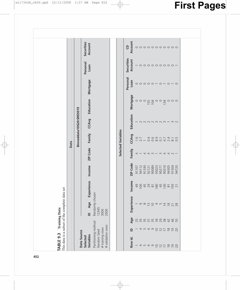
The researcher would begin by first partitioning the Universal Bank data. Re-call that partitioning the data set is the first step in any data mining technique.Since each row, or record, is a different customer we could assign a number toeach row and use a random selection process to choose 60 percent of the data as atraining set. All data mining software has such an option available. Once the datais selected into a training set it would look like Table 9.3. This table is producedusing the XLMiner© software.

ID Customer ID

Age Customer’s age in completed yearsExperience No. of years of professional experienceIncome Annual income of the customer ($000)ZIP code Home address, ZIP codeFamily Family size of the customerCC Avg. Average spending on credit cards per month ($000)Education Education level (1) Undergrad; (2) Graduate;

(3) Advanced/ProfessionalMortgage Value of house mortgage if any ($000)Personal loan Did this customer accept the personal loan offered in the

last campaign?Securities account Does the customer have a securities account with the

bank?CD account Does the customer have a certificate of deposit (CD)

account with the bank?Online Does the customer use Internet banking facilities?Credit card Does the customer use a credit card issued by Universal

Bank?

TABLE 9.1Universal Bank(Fictitious) Data The Bank Has Dataon a Customer-by-Customer Basis inthese Categories


451

TAB

LE 9

.2U

nive

rsal

Ban

k C

usto

mer

Pro

files

Dat

a in

clud

es b

oth

cont

inuo

us v

aria

bles

suc

h as

inco

me,

as

wel

l as

dum

my

vari

able

s li

ke a

per

sona

l loa

n

IDA

ge

Exp

erie

nce

Inco

me

ZIP

Co

de

Fam

ilyC

CA

vgEd

uca

tio

nM

ort

gag

ePe

rso

nal

Loan

125

149

9110

74

1.60

10

01

00

02

4519

3490

089

31.

501

00

10

00

339

1511

9472

01

1.00

10

00

00

04

359

100

9411

21

2.70

20

00

00

05

358

4591

330

41.

002

00

00

01

637

1329

9212

14

0.40

215

50

00

10

753

2772

9171

12

1.50

20

00

01

08

5024

2293

943

10.

303

00

00

01

935

1081

9008

93

0.60

210

40

00

10

1034

918

093

023

18.

903

01

00

00

1165

3910

594

710

42.

403

00

00

00

1229

545

9027

73

0.10

20

00

01

013

4823

114

9310

62

3.80

30

01

00

014

5932

4094

920

42.

502

00

00

10

1567

4111

291

741

12.

001

00

10

00

1660

3022

9505

41

1.50

30

00

01

117

3814

130

9501

04

4.70

313

41

00

00

1842

1881

9430

54

2.40

10

00

00

019

4621

193

9160

42

8.10

30

10

00

020

5528

2194

720

10.

502

00

10

01

Secu

riti

esA

cco

un

tC

DA

cco

un

tO

nlin

eC

red

itca

rd


452

TAB

LE 9

.3T

rain

ing

Dat

aT

his

data

is a

sub

set o

f th

e co

mpl

ete

data

set

Dat

a

Dat

a So

urc

eB

inn

edd

ata1

D$2

0:$R

$501

9

Sele

cted

Var

iab

les

IDA

ge

Exp

erie

nce

Inco

me

ZIP

Co

de

Fam

ilyC

CA

vgEd

uca

tio

nM

ort

gag

e

11

251

4991

107

41.

61

00

10

44

359

100

9411

21

2.7

20

00

05

535

845

9133

04

12

00

00

66

3713

2992

121

40.

42

155

00

09

935

1081

9008

93

0.6

210

40

00

1010

349

180

9302

31

8.9

30

10

012

1229

545

9027

73

0.1

20

00

017

1738

1413

095

010

44.

73

134

10

018

1842

1881

9430

54

2.4

10

00

019

1946

2119

391

504

28.

13

01

00

2020

5528

2194

720

10.

52

00

10

Pers

on

alLo

anSe

curi

ties

Acc

ou

nt

Part

ition

ing

met

hod

Rand

omly

cho

sen

Rand

om S

eed

1234

5#

trai

ning

row

s30

00#

valid

atio

n ro

ws

2000

Sele

cted

Var

iab

les

Ro

w Id

.ID

Ag

eEx

per

ien

ceIn

com

eZI

P C

od

eFa

mily

CC

Avg

Edu

cati

on

Mo

rtg

age

Pers

on

alLo

anSe

curi

ties

Acc

ou

nt

CD

Acc

ou

nt


Note that the “Row ID” in Table 9.3 skips from row 1 to row 5 and then fromrow 6 to row 9. This is because the random selection process has chosen cus-tomers 1, 4, 5, 6, and 9 for the training data set (displayed in Table 9.3) but hasplaced customers 2, 3, 7, and 8 in the validation data set (not displayed in Table9.3). Examining the header to Table 9.3 you will note that there were a total of5,000 customers in the original data set that have now been divided into a trainingdata set of 3,000 customers and a validation data set of 2,000 customers.

When we instruct the software to perform a k-Nearest-Neighbor analysis ofthe training data the real data mining analysis takes place. Just as in the insectclassification example, the software will compare each customer’s personal loanexperience with the selected attributes. This example is, of course, much moremultidimensional since we have many attributes for each customer (as opposed toonly the two attributes we used in the insect example). The program will computethe distance associated with each attribute. For attributes that are measured ascontinuous variables, the software will normalize the distance and then measure it(because different continuous attributes are measured in different scales). For thedummy type or categorical attributes, most programs use a weighting mechanismthat is beyond the scope of this treatment.

The accuracy measures for the estimated model will tell if we have possiblyfound a useful classification scheme. In this instance we want to find a way toclassify customers as likely to accept a personal loan. How accurately can we dothat by considering the range of customer attributes in our data? Are there some at-tributes that could lead us to classify some customers as much more likely to accepta loan and other customers as quite unlikely?While the accuracy measures are oftenproduced by the software for both the training data set and the validation data set,our emphasis should clearly be on those measures pertaining to the validation data.There are two standard accuracy measures we will examine: the classificationmatrix (also called the confusion matrix) and the lift chart.The classification matrixfor the Universal Bank data training data is shown in Table 9.4.

When our task is classification, accuracy is often measured in terms of errorrate, the percentage of records we have classified incorrectly. The error rate isoften displayed for both the training data set and the validation data set in separatetables. Table 9.4 is such a table for the validation data set in the Universal Bank

Data Mining 453

Validation Data Scoring—Summary Report (for k � 3)

Cut off prob. val. for success (updatable) 0.5

Classification Confusion Matrix

Predicted Class

Actual Class 1 0

1 118 760 8 1798

TABLE 9.4Classification Matrix(confusion matrix)for the UniversalBank DataThe number of nearestneighbors we havechosen is 3.


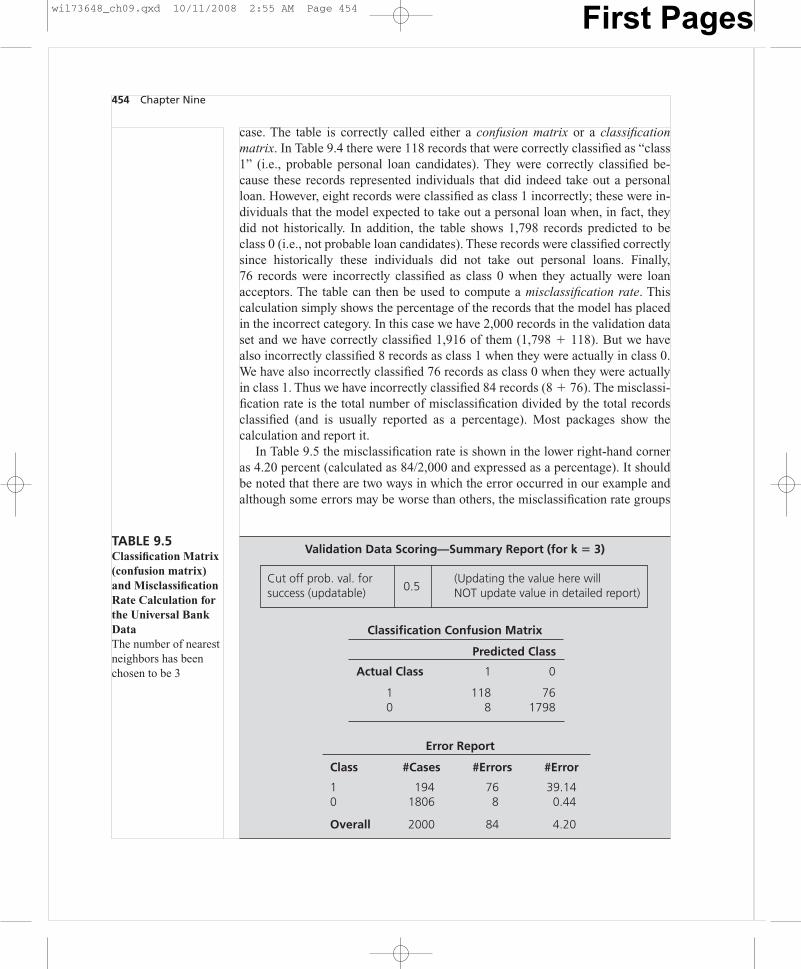
case. The table is correctly called either a confusion matrix or a classificationmatrix. In Table 9.4 there were 118 records that were correctly classified as “class1” (i.e., probable personal loan candidates). They were correctly classified be-cause these records represented individuals that did indeed take out a personalloan. However, eight records were classified as class 1 incorrectly; these were in-dividuals that the model expected to take out a personal loan when, in fact, theydid not historically. In addition, the table shows 1,798 records predicted to beclass 0 (i.e., not probable loan candidates). These records were classified correctlysince historically these individuals did not take out personal loans. Finally,76 records were incorrectly classified as class 0 when they actually were loanacceptors. The table can then be used to compute a misclassification rate. Thiscalculation simply shows the percentage of the records that the model has placedin the incorrect category. In this case we have 2,000 records in the validation dataset and we have correctly classified 1,916 of them (1,798 � 118). But we havealso incorrectly classified 8 records as class 1 when they were actually in class 0.We have also incorrectly classified 76 records as class 0 when they were actuallyin class 1. Thus we have incorrectly classified 84 records (8 � 76). The misclassi-fication rate is the total number of misclassification divided by the total recordsclassified (and is usually reported as a percentage). Most packages show thecalculation and report it.

In Table 9.5 the misclassification rate is shown in the lower right-hand corneras 4.20 percent (calculated as 84/2,000 and expressed as a percentage). It shouldbe noted that there are two ways in which the error occurred in our example andalthough some errors may be worse than others, the misclassification rate groups

454 Chapter Nine

Validation Data Scoring—Summary Report (for k � 3)

Cut off prob. val. forsuccess (updatable) 0.5

(Updating the value here willNOT update value in detailed report)


Predicted Class

Actual Class 1 0

1 118 760 8 1798

Error Report

Class #Cases #Errors #Error

1 194 76 39.140 1806 8 0.44

Overall 2000 84 4.20

TABLE 9.5Classification Matrix(confusion matrix)and MisclassificationRate Calculation forthe Universal BankDataThe number of nearestneighbors has beenchosen to be 3


Data Mining 455

Validation Error Log for Different k

Value of k % Error Training % Error Validation

1 0.00 5.302 1.30 5.303 2.70 4.20 <— Best k4 2.80 4.205 3.43 4.706 3.27 4.507 3.70 4.858 3.40 4.309 4.47 5.15

10 4.00 4.8511 4.83 5.6512 4.33 5.3513 5.00 5.6014 4.60 5.3515 5.20 5.7016 4.93 5.4017 5.33 5.7518 5.23 5.6019 5.83 6.0020 5.60 5.90

TABLE 9.6Validation Error Log for the UniversalBank DataThe best number ofnearest neighborshas been chosen tobe 3 because thisprovides the lowestmisclassification rate

these two types of errors together. While this may not be an ideal reporting mech-anism, it is commonly used and displayed by data mining software. Some soft-ware also allows placing different costs on the different types of errors as a way ofdifferentiating their impacts. While the overall error rate of 4.2 percent in the val-idation data is low in this example, the error of classifying an actual loan acceptorincorrectly as a non-loan acceptor (76 cases) is much greater than that of incor-rectly classifying an actual nonacceptor as a loan acceptor (only 8 cases).

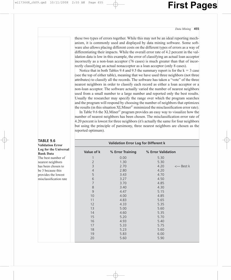
Notice that in both Tables 9.4 and 9.5 the summary report is for the k � 3 case(see the top of either table), meaning that we have used three neighbors (not threeattributes) to classify all the records. The software has taken a “vote” of the threenearest neighbors in order to classify each record as either a loan acceptor or anon-loan acceptor. The software actually varied the number of nearest neighborsused from a small number to a large number and reported only the best results.Usually the researcher may specify the range over which the program searchesand the program will respond by choosing the number of neighbors that optimizesthe results (in this situation XLMiner© minimized the misclassification error rate).

In Table 9.6 the XLMiner© program provides an easy way to visualize how thenumber of nearest neighbors has been chosen. The misclassification error rate of4.20 percent is lowest for three neighbors (it’s actually the same for four neighborsbut using the principle of parsimony, three nearest neighbors are chosen as thereported optimum).


456 Chapter Nine

FIGURE 9.1 Lift Chart and Decile-wise Lift Chart for the Universal Bank ValidationData Set

00 1000 2000

# cases

3000

50

100

150

Cum

ulat

ive

200

250

Cumulative personal loan whensorted using predicted values

Cumulative personal loanusing average

Lift Chart (Validation Dataset)

01 2 3 4 5 6 7 8 9 10

Deciles

4

3

2

1

5

6

Dec

ile M

ean/

Glo

bal M

ean

7

8Decile-wise Lift Chart (Validation Dataset)

Lift

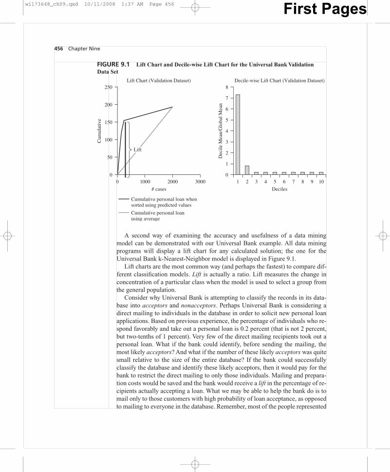
A second way of examining the accuracy and usefulness of a data miningmodel can be demonstrated with our Universal Bank example. All data miningprograms will display a lift chart for any calculated solution; the one for theUniversal Bank k-Nearest-Neighbor model is displayed in Figure 9.1.

Lift charts are the most common way (and perhaps the fastest) to compare dif-ferent classification models. Lift is actually a ratio. Lift measures the change inconcentration of a particular class when the model is used to select a group fromthe general population.

Consider why Universal Bank is attempting to classify the records in its data-base into acceptors and nonacceptors. Perhaps Universal Bank is considering adirect mailing to individuals in the database in order to solicit new personal loanapplications. Based on previous experience, the percentage of individuals who re-spond favorably and take out a personal loan is 0.2 percent (that is not 2 percent,but two-tenths of 1 percent). Very few of the direct mailing recipients took out apersonal loan. What if the bank could identify, before sending the mailing, themost likely acceptors? And what if the number of these likely acceptors was quitesmall relative to the size of the entire database? If the bank could successfullyclassify the database and identify these likely acceptors, then it would pay for thebank to restrict the direct mailing to only those individuals. Mailing and prepara-tion costs would be saved and the bank would receive a lift in the percentage of re-cipients actually accepting a loan. What we may be able to help the bank do is tomail only to those customers with high probability of loan acceptance, as opposedto mailing to everyone in the database. Remember, most of the people represented


in the database are not likely loan acceptors. Only a relatively small number of therecords in the database represent acceptors.

The lift curve is drawn from information about what the k-Nearest Neighbormodel predicted in a particular case and what that individual actually did. The liftchart in Figure 9.1 is actually a cumulative gains chart. It is constructed with therecords arranged on the x-axis left to right from the highest probability to lowestprobability of accepting a loan. The y-axis reports the number of true positives atevery point (i.e., the y-axis counts the number of records that represent actual loanacceptors).

Looking at the decile-wise lift chart in Figure 9.1 we can see that if we were tochoose the top 10 percent of the records classified by our model (i.e., the 10 per-cent most likely to accept a personal loan) our selection would include approxi-mately seven times as many correct classifications than if we were to select a ran-dom 10 percent of the database. That’s a dramatic lift provided by the model whencompared to a random selection.

The same information is displayed in a different manner in the lift chart on theleft-hand side of Figure 9.1. This lift chart represents the cumulative records cor-rectly classified (on the y-axis), with the records arranged in descending probabil-ity order on the x-axis. Since the curve inclines steeply upward over the first fewhundred cases displayed on the x-axis, the model appears to provide significant liftrelative to a random selection of records. Generally a better model will displayhigher lift than other candidate models. Lift can be used to compare the perform-ance of models of different kinds (e.g., k-Nearest Neighbor models comparedwith other data mining techniques and is a good tool for comparing the perform-ance of two or more data mining models using the same or comparable data. No-tice the straight line rising at a 45-degree angle in the lift chart in Figure 9.1—thisis a reference line. The line represents how well you might do by classifying as aresult of random selection. If the calculated lift line is significantly above this ref-erence line, you may expect the model to outperform a random selection. In theUniversal Bank case the k-Nearest Neighbor model outperforms a random selec-tion by a very large margin.

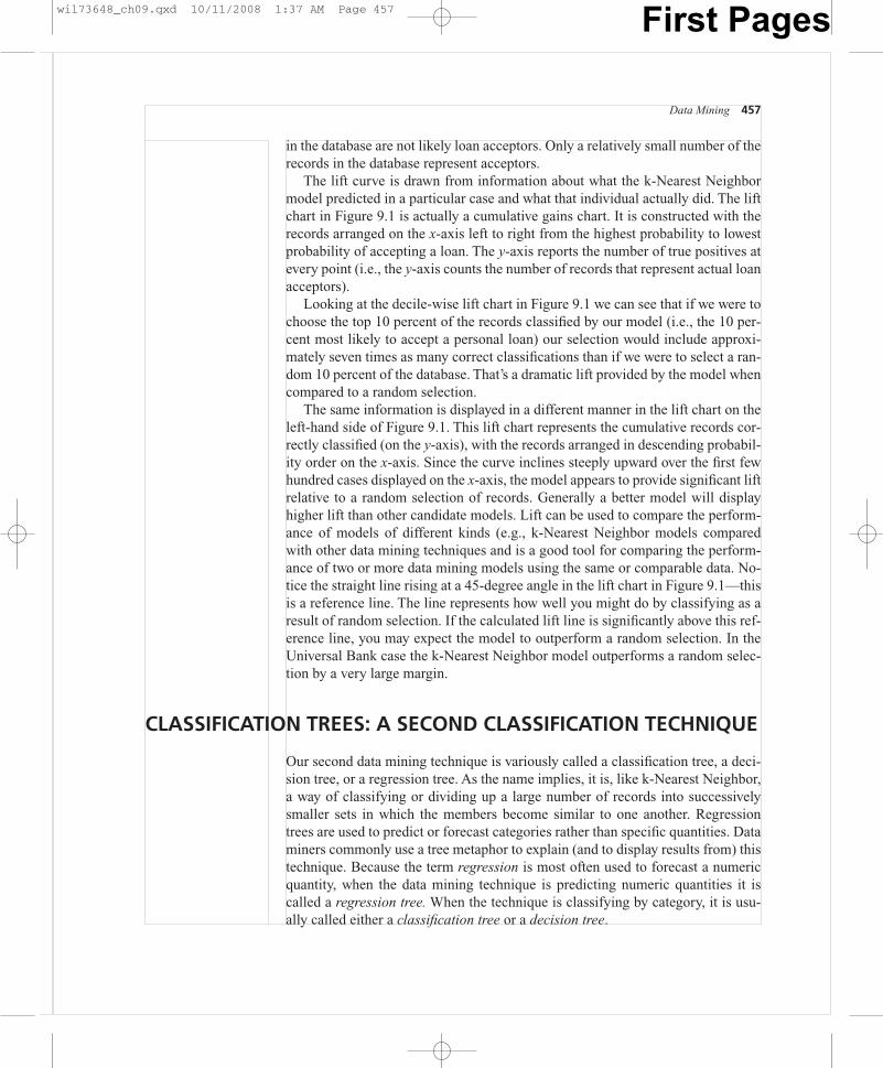
CLASSIFICATION TREES: A SECOND CLASSIFICATION TECHNIQUE

Our second data mining technique is variously called a classification tree, a deci-sion tree, or a regression tree. As the name implies, it is, like k-Nearest Neighbor,a way of classifying or dividing up a large number of records into successivelysmaller sets in which the members become similar to one another. Regressiontrees are used to predict or forecast categories rather than specific quantities. Dataminers commonly use a tree metaphor to explain (and to display results from) thistechnique. Because the term regression is most often used to forecast a numericquantity, when the data mining technique is predicting numeric quantities it iscalled a regression tree. When the technique is classifying by category, it is usu-ally called either a classification tree or a decision tree.

Data Mining 457


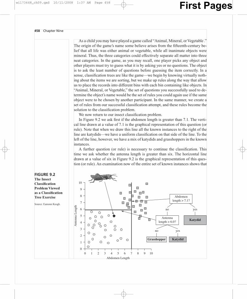
As a child you may have played a game called “Animal, Mineral, or Vegetable .”The origin of the game’s name some believe arises from the fifteenth-century be-lief that all life was either animal or vegetable, while all inanimate objects weremineral. Thus, the three categories could effectively separate all matter into threeneat categories. In the game, as you may recall, one player picks any object andother players must try to guess what it is by asking yes or no questions. The objectis to ask the least number of questions before guessing the item correctly. In asense, classification trees are like the game—we begin by knowing virtually noth-ing about the items we are sorting, but we make up rules along the way that allowus to place the records into different bins with each bin containing like objects. In“Animal, Mineral, or Vegetable,” the set of questions you successfully used to de-termine the object’s name would be the set of rules you could again use if the sameobject were to be chosen by another participant. In the same manner, we create aset of rules from our successful classification attempt, and these rules become thesolution to the classification problem.

We now return to our insect classification problem.In Figure 9.2 we ask first if the abdomen length is greater than 7.1. The verti-

cal line drawn at a value of 7.1 is the graphical representation of this question (orrule). Note that when we draw this line all the known instances to the right of theline are katydids—we have a uniform classification on that side of the line. To theleft of the line, however, we have a mix of katydids and grasshoppers in the knowninstances.

A further question (or rule) is necessary to continue the classification. Thistime we ask whether the antenna length is greater than six. The horizontal linedrawn at a value of six in Figure 9.2 is the graphical representation of this ques-tion (or rule). An examination now of the entire set of known instances shows that

458 Chapter Nine

FIGURE 9.2The InsectClassificationProblem Viewed as a ClassificationTree Exercise


0

1

2

3

4

5

6

7

Ant

enna

Len

gth

8

9

10

4 5

Abdomen Length

106 7 8 90 1 2 3

Abdomenlength > 7.1?

Antennalength > 6.0?

no yes

no yes

KatydidGrasshopper

Katydid


there is homogeneity in each region defined by our two questions. The right-handregion contains only katydids as does the topmost region in the upper left-handcorner. The bottommost region in the lower left-hand corner, however, containsonly grasshoppers. Thus we have divided the geometric attribute space into threeregions, each containing only a single type of insect.

In asking the two questions to create the three regions, we have also created therules necessary to perform further classifications on unknown insects. Take theunknown insect shown in the diagram with an antenna length of 5 and an abdomenlength of 4.5. By asking whether the unknown has an abdomen length of greaterthan 7.1 (answer � no) and then asking whether the antenna length is greater than6 (answer � no), the insect is correctly classified as a grasshopper.

In our example we have used only two attributes (abdomen length and antennalength) to complete the classification routine. In a real world situation we need notconfine ourselves to only two attributes. In fact, we can use many attributes. Thegeometric picture might be difficult to draw but the decision tree (shown on theright-hand side of Figure 9.2) would look much the same as it does in our simpleexample. In data mining terminology, the two decision points in Figure 9.2 (shownas “abdomen length � 7.1” and “antenna length � 6”) are called decision nodes.Nodes in XLMiner© are shown as circles with the decision value shown inside.They are called decision nodes because we classify unknowns by “dropping”them through the tree structure in much the same way a ball drops throughPachinko game. (See Figure 9.3).

The bottom of our classification tree in Figure 9.2 has three leaves. Each leaf isa terminal node in the classification process; it represents the situation in which allthe instances that follow that branch result in uniformity. The three leaves inFigure 9.2 are represented by the shaded boxes at the bottom of the diagram. Datamining classification trees are upside-down in that the leaves are at the bottomwhile the root of the tree is at the top; this is the convention in data mining circles.To begin a scoring process all the instances are at the root (i.e., top) of the tree;these instances are partitioned by the rules we have determined with the knowninstances. The result is that the unknown instances move downward through thetree until reaching a leaf node at which point they are (hopefully) successfullyclassified.

At times the classification trees can become quite large and ungainly. It iscommon for data mining programs to prune the trees to remove branches. The un-pruned tree was made using the training data set and it probably matches that dataperfectly. Does that mean that this unpruned tree will do the best job in classify-ing new unknown instances? Probably not. A good classification tree algorithmwill make the best split (at the first decision node) first followed by decision rulesthat are made up with successively smaller and smaller numbers of trainingrecords. These later decision rules will become more and more idiosyncratic. Theresult may be an unstable tree that will not do well in classifying new instances.Thus the need for pruning. Each data mining package uses a proprietary pruningalgorithm that usually takes into account for any branch the added drop in the mis-classification rate versus the added tree complexity. XLMiner© and other data

Data Mining 459


mining programs use candidate tree formulations with the validation data set tofind the lowest validation data set misclassification rate—that tree is selected asthe final best-pruned tree. While the actual process is more complicated thanwe have described here, our explanation is essentially correct for all data miningsoftware.

Classification trees are very popular in actual practice because the decisionrules are easily generated and, more importantly, because the trees themselves areeasy to understand and explain to others. There are disadvantages as well however.The classification trees can suffer from overfitting and if are not pruned well, thesetrees may not result in good classifications of new data (i.e., they will not scorenew data well). Attributes that are correlated will also cause this technique seriousproblems. It is somewhat similar to multicollinearity in a regression model. Becareful not to use features that are very closely correlated one with another.

460 Chapter Nine

FIGURE 9.3Classic PachinkoGameA ball falls from thetop through to thebottom and is guidedby an array of pins.The user normallycontrols only thespeed at which theball enters the playingfield. Like a slotmachine the gameis usually played inhope of winning apayoff.


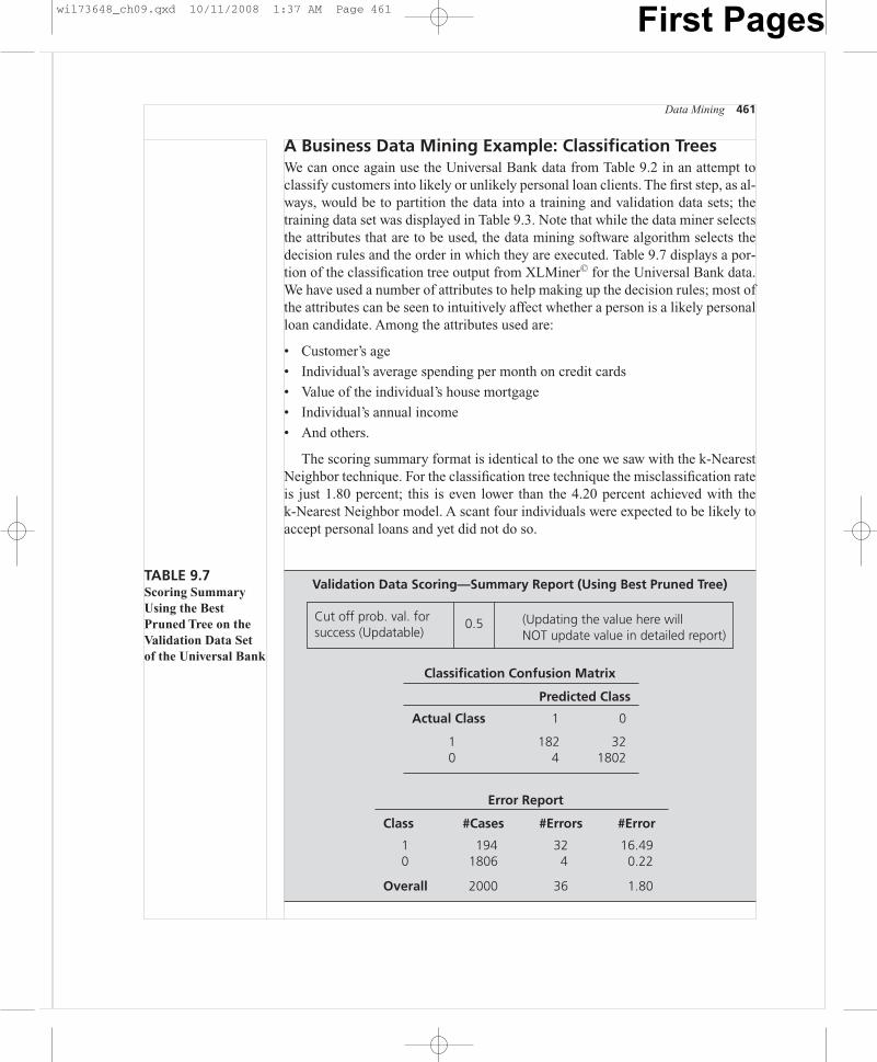
A Business Data Mining Example: Classification TreesWe can once again use the Universal Bank data from Table 9.2 in an attempt toclassify customers into likely or unlikely personal loan clients. The first step, as al-ways, would be to partition the data into a training and validation data sets; thetraining data set was displayed in Table 9.3. Note that while the data miner selectsthe attributes that are to be used, the data mining software algorithm selects thedecision rules and the order in which they are executed. Table 9.7 displays a por-tion of the classification tree output from XLMiner© for the Universal Bank data.We have used a number of attributes to help making up the decision rules; most ofthe attributes can be seen to intuitively affect whether a person is a likely personalloan candidate. Among the attributes used are:

• Customer’s age

• Individual’s average spending per month on credit cards

• Value of the individual’s house mortgage

• Individual’s annual income

• And others.

The scoring summary format is identical to the one we saw with the k-NearestNeighbor technique. For the classification tree technique the misclassification rateis just 1.80 percent; this is even lower than the 4.20 percent achieved with thek-Nearest Neighbor model. A scant four individuals were expected to be likely toaccept personal loans and yet did not do so.

Data Mining 461

Validation Data Scoring—Summary Report (Using Best Pruned Tree)

Cut off prob. val. for success (Updatable)

0.5 (Updating the value here willNOT update value in detailed report)


Predicted Class

Actual Class 1 0

1 182 320 4 1802

Error Report

Class #Cases #Errors #Error

1 194 32 16.490 1806 4 0.22

Overall 2000 36 1.80

TABLE 9.7Scoring SummaryUsing the BestPruned Tree on theValidation Data Setof the Universal Bank


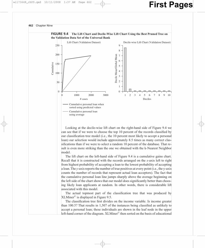
Looking at the decile-wise lift chart on the right-hand side of Figure 9.4 wecan see that if we were to choose the top 10 percent of the records classified byour classification tree model (i.e., the 10 percent most likely to accept a personalloan) our selection would include approximately 8.5 times as many correct clas-sifications than if we were to select a random 10 percent of the database. That re-sult is even more striking than the one we obtained with the k-Nearest Neighbormodel.

The lift chart on the left-hand side of Figure 9.4 is a cumulative gains chart.Recall that it is constructed with the records arranged on the x-axis left to rightfrom highest probability of accepting a loan to the lowest probability of acceptinga loan. The y-axis reports the number of true positives at every point (i.e., the y-axiscounts the number of records that represent actual loan acceptors). The fact thatthe cumulative personal loan line jumps sharply above the average beginning onthe left side of the chart shows that our model does significantly better than choos-ing likely loan applicants at random. In other words, there is considerable liftassociated with this model.

The actual topmost part of the classification tree that was produced byXLMiner© is displayed in Figure 9.5.

The classification tree first divides on the income variable. Is income greaterthan 100.5? That results in 1,507 of the instances being classified as unlikely toaccept a personal loan; these individuals are shown in the leaf node in the upperleft-hand corner of the diagram. XLMiner© then sorted on the basis of educational

462 Chapter Nine

FIGURE 9.4 The Lift Chart and Decile-Wise Lift Chart Using the Best Pruned Tree onthe Validation Data Set of the Universal Bank

00 1000 2000

# cases

3000

50

100

150

Cum

ulat

ive

200

250




01 2 3 4 5 6 7 8 9 10

Deciles

4

3

2

1

5

6

Dec

ile M

ean/

Glo

bal M

ean

8

7



level followed by sorts based upon the family size of the customer (Family) andthe annual income of the customer (Income). While examining the tree in Fig-ure 9.5 is useful, it may be more instructive to examine the rules that are exempli-fied by the tree. Some of those rules are displayed in Table 9.8.

The rules displayed in Table 9.8 represent the same information shown in thediagram in Figure 9.5. Examining the first row of the table shows the split value as100.5 for the split variable of income. This is the same as asking if the individualhad a yearly income greater than 100.5? It is called a decision node because thereare two branches extending downward from this node (i.e., it is not a terminalnode or leaf). The second row of the table contains the information shown in theleaf on the left-hand side of the classification tree in Figure 9.5; this is called aterminal node or leaf because there are no successors. Row two shows that

Data Mining 463

FIGURE 9.5The Topmost Portionof the ClassificationTree Using the BestPruned Tree on theValidation Data Setof the Universal Bank

100.5

Income493

Education

1507

1.5

177316

116.5

IncomeFamily

56 121276 40

2.5

0

TABLE 9.8 The Topmost Portion of the Tree Rules Using the Best Pruned Tree on the Validation Data Setof the Universal Bank

Best Pruned Tree Rules (Using Validation Data)

#Decision nodes 8 #Terminal nodes 9

Level Node ID Parent ID Split Var Split Value Cases Left Child Right Child Class Node Type

0 0 N/A Income 100.5 2000 1 2 0 Decision1 1 0 N/A N/A 1507 N/A N/A 0 Terminal1 2 0 Education 1.5 493 3 4 0 Decision2 3 2 Family 2.5 316 5 6 0 Decision


1,507 cases are classified at 0, or unlikely to take out a personal loan in thisterminal node. It is these rules displayed in this table that the program uses toscore new data, and they provide a concise and exact way to treat new data in aspeedy manner.

If actual values are predicted (as opposed to categories) for each case, then thetree is called a regression tree. For instance, we could attempt to predict the sell-ing price of a used car by examining a number of attributes of the car. The relevantattributes might include the age of the car, the mileage the car had been driven todate, the original selling price of the car when new, and so on. The predictionwould be expected to be an actual number, not simply a category. The process wehave described could, however, still be used in this case. The result would be a setof rules that would determine the predicted price.

NAIVE BAYES: A THIRD CLASSIFICATION TECHNIQUE

A third and somewhat different approach to classification uses statistical classi-fiers. This technique will predict the probability that an instance is a member of acertain class. This technique is based on Bayes’ theorem; we will describe the the-orem below. In actual practice these Naive Bayes algorithms have been found tobe comparable in performance to the decision trees we examined above. One hall-mark of the Naive Bayes model is speed, along with high accuracy. This model iscalled naive because it assumes (perhaps naively) that each of the attributes is in-dependent of the values of the other attributes. Of course this will never be strictlytrue, but in actual practice the assumption (although somewhat incorrect) allowsthe rapid determination of a classification scheme and does not seem to suffer ap-preciably in accuracy when such an assumption is made.

To explain the basic procedure we return to our insect classification example.Our diagram may be of the same data we have used before, but we will examine itin a slightly different manner.

The known instances of katydids and grasshoppers are again shown in Fig-ure 9.6, but only a single attribute of interest is labeled on the y-axis: antennalength. On the right-hand side of Figure 9.6 we have drawn a histogram of the an-tenna lengths for grasshoppers and a separate histogram representing the antennalength of katydids.

Now assume we wish to use this information about a single attribute to classifyan unknown insect. Our unknown insect has a measured antenna length of 3 (asshown in Figure 9.7). Look on the problem as an entirely statistical problem. Isthis unknown more likely to be in the katydid distribution or the grasshopper dis-tribution? A length of 3 would be in the far right tail of the katydid distribution(and therefore unlikely to be a part of that distribution). But a length of 3 issquarely in the center of the grasshopper distribution (and therefore it is morelikely to be a member of that distribution). Of course there is the possibility thatthe unknown with an antenna length of 3 is actually part of the katydid distribu-

464 Chapter Nine


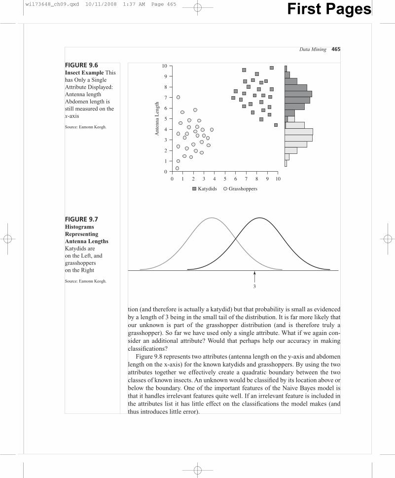
tion (and therefore is actually a katydid) but that probability is small as evidencedby a length of 3 being in the small tail of the distribution. It is far more likely thatour unknown is part of the grasshopper distribution (and is therefore truly agrasshopper). So far we have used only a single attribute. What if we again con-sider an additional attribute? Would that perhaps help our accuracy in makingclassifications?

Figure 9.8 represents two attributes (antenna length on the y-axis and abdomenlength on the x-axis) for the known katydids and grasshoppers. By using the twoattributes together we effectively create a quadratic boundary between the twoclasses of known insects. An unknown would be classified by its location above orbelow the boundary. One of the important features of the Naive Bayes model isthat it handles irrelevant features quite well. If an irrelevant feature is included inthe attributes list it has little effect on the classifications the model makes (andthus introduces little error).

Data Mining 465

FIGURE 9.6Insect Example Thishas Only a SingleAttribute Displayed:Antenna lengthAbdomen length isstill measured on thex-axis


0

1

2

3

4

5

6

7

Ant

enna

Len

gth

8

9

10

4 5 106 7 8 90 1 2 3

Katydids Grasshoppers

FIGURE 9.7HistogramsRepresentingAntenna LengthsKatydids areon the Left, andgrasshoppers on the Right

Source: Eamonn Keogh.3


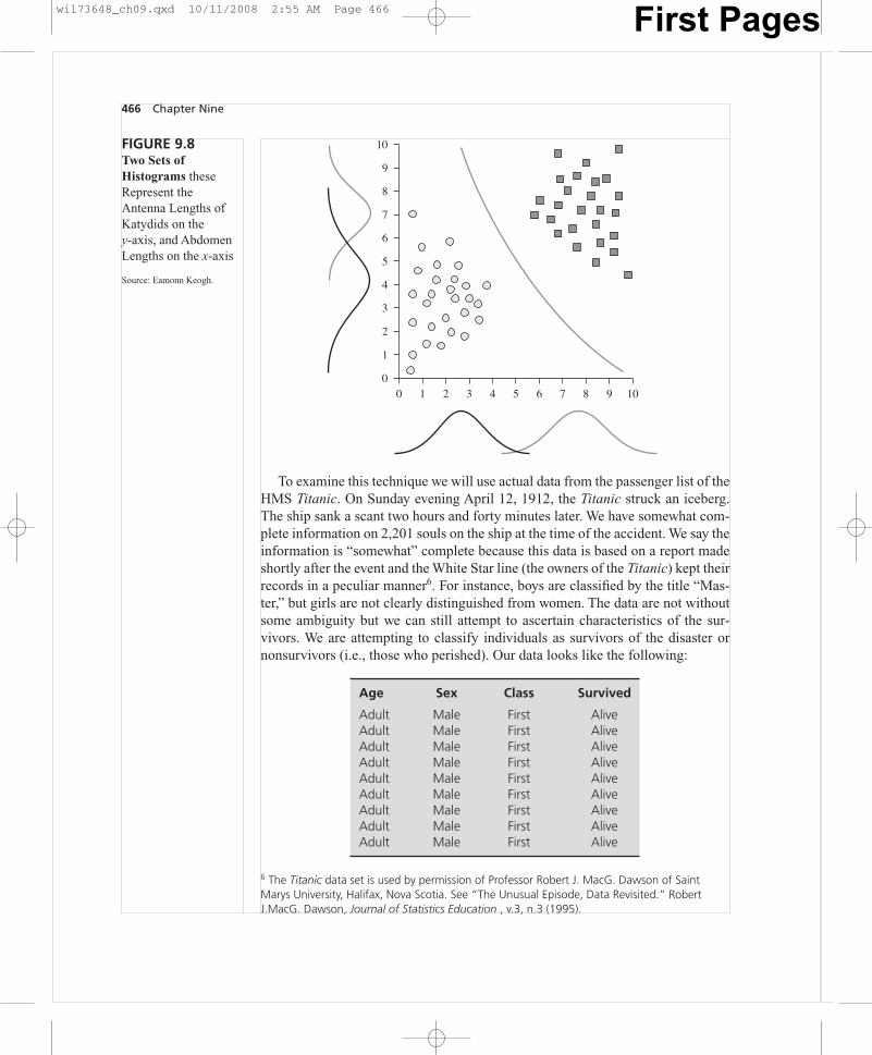
To examine this technique we will use actual data from the passenger list of theHMS Titanic. On Sunday evening April 12, 1912, the Titanic struck an iceberg.The ship sank a scant two hours and forty minutes later. We have somewhat com-plete information on 2,201 souls on the ship at the time of the accident. We say theinformation is “somewhat” complete because this data is based on a report madeshortly after the event and the White Star line (the owners of the Titanic) kept theirrecords in a peculiar manner6. For instance, boys are classified by the title “Mas-ter,” but girls are not clearly distinguished from women. The data are not withoutsome ambiguity but we can still attempt to ascertain characteristics of the sur-vivors. We are attempting to classify individuals as survivors of the disaster ornonsurvivors (i.e., those who perished). Our data looks like the following:

Age Sex Class Survived

Adult Male First AliveAdult Male First AliveAdult Male First AliveAdult Male First AliveAdult Male First AliveAdult Male First AliveAdult Male First AliveAdult Male First AliveAdult Male First Alive

466 Chapter Nine

FIGURE 9.8Two Sets ofHistograms theseRepresent theAntenna Lengths ofKatydids on they-axis, and AbdomenLengths on the x-axis


0

1

2

3

4

5

6

7

8

9

10

4 5 106 7 8 90 1 2 3

6 The Titanic data set is used by permission of Professor Robert J. MacG. Dawson of SaintMarys University, Halifax, Nova Scotia. See “The Unusual Episode, Data Revisited.” RobertJ.MacG. Dawson, Journal of Statistics Education , v.3, n.3 (1995).


The data set contains information on each of the individuals on the Titanic. Weknow whether they were adult or child, whether they were male or female, theclass of their accommodations (first class passenger, second class, third class, orcrew), and whether they survived that fateful night. In our list 711 are listed asalive while 1,490 listed as dead; thus only 32 percent of the people on boardsurvived.

What if we wished to examine the probability that an individual with certaincharacteristics (say, an adult, male crew member) were to survive? Could we usethe Naive Bayes method to determine the probability that this person survived?The answer is Yes; that is precisely what a Naive Bayes model will do. In this casewe are classifying the adult, male crew member into one of two categories: sur-vivor or dead.

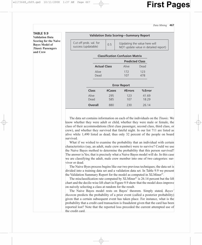
The Naive Byes process begins like our two previous techniques; the data set isdivided into a training data set and a validation data set. In Table 9.9 we presentthe Validation Summary Report for the model as computed in XLMiner©.

The misclassification rate computed by XLMiner© is 26.14 percent but the liftchart and the decile-wise lift chart in Figure 9.9 show that the model does improveon naively selecting a class at random for the result.

The Naive Bayes model rests on Bayes’ theorem. Simply stated, Bayes’theorem predicts the probability of a prior event (called a posterior probability)given that a certain subsequent event has taken place. For instance, what is theprobability that a credit card transaction is fraudulent given that the card has beenreported lost? Note that the reported loss preceded the current attempted use ofthe credit card.

Data Mining 467

Validation Data Scoring—Summary Report

Cut off prob. val. forsuccess (updatable)



Predicted Class

Actual Class Alive Dead

Alive 172 123Dead 107 478

Error Report

Class #Cases #Errors %Error

Alive 295 123 41.69Dead 585 107 18.29

Overall 880 230 26.14

TABLE 9.9Validation Data Scoring for the NaiveBayes Model ofTitanic Passengersand Crew


The posterior probability is written as P(A | B ). Thus , P(A | B ) is the proba-bility that the credit card use is fraudulent given that we know the card has beenreported lost. P(A ) would be called the prior probability of A and is the probabil-ity that any credit card transaction is fraudulent regardless of whether the card isreported lost.

The Bayesian theorem is stated in the following manner:

P(A | B) � �P(B | A)

��P(B)

P(A)�

where:

P(A) is the prior probability of A. It is prior in the sense that it does not takeinto account any information about B.

P(A | B) is the conditional probability of A, given B. It is also called theposterior probability because it is derived from or depends upon the specifiedvalue of B. This is the probability we are usually seeking to determine.

P(B | A) is the conditional probability of B given A.

P(B) is the prior probability of B.

An example will perhaps make the use of Bayes’ theorem clearer. Consider thatwe have the following data set showing eight credit card transactions. For eachtransaction we have information about whether the transaction was fraudulent andwhether the card used was previously reported lost (see Table 9.10).

468 Chapter Nine

FIGURE 9.9 Lift Chart and Decile-Wise Lift Chart for the Naive Bayes Titanic Model

00 500

# cases

1000

50

100

150

Cum

ulat

ive

200

300

250

350

Cumulative survived whensorted using predicted values

Cumulative survived usingaverage


01 2 3 4 5 6 7 8 9 10

Deciles

2

1.5

1

0.5

2.5

Dec

ile M

ean/

Glo

bal M

ean



Data Mining 469

Applying Bayes’ theorem:

P(Fraud | Card Reported Lost) � �P(Lost

��| Fraud )

P(Lost)��

P(Fraud )�

��23��

38�

� _________ � .667�38

and

P(NonFraud | Card Reported Lost) � �P(Lost

��| No

�nFraud )

P(Lost)��

P(Non�Fraud )

�

��15��

58�

� _________ � .333�38

Thus, the probability of a fraudulent transaction if the card has been reportedlost is 66.7 percent. The probability of a nonfraudulent transaction if the card hasbeen reported lost is 33.3 percent.

Returning to the Titanic data and the Naive Bayes model calculated byXLMiner©, we may now demonstrate the calculation of the posterior probabili-ties of interest. These are the answers to our question concerning the probabil-ity that an adult, male crew member would survive the disaster. XLMiner© pro-duces an additional output for the Naive Bayes model displaying the prior classprobabilities and the calculated conditional probabilities. These are displayed inTable 9.11.

To answer our question concerning the survival probability of an adult, malecrew member we need once again to apply Bayes’ theorem. We first need to cal-culate the conditional probabilities required in the Bayes’ theorem:

Conditional probability of “alive”if you were a crew member, male, and adult:

P(alive) � (0.295673077)(.53125)(.9375)(0.314912945) � 0.046373782

Transaction No. Fraudulent? Reported Lost?

1 Yes Yes2 No No3 No No4 No No5 Yes Yes6 No No7 No Yes8 Yes No

TABLE 9.10Credit CardTransaction Data Set


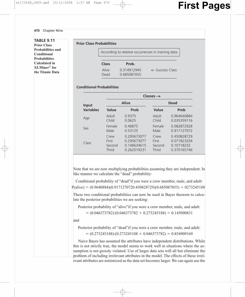
Note that we are now multiplying probabilities assuming they are independent. Inlike manner we calculate the “dead” probability:

Conditional probability of “dead”if you were a crew member, male, and adult:

P(alive) � (0.9640884)(0.9171270720.450828729)(0.685087055) � 0273245188

These two conditional probabilities can now be used in Bayes theorem to calcu-late the posterior probabilities we are seeking:

Posterior probability of “alive”if you were a crew member, male, and adult:

� (0.046373782)/(0.046373782 � 0.273245188) � 0.145090831

and

Posterior probability of “dead”if you were a crew member, male, and adult:

� (0.273245188)/(0.273245188 � 0.046373782) � 0.854909169

Naive Bayes has assumed the attributes have independent distributions. Whilethis is not strictly true, the model seems to work well in situations where the as-sumption is not grossly violated. Use of larger data sets will all but eliminate theproblem of including irrelevant attributes in the model. The effects of these irrel-evant attributes are minimized as the data set becomes larger. We can again use the

470 Chapter Nine

Classes —>

InputAlive Dead

Variables Value Prob Value Prob

Age Adult 0.9375 Adult 0.964640884Child 0.0625 Child 0.035359116

Sex Female 0.46875 Female 0.082872928Male 0.53125 Male 0.917127072

Crew 0.295673077 Crew 0.450828729

Class First 0.295673077 First 0.071823204Second 0.146634615 Second 0.10718232Third 0.262019231 Third 0.370165746

TABLE 9.11Prior ClassProbabilities andConditionalProbabilitiesCalculated inXLMiner© for the Titanic Data

Prior Class Probabilities

According to relative occurrences in training data

Class Prob.

Alive 0.314912945 <— Success ClassDead 0.685087055

Conditional Probabilities


Universal Bank data and apply the Naive Bayes model in order to predict cus-tomers that will accept a personal loan. Figure 9.10 displays the Naive Bayes re-sults from XLMiner© for the Universal Bank data.

Once again it is clear that the model performs much better than a naive selec-tion of individuals when we try to select possible loan acceptors. Looking at thedecile-wise lift chart on the right-hand side of Figure 9.10 we can see that if we

Data Mining 471





Predicted Class

Actual Class 1 0

1 122 720 77 1729

Error Report


1 194 72 37.110 1806 77 4.26

Overall 2000 149 7.45

FIGURE 9.10The Naive BayesModel Applied tothe Universal BankDataIncluded are confusion matrix, misclassificationrate, and lift charts

00 1000 2000

# cases

3000

50

100

150

Cum

ulat

ive

200

250




01 2 3 4 5 6 7 8 9 10

Deciles

4

3

2

1

5

6

Dec

ile M

ean/

Glo

bal M

ean



were to choose the top 10 percent of the records classified by our classificationtree model (i.e., the 10 percent most likely to accept a personal loan) our selectionwould include approximately 6.5 times as many correct classifications than if wewere to select a random 10 percent of the database. While Naive Bayes models doextremely well on training data, in real world applications these models tend notto do quite as well as other classification models in some situations. This is likelydue to the disregard of the model for attribute interdependence. In many realworld situations, however, Naive Bayes models do just as well as other classifica-tion models. While the Naive Bayes model is relatively simple, it makes sense totry the simplest models first and to use them if they provide sufficient results.Clearly data sets that contain highly interdependent attributes will fare poorlywith Naive Bayes.

REGRESSION: A FOURTH CLASSIFICATION TECHNIQUE

Our final classification data mining technique is logistic regression or logit analy-sis (both names refer to the same method). This technique is a natural complementto linear least squares regression. It has much in common with ordinary linear re-gression models we examined in Chapters 4 and 5. Ordinary linear regressionprovides a universal framework for much of economic analysis; its simplifiedmanner of looking at data has proven useful to researchers and forecasters fordecades. Logistic regression serves the same purpose for categorical data. Thesingle most important distinction between logistic regression and ordinary regres-sion is that the dependent variable in logistic regression is categorical (and notcontinuous). The explanatory variables, or attributes, may be either continuous orcategorical (as they were in linear least squares models). Just like the ordinary lin-ear regression model, logistic regression is able to use all sorts of extensions andsophisticated variants. Logistic regression has found its way into the toolkits ofnot only forecasters and economists; also, for example, into those of toxicologistsand epidemiologists.

TRUE LIFTVictor S. Y. Lo of Fidelity Investments uses logisticregression models and Naive Bayes models to dif-ferentiate between customers who would be ex-pected to respond to some sort of stimulus (e.g., amail campaign or a telephone call) from customerswho would respond without any added stimulus.He calls the result true lift. The methods Lo usespecifically find customers who will take a desir-able action regardless of the treatment. His aim

was to find the characteristics of customers whoseresponse decisions can be positively influenced by acampaign. Customer development campaigns, in-cluding upselling and cross-selling, would benefitgreatly from such a tool.

Source: Victor S. Y. Lo, “The True Lift Model—A NovelData Mining Approach to Response Modeling inDatabase Marketing,” SIGKDD Explorations, December2002, Volume 4, Issue 2, p. 74–86.

Comments from the Field 3

472


Data Mining 473

The Universal Bank situation we have been examining provides a case in point.The dependent variable, the item we are attempting to forecast, is dichotomous—either a person accepts a loan or rejects the loan. There is no continuous variablehere; it is more like an on/off switch. But why are we unable to use linear leastsquares models on this data?

Consider Table 9.12—it contains information about 20 students, the hours theyspent studying for a qualifying exam, and their results. If they passed the exam thetable shows a 1, if they failed the exam, the table shows a 0.

If we graph this data as a scatterplot we see there are two possible outcomes:pass (shown as 1) and fail (shown as 0).

Student No. Hours of Study Pass/Fail

1 2.5 02 22.6 13 17.8 04 5.4 05 14 06 13.3 17 26 18 33.1 19 13.6 0

10 45.3 111 1.9 012 31.4 113 27 114 10.1 015 2.7 016 16.3 117 14.5 118 4.5 019 22.6 120 17.1 1

TABLE 9.12Data on 20 Studentsand Their TestPerformance andHours of Study.

FIGURE 9.11Scatterplot ofStudent Performance

00

0.2

0.4

0.6

0.8

1

1.2Pass/Fail

Pass/Fail

10 20 30 40 50


474 Chapter Nine

It appears from the scatterplot that students who spent more time studying forthe exam had a better chance of passing. We might seek to quantify this percep-tion by running a least squares regression using “hours of study” as the independ-ent variable and “pass/fail” as the dependent variable. Running this regression re-sults in the output in Table 9.13.

Since the “hours of study” coefficient is positive (�0.03), it appears to indicatethat more study leads to a higher probability of passing. But, is the relationshipcorrectly quantified? Suppose an individual studies for 100 hours. How well willthis individual do on the exam? Substituting into the regression equation we have:

Pass/fail � 0.002053 � (0.032072) � (100)

3.209253 � 0.002053 � (0.032072) � (100)

What does this mean? Is the predicted grade 3.209 percent? This doesn’t seemto make sense. Examining the regression line estimated and superimposing it onthe data scatter may make the problem clear (see Figure 9.12).

The difficulty becomes clearer when examining the diagram. There are only twostates of nature for the dependent variable (pass and fail). However, the regressionline plotted in Figure 9.12 is a straight line sloping upward to the right and predict-ing values all along its path. When predicting the outcome from 100 hours of studythe regression chooses a number (i.e., 3.209253) that is much greater than the max-imum value of 1 exhibited in the data set. Does this mean the individual has passedthe test 3.209 times? Or does this mean that the expected score is 3.209 percent? Ordoes this have any meaningful explanation at all? This result means that we haveused an inappropriate tool in attempting to find the answer to our question. In ear-lier chapters we assumed the dependent variable was continuous, this one is not.Linear least squares regression does not restrict the predictions of the dependentvariable to a range of zero to one as we would like in this case.

We would really like to use this same data but predict the probability that an in-dividual would pass the test given a certain number of hours of study. We willmodify the linear least squares model by modifying what we use as the dependentvariable. Ordinarily we simply use Y as the dependent variable; in logistic regres-sion we will use a function of Y as the dependent variable instead. This function ofthe dependent variable will be limited to values between zero and one. The func-tion we use is called a logit and that is the reason the technique is called logisticregression.

Audit Trail--Coefficient Table (Multiple Regression Selected)

Series

Description

TABLE 9.13 Linear Least Squares Regression

Included

in Model Coefficient

Standard

Error T-test P-value Elasticity

Overall

F-test---------------------------------------------------------------------------------------Hours of Study Yes 0.03 0.01 4.47 0.00 1.00

Pass/Fail Dependent 0.0020532033 0.15 0.01 0.99 20.02


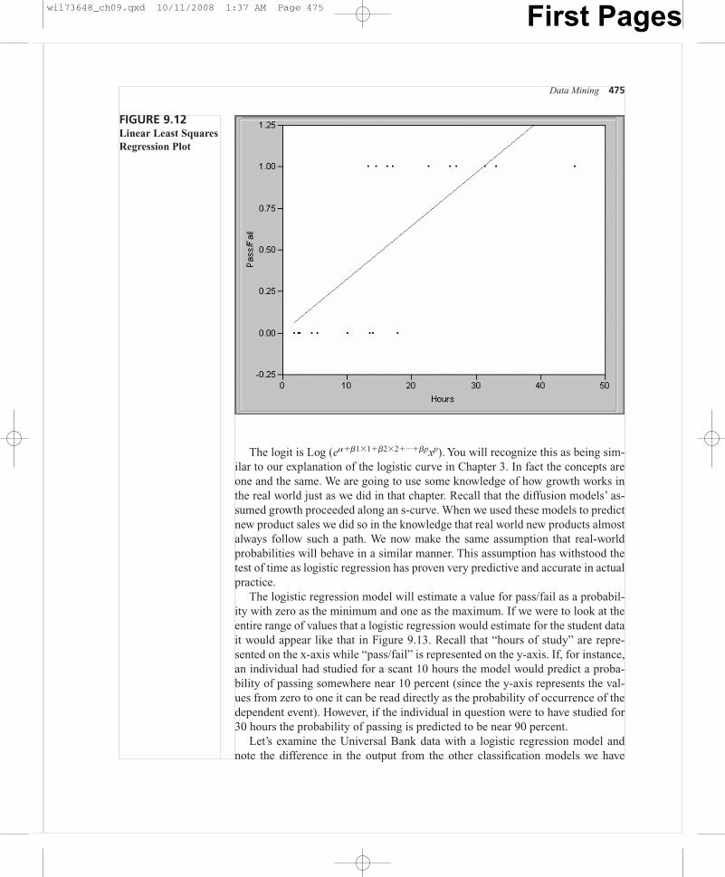
Data Mining 475

FIGURE 9.12Linear Least SquaresRegression Plot

The logit is Log (e��1�1��2�2�...��pxp). You will recognize this as being sim-ilar to our explanation of the logistic curve in Chapter 3. In fact the concepts areone and the same. We are going to use some knowledge of how growth works inthe real world just as we did in that chapter. Recall that the diffusion models’ as-sumed growth proceeded along an s-curve. When we used these models to predictnew product sales we did so in the knowledge that real world new products almostalways follow such a path. We now make the same assumption that real-worldprobabilities will behave in a similar manner. This assumption has withstood thetest of time as logistic regression has proven very predictive and accurate in actualpractice.

The logistic regression model will estimate a value for pass/fail as a probabil-ity with zero as the minimum and one as the maximum. If we were to look at theentire range of values that a logistic regression would estimate for the student datait would appear like that in Figure 9.13. Recall that “hours of study” are repre-sented on the x-axis while “pass/fail” is represented on the y-axis. If, for instance,an individual had studied for a scant 10 hours the model would predict a proba-bility of passing somewhere near 10 percent (since the y-axis represents the val-ues from zero to one it can be read directly as the probability of occurrence of thedependent event). However, if the individual in question were to have studied for30 hours the probability of passing is predicted to be near 90 percent.

Let’s examine the Universal Bank data with a logistic regression model andnote the difference in the output from the other classification models we have


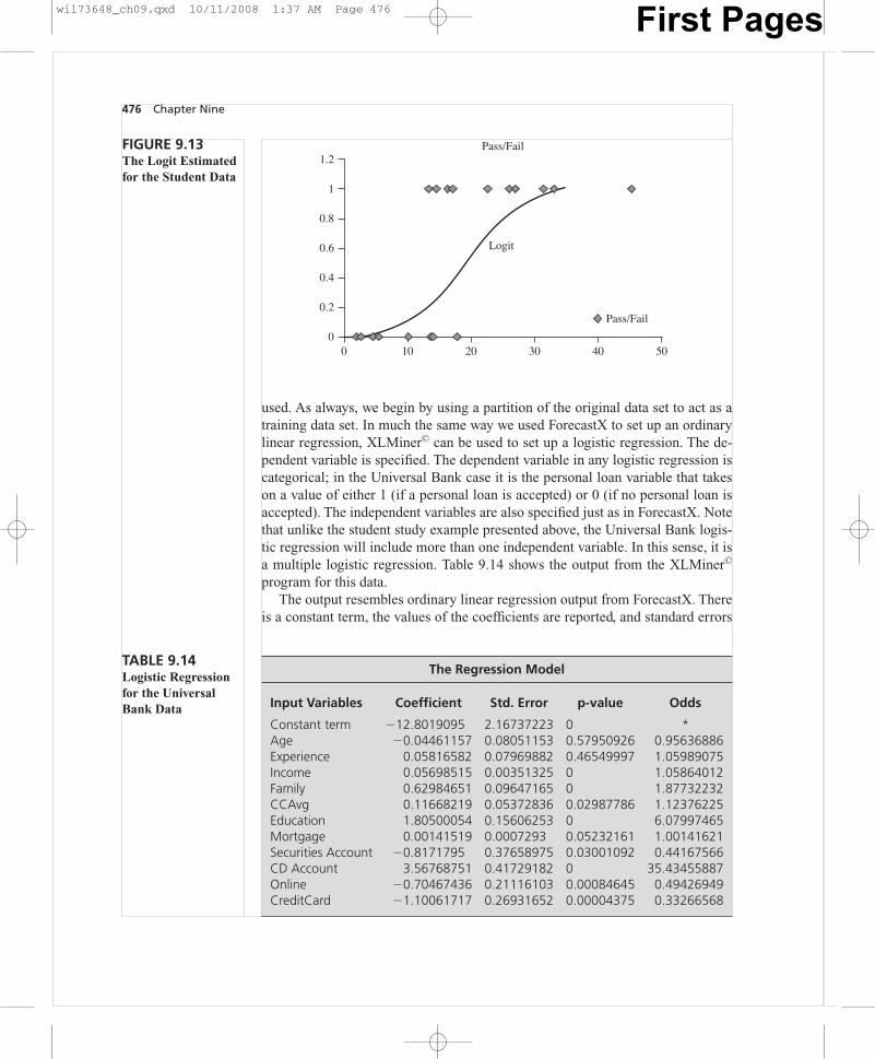
476 Chapter Nine

FIGURE 9.13The Logit Estimatedfor the Student Data

00

0.2

0.4

0.6

0.8

1

1.2Pass/Fail

Pass/Fail

Logit

10 20 30 40 50

used. As always, we begin by using a partition of the original data set to act as atraining data set. In much the same way we used ForecastX to set up an ordinarylinear regression, XLMiner© can be used to set up a logistic regression. The de-pendent variable is specified. The dependent variable in any logistic regression iscategorical; in the Universal Bank case it is the personal loan variable that takeson a value of either 1 (if a personal loan is accepted) or 0 (if no personal loan isaccepted). The independent variables are also specified just as in ForecastX. Notethat unlike the student study example presented above, the Universal Bank logis-tic regression will include more than one independent variable. In this sense, it isa multiple logistic regression. Table 9.14 shows the output from the XLMiner©

program for this data.The output resembles ordinary linear regression output from ForecastX. There

is a constant term, the values of the coefficients are reported, and standard errors

The Regression Model

Input Variables Coefficient Std. Error p-value Odds

Constant term �12.8019095 2.16737223 0 *Age �0.04461157 0.08051153 0.57950926 0.95636886Experience 0.05816582 0.07969882 0.46549997 1.05989075Income 0.05698515 0.00351325 0 1.05864012Family 0.62984651 0.09647165 0 1.87732232CCAvg 0.11668219 0.05372836 0.02987786 1.12376225Education 1.80500054 0.15606253 0 6.07997465Mortgage 0.00141519 0.0007293 0.05232161 1.00141621Securities Account �0.8171795 0.37658975 0.03001092 0.44167566CD Account 3.56768751 0.41729182 0 35.43455887Online �0.70467436 0.21116103 0.00084645 0.49426949CreditCard �1.10061717 0.26931652 0.00004375 0.33266568

TABLE 9.14Logistic Regressionfor the UniversalBank Data


for those coefficients allow p-values to be reported. The interpretation of thesevariables is much the same as it was with ordinary linear regression.

For example, the Family variable represents the family size of the customer.Since the logistic regression coefficient for this variable is positive (i.e.,+0.62984651) we would expect that the probability of accepting a personal loanincreases with family size. Further, since the p-value for this variable is very small(reported as zero in the printout but actually a very small number) we believe thatthe coefficient is significant at the 99 percent level. That is, we believe that thereis very little chance that the real relationship between family size and the accept-ance of a personal loan is zero. This ability to examine individual attributes is sim-ilar to the manner in which we examined the individual coefficients of an ordinarylinear regression.

Table 9.15 displays the validation data set confusion matrix and misclassifica-tion rate. This information allows us to judge in part the overall fit of the logisticregression model. The confusion matrix and misclassification rate give an overallsense of fit. In this case the 5.05 percent misclassification rate would indicate howwell we believe the model would classify new data into the correct categories.

The validation data set lift charts are also used to judge the overall fit of themodel. Examining the right-hand side of Figure 9.14 shows that selecting the top10 percent of the training data observations (i.e., those persons judged most likelyto accept a personal loan), resulted in a better that 7 times result when comparedto selecting individual cases at random. The same information is again displayedin the left-hand side of Figure 9.14 in the lift chart. The steep rise in the lift com-pared to the reference line for a naive selection of cases (i.e., the straight line inthe figure) shows significant explanatory power in the model.

Data Mining 477





Predicted Class

Actual Class 1 0

1 125 690 32 1774

Error Report


1 194 69 35.570 1806 32 1.77

Overall 2000 101 5.05

TABLE 9.15Logistic RegressionConfusion Matrixand MisclassificationRate


00 1000 2000

# cases

3000

50

100

150

Cum

ulat

ive

200

250




01 2 3 4 5 6 7 8 9 10

Deciles

4

3

2

1

5

6

7

Dec

ile M

ean/

Glo

bal M

ean


FIGURE 9.14 Validation Data Lift Charts for the Logistic Regression Model

BusinessWeek related the story of Michael Drosnin,author of a bestselling book, The Bible Code. In thebook Drosnin claimed to have found references inthe Bible to President Bill Clinton, dinosaurs andthe Land of Magog. Peter Coy, the author of thearticle, pointed out many of the useful tasks towhich data mining had been put (e.g., weedingout credit card fraud, finding sales prospects, anddiscovering new drugs).

But Coy also pointed out that data mining wasthe method used by Michael Drosnin to make his“discoveries” in the Bible. It seems Drosnin wroteout the Hebrew Bible as a grid of letters and useddata mining to look for words on the diagonal, up,down, and across. Not surprisingly he found somerecognizable words and references. Cryptic mes-sages appeared according to Coy such as the closejuxtaposition of the word dinosaur with the wordasteroid. According to Andrew Lo of the Massachu-setts Institute of Technology, ‘’Given enough time,enough attempts, and enough imagination, almostany pattern can be teased out of any data set.’’

The moral to the story is that a formula that fitsthe data may not have any predictive power at all!

There is always the chance that what a data miningtechnique “observes” or “discovers” may just be acoincidence in the current data set and not some-thing that is reproducible in the future with otherdata. The chance of this being true in data miningis more prominent than in the standard businessforecasting routines we presented earlier in thetext. Most of those techniques relied on proveneconomic theory as a basis for specifying a partic-ular type of model. With data mining it is the dataitself that specifies the model and the analystshould be wary of making the same mistake asMichael Drosnin. Coy gives the example of David J.Leinweber, managing director of First QuadrantCorporation who sifted through a United NationsCD-ROM and discovered that historically, the singlebest predictor of the Standard & Poor’s 500-stockindex was butter production in Bangladesh.Leinweber called this an example of “stupid dataminers’ tricks.”

Source: Peter Coy, “Commentary: He Who Mines DataMay Strike Fool’s Gold.” BusinessWeek , June 16, 1997,p. 40.

Comments from the Field: Fool’s Gold 4

478


Data Mining 479

SuggestedReadings

Berry, Michael J. A.; and Gordon S. Linhoff. Data Mining Techniques for Marketing, Sales,and Customer Relationship Management. Indianapolis: Wiley Publishing, Inc., 2004.

Cramer, J.S. Logit Models from Economics and Other Fields. Cambridge: CambridgeUniversity Press, 2003.

Han, Jiawei; and Micheline Kamber. Data Mining Concepts and Techniques. San Diego,California: Academic Press, 2001.

Shmueli, Galit; Nitin R. Patel; and Peter C. Bruce. Data Mining for Business Intelligence.Hoboken, New Jersey: John Wiley & Sons, Inc., 2007

Witten, Ian H.; and Eibe Frank. Data Mining: Practical Machine Learning Tools andTechniques. Amsterdam: Elsevier, 2005.

Exercises 1. A data mining routine has been applied to a transaction dataset and has classified 88records as fraudulent (30 correctly so) and 952 as nonfraudulent (920 correctly so).

The decile-wise lift chart for a transaction data model:

Interpret the meaning of the bars in this chart.

0

1

2

3

4

5

6

7

4 5

Deciles

Dec

ile M

ean/

Glo

bal M

ean

Decile-wise Lift Chart (Validation Dataset)

106 7 8 91 2 3

Summary In this chapter we have covered four classification techniques that are commonly used byreal data miners. Classification, however, is only a single aspect of data mining. In generalthere is no one best classification technique; the individual data in a particular situation willdetermine the best technique to use. The diagnostic statistics will lead the researcher tochoose an appropriate model; there may be no optimal model.

Data mining also uses other tools such as clustering analysis and neural network analy-sis. These tools are not covered here but there are excellent resources for those interested inpursuing the study of data mining. The growth in the use of commercial data mining toolsrivals the growth in business forecasting software sales; SAS Enterprise Miner and SPSSClementine have become important additions to the forecaster’s toolkit in recent years.


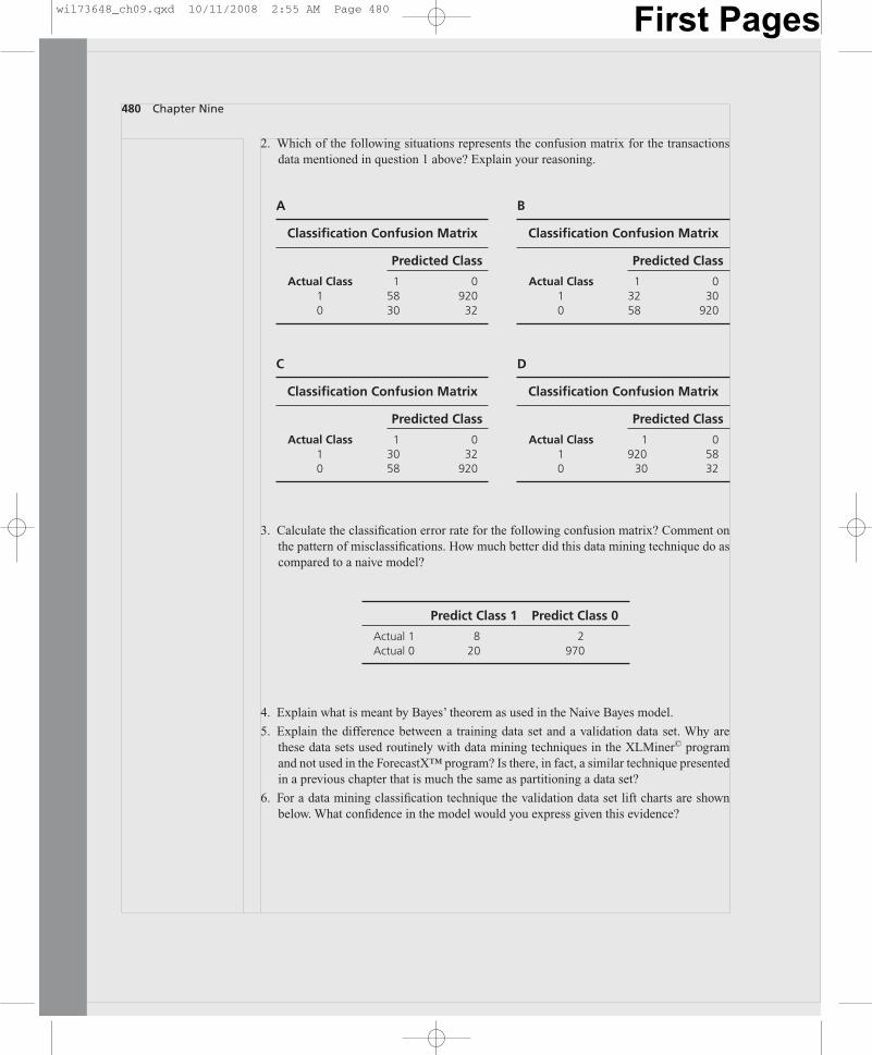
3. Calculate the classification error rate for the following confusion matrix? Comment onthe pattern of misclassifications. How much better did this data mining technique do ascompared to a naive model?

480 Chapter Nine

Predict Class 1 Predict Class 0

Actual 1 8 2Actual 0 20 970

4. Explain what is meant by Bayes’ theorem as used in the Naive Bayes model.

5. Explain the difference between a training data set and a validation data set. Why arethese data sets used routinely with data mining techniques in the XLMiner© programand not used in the ForecastX™ program? Is there, in fact, a similar technique presentedin a previous chapter that is much the same as partitioning a data set?

6. For a data mining classification technique the validation data set lift charts are shownbelow. What confidence in the model would you express given this evidence?

C


Predicted Class

Actual Class 1 01 30 320 58 920

D


Predicted Class

Actual Class 1 01 920 580 30 32

A


Predicted Class

Actual Class 1 01 58 9200 30 32

B


Predicted Class

Actual Class 1 01 32 300 58 920

2. Which of the following situations represents the confusion matrix for the transactionsdata mentioned in question 1 above? Explain your reasoning.


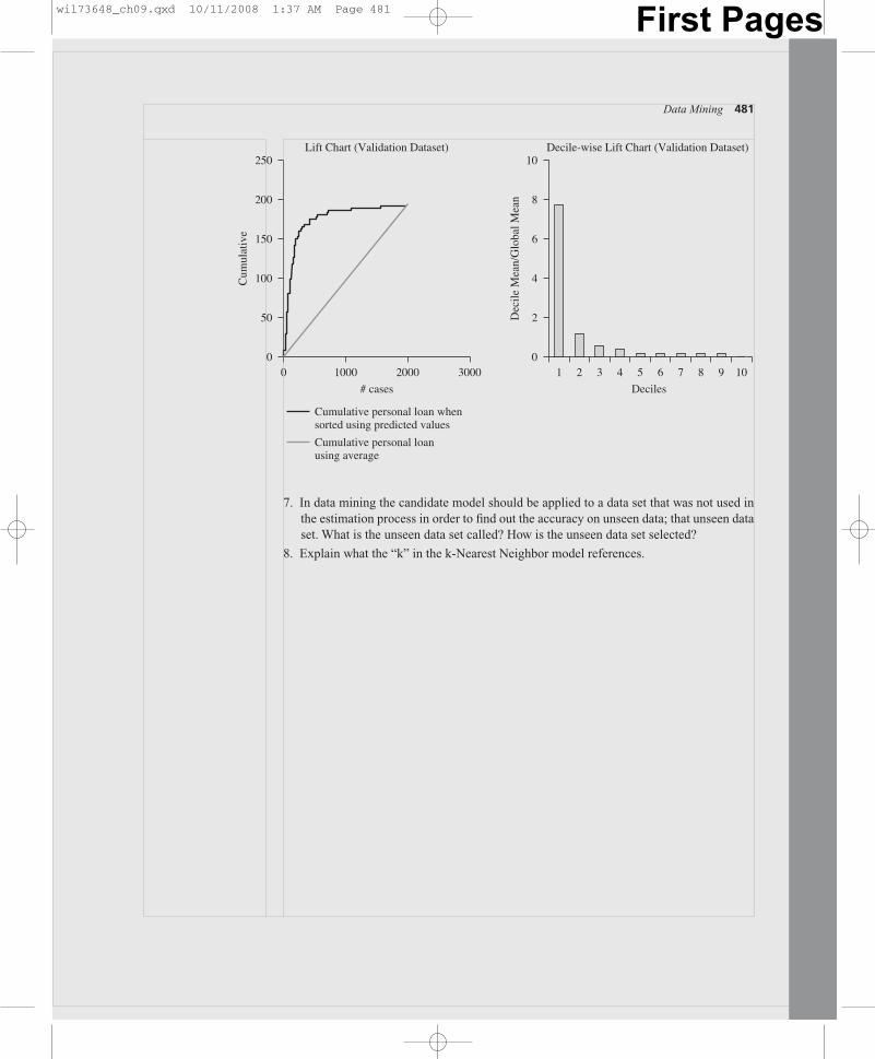
Data Mining 481

7. In data mining the candidate model should be applied to a data set that was not used inthe estimation process in order to find out the accuracy on unseen data; that unseen dataset. What is the unseen data set called? How is the unseen data set selected?

8. Explain what the “k” in the k-Nearest Neighbor model references.

00 1000 2000

# cases

3000

50

100

150C

umul

ativ

e

200

250




01 2 3 4 5 6 7 8 9 10

Deciles

4

2

6

8

Dec

ile M

ean/

Glo

bal M

ean



Documents

Chapter Nine - University of Notre Damebusiforc/handouts/Class_Notes/Chapter 9 Data Minin… · Chapter Nine Data Mining ... (perhaps unknown) intelligence or useful information from