Embed Size (px)
Citation preview

30
CHAPTER – III
CONSTRUCTION OF NEIGHBOUR DESIGNS FOR OS2 SERIES USING MOLS
3.1 Introduction
An individual’s phenotype (P) is the resultant effect of the genotype (G) of the
individual, the environment (E) that the individual is exposed to, and the interaction that
occurs between the genotype of the individual and the environment (G x E). Large G x E
effects tends to be viewed as problematic in breeding programme because of the lack of a
predictable response. This idealized predictable response across multiple environments is
generally referred to be stability. The term stability is used by the breeders to characterize
a genotype with a near constant yield irrespective of environments. One approach to
examine stability is to further partition the G x E interaction from a traditional Analysis
of Variance (ANOVA) into linear trends and a departure from linear (residual). Yates and
Cochran (1938) were the first to introduce the concept of stability parameters. Later on,
Finlay and Wilkinson (1963), Eberhart and Russell (1966), Perkins and Jinks (1968a, b),
Freeman and Perkins (1971) and Shukla (1972) used Variance Component approach for
finding stability parameters. Laxmi (1992) and Laxmi and Renu (2000) considered this
method for finding the stability measures for missing observations. They all obtained the
stability parameters for data whether complete or incomplete from experiments which
were conducted in multi-environment trials using different block designs. No one has
worked for neighbour designs to find the stability parameter.
To obtain a stability parameter one should go for the analysis of data using
variance component approach, which is one of the most common method used to identify
the existence of G x E interaction. For a statistical analysis of the data, an experimenter
should plan an appropriate experiment to obtain relevant information from it and Designs
of Experiments do this work successfully, which deals with planning, conducting,
analyzing and interpreting tests to evaluate the factors that control the value of a

31
parameter or group of parameters. The first step of experiments is planning which is
construction of design in statistical terminology.
Many of the current statistical approaches to designed experiments originate from
the work of R. A. Fisher in the early part of the 20th century. A strategically planned and
executed experiment may provide a great deal of information about the effect on a
variable due to one or more factors. Experiment can be designed in different ways in
which many experiments involve holding certain factors constant and altering the levels
of another variable. This One-Factor-at-a-Time approach is, however, inefficient when
compared with changing factor levels simultaneously. To overcome this problem, when
the number of treatments to be compared is less, the Latin Square or Randomized
Complete Block Designs are available and efficient. As the number of treatments
increases, these designs tend to become less homogenous, which is one of the most
important and basic principle for designing an experiment. In some experiment it is not
possible to use large size blocks accommodating all the treatments in each block. In that
case, we use an incomplete block design, i.e., a design in which the number of plots in a
block is less than the number of treatments. To compare pairs of treatments, with equal
accuracy treatments should occur in the same block an equal number of times and is
referred as balanced. Balanced Incomplete Block Designs (B.I.B.D) can be arranged only
for certain combinations of block size and number of replications. It is sometimes
important to arrange the treatments in field experimentation in such a way that at least
one replicate of every treatment is very near to at least one replicate of all the other
treatments to satisfy the condition of neighbour balance. If each block is a single line of
plots and blocks are well separated, extra parameters are needed for the effects of left and
right edges. For these extra parameters an alternative is to have border plots on both ends
of every block. Each border plot receives an experimental treatment, but it is not used for
measuring the response variable. When edge effects are very severe, such border plots are
always recommended; they do not add too much to the cost of experiments. The
arrangement of the border treatment at either end of the block is the same as the treatment

32
on the interior plot at the other end of the block then all the blocks of the designs is said
to be circular. The design constructed in such a way is known as neighbour design which
further may be completely neighbour balanced or partially neighbour balanced.
For the statistical analysis of the data, an experimenter should plan an appropriate
experiment i.e. should construct a design, in statistical terminology. In the present chapter
construction of neighbour design is discussed. Using the method of MOLS, BIBD of OS2
series with parameters v=b= s2+s+1, r=k=s+1, λ=1 is constructed, from which neighbour
design is obtained using circularity method. Finally, two-sided neighbours for a treatment
are observed and a systematic pattern for the neighbours has been given.
3.2 Construction of MOLS
A Latin square of order s is an s x s matrix whose entries are from a set of s
distinct treatments such that each treatment occurs exactly once in each row and column.
Two Latin squares A= [aij], B= [bij] of order s are Mutually Orthogonal Latin Squares
(MOLS) if the s 2 ordered pairs (aij, bij) are all distinct. A set A1,A2,…,An of Latin squares
of order s is called orthogonal if Ai and Aj are orthogonal for all i ≠j. It is easy to show
that the total number of MOLS, i.e., n ≤ s-1. An orthogonal set is said to be complete
provided if n=s-1 i.e. the total number of MOLS of order s can be at the most s-1.
When v = s is either a prime number or a prime power, elements of Galois Field
i.e. G.F.(s)are used as symbols for writing the Latin squares. The row and column
numbers in the first Latin square are obtained by adding the corresponding entries, (that
is occurring in the same position) of row and column mod(s). Let the v combinations be
written in arrow and again in a column so as to obtain the summation table of all possible
sums, two by two, of the row column combinations mod(s). This column will be called
the principal column and the row, the principal row. It can be easily seen that the
summation table gives a Latin square. The principal column in the second Latin square is
obtained by multiplying the entries in the first principal column of the first Latin square
by the elements of G.F.(s), say, (a1, a2,…,ap), where ai≠ 0 or 1. The contents of second
33
Latin square are then obtained by adding the corresponding entries of row and column
(mod s). Again a third principal column is obtained by multiplying the different elements
by the first principal column by another element of G.F.(s), say, (b1, b2,…,bp), where bi≠
ai , or 0 or 1 (i = 1,2,…,p), i.e., the multiplier is so chosen that no element is repeated.
The contents of third Latin square are then obtained by adding the corresponding entries
of row and column (mod s). This square is orthogonal to previous two and this process is
continued till suitable multipliers are available.
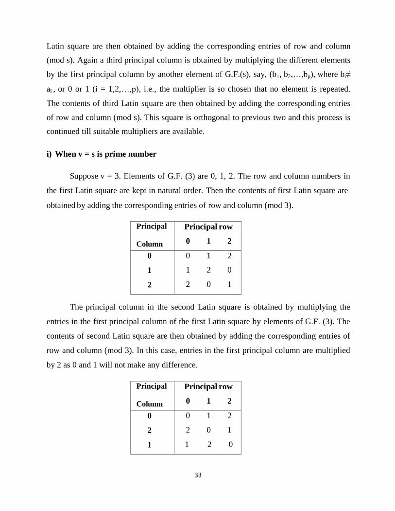
i) When v = s is prime number
Suppose v = 3. Elements of G.F. (3) are 0, 1, 2. The row and column numbers in
the first Latin square are kept in natural order. Then the contents of first Latin square are
obtained by adding the corresponding entries of row and column (mod 3).
Principal
Column
Principal row
0 1 2
0
1
2
0 1 2
1 2 0
2 0 1
The principal column in the second Latin square is obtained by multiplying the
entries in the first principal column of the first Latin square by elements of G.F. (3). The
contents of second Latin square are then obtained by adding the corresponding entries of
row and column (mod 3). In this case, entries in the first principal column are multiplied
by 2 as 0 and 1 will not make any difference.
Principal
Column
Principal row
0 1 2
0
2
1
0 1 2
2 0 1
1 2 0

34
Therefore, a complete set of MOLS for v = 3:
I II
0
1
2
0
1
2
1 2 0 2 0 1
2 0 1 1 2 0
ii) When v is prime power
Let v = 22
= 4. The elements in the G.F. (22) are 0, 1, α, α
2 (= α+1) with α
2 + α+1 =
0 as the minimal function and α as a primitive element of G.F.
The principal row and column of the first Latin square is taken in natural order.
Then the contents of first Latin square are obtained by adding the corresponding entries
of row and column (mod 2).
Principal
column
Principal row
0 1 α α+1
0
1
α
α+1
0 1 α α+1
1 0 α+1 α
α α+1 0 1
α+1 α 1 0
The principal column for the second Latin square is obtained by multiplying the
entries in the first principal column of the first Latin square by α. The contents of second
Latin square are then obtained by adding the corresponding entries of row and column
(mod 2).
35
Principal
Column
Principal row
0 1 α α+1
0
α
α+1
1
0 1 α α+1
α α+1 0 1
α+1 α 1 0
1 0 α+1 α
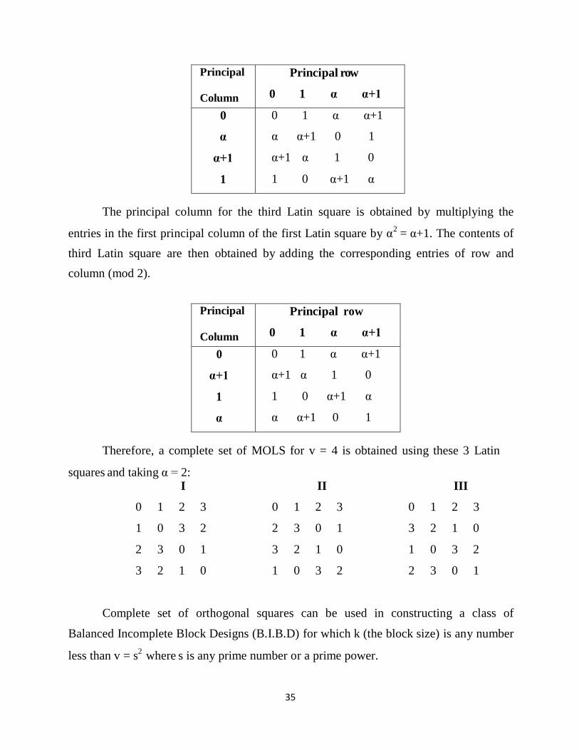
The principal column for the third Latin square is obtained by multiplying the
entries in the first principal column of the first Latin square by α2
= α+1. The contents of
third Latin square are then obtained by adding the corresponding entries of row and
column (mod 2).
Principal
Column
Principal row
0 1 α α+1
0
α+1
1
α
0 1 α α+1
α+1 α 1 0
1 0 α+1 α
α α+1 0 1
Therefore, a complete set of MOLS for v = 4 is obtained using these 3 Latin
squares and taking α = 2: I II III
0 1 2 3 0 1 2 3 0 1 2 3
1 0 3 2 2 3 0 1 3 2 1 0
2 3 0 1 3 2 1 0 1 0 3 2
3 2 1 0 1 0 3 2 2 3 0 1
Complete set of orthogonal squares can be used in constructing a class of
Balanced Incomplete Block Designs (B.I.B.D) for which k (the block size) is any number
less than v = s2
where s is any prime number or a prime power.

36
3.3 Construction of BIB Designs
An Incomplete Block Design with v treatments distributed over b blocks, each of
size k(< v) such that each treatment occurs in r blocks, no treatment occurs more than
once in a block and each pair of treatments occurs together in λ blocks, is called a
Balanced Incomplete Block Designs (B.I.B.D). So the existence of a complete set of
squares of order s is equivalent to the existence of a BIBD with parameters v= s2, b=
s(s+1), r= s+1, k=s, λ=1. The BIB design series with parameters; v= s2, b= s(s+1), r= s+1,
k=s, λ=1 and v=b= s2+s+1, r=k=s+1, λ=1 are orthogonal series of BIB Designs which
were given by Yates (1936). In general, the first series is known as OS1 series and the
second series is known as OS2 series. Here the OS1 series is the residual of the OS2
series for a given s. It had been shown by Yates that the solution of OS1 series is always
affine-α resolvable as k2/v is an integer. If a resolvable solution exists for OS1, then OS2
series can be constructed from it. Now, the BIB Designs with the parameters v= s2, b=
s(s+1), r= s+1, k=s, λ=1with the help of complete sets of MOLS can be constructed as
discussed in the following section.
3.3.1 Construction of OS1 Series
Let there be v= s2
(s is a prime number or a prime power) treatments, numbered as 1,
2, …, s2. Arrange these treatment numbers in the form of a s x s square array in natural
order, i.e., in a standard array (say L). The sets/ blocks S1, S2,…, Ss(s+1); which constitute
the BIB Design with parameters v=s2, b= s(s+1), r= s+1, k=s and λ=1 can be constructed
by writing the symbols as follows:
i) The ith set contains the symbols occurring in the ith block of L (i=1,2,…,s)
ii) The (s+j)th set contains the symbols occurring in the jth column of L (j=1, 2,…, s).
iii) Let L1, L2,…, Ls-1, be a complete set of MOLS of order s. On superimposing Lα
on L, the symbols corresponding to the k-th letter of Lα constitute the set S{(α+1)s+k}
where k=1,2,…,s and α=1,2,…,s-1.
37
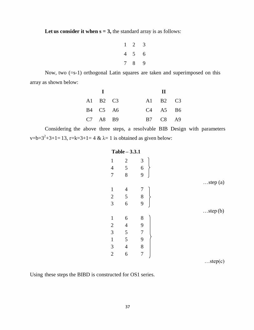
Let us consider it when s = 3, the standard array is as follows:
1 2 3
4 5 6
7 8 9
Now, two (=s-1) orthogonal Latin squares are taken and superimposed on this
array as shown below:
I II
A1 B2 C3 A1 B2 C3
B4 C5 A6 C4 A5 B6
C7 A8 B9 B7 C8 A9
Considering the above three steps, a resolvable BIB Design with parameters
v=b=32+3+1= 13, r=k=3+1= 4 & λ= 1 is obtained as given below:
Table – 3.3.1
1 2 3
…step (a)
…step (b)
4 5 6
7
1
8
4
9
7
2 5 8
3
1
6
6
9
8
2 4 9
3 5 7
1 5 9
3 4 8
2 6 7
…step(c)
Using these steps the BIBD is constructed for OS1 series.
38
3.3.2 Construction of OS2 Series
According to the properties of MOLS, the design so constructed is affine-
resolvable solution of the BIB design with the parameters given by series OS1. As OS1
series is the residual of OS2 series and affine-resolvable thus the solution for OS2 series
can be given by adding a new symbol θi to each set of the ith replication (i=1,2,…,s+1) in
such a way that θ1 is the (s2+1)
th treatment. This θ1 becomes the last column of the design
for first s block, then θ2 i.e. (s2+2)
th treatment becomes last column for next s block and
so on. This new symbol also gave a new set (θ1, θ2,…, θs+1) which become last block of
the design. By adding new symbol θi in this way all the conditions for BIB design has
been fulfilled and this constitutes OS2 series directly from OS1 series without
constructing the actual design. The said series of BIB Designs with the parameters can be
constructed when s is a prime number or prime power.
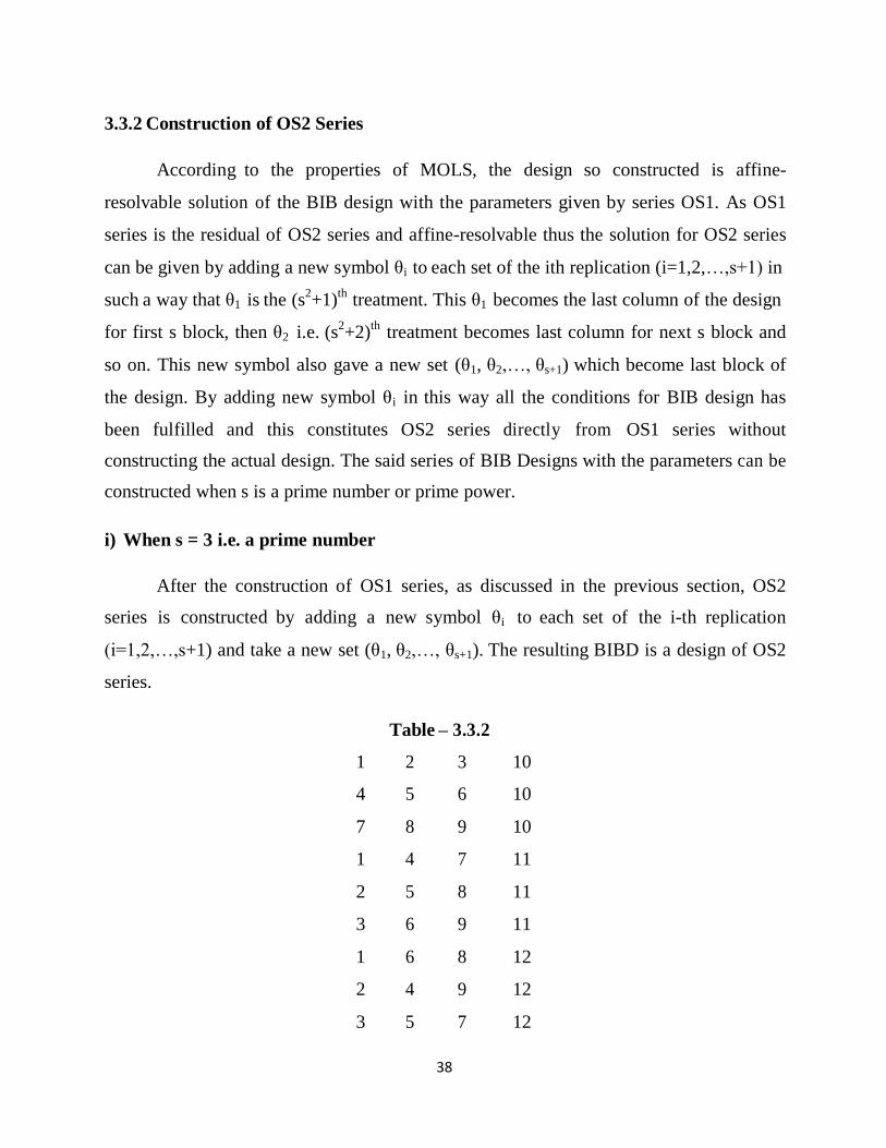
i) When s = 3 i.e. a prime number
After the construction of OS1 series, as discussed in the previous section, OS2
series is constructed by adding a new symbol θi to each set of the i-th replication
(i=1,2,…,s+1) and take a new set (θ1, θ2,…, θs+1). The resulting BIBD is a design of OS2
series.
Table – 3.3.2
1 2 3 10
4 5 6 10
7 8 9 10
1 4 7 11
2 5 8 11
3 6 9 11
1 6 8 12
2 4 9 12
3 5 7 12
39
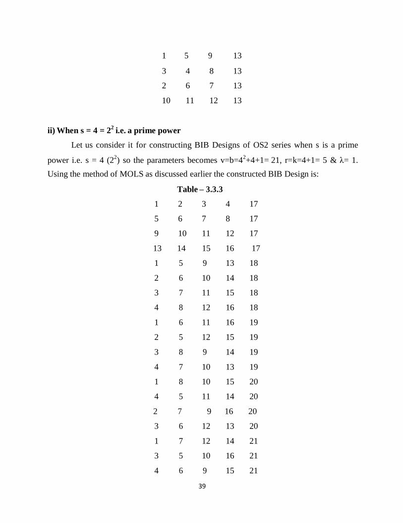
1 5 9 13
3 4 8 13
2 6 7 13
10 11 12 13
ii) When s = 4 = 22
i.e. a prime power
Let us consider it for constructing BIB Designs of OS2 series when s is a prime
power i.e. s = 4 (22) so the parameters becomes v=b=4
2+4+1= 21, r=k=4+1= 5 & λ= 1.
Using the method of MOLS as discussed earlier the constructed BIB Design is:
Table – 3.3.3
1 2 3 4 17
5 6 7 8 17
9 10 11 12 17
13 14 15 16 17
1 5 9 13 18
2 6 10 14 18
3 7 11 15 18
4 8 12 16 18
1 6 11 16 19
2 5 12 15 19
3 8 9 14 19
4 7 10 13 19
1 8 10 15 20
4 5 11 14 20
2 7 9 16 20
3 6 12 13 20
1 7 12 14 21
3 5 10 16 21
4 6 9 15 21

40
2 8 11 13 21
17 18 19 20 21
Using the method of MOLS the BIB Designs for OS2 series can be constructed for
any value of s whether s is a prime number or a prime power.
3.4 Construction of Neighbour Designs for OS2 Series
After the construction of BIBD, Rees (1967) suggested construction of neighbour
designs by using the border plots, that is, one plot is added at each end of each block.
Arrangement of treatments at border plots at either end of the block are the same as the
treatment on the interior plot at the other end of block and not used for measuring the
response variable. Plots other than border plots are described as internal plots for
neighbour designs. In this neighbour design, all the blocks shall be circular in the sense
that the border treatments at either end of the block are the same as the treatment on the
interior plot at the other end of block. For a design d, d(i, j) denotes the treatment applied
to plot j of block i, particularly, d(i, 0) and d(i, k+1) are the two treatments applied to the
border plots of block i and the circularity condition implies that d(i, 0)= d(i, k) and d(i,
k+1)= d(i, 1) ; where 1≤ i≤ b &1≤ j ≤ k. These extra parameters used as neighbour plots
are needed for the effect of left and right neighbours. Now consider the construction of
neighbour design for OS2 series for any value of s whether s is a prime number or a
prime power.
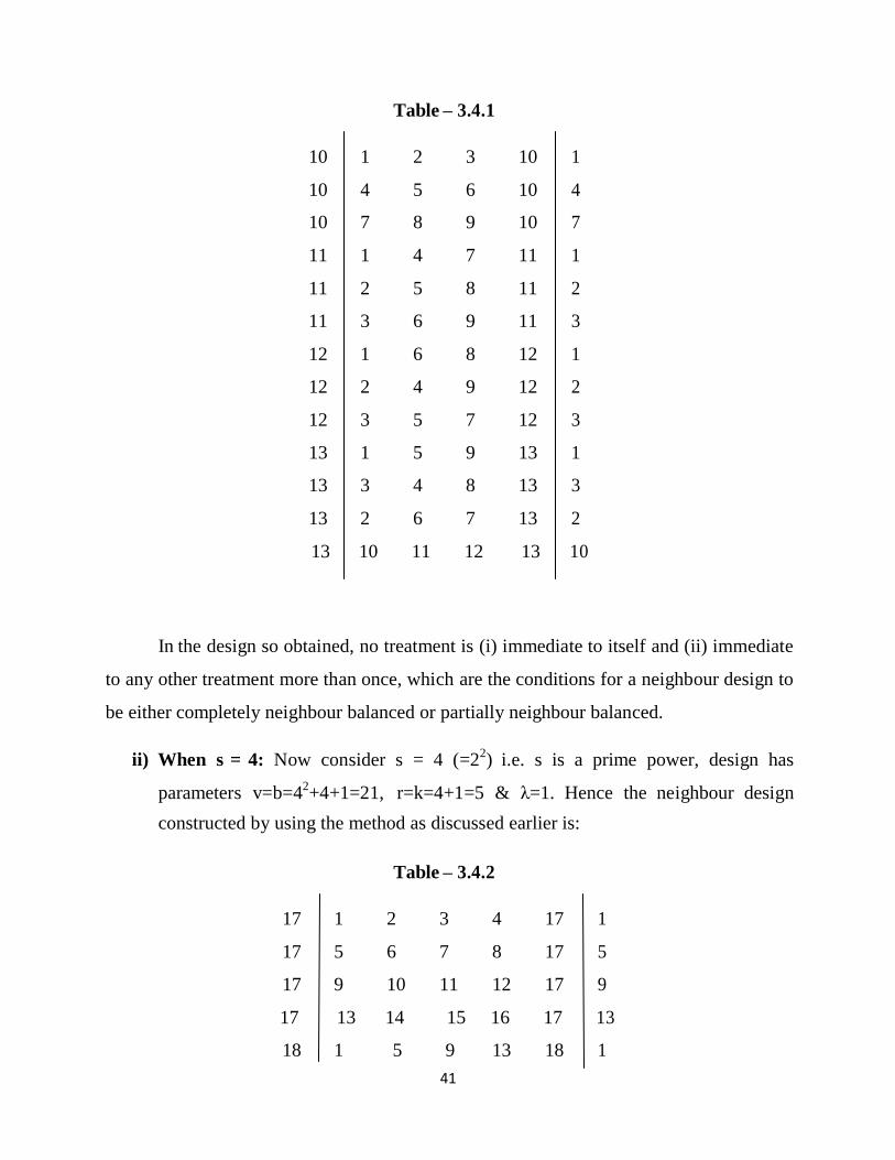
i) When s = 3: As s is a prime number i.e. s = 3, design has parameters v=b=32+3+1
=13, r=k=3+1=4 and λ=1. In the design d(i,0) and d(i,5) are the two treatments
which are applied to the border plots of block i where d(i, 0)= d(i, 4) and d(i, 5)=
d(i, 1); 1≤ i≤ 13 which fulfill the circularity conditions. Hence the resulting design
is a neighbour design:
41
Table – 3.4.1
10 1 2 3 10 1
10 4 5 6 10 4
10 7 8 9 10 7
11 1 4 7 11 1
11 2 5 8 11 2
11 3 6 9 11 3
12 1 6 8 12 1
12 2 4 9 12 2
12 3 5 7 12 3
13 1 5 9 13 1
13 3 4 8 13 3
13 2 6 7 13 2
13 10 11 12 13 10
In the design so obtained, no treatment is (i) immediate to itself and (ii) immediate
to any other treatment more than once, which are the conditions for a neighbour design to
be either completely neighbour balanced or partially neighbour balanced.
ii) When s = 4: Now consider s = 4 (=22) i.e. s is a prime power, design has
parameters v=b=42+4+1=21, r=k=4+1=5 & λ=1. Hence the neighbour design
constructed by using the method as discussed earlier is:
Table – 3.4.2
17 1 2 3 4 17 1
17 5 6 7 8 17 5
17 9 10 11 12 17 9
17 13 14 15 16 17 13
18 1 5 9 13 18 1

42
18 2 6 10 14 18 2
18 3 7 11 15 18 3
18 4 8 12 16 18 4
19 1 6 11 16 19 1
19 2 5 12 15 19 2
19 3 8 9 14 19 3
19 4 7 10 13 19 4
20 1 8 10 15 20 1
20 4 5 11 14 20 4
20 2 7 9 16 20 2
20 3 6 12 13 20 3
21 1 7 12 14 21 1
21 3 5 10 16 21 3
21 4 6 9 15 21 4
21 2 8 11 13 21 2
21 17 18 19 20 21 17
In the design so obtained, again no treatment is (i) immediate to itself and (ii)
immediate to any other treatment more than once and shows that the neighbour design is
either completely neighbour balanced or partially neighbour balanced. Here again all the
blocks are circular in the sense that the border treatments at either end of the block is the
same as the treatment on the interior plot at the other end of block i.e. d(i, 0)= d(i, 5) and
d(i, 6)= d(i, 1) ; where 1≤ i≤ 21. Similarly the neighbour designs for s =5, 23=8, 3
2=9, 11
and so on, can be constructed in the same way.
3.5 Neighbours of Treatment for Neighbour Designs of OS2 Series
For the analysis of two-sided neighbour designs, left neighbours and right
neighbours of a treatment must be known. So let us consider firstly the left neighbours of
a treatment in neighbour designs of OS2 series.
43
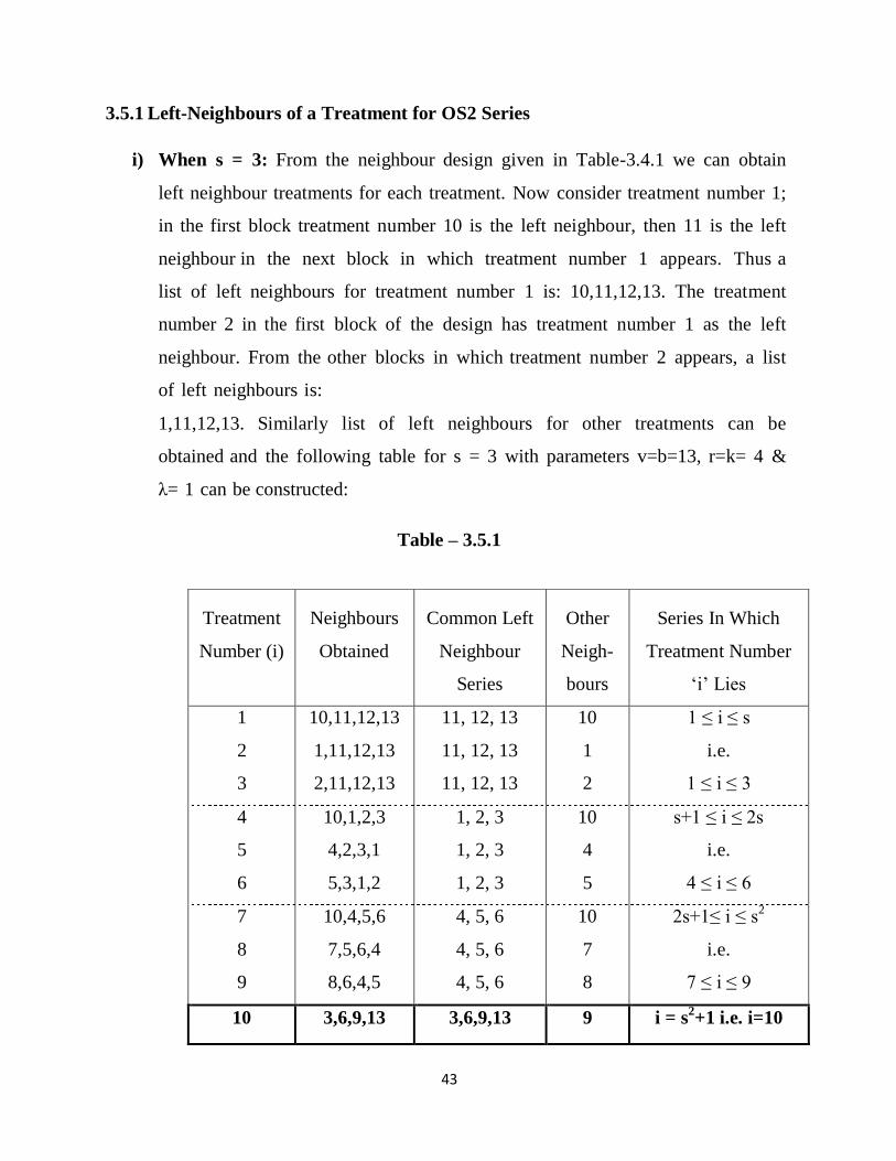
3.5.1 Left-Neighbours of a Treatment for OS2 Series
i) When s = 3: From the neighbour design given in Table-3.4.1 we can obtain
left neighbour treatments for each treatment. Now consider treatment number 1;
in the first block treatment number 10 is the left neighbour, then 11 is the left
neighbour in the next block in which treatment number 1 appears. Thus a
list of left neighbours for treatment number 1 is: 10,11,12,13. The treatment
number 2 in the first block of the design has treatment number 1 as the left
neighbour. From the other blocks in which treatment number 2 appears, a list
of left neighbours is:
1,11,12,13. Similarly list of left neighbours for other treatments can be
obtained and the following table for s = 3 with parameters v=b=13, r=k= 4 &
λ= 1 can be constructed:
Table – 3.5.1
Treatment
Number (i)
Neighbours
Obtained
Common Left
Neighbour
Series
Other
Neigh-
bours
Series In Which
Treatment Number
‘i’ Lies
1
2
3
10,11,12,13
1,11,12,13
2,11,12,13
11, 12, 13
11, 12, 13
11, 12, 13
10
1
2
1 ≤ i ≤ s
i.e.
1 ≤ i ≤ 3
4
5
6
10,1,2,3
4,2,3,1
5,3,1,2
1, 2, 3
1, 2, 3
1, 2, 3
10
4
5
s+1 ≤ i ≤ 2s
i.e.
4 ≤ i ≤ 6
7
8
9
10,4,5,6
7,5,6,4
8,6,4,5
4, 5, 6
4, 5, 6
4, 5, 6
10
7
8
2s+1≤ i ≤ s2
i.e.
7 ≤ i ≤ 9
10 3,6,9,13 3,6,9,13 9 i = s2+1 i.e. i=10
44
It should be noted here that each treatment has 4 = (s+1) treatments which are left
neighbours. From the above table we observe that the treatment number 1 has s = 3
neighbours 11, 12, 13 as common left neighbour series which can be written as s2+2, s
2+3
(or s2+s), s
2+4 (or s
2+s+1). One more left neighbour of treatment i=1 is observed as 10. The
left neighbour means i-1. Here i-1 =0(mod v) = 13 has already occurred as one of the
members in the left common series. So the repeated treatment number is replaced by the
treatment number 10 which may be written as treatment number s2+1. The left common
series of ‘s’ treatments is immediately previous series of the series in which treatment
number ‘i’ lies, assuming the treatment in circular way.
The treatment number 2 has s = 3 neighbours 11, 12, 13 which is again left common
neighbour series for i-th treatment (1 ≤ i ≤ s). Again the left neighbour series 11, 12, 13 can
be written as s2+2, s
2+3 (or s
2+s), s
2+4 (or s
2+s+1). As noticed earlier, there shall be 4 left
neighbours for each treatment, so one more left neighbour of treatment number i=2
observed is 1 which may be written as i-1.
Let us consider treatment number 3 or i = s. It has s = 3 neighbours 11, 12, 13 as the
common left neighbour series of i-th treatment (1 ≤ i ≤ s). Here again these can be written
as s2+2, s
2+3 (or s
2+s), s
2+4 (or s
2+s+1). Again the one more left neighbour treatment of
treatment number i=3 observed is 2 can be written as i-1.
The treatment number 4 or i = s+1 has s = 3 neighbours 1, 2, 3 which is common left
neighbour series of the i-th treatment (s+1 ≤ i ≤ 2s). Now the left neighbours 1, 2, 3 can be
written as series 1, … , s. The one more left neighbour treatment of treatment number i=4 is
observed as 10. According to the perception this should be i-1 i.e. 3. But treatment number
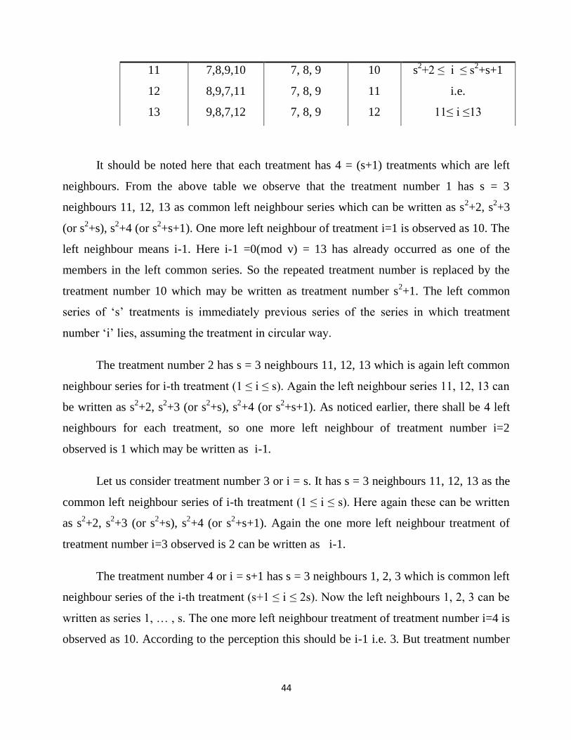
11
12
13
7,8,9,10
8,9,7,11
9,8,7,12
7, 8, 9
7, 8, 9
7, 8, 9
10
11
12
s2+2 ≤ i ≤ s
2+s+1
i.e.
11≤ i ≤13
45
3 has already occurred as one of the members in the left series. Now it is replaced by the
treatment number 10 i.e. s2+1.
Now consider treatment number 5 or i =s+2 has s = 3 neighbours 1, 2, 3 again as
common left neighbour series of the i-th treatment (s+1 ≤ i ≤ 2s). The one more left
neighbour treatment of treatment number i=5 is 4 which can be written as i-1.
Let us consider treatment number 6 or i =2s has s = 3 neighbours 1, 2, 3 again as
common left neighbour series of the i-th treatment (s+1 ≤ i ≤ 2s). The one more left
neighbour treatment of treatment number i=1 is 5, which is written as i-1.
The treatment number 7 or i =2s+1 has s = 3 neighbours 4, 5, 6 as the common left
neighbour series of the i-th treatment (2s+1 ≤ i ≤ 3s or s2). Now the left neighbours 4, 5, 6
can be written as s+1, … , s+s(=2s). The one more left neighbour treatment of treatment
number i=7 is 10. It should be according to the perception i-1 i.e. 6. But treatment number 6
has already occurred as one of the members in the left series. So it is replaced by the
treatment number 10 i.e. s2+1. So it may be percepted that one left neighbour of i-th
treatment is i-1. If this occurs in the already obtained ‘s’ common left neighbours of the i-
th treatment, it may be replaced by the treatment number s2+1.
Consider the treatment number 8 or i =2s+2 has s = 3 neighbours 4, 5, 6 which is
common left neighbour series of the i-th treatment (2s+1 ≤ i ≤ 3s or s2). The one more left
neighbour treatment of treatment number i=8 is observed as 7 which is written as i-1.
Now the treatment number 9 or i = s2 has s = 3 neighbours 4, 5, 6 which is common
left neighbour series of the i-th treatment (2s+1 ≤ i ≤ 3s or s2). The one more left neighbour
treatment of treatment number i=9 is 8 which is written as i-1.
We observed that treatment number 10 or i = s2+1 has neighbours which are entirely
different from the series and the conception, so we shall discuss it later.
46
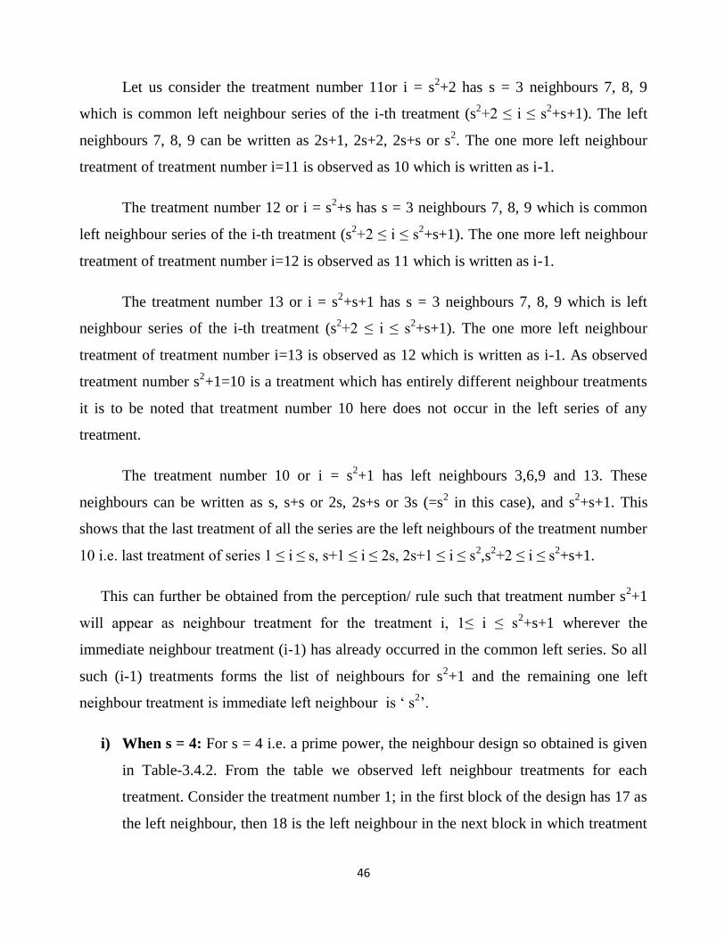
Let us consider the treatment number 11or i = s2+2 has s = 3 neighbours 7, 8, 9
which is common left neighbour series of the i-th treatment (s2+2 ≤ i ≤ s
2+s+1). The left
neighbours 7, 8, 9 can be written as 2s+1, 2s+2, 2s+s or s2. The one more left neighbour
treatment of treatment number i=11 is observed as 10 which is written as i-1.
The treatment number 12 or i = s2+s has s = 3 neighbours 7, 8, 9 which is common
left neighbour series of the i-th treatment (s2+2 ≤ i ≤ s
2+s+1). The one more left neighbour
treatment of treatment number i=12 is observed as 11 which is written as i-1.
The treatment number 13 or i = s2+s+1 has s = 3 neighbours 7, 8, 9 which is left
neighbour series of the i-th treatment (s2+2 ≤ i ≤ s
2+s+1). The one more left neighbour
treatment of treatment number i=13 is observed as 12 which is written as i-1. As observed
treatment number s2+1=10 is a treatment which has entirely different neighbour treatments
it is to be noted that treatment number 10 here does not occur in the left series of any
treatment.
The treatment number 10 or i = s2+1 has left neighbours 3,6,9 and 13. These
neighbours can be written as s, s+s or 2s, 2s+s or 3s (=s2 in this case), and s
2+s+1. This
shows that the last treatment of all the series are the left neighbours of the treatment number
10 i.e. last treatment of series 1 ≤ i ≤ s, s+1 ≤ i ≤ 2s, 2s+1 ≤ i ≤ s2,s
2+2 ≤ i ≤ s
2+s+1.
This can further be obtained from the perception/ rule such that treatment number s2+1
will appear as neighbour treatment for the treatment i, 1≤ i ≤ s2+s+1 wherever the
immediate neighbour treatment (i-1) has already occurred in the common left series. So all
such (i-1) treatments forms the list of neighbours for s2+1 and the remaining one left
neighbour treatment is immediate left neighbour is ‘ s2’.
i) When s = 4: For s = 4 i.e. a prime power, the neighbour design so obtained is given
in Table-3.4.2. From the table we observed left neighbour treatments for each
treatment. Consider the treatment number 1; in the first block of the design has 17 as
the left neighbour, then 18 is the left neighbour in the next block in which treatment
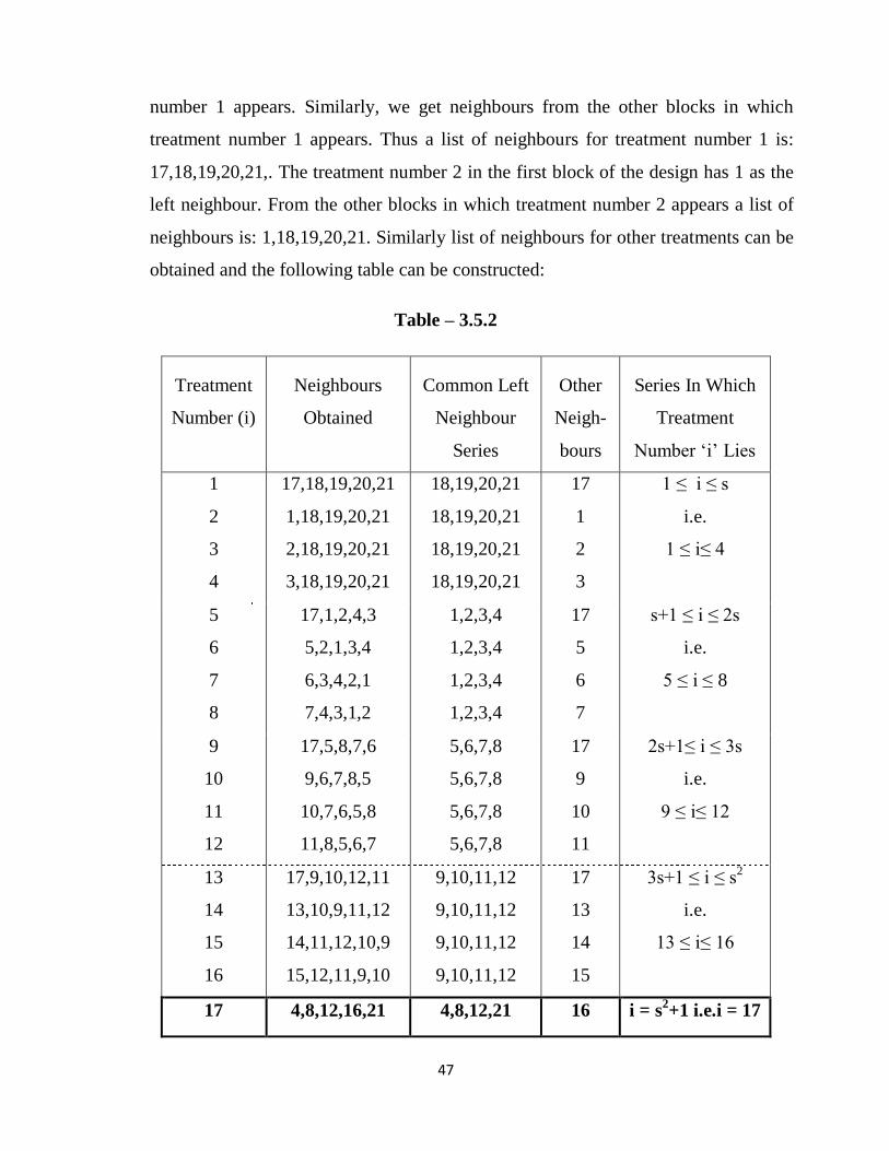
47
number 1 appears. Similarly, we get neighbours from the other blocks in which
treatment number 1 appears. Thus a list of neighbours for treatment number 1 is:
17,18,19,20,21,. The treatment number 2 in the first block of the design has 1 as the
left neighbour. From the other blocks in which treatment number 2 appears a list of
neighbours is: 1,18,19,20,21. Similarly list of neighbours for other treatments can be
obtained and the following table can be constructed:
Table – 3.5.2
Treatment
Number (i)
Neighbours
Obtained
Common Left
Neighbour
Series
Other
Neigh-
bours
Series In Which
Treatment
Number ‘i’ Lies
1
2
3
4
17,18,19,20,21
1,18,19,20,21
2,18,19,20,21
3,18,19,20,21
18,19,20,21
18,19,20,21
18,19,20,21
18,19,20,21
17
1
2
3
1 ≤ i ≤ s
i.e.
1 ≤ i≤ 4
5
6
7
8
17,1,2,4,3
5,2,1,3,4
6,3,4,2,1
7,4,3,1,2
1,2,3,4
1,2,3,4
1,2,3,4
1,2,3,4
17
5
6
7
s+1 ≤ i ≤ 2s
i.e.
5 ≤ i ≤ 8
9
10
11
12
17,5,8,7,6
9,6,7,8,5
10,7,6,5,8
11,8,5,6,7
5,6,7,8
5,6,7,8
5,6,7,8
5,6,7,8
17
9
10
11
2s+1≤ i ≤ 3s
i.e.
9 ≤ i≤ 12
13
14
15
16
17,9,10,12,11
13,10,9,11,12
14,11,12,10,9
15,12,11,9,10
9,10,11,12
9,10,11,12
9,10,11,12
9,10,11,12
17
13
14
15
3s+1 ≤ i ≤ s2
i.e.
13 ≤ i≤ 16
17 4,8,12,16,21 4,8,12,21 16 i = s2+1 i.e.i = 17
48
18
19
20
21
13,14,15,16,17
16,15,14,13,18
15,14,16,13,19
14,16,15,13,20
13,14,15,16
13,14,15,16
13,14,15,16
13,14,15,16
17
18
19
20
s2+2 ≤ i ≤ s
2+s+1
i.e
18 ≤ i≤ 21
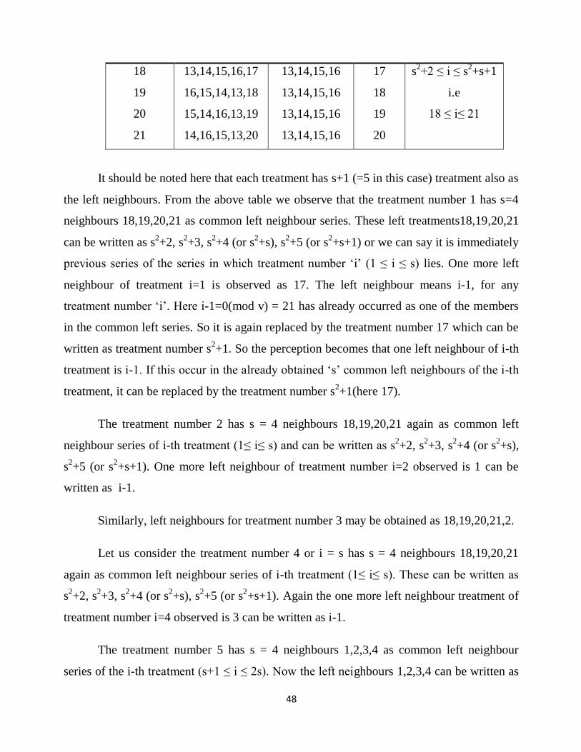
It should be noted here that each treatment has s+1 (=5 in this case) treatment also as
the left neighbours. From the above table we observe that the treatment number 1 has s=4
neighbours 18,19,20,21 as common left neighbour series. These left treatments18,19,20,21
can be written as s2+2, s
2+3, s
2+4 (or s
2+s), s
2+5 (or s
2+s+1) or we can say it is immediately
previous series of the series in which treatment number ‘i’ (1 ≤ i ≤ s) lies. One more left
neighbour of treatment i=1 is observed as 17. The left neighbour means i-1, for any
treatment number ‘i’. Here i-1=0(mod v) = 21 has already occurred as one of the members
in the common left series. So it is again replaced by the treatment number 17 which can be
written as treatment number s2+1. So the perception becomes that one left neighbour of i-th
treatment is i-1. If this occur in the already obtained ‘s’ common left neighbours of the i-th
treatment, it can be replaced by the treatment number s2+1(here 17).
The treatment number 2 has s = 4 neighbours 18,19,20,21 again as common left
neighbour series of i-th treatment (1≤ i≤ s) and can be written as s2+2, s
2+3, s
2+4 (or s
2+s),
s2+5 (or s
2+s+1). One more left neighbour of treatment number i=2 observed is 1 can be
written as i-1.
Similarly, left neighbours for treatment number 3 may be obtained as 18,19,20,21,2.
Let us consider the treatment number 4 or i = s has s = 4 neighbours 18,19,20,21
again as common left neighbour series of i-th treatment (1≤ i≤ s). These can be written as
s2+2, s
2+3, s
2+4 (or s
2+s), s
2+5 (or s
2+s+1). Again the one more left neighbour treatment of
treatment number i=4 observed is 3 can be written as i-1.
The treatment number 5 has s = 4 neighbours 1,2,3,4 as common left neighbour
series of the i-th treatment (s+1 ≤ i ≤ 2s). Now the left neighbours 1,2,3,4 can be written as
49
1,…, s. One more left neighbour treatment of treatment number i=5 observed is 17.
According to the perception it should be i-1 i.e. 4. As the treatment number 4 has already
occurred as one of the members in common left neighbour series, so it should be replaced
by the treatment number s2+1=17, which shows that the perception is true.
Using the same pattern, neighbours for the treatment numbers 6; 7 and 8 are
1,2,3,4,5;1,2,3,4,6 and 1,2,3,4,7 respectively.
Consider the treatment number 9 or i=9 i.e. ‘2s+1’ has s = 4 neighbours 5,6,7,8 as
common left neighbour series of the i-th treatment (s+1 ≤ i ≤ 2s). Now the left neighbours
5,6,7,8 can be written as s+1, s+2, s+3, s+4 (or s+s=2s). One more left treatment of
treatment number i=9 observed is 17. It should be according to the perception i-1 i.e. 8. As
the treatment number 8 has already occurred as one of the members in common left series.
So it is replaced by the treatment number s2+1=17 which shows that our perception is true.
In the same way, neighbours for the treatment numbers10; 11and 12 are 5,6,7,8,9;
5,6,7,8,10 and 5,6,7,8,11 respectively.
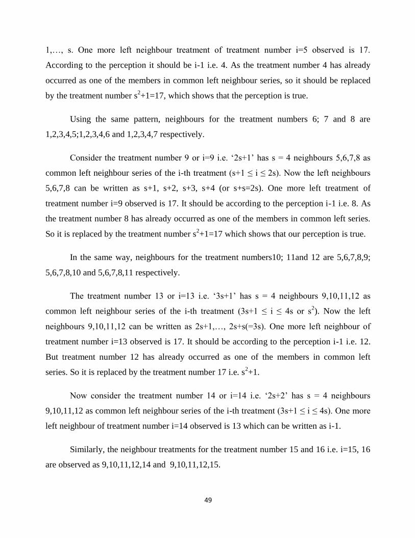
The treatment number 13 or i=13 i.e. ‘3s+1’ has s = 4 neighbours 9,10,11,12 as
common left neighbour series of the i-th treatment (3s+1 ≤ i ≤ 4s or s2). Now the left
neighbours 9,10,11,12 can be written as 2s+1,…, 2s+s(=3s). One more left neighbour of
treatment number i=13 observed is 17. It should be according to the perception i-1 i.e. 12.
But treatment number 12 has already occurred as one of the members in common left
series. So it is replaced by the treatment number 17 i.e. s2+1.
Now consider the treatment number 14 or i=14 i.e. ‘2s+2’ has s = 4 neighbours
9,10,11,12 as common left neighbour series of the i-th treatment (3s+1 ≤ i ≤ 4s). One more
left neighbour of treatment number i=14 observed is 13 which can be written as i-1.
Similarly, the neighbour treatments for the treatment number 15 and 16 i.e. i=15, 16
are observed as 9,10,11,12,14 and 9,10,11,12,15.
50
For s = 4 we again observed that treatment number 17 i.e. ‘s2+1’ has neighbours
which are entirely different from the series and the conception, so we shall discuss it later.
Let us consider the treatment number 18 or i=18 i.e. ‘s2+2’ has s = 4 neighbours
13,14,15,16 which is common left neighbour series of the i-th treatment (s2+2 ≤ i ≤
s2+s+1The left neighbours 13, 14, 15, 16 can be written as 3s+1, 3s+2, 3s+3, 3s+s (or 4s=s
2
here). One more left neighbour of treatment number i=18 observed is 17 which can be
written as i-1. As observed treatment number s2+1=17 is a treatment which has entirely
different neighbour treatments. It is also observed here it does not occur in common left
neighbour series of any treatment.
The treatment number 19 or i=19 i.e. ‘s2+3’ has s = 4 neighbours 13,14,15,16 as
common left neighbour series of the i-th treatment (s2+2 ≤ i ≤ s
2+s+1). One more left
neighbour of treatment number i=19 observed is 18 which can be written as i-1.
In the same way, the neighbours for the treatment number 20 and 21 are
13,14,15,16,19 and 13,14,15, 16,20.
The treatment number 17 or i=17 i.e. ‘s2+1’ has the neighbours 4,8,12,16,21. These
neighbours can be written as s, 2s, 3s, 4s (or s2 in this case), and s
2+s+1. This shows that the
last treatments of all the series are the left neighbours of the treatment number 17 i.e. 1 ≤ i
≤ s, s+1 ≤ i ≤ 2s, 2s+1≤ i ≤ 3s, 3s+1 ≤ i ≤ s2, s
2+2 ≤ i ≤ s
2+s+1.
This can further be obtained from the perception/ principle such that treatment
number s2+1 will appear as neighbour treatment for the treatment i, 1≤ i ≤ s
2+s+1 wherever
the immediate neighbour treatment (i-1) has already occurred in common left neighbour
series. So all such treatments for which the rule holds form the list of neighbours for
treatment number s2+1. The remaining one left neighbour treatment is left immediate
neighbour of treatment number i= s2+1 is ‘s
2’.

51
ii) Steps to find Left Neighbours
a) Observe the treatment number ‘i’, where i ≠ s2+1.
b) Then find the series in which the treatment number ‘i’ lies.
The series is defined in such a way that the sequence of first ‘s’ treatments of the
design form the first series, the sequence of next ‘s’ treatments i.e. ‘s+1’ to ‘2s’ form
the second series and so on up to ‘s2’. Thus have ‘s’ series up to the treatment
number ‘s2’. The last series i.e. ‘s+1’–th series of ‘s’ treatments always starts from
treatment number ‘s2+2’ instead of the treatment number ‘s
2+1’ and ended on
treatment number ‘s2+s+1’ for any ‘s’ whether it is a prime number or prime power.
It is due to the reason that whenever an immediate left-neighbour of i-th treatment
i.e. i-1 occurs already in the common left neighbour series then that repeated
treatment is replaced by the treatment number ‘s2+1’. Now the ‘s+2’-th series of next
‘s’ treatments shall be ‘s2+s+2’ to ‘s
2+2s+1’, which with mod(v) reduces to ‘1’ to
‘s’. So the s+2-th series is again the first series of the design. This again holds that
the design is circular.
c) Then find out the common left neighbour series for that treatment.
Let the treatment number ‘i’ lies in the j-th series (j=1,2,…,s+1), then ‘j-1’-th series
is the previous series which is the common left neighbour series.
d) One more left neighbour treatment can be find by the concept of neighbour that
means immediate.
This should be i-1 for the treatment number ‘i’. If this left treatment already occurs
in the common left neighbour series then that ‘i-1’–th treatment is replaced by the
treatment number s2+1. For neighbour design with parameters v=b=s
2+s+1, r=k=s+1
& λ=1, there shall always be s+1 treatments for each treatment as the left
neighbours.
52
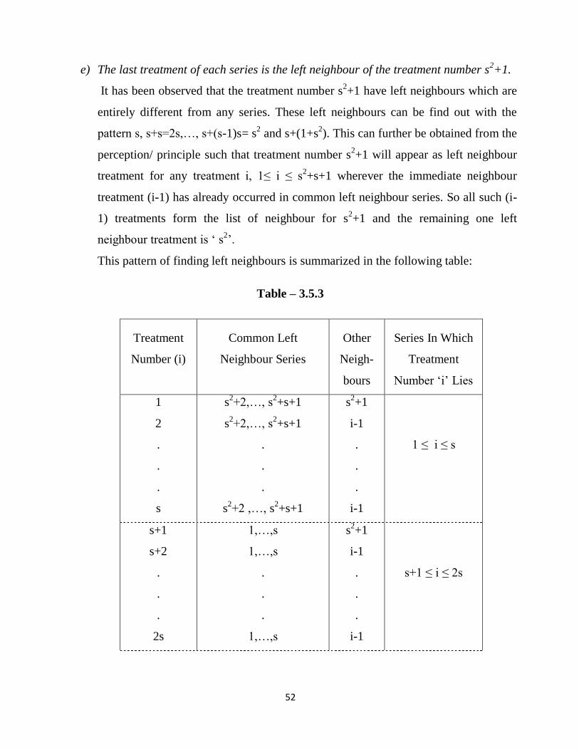
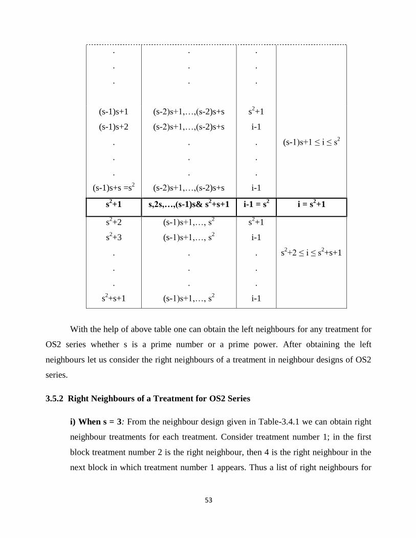
e) The last treatment of each series is the left neighbour of the treatment number s2+1.
It has been observed that the treatment number s2+1 have left neighbours which are
entirely different from any series. These left neighbours can be find out with the
pattern s, s+s=2s,…, s+(s-1)s= s2 and s+(1+s
2). This can further be obtained from the
perception/ principle such that treatment number s2+1 will appear as left neighbour
treatment for any treatment i, 1≤ i ≤ s2+s+1 wherever the immediate neighbour
treatment (i-1) has already occurred in common left neighbour series. So all such (i-
1) treatments form the list of neighbour for s2+1 and the remaining one left
neighbour treatment is ‘ s2’.
This pattern of finding left neighbours is summarized in the following table:
Table – 3.5.3
Treatment
Number (i)
Common Left
Neighbour Series
Other
Neigh-
bours
Series In Which
Treatment
Number ‘i’ Lies
1
2
.
.
.
s
s2+2,…, s
2+s+1
s2+2,…, s
2+s+1
.
.
.
s2+2 ,…, s
2+s+1
s2+1
i-1
.
.
.
i-1
1 ≤ i ≤ s
s+1
s+2
.
.
.
2s
1,…,s
1,…,s
.
.
.
1,…,s
s2+1
i-1
.
.
.
i-1
s+1 ≤ i ≤ 2s
53
.
.
.
.
.
.
.
.
.
(s-1)s+1
(s-1)s+2
.
.
.
(s-1)s+s =s2
(s-2)s+1,…,(s-2)s+s
(s-2)s+1,…,(s-2)s+s
.
.
.
(s-2)s+1,…,(s-2)s+s
s2+1
i-1
.
.
.
i-1
(s-1)s+1 ≤ i ≤ s2
s2+1 s,2s,…,(s-1)s& s
2+s+1 i-1 = s
2 i = s
2+1
s2+2
s2+3
.
.
.
s2+s+1
(s-1)s+1,…, s2
(s-1)s+1,…, s2
.
.
.
(s-1)s+1,…, s2
s2+1
i-1
.
.
.
i-1
s2+2 ≤ i ≤ s
2+s+1
With the help of above table one can obtain the left neighbours for any treatment for
OS2 series whether s is a prime number or a prime power. After obtaining the left
neighbours let us consider the right neighbours of a treatment in neighbour designs of OS2
series.
3.5.2 Right Neighbours of a Treatment for OS2 Series
i) When s = 3: From the neighbour design given in Table-3.4.1 we can obtain right
neighbour treatments for each treatment. Consider treatment number 1; in the first
block treatment number 2 is the right neighbour, then 4 is the right neighbour in the
next block in which treatment number 1 appears. Thus a list of right neighbours for
54
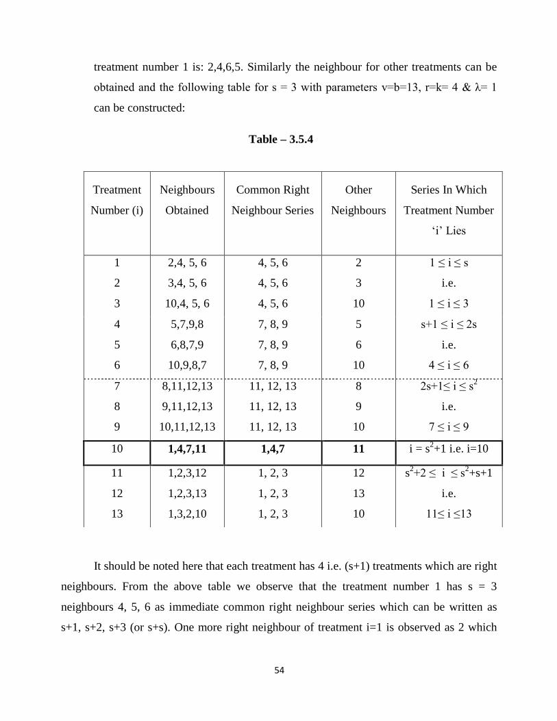
treatment number 1 is: 2,4,6,5. Similarly the neighbour for other treatments can be
obtained and the following table for s = 3 with parameters v=b=13, r=k= 4 & λ= 1
can be constructed:
Table – 3.5.4
It should be noted here that each treatment has 4 i.e. (s+1) treatments which are right
neighbours. From the above table we observe that the treatment number 1 has s = 3
neighbours 4, 5, 6 as immediate common right neighbour series which can be written as
s+1, s+2, s+3 (or s+s). One more right neighbour of treatment i=1 is observed as 2 which
Treatment
Number (i)
Neighbours
Obtained
Common Right
Neighbour Series
Other
Neighbours
Series In Which
Treatment Number
‘i’ Lies
1
2
3
2,4, 5, 6
3,4, 5, 6
10,4, 5, 6
4, 5, 6
4, 5, 6
4, 5, 6
2
3
10
1 ≤ i ≤ s
i.e.
1 ≤ i ≤ 3
4
5
6
5,7,9,8
6,8,7,9
10,9,8,7
7, 8, 9
7, 8, 9
7, 8, 9
5
6
10
s+1 ≤ i ≤ 2s
i.e.
4 ≤ i ≤ 6
7
8
9
8,11,12,13
9,11,12,13
10,11,12,13
11, 12, 13
11, 12, 13
11, 12, 13
8
9
10
2s+1≤ i ≤ s2
i.e.
7 ≤ i ≤ 9
10 1,4,7,11 1,4,7 11 i = s2+1 i.e. i=10
11
12
13
1,2,3,12
1,2,3,13
1,3,2,10
1, 2, 3
1, 2, 3
1, 2, 3
12
13
10
s2+2 ≤ i ≤ s
2+s+1
i.e.
11≤ i ≤13
55
can be written as i+1 for treatment number ‘i’ since the concept of right neighbour means
i+1.
The treatment number 2 has s = 3 neighbours 4,5,6 which is again immediate
common right neighbour series of i-th treatment (1 ≤ i ≤ s) which further can be written as
s+1, s+2, s+3 (or 2s). As noticed earlier, there shall be 4 right neighbours for each
treatment, so one more right neighbour of treatment number i=2 observed is 3 which may
be written as i+1 again.
Treatment number 3 has s = 3 neighbours 4,5,6 as the immediate common right
neighbour series of i-th treatment (1 ≤ i ≤ s) which further can be written as s+1, s+2, s+3
(or 2s). Here i+1 = 4 has already occurred as one of the members in the right common
series. So the repeated treatment number is replaced by the treatment number 10 or
treatment number s2+1. The logic of replacement of the repeated treatment by treatment
number s2+1 has been observed by Laxmi and Parmita for finding the pattern of left
neighbours in Neighbour Designs obtained from OS2 series. The right common series of ‘s’
treatments is immediately next series of the series in which treatment number ‘i’ lies,
assuming the treatment in circular way. So it may be percepted that one right neighbour of
i-th treatment is i+1. If this occurs in already obtained ‘s’ immediate common right
neighbours of the i-th treatment, it may be replaced by the treatment number s2+1.
The treatment number 4 or i = s+1 has s = 3 neighbours 7, 8, 9 which is immediate
common right neighbour series of the i-th treatment (s+1 ≤ i ≤ 2s). The right neighbours 7,
8, 9 can be written as 2s+1, 2s+2, 2s+s or s2. The one more right neighbour treatment of
treatment number i=4 is 5, which is written as i+1.
Now consider treatment number 5 or i =s+2 has s = 3 neighbours 7, 8, 9 which is
immediate common right neighbour series of the i-th treatment (s+1 ≤ i ≤ 2s). Here again
these can be written as 2s+1, 2s+2, 2s+s or s2. The one more right neighbour treatment of
treatment number i=5 is 6 which can be written as i+1.

56
Let us consider treatment number 6 or i =2s has s = 3 neighbours 7, 8, 9 which is
immediate common right neighbour series of the i-th treatment (s+1 ≤ i ≤ 2s). The one
more right neighbour treatment of treatment number i=6 is observed as 10. According to
the perception this should be i+1 i.e. 7. But treatment number 7 has already occurred as one
of the members in the right series. Now it is replaced by the treatment number 10 i.e. s2+1.
The treatment number 7 or i =2s+1 has s = 3 neighbours 11,12,13 as the immediate
common right neighbour series of the i-th treatment (2s+1 ≤ i ≤ 3s or s2). Now the right
neighbours 11,12,13 can be written as s2+2, s
2+3 or s
2+s, s
2+s+1. The one more right
neighbour treatment of treatment number i=7 is 8 which is written as i+1.
Consider the treatment number 8 or i =2s+2 has s = 3 neighbours 11,12,13 which is
immediate common right neighbour series of the i-th treatment (2s+1 ≤ i ≤ 3s or s2). The
one more right neighbour treatment of treatment number i=8 is observed as 9 which is
written as i+1.
Now the treatment number 9 or i = s2 has s = 3 neighbours 11,12,13 which is
immediate common right neighbour series of the i-th treatment (2s+1 ≤ i ≤ 3s or s2). The
one more right neighbour treatment of treatment number i=9 is 10 which is written as i+1.
We observed that treatment number 10 or i = s2+1 has neighbours which are entirely
different from the series and the conception, so we shall discuss it later.
Consider the treatment number 11 or i = s2+2. The immediate common right
neighbour series of the i-th treatment (s2+2 ≤ i ≤ s
2+s+1) should be s
2+s+2, s
2+s+3, s
2+s+s,
s2+2s+1. These right neighbours with mod(v) can be written as 1,…,s. So the right common
neighbour series is 1,2,3. The one more right neighbour treatment of treatment number i=11
is observed as 12 which is written as i+1. As observed treatment number s2+1=10 is a
treatment which has entirely different neighbour treatments and also does not occur in
immediate common right neighbour series of any treatment.
57
The treatment number 12 or i = s2+s has s = 3 neighbours 1, 2, 3 which is immediate
common right neighbour series of the i-th treatment (s2+2 ≤ i ≤ s
2+s+1). The one more
right neighbour treatment of treatment number i=12 is observed as 13 which is written as
i+1.
The treatment number 13 or i = s2+s+1 has s = 3 neighbours 1, 2, 3 which is
immediate common right neighbour series of the i-th treatment (s2+2 ≤ i ≤ s
2+s+1). The
one more right neighbour treatment of treatment number i=13 can be observed as
14(mod13) = 1 which is written as i+1. But treatment number 1 has already occurred as one
of the members in immediate common right neighbour series. So it is replaced by the
treatment number 10 i.e. s2+1.
As observed treatment number s2+1=10 is a treatment which has entirely different
neighbour treatments. It is to be noted here that treatment number 10 does not occur in the
right series of any treatment. The treatment number 10 or i = s2+1 has right neighbours
1,4,7 and 11. These neighbours can be written as 1, s+1, 2s+1 and s2+2. This shows that the
first treatment of all the series are the right neighbour of the treatment number 10 i.e. first
treatment of series 1 ≤ i ≤ s, s+1 ≤ i ≤ 2s, 2s+1 ≤ i ≤ s2,s
2+2 ≤ i ≤ s
2+s+1.
This can further be interpreted from the perception/ principle that treatment number
s2+1 will appear as neighbour treatment for the treatment i, 1≤ i ≤ s
2+s+1 wherever the
immediate right neighbour treatment (i+1) has already occurred in the immediate common
right series. So all such (i+1) treatments forms the list of neighbours for s2+1 and the
remaining one right neighbour treatment is the immediate right neighbour i.e. ‘s2+2’.
iii) When s = 4: For s = 4 i.e. when s is a prime power, the neighbour design so obtained
is given in Table-3.4.2 from which we observed right neighbour treatments of each
treatment. Consider the treatment number 1; in the first block it has 2 as the right
neighbour, then 5 is the right neighbour in the next block in which treatment number
1 appears. Similarly, we get neighbours from the other blocks in which treatment
number 1 appears. Thus a list of neighbours for treatment number 1 is: 2,5,6,8,7.
58
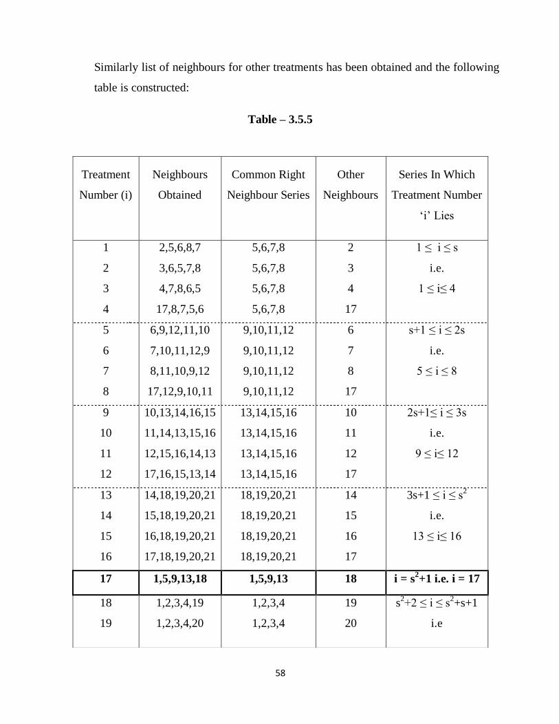
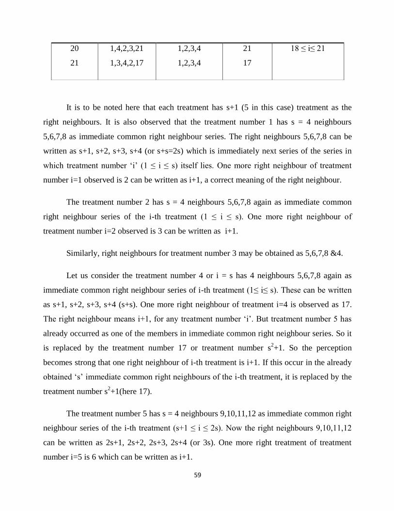
Similarly list of neighbours for other treatments has been obtained and the following
table is constructed:
Table – 3.5.5
Treatment
Number (i)
Neighbours
Obtained
Common Right
Neighbour Series
Other
Neighbours
Series In Which
Treatment Number
‘i’ Lies
1
2
3
4
2,5,6,8,7
3,6,5,7,8
4,7,8,6,5
17,8,7,5,6
5,6,7,8
5,6,7,8
5,6,7,8
5,6,7,8
2
3
4
17
1 ≤ i ≤ s
i.e.
1 ≤ i≤ 4
5
6
7
8
6,9,12,11,10
7,10,11,12,9
8,11,10,9,12
17,12,9,10,11
9,10,11,12
9,10,11,12
9,10,11,12
9,10,11,12
6
7
8
17
s+1 ≤ i ≤ 2s
i.e.
5 ≤ i ≤ 8
9
10
11
12
10,13,14,16,15
11,14,13,15,16
12,15,16,14,13
17,16,15,13,14
13,14,15,16
13,14,15,16
13,14,15,16
13,14,15,16
10
11
12
17
2s+1≤ i ≤ 3s
i.e.
9 ≤ i≤ 12
13
14
15
16
14,18,19,20,21
15,18,19,20,21
16,18,19,20,21
17,18,19,20,21
18,19,20,21
18,19,20,21
18,19,20,21
18,19,20,21
14
15
16
17
3s+1 ≤ i ≤ s2
i.e.
13 ≤ i≤ 16
17 1,5,9,13,18 1,5,9,13 18 i = s2+1 i.e. i = 17
18
19
1,2,3,4,19
1,2,3,4,20
1,2,3,4
1,2,3,4
19
20
s2+2 ≤ i ≤ s
2+s+1
i.e
59
It is to be noted here that each treatment has s+1 (5 in this case) treatment as the
right neighbours. It is also observed that the treatment number 1 has s = 4 neighbours
5,6,7,8 as immediate common right neighbour series. The right neighbours 5,6,7,8 can be
written as s+1, s+2, s+3, s+4 (or s+s=2s) which is immediately next series of the series in
which treatment number ‘i’ (1 ≤ i ≤ s) itself lies. One more right neighbour of treatment
number i=1 observed is 2 can be written as i+1, a correct meaning of the right neighbour.
The treatment number 2 has s = 4 neighbours 5,6,7,8 again as immediate common
right neighbour series of the i-th treatment (1 ≤ i ≤ s). One more right neighbour of
treatment number i=2 observed is 3 can be written as i+1.
Similarly, right neighbours for treatment number 3 may be obtained as 5,6,7,8 &4.
Let us consider the treatment number 4 or i = s has 4 neighbours 5,6,7,8 again as
immediate common right neighbour series of i-th treatment (1≤ i≤ s). These can be written
as s+1, s+2, s+3, s+4 (s+s). One more right neighbour of treatment i=4 is observed as 17.
The right neighbour means i+1, for any treatment number ‘i’. But treatment number 5 has
already occurred as one of the members in immediate common right neighbour series. So it
is replaced by the treatment number 17 or treatment number s2+1. So the perception
becomes strong that one right neighbour of i-th treatment is i+1. If this occur in the already
obtained ‘s’ immediate common right neighbours of the i-th treatment, it is replaced by the
treatment number s2+1(here 17).
The treatment number 5 has s = 4 neighbours 9,10,11,12 as immediate common right
neighbour series of the i-th treatment (s+1 ≤ i ≤ 2s). Now the right neighbours 9,10,11,12
can be written as 2s+1, 2s+2, 2s+3, 2s+4 (or 3s). One more right treatment of treatment
number i=5 is 6 which can be written as i+1.
20
21
1,4,2,3,21
1,3,4,2,17
1,2,3,4
1,2,3,4
21
17
18 ≤ i≤ 21
60
Now consider the treatment number 6 or i= s+2 has s = 4 neighbours 9,10,11,12 as
immediate common right neighbour series of the i-th treatment (s+1 ≤ i ≤ 2s). One more
right treatment of treatment number i=6 is 7 which can be written as i+1 as it should be.
Using the same pattern, neighbours for the treatment number 7 is 9,10,11,12 & 8.
Consider the treatment number 8 or i= 2s has s = 4 neighbours 9,10,11,12 as
immediate common right neighbour series of the i-th treatment (s+1 ≤ i ≤ 2s). One more
right neighbour treatment of treatment number i=8 observed is 17. According to the
perception it should be i+1 i.e. 9. As the treatment number 9 has already occurred as one of
the members in immediate common right neighbour series, so it should be replaced by the
treatment number s2+1=17, which shows that the perception is true.
In the same way, neighbours for the treatment numbers 9, 10 and 11 are 13,14,15,16
& 10; 13,14,15,16 & 11 and 13,14,15,16 & 12 respectively.
Now consider the treatment number 12 or i= 3s has the same 4 neighbours
13,14,15,16 as immediate common right neighbour series of the i-th treatment (2s+1 ≤ i ≤
3s). One more right treatment of treatment number i=12 observed is 17. It should be
according to the perception i+1 i.e. 13. As the treatment number 13 has already occurred as
one of the members in immediate common right series. So it is replaced by the treatment
number s2+1=17 which again shows that our perception is true.
The treatment number 13 or i= 3s+1 has s = 4 neighbours 18,19,20,21 as immediate
common right neighbour series of i-th treatment (3s+1 ≤ i ≤ s2). These right treatments
18,19,20,21 can be written as s2+2, s
2+3, s
2+4 (or s
2+s), s
2+5 (or s
2+s+1). One more right
neighbour of treatment number i=13 observed is 14 which can be written as i+1.
Similarly, the right neighbour treatments for the treatment number 14 and 15 i.e.
i=14,15 are observed as 18,19,20,21 & 15 and 18,19,20,21 & 16 respectively.
61
Consider the treatment number 16 or i= s2 (here) has the same 4 neighbours
18,19,20,21 as immediate common right neighbour series of the i-th treatment (3s+1 ≤ i ≤
s2). One more right neighbour treatment of treatment number i=16 observed is 17 which
can be written as i+1.
When s = 3, a prime number, we observed that treatment number s2+1 = 10 has a
different list of neighbours. Similarly, when s = 4, a prime power, we observed that
treatment number 17 i.e. ‘s2+1’ has neighbours which are entirely different from the series
and the conception, so we shall discuss it later.
Consider the treatment number 18 or i= s2+2. The immediate common right
neighbour series of the i-th treatment (s2+2 ≤ i ≤ s
2+s+1) should be s
2+s+2, s
2+s+3, s
2+s+s,
s2+2s+1. These right neighbours with mod(v) can be written as 1,…,s. So the common right
neighbour series is 1,2,3,4. One more right neighbour of treatment number i=18 observed is
19 which can be written as i+1. As observed treatment number s2+1=17 is a treatment
which has entirely different neighbour treatments and also does not occur in immediate
common right neighbour series of any treatment.
In the same way, the neighbours for the treatment number 19 and 20 are 1,2,3,4 &
20 and 1,2,3,4 & 21 respectively.
The treatment number 21 or i= s2+s+1 has 4 neighbours 1,2,3,4 as immediate
common right neighbour series of the i-th treatment (s2+2 ≤ i ≤ s
2+s+1). One more right
neighbour of treatment number i=21 should be according to the perception i+1 i.e. 22(mod
21)=1. But the treatment number 1 has already occurred as one of the members in
immediate common right neighbour series. So it is replaced by the treatment number
s2+1=17 which again proves that our perception is true.
The treatment number 17 or i= s2+1 has the neighbours 1,5,9,13,18. These
neighbours can be written as 1, s+1, 2s+1, 3s+1, and s2+2s. This shows that the first
62
treatment of all the series i.e. 1 ≤ i ≤ s, s+1 ≤ i ≤ 2s, 2s+1≤ i ≤ 3s, 3s+1 ≤ i ≤ s2, s
2+2 ≤ i ≤
s2+s+1 are the right neighbours of the treatment number 17.
This can further be interpreted from the perception/ principle that the treatment
number s2+1 will appear as neighbour treatment for the treatment i, 1≤ i ≤ s
2+s+1 wherever
the neighbour treatment (i+1) has already occurred in immediate common right neighbour
series. So all such (i+1) treatments forms the list of right neighbours for treatment number
s2+1 and the remaining one right neighbour treatment is immediate right neighbour i.e.
‘s2+2’.
i) Steps to find Right Neighbours
a) Observe the treatment number ‘i’, where i ≠ s2+1.
b) Then find the series in which the treatment number ‘i’ lies.
The series is defined in such a way that the sequence of first ‘s’ treatments of the
design forms the first series, the sequence of next ‘s’ treatments i.e. ‘s+1’ to ‘2s’
forms the second series and so on upto ‘s2’. Thus have ‘s’ series upto the treatment
number ‘s2’. The last series i.e. ‘s+1’–th series of ‘s’ treatments always starts from
treatment number ‘s2+2’ instead of the treatment number ‘s
2+1’ and ended on
treatment number ‘s2+s+1’ for any ‘s’ whether it is a prime number or prime power.
It is due to the reason that whenever an immediate right-neighbour of i-th treatment
i.e. i+1 occurs already in the immediate common right neighbour series then that
repeated treatment is replaced by the treatment number ‘s2+1’. Further ‘s+2’-th
series of next ‘s’ treatments shall be ‘s2+s+2’ to ‘s
2+2s+1’, which with mod(v)
reduces to ‘1’ to ‘s’. So the s+2-th series is again the first series of the design. This
again holds that the design is circular.
c) Then find out the immediate common right neighbour series for that treatment.
Let the treatment number ‘i’ lies in the j-th series (j=1,2,…,s+1), then ‘j+1’-th series
is the next series or immediate common right neighbour series.
63
d) One more right neighbour treatment can be find by the concept of right neighbour
that means right adjacent.
This should be i+1 for the treatment number ‘i’. If this right treatment already occurs
in the immediate common right neighbour series then that ‘i+1’–th treatment is
replaced by the treatment number s2+1.
e) The first treatment of each series is the right neighbour of the treatment number
s2+1.
It has been observed that the treatment number s2+1 has right neighbours which are
entirely different from any series. These right neighbours can be find out with the
pattern 1, s+1, 2s+1, … , (s-1)s+1 and (1+s2)+1 i.e.s
2+2. This can further be
interpreted from the perception/ principle that treatment number s2+1 will appear as
right neighbour treatment for any treatment i, 1≤ i ≤ s2+s+1 wherever the immediate
neighbour treatment (i+1) has already occurred in immediate common right
neighbour series. So all such (i+1) treatments form the list of neighbour for s2+1 and
the remaining one right neighbour treatment is immediate right neighbour is ‘s2+2’.
For neighbour designs with parameters v=b=s2+s+1, r=k=s+1 & λ=1, it should be noted
that there shall always be s+1 treatments for each treatment as the right neighbours. This
pattern of finding right neighbours is summarized in the following table:

64
Table-3.5.6
Series In Which
Treatment
Number ‘i’ Lies
Treatment
Number (i)
Common Right
Neighbour Series
Other Right
Neighbour
1 ≤ i ≤ s
1
2
.
.
.
s
s+1,…,2s
s+1,…,2s
.
.
.
s+1,…,2s
i+1
i+1
.
.
.
s2+1
s+1 ≤ i ≤ 2s
s+1
s+2
.
.
.
2s
2s+1,…,3s
2s+1,…,3s
.
.
.
2s+1,…,3s
i+1
i+1
.
.
.
s2+1
.
.
.
.
.
.
.
.
.
(s-1)s+1 ≤ i ≤ s2
(s-1)s+1
(s-1)s+2
.
.
s2+2 ,…, s
2+s+1
s2+2 ,…, s
2+s+1
.
.
i+1
i+1
.
.
65
.
(s-1)s+s =s2
.
s2+2 ,…, s
2+s+1
.
i+1= s2+1
i = s2+1 s
2+1 1,s+1,2s+1,…,(s-
1)s+1
i+1=s2+2
s2+2 ≤ i ≤ s
2+s+1
s2+2
s2+3
.
.
.
s2+s+1
1,…,s
1,…,s
.
.
.
1,…,s
i+1
i+1
.
.
.
s2+1
With the help of above table one can obtain the right neighbours for any treatment
for OS2 series whether s is a prime number or a prime power.
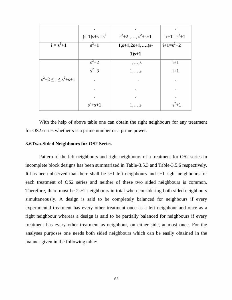
3.6Two-Sided Neighbours for OS2 Series
Pattern of the left neighbours and right neighbours of a treatment for OS2 series in
incomplete block designs has been summarized in Table-3.5.3 and Table-3.5.6 respectively.
It has been observed that there shall be s+1 left neighbours and s+1 right neighbours for
each treatment of OS2 series and neither of these two sided neighbours is common.
Therefore, there must be 2s+2 neighbours in total when considering both sided neighbours
simultaneously. A design is said to be completely balanced for neighbours if every
experimental treatment has every other treatment once as a left neighbour and once as a
right neighbour whereas a design is said to be partially balanced for neighbours if every
treatment has every other treatment as neighbour, on either side, at most once. For the
analyses purposes one needs both sided neighbours which can be easily obtained in the
manner given in the following table:
66
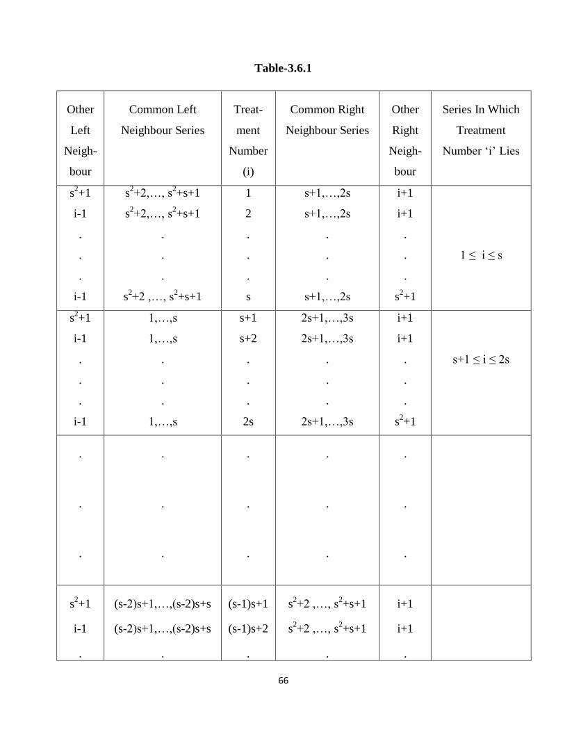
Table-3.6.1
Other
Left
Neigh-
bour
Common Left
Neighbour Series
Treat-
ment
Number
(i)
Common Right
Neighbour Series
Other
Right
Neigh-
bour
Series In Which
Treatment
Number ‘i’ Lies
s2+1
i-1
.
.
.
i-1
s2+2,…, s
2+s+1
s2+2,…, s
2+s+1
.
.
.
s2+2 ,…, s
2+s+1
1
2
.
.
.
s
s+1,…,2s
s+1,…,2s
.
.
.
s+1,…,2s
i+1
i+1
.
.
.
s2+1
1 ≤ i ≤ s
s2+1
i-1
.
.
.
i-1
1,…,s
1,…,s
.
.
.
1,…,s
s+1
s+2
.
.
.
2s
2s+1,…,3s
2s+1,…,3s
.
.
.
2s+1,…,3s
i+1
i+1
.
.
.
s2+1
s+1 ≤ i ≤ 2s
.
.
.
.
.
.
.
.
.
.
.
.
.
.
.
s2+1
i-1
.
(s-2)s+1,…,(s-2)s+s
(s-2)s+1,…,(s-2)s+s
.
(s-1)s+1
(s-1)s+2
.
s2+2 ,…, s
2+s+1
s2+2 ,…, s
2+s+1
.
i+1
i+1
.
67
.
.
i-1
.
.
(s-2)s+1,…,(s-2)s+s
.
.
(s-1)s+s
=s2
.
.
s2+2 ,…, s
2+s+1
.
.
i+1=
s2+1
(s-1)s+1 ≤ i ≤ s2
i-1 = s2 s,2s,…,(s-1)s&
s2+s+1
s2+1 1,s+1,2s+1,…, (s-
1)s+1
i+1=
s2+2
i = s2+1
s2+1
i-1
.
.
.
i-1
(s-1)s+1,…, s2
(s-1)s+1,…, s2
.
.
.
(s-1)s+1,…, s2
s2+2
s2+3
.
.
.
s2+s+1
1,…,s
1,…,s
.
.
.
1,…,s
i+1
i+1
.
.
.
s2+1
s2+2 ≤ i ≤ s
2+s+1
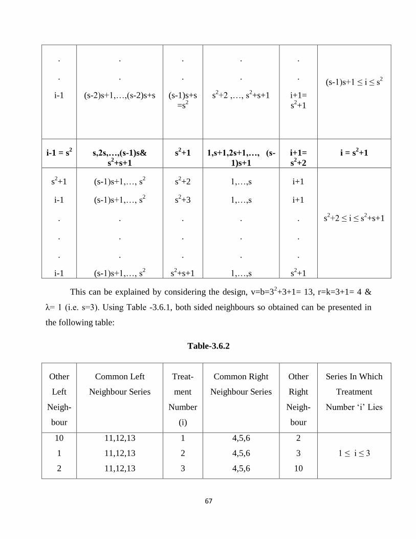
This can be explained by considering the design, v=b=32+3+1= 13, r=k=3+1= 4 &
λ= 1 (i.e. s=3). Using Table -3.6.1, both sided neighbours so obtained can be presented in
the following table:
Table-3.6.2
Other
Left
Neigh-
bour
Common Left
Neighbour Series
Treat-
ment
Number
(i)
Common Right
Neighbour Series
Other
Right
Neigh-
bour
Series In Which
Treatment
Number ‘i’ Lies
10
1
2
11,12,13
11,12,13
11,12,13
1
2
3
4,5,6
4,5,6
4,5,6
2
3
10
1 ≤ i ≤ 3

68
10
4
5
1,2,3
1,2,3
1,2,3
4
5
6
7,8,9
7,8,9
7,8,9
5
6
10
4≤ i ≤ 6
10
7
8
4,5,6
4,5,6
4,5,6
7
8
9
11,12,13
11,12,13
11,12,13
8
9
10
7≤ i ≤ 9
9 3,6,13 10 1,4,7 11 i = 10
10
11
12
7,8,9
7,8,9
7,8,9
11
12
13
1,2,3
1,2,3
1,2,3
12
13
10
11≤ i ≤ 13
From the above table we observe that the treatment number 1 has s = 3 neighbours
11,12,13 as common left neighbours which is the series immediate left to the series in
which i-th treatment (1 ≤ i ≤ s) lies. Other s = 3 neighbours are 4,5,6 as common right
neighbours which is the series immediate right to the series in which i-th treatment (1 ≤ i ≤
s) lies. Here the left neighbours 11, 12, 13 can be written as s2+2, s
2+3 (or s
2+s), s
2+4 (or
s2+s+1). Similarly 4, 5, 6 can be written as s+1, s+2, s+3 (or s+s/2s). Other two treatments
of i=1 are observed as 10, 2. As the concept of neighbour means adjacent it should be i-1
and i+1, where i+1=2 is the immediate right neighbour of i and i-1 =0(mod v) = 13 has
already occurred as one of the members in the left series, is replaced by the treatment
number 10 which can be written as treatment number s2+1. So it may be percepted that
other two neighbours of i-th treatment are i-1 and i+1. If any of these two occur in the
previously obtained 2s neighbours of the i-th treatment, it may be replaced by the treatment
number s2+1.
The treatment number 2 has s = 3 neighbours 11, 12, 13 which is again immediate
common left neighbour series which can be written as s2+2, s
2+3 (or s
2+s), s
2+4 (or s
2+s+1).
Other s = 3 neighbours are 4, 5, 6 which is again the immediate common right neighbour
series of i-th treatment (1 ≤ i ≤ s) which further can be written as s+1, s+2, s+3 (or 2s). As
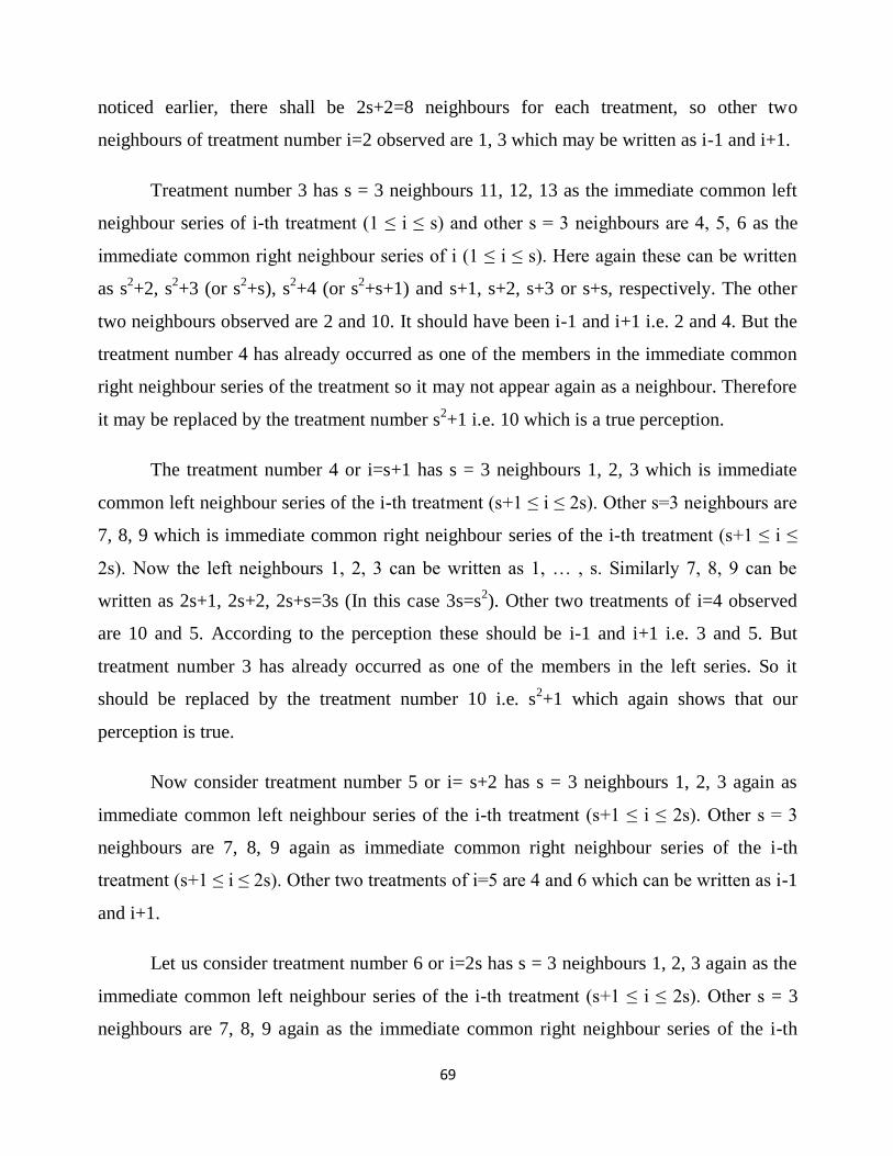
69
noticed earlier, there shall be 2s+2=8 neighbours for each treatment, so other two
neighbours of treatment number i=2 observed are 1, 3 which may be written as i-1 and i+1.
Treatment number 3 has s = 3 neighbours 11, 12, 13 as the immediate common left
neighbour series of i-th treatment (1 ≤ i ≤ s) and other s = 3 neighbours are 4, 5, 6 as the
immediate common right neighbour series of i (1 ≤ i ≤ s). Here again these can be written
as s2+2, s
2+3 (or s
2+s), s
2+4 (or s
2+s+1) and s+1, s+2, s+3 or s+s, respectively. The other
two neighbours observed are 2 and 10. It should have been i-1 and i+1 i.e. 2 and 4. But the
treatment number 4 has already occurred as one of the members in the immediate common
right neighbour series of the treatment so it may not appear again as a neighbour. Therefore
it may be replaced by the treatment number s2+1 i.e. 10 which is a true perception.
The treatment number 4 or i=s+1 has s = 3 neighbours 1, 2, 3 which is immediate
common left neighbour series of the i-th treatment (s+1 ≤ i ≤ 2s). Other s=3 neighbours are
7, 8, 9 which is immediate common right neighbour series of the i-th treatment (s+1 ≤ i ≤
2s). Now the left neighbours 1, 2, 3 can be written as 1, … , s. Similarly 7, 8, 9 can be
written as 2s+1, 2s+2, 2s+s=3s (In this case 3s=s2). Other two treatments of i=4 observed
are 10 and 5. According to the perception these should be i-1 and i+1 i.e. 3 and 5. But
treatment number 3 has already occurred as one of the members in the left series. So it
should be replaced by the treatment number 10 i.e. s2+1 which again shows that our
perception is true.
Now consider treatment number 5 or i= s+2 has s = 3 neighbours 1, 2, 3 again as
immediate common left neighbour series of the i-th treatment (s+1 ≤ i ≤ 2s). Other s = 3
neighbours are 7, 8, 9 again as immediate common right neighbour series of the i-th
treatment (s+1 ≤ i ≤ 2s). Other two treatments of i=5 are 4 and 6 which can be written as i-1
and i+1.
Let us consider treatment number 6 or i=2s has s = 3 neighbours 1, 2, 3 again as the
immediate common left neighbour series of the i-th treatment (s+1 ≤ i ≤ 2s). Other s = 3
neighbours are 7, 8, 9 again as the immediate common right neighbour series of the i-th
70
treatment (s+1 ≤ i ≤ 2s). Other two treatments of i=6 are 5 and 10. According to the
perception it should be i-1 and i+1 i.e. 5 and 7. As treatment number 7 has already occurred
as one of the members in the right series. So it is replaced by the treatment number
s2+1=10.
The treatment number 7 or i=2s+1 has s = 3 neighbours 4, 5, 6 as the immediate
common left neighbour series of thei-th treatment (2s+1 ≤ i ≤ 3s/s2). Other s = 3 neighbours
are 11, 12, 13 as the immediate common right neighbour series of the i-th treatment (2s+1 ≤
i ≤ 3s/s2). Now the left neighbours 4, 5, 6 can be written as s+1, s+2, s+s(=2s). Similarly 11,
12, 13 can be written as s2+2, s
2+3 (or s
2+s), s
2+4 (or s
2+s+1). The other two neighbours of
treatment number i=7 are 10 and 8. It should be according to the perception i-1 and i+1 i.e.
6 and 8. But treatment number 6 has already occurred as one of the members in the left
series. So it is replaced by the treatment number 10 i.e. s2+1. It is noted here that the
immediate common right neighbour series of the treatment number i (7≤ i ≤ 9) is s2+2,
s2+3, s
2+4 instead of s
2+1, s
2+2, s
2+3. It may be due to the reason that whenever an
immediate neighbour of i i.e. either i-1 or i+1 occurs in immediate common left neighbour
series or immediate common right neighbour series, it may be replaced by s2+1.
Consider the treatment number 8 or i=2s+2 has s = 3 neighbours 4, 5, 6 which is
immediate common left neighbour series of the i-th treatment (2s+1 ≤ i ≤ 3s/s2). Other s = 3
neighbours are 11, 12, 13 which is immediate common right neighbour series of the i-th
treatment (2s+1 ≤ i ≤ 3s/s2). Other two neighbours of treatment number i=8 observed are 7
and 9. These two neighbour treatments can be further written as i-1 and i+1.
Now the treatment number 9 or i=s2 has s = 3 neighbours 4, 5, 6 which is immediate
common left neighbour series of the i-th treatment (2s+1 ≤ i ≤ 3s/s2). Other s=3 neighbours
are 11, 12, 13 which is immediate common right neighbour series of the i-th treatment
(2s+1 ≤ i ≤ 3s/s2). The other two neighbours of treatment number i=9 are 8 and 10 which is
written as i-1 and i+1.
71
We observed that treatment 10 i.e. s2+1 has neighbours which are entirely different
from the series and the conception, so we will discuss it later.
Let us consider the treatment number 11or i=s2+2 has s = 3 neighbours 7, 8, 9 which
is immediate common left neighbour series of the i-th treatment (s2+2 ≤ i ≤ s
2+s+1). Other s
= 3 neighbours are 1, 2, 3 which is immediate common right neighbour series of the i-th
treatment (s2+2 ≤ i ≤ s
2+s+1). The left neighbours 7, 8, 9 can be written as 2s+1, 2s+2, 2s+s
or s2. Similarly right neighbours can be written as s
2+s+2 (mod 13) =1, s
2+s+3 (mod 13) =2,
s2+2s+1 (mod 13) = 3 or s. Other two neighbours of treatment number i=11 observed are 10
and 12 which can be written as i-1 and i+1. As observed treatment number s2+1=10 is a
treatment which has entirely different neighbour treatments. It is also observed here that
treatment number s2+1=10 does not occur in the immediate common left neighbour series
or right neighbour series of any treatment.
The treatment number 12 or i=s2+s has s = 3 neighbours 7, 8, 9 which is immediate
common left neighbour series of the i-th treatment (s2+2 ≤ i ≤ s
2+s+1). Other s = 3
neighbours are 1, 2, 3 which is immediate common right neighbour series of the i-th
treatment. Other two neighbours of treatment number i=12 observed are 11 and 13 which
can be written as i-1 and i+1.
The treatment number 13 or i=s2+s+1 has s = 3 neighbours 7, 8, 9 which is
immediate common left neighbour series of the i-th treatment (s2+2 ≤ i ≤ s
2+s+1). Other s =
3 neighbours are 1, 2, 3 which is immediate common right neighbour series of the i-th
treatment (s2+2 ≤ i ≤ s
2+s+1). The other two neighbours of treatment number i=13 observed
are 12 and 10 which should be according to the perception (i-1 and i+1) i.e. 12 and
14(mod13) = 1. But treatment number 1 has already occurred as one of the members in the
right series. So it is replaced by the treatment number 10 i.e. s2+1.
As observed treatment number s2+1=10 is a treatment which has entirely different
neighbour treatments. The treatment number 10 or i=s2+1 has the neighbours 1, 3, 4, 6, 7, 9,
11 & 13. These neighbours can be written as 1, s, s+1, s+s/(2s), 2s+1, 2s+s/(3s=s2)
in this
72
case), s2+2 and s
2+s+1. This shows that the first treatment and the last treatment of all the
series are the neighbours of the treatment number 10 or s2+1.
This can further be observed from the perception such that treatment number s2+1
will appear as neighbour treatment for any treatment i, 1≤ i ≤ s2+s+1wherever the
immediate neighbour treatments (i-1, i+1)has already occurred in either left series or right
series. So all such treatments come in the list of neighbour for s2+1 and the rest two
neighbour treatments are immediate neighbour of treatment number s2+1 i.e. s
2 and s
2+2.
This procedure of finding the neighbours is same for any value of s, whether s is a prime
number or a prime power. Here it should be noted that every treatment does not have every
other treatment as its neighbours, so it is incompletely balanced for neighbours for OS2
series as there shall be only 2s+2 neighbours of a treatment when considering both sides
simultaneously. These neighbours can be obtained in the following steps.
i) Steps To Find Two-Sided Neighbours For OS2 Series
a) Observe the treatment number ‘i’, where i ≠ s2+1.
b) Then find the series in which the treatment number ‘i’ lies.
The series is defined in such a way that the sequence of first ‘s’ treatments of the
design form the first series, the sequence of next ‘s’ treatments i.e. ‘s+1’ to ‘2s’ form
the second series and so on up to ‘s2’. Thus have ‘s’ series up to the treatment
number ‘s2’. The last series i.e. ‘s+1’–th series of ‘s’ treatments always starts from
treatment number ‘s2+2’ instead of the treatment number ‘s
2+1’ and ended on
treatment number ‘s2+s+1’ for any ‘s’ whether it is a prime number or prime power.
Now the ‘s+2’-th series of next ‘s’ treatments shall be ‘s2+s+2’ to ‘s
2+2s+1’, which
with mod(v) reduces to ‘1’ to ‘s’. So the s+2-th series is again the first series of the
design. This shows that the design is circular.
c) Then find out the immediate common left neighbour series and immediate
common right neighbour series for the treatment.

73
d) Other two neighbour treatments i.e. left neighbour and right neighbour can be
find by taking left adjacent and right adjacent of the treatment respectively.
e) The last and first treatments of each series are respectively the left and right
neighbours of the treatment number s2+1.
Now we can obtain left and right neighbours for any treatment for the neighbour
design of OS2 series, using the above discussed short-cut method. Then the statistical
analysis of neighbour treatments and stability measures will become convenient and that
will be discussed in later chapters.
(This pattern of finding two-sided neighbours has been observed only for OS2 series
of BIBD. It may work for other designs also).
References
Eberhart, S.A. and Russel, W.A. (1966). Stability parameters for comparing varieties. Crop
Sci., 6, 36-40.
Finlay, K.W. and Wilkinson, G.N. (1963).The analysis of adaptation in a plant breeding
programme. Aust. J. Agri. Res., 14, 742-754.
Fisher, R.A. (1935): The Design of Experiments. Edinburgh: Oliver and Boyd.
Freeman, G.H. and Perkins, J.M. (1971): Environmental and genotype-environmental
components of variability VIII. Relation between genotype grown in different
environments and measurement of these environments. Heredity, 27, 15-23.
Laxmi, R.R.,(1992): Genotype-Environment interaction: Its role in stability of crop
varieties. Unpublished thesis, submitted to IASRI, New Delhi.
Laxmi, Ratna Raj and Gupta, Renu (2000): Different approaches for stability measures in

74
relation to genotype-environment interaction. Crop Research,20(1), 118-125.
Perkins, J. M. and Jinks, J. L. (1968).Environmental and genotype environmental
components of variability, III. Multiple lines and crosses. Heredity, 23, 339-356.
Perkins, J. M. and Jinks, J. L. (1968).Environmental and GE components of variability,
IV.Non-linear interactions for multiple inbred lines.Heredity, 23, 525-535.
Rees, D. H. (1967): Some designs of use in serology. Biometrics, 23, 779-791.
Shukla, G.K. (1972a). Some statistical aspects of partitioning genotype-environmental
components of variability. Heredity, 29, 237-245.
Yates, F. (1936). Incomplete randomized blocks. Ann. Eugen.,7, 121-140
Yates, F. and Cochran, W.G. (1938): The analysis of group of experiments. J. Agric. Sci.,
Camb., 28, 556-580.