Embed Size (px)
Citation preview

CHAPTER –II
QUANTUM CHEMICAL CALCULATIONS AND
NORMAL COORDINATE ANALYSIS
Abstract
The different stages involved in quantum chemical
calculations are discussed. An overview of density functional
theory and the different types of basis sets are outlined. The
various stages involved in normal coordinate analysis of
polyatomic molecules are described. The procedure of performing
Scaled quantum chemical calculations using MOLVIB software is
explained.

CHAPTER –II
QUANTUM CHEMICAL CALCULATIONS AND NORMAL
COORDINATE ANALYSIS
2.1 INTRODUCTION
The philosophy of computational methods of vibrational spectroscopy
[68-69, 24] changed significantly when quantum mechanical programmes for
optimization of the geometry of a molecule and for analytical determination of
its force field appeared. Harmonic force fields derived from quantum
mechanics are widely used at present for the calculation of frequencies and
the modes of normal vibrations.
Indeed, applying current quantum-mechanical methods has made it
possible to replace the parameters mentioned above by their more clearly
defined quantum-mechanical analogues in the theory of small-amplitude
vibrations. This opened the way to calculating the frequencies and intensities
of spectral bands with a minimum degree of arbitrariness (although the
degree depends on the level of the quantum-mechanical treatment) and
finding rational explanations for a number of chemical and physical properties
of substances.
However, in numerous current quantum-mechanical calculations
vibrational spectra performed at different levels of approximation, calculated
frequencies are, as a rule, higher than their experimental counterparts. This
outcome is due to the more or less systematic overestimation of the force
constants in the Hartree-Fock method [70]. This overestimation of the force
constants depends on the basis set employed [71] and to the not-so-regular
discrepancies in applications of the Moller-Plesset theory [72]. These

calculations required empirical corrections. To improve agreement with
experiment, quantum-mechanical force fields are corrected in one way or
another, e.g. using empirical corrections called scale factors, which are
estimated from the experimental vibrational spectra of small molecules with
reliable frequency assignments.
Second-order Moller-Plesset perturbation theory (MP2) cannot fully
take the correlation energy of a system into account (the more so when
restricted basis sets are used). Thus, using this theory does not obviate the
necessity of scaling force constants. Moreover, with some molecules
containing heteroatoms [73], especially halogens [74, 75], this approximation
leads to irregular deviations of calculated frequencies from experiment.
Nowadays sophisticated electron correlation calculations are
increasingly available and deliver force fields of high accuracy for small
polyatomics. The scaled quantum mechanical force fields [76] are of
comparable accuracy with the best purely theoretical results. In addition, the
scaling procedure fits the force field to observed (anharmonic) frequencies.
Thus, the reproduction of observed spectra will be better with an SQM force
field than with the best harmonic field.
2.1.1 Energy minimization
The quality of the force field calculation depends on the appropriate
energy expression and the accurate geometrical parameters. The potential
energy calculated by summing up the energies of various interactions is a
numerical value for a single conformation. The geometries and relative
energies have to be optimized for energy minimization. Energy minimization
is usually performed by gradient optimization i.e., the atoms are allowed to

move inorder to reduce the net force on them. The energy minimized
structure has small forces on each atom and therefore serves as an excellent
starting point for molecular dynamics simulations.
Molecular mechanics deals with the changes in the electronic energy of
the molecule due to bond stretching (Vb) bond angle bending (V q ), out-of –
plane bending (V0q ) internal rotation (torsion) about bonds (VF ), interactions
between different kinds of motions (Vint), Van der waals attractions and
repulsion between non-bonded atoms (Vdw) and electrostatic interactions
between atoms (Ves). The sum of these contributions gives the potential
energy V in the molecular mechanics framework for the motion of the atoms in
the molecule. It is often called the steric energy or strain energy for the motion
of atoms in the molecules.
The mathematical from of this energy function (also called potential energy
surface) is given below:
1
( )k
N
i
i
V X V=
= å …(2.1)
Where V represents the potential energy of the molecular system, which is a
function of the Cartesian coordinates of all atoms denoted as XN. The
parameters of the energy functions must be known in advance for all type of
energy terms comprising of the molecular systems.
The equation (2.1) can be written as,
intb o es dwV V V V V V V Vq qF= + + + + + +
The potential energy calculated by summing up the energies of various
interactions is a numerical value for a single conformation.

The geometry optimization starts with the initially assumed geometry
and finds the nearest local energy minimum by minimizing the steric energy V
of the equation (2.2). This equation provides an analytical form for the energy,
the first and second derivatives of V can easily be evaluated analytically,
which facilitates the energy minimization. Many programmes have built-in
searching methods that locate many low energy conformers. Force field
methods are primarily geared to predict geometries and relative energies.
2.2 COMPUTATIONAL CHEMISTRY
Computational chemistry simulates chemical structures and reactions
numerically, based in full or in part on the fundamental laws of physics.
Quantum chemical calculations are today performed on a wide range of
molecules using advanced computer programmes. Today quantum chemical
calculations are an important complement to many experimental
investigations in organic, inorganic and physical chemistry as well as to
atomic and molecular physics.
There are two broad areas within computational chemistry: molecular
mechanics and electronic structure theory. They both perform the following
basic type of calculation.
Computing the energy of a particular molecular structure (physical
arrangement of atoms or nuclei and electrons).
Performing geometry optimizations, which locate the lowest energy
molecular structure in close proximity to the specified starting structure.
Geometry optimizations depend primarily on the gradient of the energy –
the first derivative of the energy with respect to atomic positions.

Computing the vibrational frequencies of molecules resulting from
interatomic motion within the molecule. Frequencies depend on the
second derivative of the energy with respect to atomic structure, and
frequency calculations may also predict other properties, which depend on
second derivatives. Frequency calculations are not possible or practical
for all computational chemistry methods.
2.2.1 Molecular mechanics
Molecular mechanics simulations use the laws of classical physics to
predict the structures and properties of molecules. There are different
molecular mechanics methods. Each one is characterized by its particular
force field. These classical force fields are based on empirical results,
averaged over a large number of molecules. Because of this extensive
averaging, the results can be good for standard systems; no force field can be
generally used for all molecular systems of interest. Neglect of electrons
means that molecular mechanics methods cannot treat chemical problems
where electronic effects predominate.
2.2.2 Electronic structure methods
Electronic structure methods use the law of quantum mechanics as the
basis for their computations. Quantum mechanics states that the energy and
other related properties of a molecule can be obtained by solving the
Schrodinger equation,
H = E .....(2.3)
However, exact solutions to the Schrodinger equation are not practical.
Electronic structure methods are characterized by their various mathematical

approximations to their solutions. There are two major classes of electronic
structure methods:
Semi-empirical methods use a simpler Hamiltonian than the correct
molecular Hamiltonian and use a parameter whose values are adjusted to
fit the experimental data. That means they solve an approximate form of
the Schrodinger equation that depends on having approximate parameters
available for the type of chemical system in question. There is no unique
method for the choice of parameter. Ab initio force fields provide solutions
to these problems.
Ab initio methods use the correct Hamiltonian and do not use experimental
data other than the values of the fundamental physical constants (i.e., c, h,
mass and charges of electrons and nuclei). Moreover it is a relatively
successful approach to perform vibrational spectra.
2.3 AB INITIO METHODS
Ab initio orbital molecular methods are useful to predict harmonic force
constants and frequencies of normal modes. The ab initio methods f irst
optimize the molecular geometry and then evaluate the second derivative at
the equilibrium positions usually using analytical derivatives. Such methods
provide reliable values for harmonic vibrational frequencies for fairly large
sized molecules. Additionally such calculations can be used to predict barriers
to internal rotation as well as relative stabilities of different conformers. The
information obtained from structural parameters, conformational stabilities,
force constants, vibrational frequencies as well as infrared and Raman band
intensities gives significant contributions to the field of vibrational
spectroscopy.

Harmonic force constants in Cartesian coordinates can be directly
derived from ab initio calculations. These force constants can be transformed
to force constants in internal or symmetry coordinates. Ab initio calculations
followed by normal coordinate analysis are very helpful in making reliable
vibrational assignments. Band intensities from ab initio studies are another
important output. Such band intensity data can also be very useful in making
vibrational assignments. Two principally different quantum mechanical
methods addressing the vibrational problems are namely Hartree-Fock
method and Density functional theory (DFT). Density functional theory
calculation has emerged in the past few years as successful alternative to
traditional Hartree-Fock method. The DFT methods, particularly hybrid
functional methods [77-80] have evolved as a powerful quantum chemical tool
for the determination of the electronic structure of molecules. In the framework
of DFT approach, different exchange and correlation functional are routinely
used. Among these, the Becke-3-Lee-Yang–Parr (B3LYP) combination [81,
82] is the most used since it proved its ability in reproducing various molecular
properties, including vibrational spectra. The combined use of B3LYP
functional and various standard basis sets, provide an excellent compromise
between accuracy and computational efficiency of vibrational spectra for large
and medium size molecules. The vibrational frequencies calculated by
applying DFT methods are normally overestimated than experimental values
by 2-5% on an average. This overestimation is due to the neglect of electron
correlation, anharmonicities and incomplete basis sets.
This overestimation can be narrowed down by applying empirical
corrections called scaling, where the empirical scaling factors are ranging

from 0.8 to 1.0. The scaling factors depend both on method and basis sets
and they partially compensate for the systemic errors in the calculation of
frequencies. Global scaling or uniform scaling, multiple scaling or selective
scaling are some scaling methods advocated to minimize the overestimation
of the frequency differences. Ab initio calculation could be performed using
Gaussian 98W Software package [83].
If the quantum-mechanical force field is not corrected, especially in the
case of large deviations from the experimental results, this omission can
complicate the theoretical analysis of the vibrational spectrum of a molecule
and lead to errors in the assignment of the experimental frequencies.
Therefore, determining empirical corrections to quantum mechanical force
fields is important. It is shown that among all the methods for empirically
correcting quantum – mechanical force fields, the one with the best physical
basis is the modern version of the Pulay method [84-86].
A simple flow chart which explains the complete scheme of calculation
by quantum chemical methods is given below.
Fig.2.1. Flow chart of programme used in the quantum chemical calculations.
Theoretical frequencies and IR, Raman intensities in the form of graphical display
Graphical input of geometry (Or) Input files as recommended by Gaussian inc.
Ab initio geometry optimizations including offset forces
Cartesian gradient, Force constant, Dipole moment and Polarisability derivatives
Transformation of force constants, Dipole moment and polarisability derivatives, scaling of F, Normal coordinates analysis

2.4 DENSITY FUNCTIONAL THEORY
Density functional theory (DFT) is a quantum mechanical method used
to investigate the electronic structure of many body systems, in particular
molecules and the condensed phases. DFT is among the most popular and
versatile methods available in condensed matter physics and computation
chemistry.
Traditional methods in electronic structure theory, in particular Hartree-
Fock theory and its descendants, are based on the complicated many
electron wave function. The main objective of density functional theory is to
replace the many-body electronic wave functions with the electronic as the
basic quantity. Whereas the many – body wave function is dependent on 3N
variables, three spatial variables for each of the N electrons, the density is
only a function of three variables and is a simpler quantity to deal with both
conceptually and practically.
Although density functional theory has its conceptual roots in the
Thomas-Fermi model, DFT was put on a firm theoretical footing by
Hohenberg Kohn theorems. The first theorem demonstrates the existence of a
one–to-one mapping between the ground state electron density and the
ground state wave function of a many-particle system. The second theorem
proves that the ground state density minimizes the total electronic energy of
the system. The most common implementation of density functional theory is
through the Kohn-Sham method. Within the framework of Kohn-Sham DFT,
the intracTable many-body problem of interacting electrons in a static external
potential is reduced to a tracTable problem of non-interacting electrons
moving in an effective potential. The effective potential includes the external
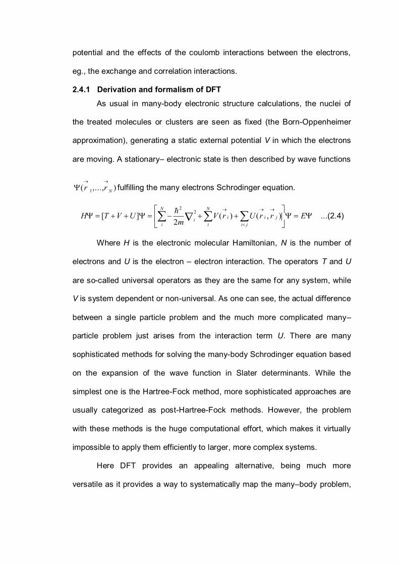
potential and the effects of the coulomb interactions between the electrons,
eg., the exchange and correlation interactions.
2.4.1 Derivation and formalism of DFT
As usual in many-body electronic structure calculations, the nuclei of
the treated molecules or clusters are seen as fixed (the Born-Oppenheimer
approximation), generating a static external potential V in which the electrons
are moving. A stationary– electronic state is then described by wave functions
),...,( 1 Nrr
fulfilling the many electrons Schrodinger equation.
ErrUrVm
UVTH ji
ji
i
N
ii
N
i
),()(2
][2
2 ...(2.4)
Where H is the electronic molecular Hamiltonian, N is the number of
electrons and U is the electron – electron interaction. The operators T and U
are so-called universal operators as they are the same for any system, while
V is system dependent or non-universal. As one can see, the actual difference
between a single particle problem and the much more complicated many–
particle problem just arises from the interaction term U. There are many
sophisticated methods for solving the many-body Schrodinger equation based
on the expansion of the wave function in Slater determinants. While the
simplest one is the Hartree-Fock method, more sophisticated approaches are
usually categorized as post-Hartree-Fock methods. However, the problem
with these methods is the huge computational effort, which makes it virtually
impossible to apply them efficiently to larger, more complex systems.
Here DFT provides an appealing alternative, being much more
versatile as it provides a way to systematically map the many–body problem,

with U, onto a single-body problem without U. In DFT the key variable is the
particle density )(
rn which is given by,
)...,,()...,,(...)( 22
*3
3
3
2
3
NNN rrrrrrrdrdrdNrn
...... (2.5)
Hohenberg and Kohn proved in 1964 [87] that the relation expressed
above can be reversed, i.e. to give ground state density )(0
rn it is in principle
to calculate the corresponding ground state wavefunction ),...( 10
Nrr . In other
words, 0 is a unique functional of 0n , i.e.
][ 000 n ...... (2.6)
and consequently all other ground state observable O are also functional of 0n
.][][][ 00000 nOnnO . ..... (2.7)
From this follows, in particular, that also the ground state energy is a
functional of 0n
][][][ 000000 nUVTnnEE ..... (2.8)
Where, the contribution of the external potential ][][ 0000 nVn can be
written explicitly in terms of the density.
.)()(][ 3rdrnrVnV ........ (2.9)
The functions T[n] and U [n] are called universal functions while V[n] is
obviously non-universal, as it depends on the system under study. Having
specified a system, i.e. V is known, one then has to minimize the functional,
.)()(][][][ 3rdrnrVnUnTnE ........ (2.10)

With respect to ),(
rn assuming one has got reliable expressions for T[n] and
U[n]. A successful minimization of the energy functional will yield the ground
state density ,0n and thus all other ground state observable.
The variational problem of minimizing the energy functional E[n] can be
solved by applying the Lagrangian method of undetermined multipliers, which
was done by Kohn and Sham in 1965 [88]. The functional in the equation
(2.10) can be written as a fictitious density functional of a non-interacting
system.
,][][][ nVTnnE sssss . ...... (2.11)
Where Ts denotes the non-interacting kinetic energy and Vs is an external
effective potential in which the particles are moving. Obviously, )()(
rnrns if
Vs chosen to be
Vs = V + U + (T-Ts)
Thus, one can solve the so-called Kohn-Sham equations of this auxiliary non-
interacting system
),()()(2
22
rrrV
miiis
. ..... (2.12)
which yields the orbitals i that reproduce the density )(
rn of the original
many-body system.
2
)()()(
rrnrn i
N
i
s
The effective single-particle potential sV can be written in more detail as
2
3( ')' [ ]
'
ss xc s
e n rV V d r V n r
r r
.... (2.13)

where the second term of equations (2.13) denotes, Hartree term describing
the electron Coulomb repulsion, while the last term xcV is called the exchange
correlation potential. Here, xcV includes all the many-particle interactions.
Since the Hartree term and xcV depend on )(rn , which depends on the i ,
which in turn depend on sV , the problem of solving the Kohn-Sham equation
has to be done in a self-consistent (i.e., iterative) way. Usually one starts with
an initial guess for )(
rn , then calculates the corresponding sV and solves the
Kohn-Sham equations for the i . From these values a new density can be
calculated and the whole process is started again. This procedure is then
repeated until convergence is reached.
2.4.2 Applications of DFT
Kohn-Sham theory can be applied in several distinct ways depending
on what is being investigated. In molecular calculations, a huge variety of
exchange–correlation functionals have been developed for chemical
applications. A popular functional widely used is B3LYP [81, 82, 89] which is a
hybrid method in which the DFT exchange functional, is combined with the
exchange functional from Hartree–Fock theory. These hybrids functional carry
adjusTable parameters, which are generally fitted to a training set of
molecules.
2.5 BASIS SET
In modern quantum chemical calculations are typically performed
within a finite set of basis functions. Gaussian 98 and other ab initio electronic
structure programmes use Gaussian type atomic functions as basis functions.
A basis set is the mathematical description of the orbitals within a system

(which in turn combine to approximate the total electronic wave functions)
used to perform theoretical calculation. The wave functions under
consideration are all represented as vectors, the components of which
correspond to coefficients in a linear combination of the basis functions in the
basis set used. The operators are then represented as matrices, in this finite
basis. When molecular calculations are preformed, it is common to use basis
composed of a finite number of atomic orbitals, centred at each atomic
nucleus within the molecule. Initially, atomic orbitals were typically slater
orbital, which corresponded to a set of functions, which decayed exponentially
with distance from the nuclei. These Slater-type orbitals could be
approximated as linear combinations of Gaussian orbitals. It is easier to
calculate overlap and other integrals with Gaussian basis functions and this
led to hug computational savings of the may basis sets composed of
Gaussian-type orbitals (GTOs), the smallest are called minimal basis sets and
they typically composed of the minium number of basis functions required to
represent all of the electrons on each atom.
The most common addition to minimal basis sets in the addition of
polarisaton functions, denoted by an asterisk, *. Two asterisks, **, indicate
that polarization functions are also added to light atoms (hydrogen and
helium). When polaristion is added to this basis set, a p-function is added to
the basis set. This adds some additional needed flexibility within the basis set,
effectively allowing molecular orbitals involving the hydrogen atoms to be
more asymmetric about the hydrogen. Similarly, d-type functions can be
added to a basis set with valance p-orbitals and f-functions to a basis set with

d-type orbitals and so on. The precise notation indicates exactly which and
how many functions are added to the basis set, such as (d.p)
Another common addition to basis sets is the addition of diffuse
functions, denoted by a plus sign, +. Two plus signs indicate that diffuse
functions are also added to light atoms (hydrogen and helium). These
additional basis functions can be important when considering anions and
other large, soft molecular system.
2.5.1 Minimal basis sets
A common naming convention for minimal basis set is STO-XG, where
X in an integer. This X value represents the number of Gaussian primitive
functions comprising a single basis functions. In these basis sets, the same
number of Gaussian primitives comprises core and valence orbitals. Minimal
basis sets typically give rough results that are insufficient for research quality
publication, but are much cheaper than their larger counter parts. The
commonly used minimal basis sets are:
STO – 2G
STO – 3G
STO – 6G
STO – 3G *-polarized version of STO-3G
2.5.2 Split valence Basis sets
During most molecular bonding it is the valance electrons, which
principally take part in the bonding. In recognition of this fact, it is common to
represent valance orbitals by more than one basis function. The notation for
these split-valance basis sets is typically X-YZg. In this case, X represents the
number of primitive Gaussians comprising each core atomic orbital basis

function. The Y and Z indicate that the valance orbitals are composed of two
basis functions each, the first one composed of linear combination of Y
primitive Gaussian functions, the other composed of a linear combination of Z
primitive Gaussian functions. In this case, the presence of two numbers after
the hyphens implies that this basis set is a split – valance double – zeta basis
sets are also used, denoted as X-YZWg, X-YZWVg etc., The commonly used
split-valance basis sets are:
3-21g
3-21g* - polarized
3-12+g – Diffuse functions
3-12+g *-with polarization and diffuse function
6-31g
6-31g*
6-31+g*
6-31g (3dt,3pd)
6-31G
6-31G*
6-311+g*
2.5.3 Double, Triple, Quadruple Zeta basis sets
Basis sets in which there are multiple basis functions corresponding to
each atomic orbital, including both valance orbitals and core orbitals or just
the valance orbitals, are called double, triple or quadruple-zeta basis sets.
Commonly used multiple Zeta basis sets are:
CC-PVDZ- Double – zeta
CC-PVDZ-triple-zeta

CC-PVQZ-quadruple-zeta
CC-PVSZ-quintuple-zeta
Aug-cc-pVDz- Augmented versions of the preceding basis sets with
added diffuse functions.
TZVPP-Triple-zeta
QZVPP-Quadruple –zeta
The ‘CC-P at the beginning of some of the above basis sets stands for
‘correlation consistent polarised’ basis sets. They are double/triple /
quadruple/quintuple-zeta for the valance obitals only and include successively
larger shells of polarization (correlating) functions (d, f, g etc.,) that can yield
convergence of the electronic energy to the complete basis set limit.
2.6 GAUSSVIEW
Gaussview is an affordable, full-featured graphical user interface for
Gaussian 03. With the help of Gaussview, one can prepare input for
submission to Gaussian and to examine graphically the output that Gaussian
produces.
The first step in producing a Gaussian input file is to build the desired
molecule. The bond lengths, bond angles, and dihedral angles for the
molecule will be used by Gaussview to write a molecular structure for the
calculation.
Gaussview incorporate an excellent Molecule Builder. Once can use it to
rapidly sketch in molecules and examine them in three dimensions. Molecules
can be built by atom, ring, group, amino acid and nucleoside.

Gaussview is not integrated with the computational module of
Gaussian, but rather is a front-end/back-end processor to aid in the use of
Gaussian. Gaussview can graphically display a variety of Gaussian
calculation results, including the following:
Molecular orbitals
Atomic charges
Surfaces from the electron density, electrostatic potential, NMR shielding
density, and other properties. Surfaces may be displayed in solid,
translucent and wire mesh modes.
Surfaces can be coloured by a separate property.
Animation of the normal modes corresponding to vibrational frequencies.
Animation of the steps in geometry optimizations, potential energy surface
scans, intrinsic reaction coordinate (IRC) paths, and molecular dynamics
trajectories from BOMD and ADMP calculations.
2.7 SCALING OF FORCE FIELDS
SQM, the method of scaled quantum mechanical force fields [76] is a
pragmatic approach to the ab initio based determination of molecular force
fields. Its basis idea is to use relatively low level ab initio calculations using
small basis sets and combine them with experimental information in the form
of an empirical adjustment, ‘scaling’ of the calculated force constants. SQM
force fields are of comparable accuracy with the best purely theoretical
results.
Quantum mechanical methods yield harmonic force constants. On the
other hand, the observed frequencies are anharmonic, but it is possible to
calculate the harmonic frequencies of small molecules from the observed
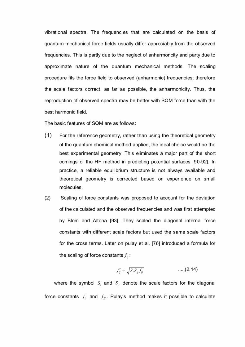
ij i j ijf S S f
vibrational spectra. The frequencies that are calculated on the basis of
quantum mechanical force fields usually differ appreciably from the observed
frequencies. This is partly due to the neglect of anharmoncity and party due to
approximate nature of the quantum mechanical methods. The scaling
procedure fits the force field to observed (anharmonic) frequencies; therefore
the scale factors correct, as far as possible, the anharmonicity. Thus, the
reproduction of observed spectra may be better with SQM force than with the
best harmonic field.
The basic features of SQM are as follows:
(1) For the reference geometry, rather than using the theoretical geometry
of the quantum chemical method applied, the ideal choice would be the
best experimental geometry. This eliminates a major part of the short
comings of the HF method in predicting potential surfaces [90-92]. In
practice, a reliable equilibrium structure is not always available and
theoretical geometry is corrected based on experience on small
molecules.
(2) Scaling of force constants was proposed to account for the deviation
of the calculated and the observed frequencies and was first attempted
by Blom and Altona [93]. They scaled the diagonal internal force
constants with different scale factors but used the same scale factors
for the cross terms. Later on pulay et al. [76] introduced a formula for
the scaling of force constants ijf :
.....(2.14)
where the symbol iS and jS denote the scale factors for the diagonal
force constants iif and jjf . Pulay’s method makes it possible to calculate

scale factors that are transferable between similar molecules if suiTable
internal coordinates are chosen.
(3) For systematic calculations, the same basis set should be used
consistently.
2.8 NORMAL COORDINATE ANALYSIS
Detailed description of vibrational modes can be studied by means of
normal coordinate analysis. Normal coordinate analysis is a procedure for
calculating the vibrational frequencies which relates the observed frequencies
of preferably the harmonic infrared and Raman frequencies to the force
constants, equilibrium geometry and the atomic masses of the oscillating
system. Normal coordinate analysis has proven useful in assigning vibrational
spectra but its predictive ability depends on having reliable intramolecular
force constants.
The problem of the normal vibrations of a polyatomic molecule is
satisfactorily dealt with, in particular, for small molecules by the method of
classical mechanics. The frequency of a molecular vibration is determined by
its kinetic and potential energies. The molecular vibrations are assumed to be
simple harmonic. Analysis of molecular vibrations from classical mechanics
will give valuable information for the study of molecular vibrations by quantum
mechanics because of the relationship between classical and quantum
mechanics.

2.8.1 Structure of molecule
Usually the structure of the molecule is available from x-ray studies or
electron diffraction studies. In case the structure is not available it is assumed
and the molecular parameters from the related systems are transferred.
2.8.2 Classification of normal modes
By applying Group theory, the point group symmetry of the molecule
and normal modes of vibrations are classified according to the irreducible
representations. Further these vibrations are distributed to various symmetry
species to which they belong. Applying IR and Raman selection rules, the
number of genuine vibrations under each species is determined.
2.8.3 Internal coordinates and symmetry coordinates
Internal coordinates are the changes in bond lengths and bond angles.
The symmetry coordinates are constructed from the internal coordinates and
they should be normalized and orthogonalised.
If R is a column matrix consisting of the internal coordinates and r is
the column matrix of the Cartesian coordinates, then
R Br
where B is the transformation matrix of the order (3n-6)* 3N, N being the
number of atoms in the molecule. If U is the orthogonal transformation matrix
and S is a column matrix of the symmetric coordinates, then S UR
2.8.4 Removal of Redundant Coordinates
The number of internal coordinates must be equal to or greater than
3N-6 (3N-5) degrees of vibrational freedom of molecule containing N atoms.
If more than 3N-6 (3N-5) coordinates are selected as the internal coordinates,
it implies that these coordinates are independent of each other. In complex

molecules it is very difficult to recognize a redundancy in advance. If a
sufficient number of internal coordinates is used, the number of redundancies
can be found by subtracting 3n-6 (the number of internal degrees of freedom)
from the number of internal coordinates. However, essential internal
coordinates may have been inadvertently omitted. If a molecule has any
symmetry, these considerations can be applied separately to each species.
The number of independent coordinates in each species can be obtained by
reducing the representation formed by the Cartesian coordinates and
subtracting the translations and rotations appropriately. The number of
internal symmetry coordinates is similarly obtained for each species, and any
excess represents redundancy. One very common form of redundancies is
also likely to appear in ring and these may involve the bond stretching
coordinates as well as the bond angles. In the software developed for solving
the vibrational secular equation, the redundant coordinates drop out as zero
roots of the secular equation when the symmetrized kinetic energy matrix is
diagonalized.
2.8.5 Potential energy matrix
The potential energy ‘V ’ of a molecule is the harmonic approximation
and is given by the expression,
2 ij i j
ij
V f r
where ijf are the force constants. This equation can be written in the matrix
form as,
FRRV 2
which becomes interms of symmetric coordinates as,
FSSV 2

where,
FUUF
UandSR , are the transposes of R ,S and U - matrices respectively
2.8.6 Kinetic energy matrix
The kinetic energy can be expressed in the form
SGST 12
where S is the derivative
t
Si of the jth internal coordinate 1G is the
inverse kinetic energy matrix obtained from B - matrix
BBMG 1
where 1M is a inverse diagonal matrix of masses of the atoms of the
molecule.
2.8.7 Secular equations
After evaluation the elements of potential and kinetic energy matrices,
the secular equation
0 EFG
is to be solved for evaluating the potential energy constants.
In the above equation E is the unit matrix and is a diagonal matrix
and it is related to the frequencies as
224 kk vC
2.8.8 Force constant refinement process
It is very difficult to solve the unsymmetrical FG- matrix in the secular
equation. Cyvin’s W - matrix method is followed to overcome this difficulty.
The G matrix is factorised into a non singular matrix such that
PPG

where
P is an upper triangular matrix
P is a lower triangular matrix
A trial F - matrix is set up by transferring the force constants from the
molecules of similar environment and by diagonalising the W - Matrix.
FPPW
and the values are obtained.
The process of successive approximation is continued till all the
calculated frequencies are in good agreement with the observed values. This
method introduces several non-vanishing off-diagonal elements in the F
matrix which are useful in calculating interaction force constants.
2.8.9 Computation of L Matrix
L-Matrix is obtained from the force field by factorising the
symmetrised G - matrix into a product of triangular matrices T and T
G PP F
G LL
but POL
where O is an orthogonal matrix
The secular equation 0FG E can be written in the form
LFL
POFPO
( )O PFP O
OWO

Here is a diagonal matrix containing eigen values of and FPP is
already defined. The O - matrix is obtained by diagonalising the W - matrix so
as to give the elements of matrix.
2.8.10 Potential energy distribution
In order to get the complete and accurate picture of the normal modes
of vibrations, the potential energy distribution (PED) has to be calculated in
the present investigation using the relation
a
iaiiLFPED
2
where
Fii is the potential energy constant
Lia is the L matrix element and
a is equal to 2224 avc
2.9 SCALING OF AB INITIO FORCE FIELDS BY MOLVIB
Quantum mechanical methods yield harmonic force constants. On
the other hand, the observed frequencies are anharmonic, but are possible to
calculate the harmonic frequencies of small molecules from the observed
vibrational spectra. The frequencies that are calculated on the basis of
quantum mechanical force fields usually differ appreciably from the observed
frequencies. This is partly due to the neglect of anharmonicity and the
approximative nature of the quantum mechanical methods.
Normal coordinate analysis is nowadays commonly employed as an
aid in the interpretation of the vibrational spectra of large molecules. In order
to get meaningful results, a knowledge of vibrational force field is necessary.
Since the number of force constants grows quadratically with the number of

atoms, one has to employ many approximations in the calculation of harmonic
force field even for moderately large molecules. To overcome this difficulty,
one can determine a force field for a set of related molecules using the
overlay method introduced by Snyder and Schachtschneider in the 1960’s
[94]. Gwinn developed a programme for normal coordinate analysis using
mass- weighted Cartesian coordinates [95], which eliminates the redundancy
problems arising when internal valance coordinates are used as in Wilson’s
GF-method. MOLVIB [96, 97], a FORTRAN programme is based on the
above idea developed for the calculation of harmonic force fields and
vibrational modes of molecules with upto 30 atoms. All the calculations are
performed in terms of mass weighted Cartesian coordinates, instead of
internal coordinates as in the conventional GF-method. This makes it possible
to overcome problems with redundant coordinates. The force field is refined
by a modified least squares fit of observed normal frequencies.
MOLVIB can be used for the scaling of vibrational force fields by
treating the scale factors as ordinary force constants. They can thus be
calculation from a least squares fit of the calculated and observed frequencies
[98]. To perform the scale factor calculations, the programme needs the
atomic coordinates, and the Cartesian force constants from an ab initio
calculation. An auxiliary programme (Rdarch) is used to extract these data
from the archive part of the out file of ab initio calculations. In addition, this
programme can also extract the dipole derivatives and the polarization
derivatives, which are needed for intensity calculations. MOLVIB will convert
the Gaussian force constants, which are expressed in atomic units into the
units used by the programme. Since the optimal values of the scale factors

usually are less than 1, it is good to start with an initial calculation, where all
the scale factors have been set to 1, and check that MOLVIB can reproduce
the frequencies calculated by the ab initio programme.
In MOLIVB, three methods are available for the scale factor
calculations. In two of these methods, the non diagonal terms in the potential
energy will depend non-linearly on the scale factors as,
1
2iji i i i j i j i j
i i j
V S f q q S S f q q¹
= +å å å … (2.13)
The factor i jS S that occurs in front of the non diagonal force constant has to
be repeated. The frequency fit usually converges in four or five iterations, and
often just a few repetitions are necessary. The initial values for the scale
factors are set to 1.
It is also possible to use individual scale factors for the non diagonal
force constants. In this case, scale factors should be associated both with
diagonal and non diagonal terms. Similar ideas have been proposed by Blom
and Altona [93]. However, too many different scale factors should not be used
in this case, but instead group similar factors together, so that the total
number of scale factors must be very minimum. The scale factors are
calculated from a least square fit of the observed vibrations in a similar way as
the force constants.