7

CHAPTER – II

Principles and classification of well logging methods

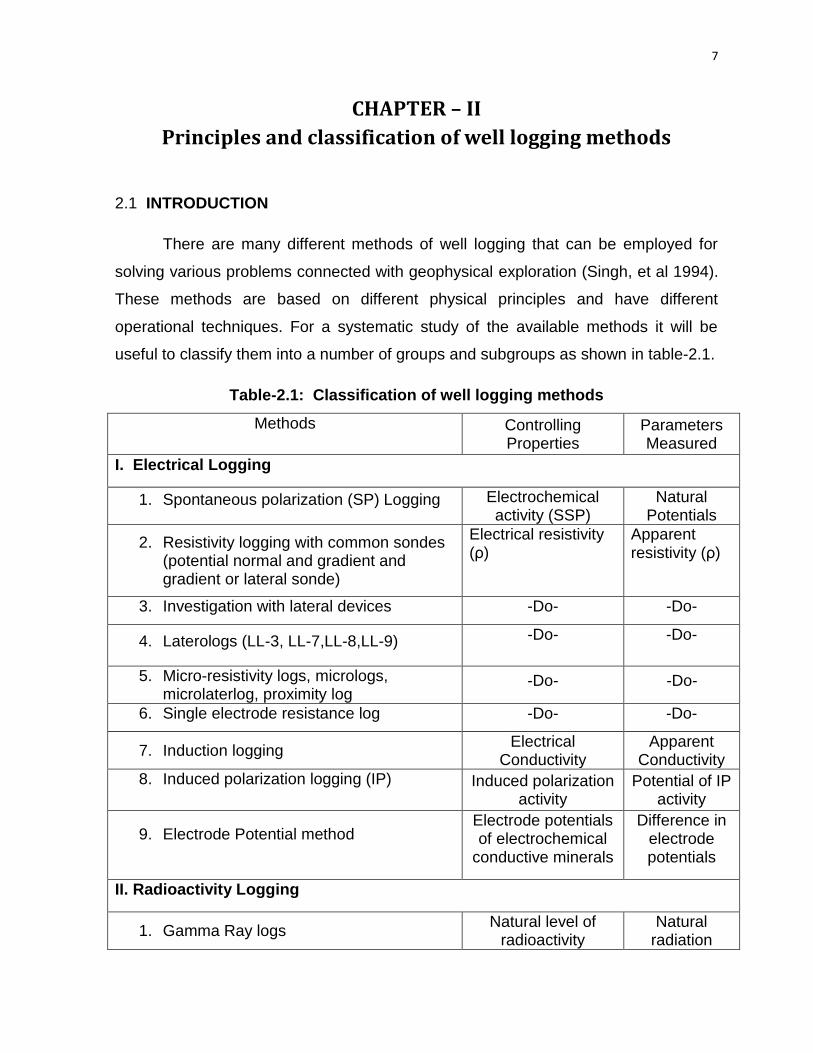
2.1 INTRODUCTION

There are many different methods of well logging that can be employed for

solving various problems connected with geophysical exploration (Singh, et al 1994).

These methods are based on different physical principles and have different

operational techniques. For a systematic study of the available methods it will be

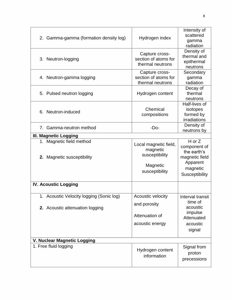
useful to classify them into a number of groups and subgroups as shown in table-2.1.

Table-2.1: Classification of well logging methods

Methods Controlling Properties

Parameters Measured

I. Electrical Logging

1. Spontaneous polarization (SP) Logging Electrochemical activity (SSP)

Natural Potentials

2. Resistivity logging with common sondes (potential normal and gradient and gradient or lateral sonde)

Electrical resistivity (ρ)

Apparent resistivity (ρ)

3. Investigation with lateral devices -Do- -Do-

4. Laterologs (LL-3, LL-7,LL-8,LL-9) -Do- -Do-

5. Micro-resistivity logs, micrologs, microlaterlog, proximity log

-Do- -Do-

6. Single electrode resistance log -Do- -Do-

7. Induction logging Electrical

Conductivity Apparent

Conductivity

8. Induced polarization logging (IP) Induced polarization activity

Potential of IP activity

9. Electrode Potential method Electrode potentials of electrochemical

conductive minerals

Difference in electrode potentials

II. Radioactivity Logging

1. Gamma Ray logs Natural level of

radioactivity Natural

radiation

8

2. Gamma-gamma (formation density log) Hydrogen index

Intensity of scattered gamma radiation

3. Neutron-logging Capture cross-

section of atoms for thermal neutrons

Density of thermal and epithermal neutrons

4. Neutron-gamma logging Capture cross-

section of atoms for thermal neutrons

Secondary gamma radiation

5. Pulsed neutron logging Hydrogen content Decay of thermal

neutrons

6. Neutron-induced Chemical

compositions

Half-lives of isotopes

formed by irradiations

7. Gamma-neutron method -Do- Density of

neutrons by

III. Magnetic Logging

1. Magnetic field method

2. Magnetic susceptibility

Local magnetic field, magnetic

susceptibility

Magnetic

susceptibility

H or Z component of

the earth’s magnetic field

Apparent

magnetic

Susceptibility

IV. Acoustic Logging

1. Acoustic Velocity logging (Sonic log)

2. Acoustic attenuation logging

Acoustic velocity

and porosity

Attenuation of

acoustic energy

Interval transit time of

acoustic impulse

Attenuated

acoustic

signal

V. Nuclear Magnetic Logging

1. Free fluid logging

Hydrogen content

information

Signal from

proton

precessions

9

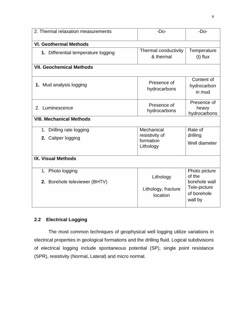
2. Thermal relaxation measurements -Do- -Do-

VI. Geothermal Methods

1. Differential temperature logging Thermal conductivity

& thermal

Temperature

(t) flux

VII. Geochemical Methods

1. Mud analysis logging Presence of

hydrocarbons

Content of

hydrocarbon

in mud

2. Luminescence Presence of

hydrocarbons

Presence of heavy

hydrocarbons

VIII. Mechanical Methods

1. Drilling rate logging

2. Caliper logging

Mechanical resistivity of formation Lithology

Rate of drilling

Well diameter

IX. Visual Methods

1. Photo logging

2. Borehole televiewer (BHTV) Lithology

Lithology, fracture

location

Photo picture of the borehole wall Tele-picture

of borehole

wall by

2.2 Electrical Logging

The most common techniques of geophysical well logging utilize variations in

electrical properties in geological formations and the drilling fluid. Logical subdivisions

of electrical logging include spontaneous potential (SP), single point resistance

(SPR), resistivity (Normal, Lateral) and micro normal.

10

2.3 Spontaneous potential logging

The spontaneous potential log (SP) is a record of potentials or voltages that

develop at the contacts between shale or clay beds and a sand aquifer, where they

are penetrated by a borehole.The natural flow of current and the spontaneous

potential curve that would be produced under the salinity conditions. The SP

measuring equipment consists of a lead electrode in the well connected through a

milli voltmeter to a second lead electrode that is grounded at the land surface.

The spontaneous potential is a function of the chemical activates of fluids in the

borehole and adjacent rocks, the temperature, and the type and quantity of clay

present. The chief source of SP in a borehole is electrochemical and electro kinetic or

streaming potentials. (Doll, 1948; Daknov, 1959) Electrochemical effects probably are

the most significant contributor; they can subdivide into membrane and liquid junction

potentials. Both these effects are the result of the migration of ions from concentrated

to more dilute solution, and they are mostly affected by clay, that decreases negative

(anion) mobility. Membrane potentials are developed from formation water to

adjacent shale, for fluid in the borehole; a three component system. Liquid junction

potentials are those developed between the filtrate in the invaded zone and the

formation water. If the fluid column in the borehole is more saline than the water in

the aquifer, current flow and the log will be reversed. Streaming potentials are caused

by the movement of an electrolyte through permeable media. They are substantial at

depth intervals where water is moving in or out of the hole.

The SP logs have been used widely in determining lithology, bed thickness

and the salinity of the formation water (Roy et al, 1975; Silva et al, 1981). Lithologic

contacts are located on spontaneous potential logs at the point of curve inflection,

where the current density is maximum. When the response is typical, a line can be

drawn through the positive spontaneous potential values recorded in shale base line

and a parallel line may be drawn through negative values that represent intervals of

the sand base line containing little clay. If salinity and the composition of the borehole

and the interstitial fluids are constant through the logged interval, shale and sand

lines will vertically on the log; however, this is not common in water wells (Guyod,

11

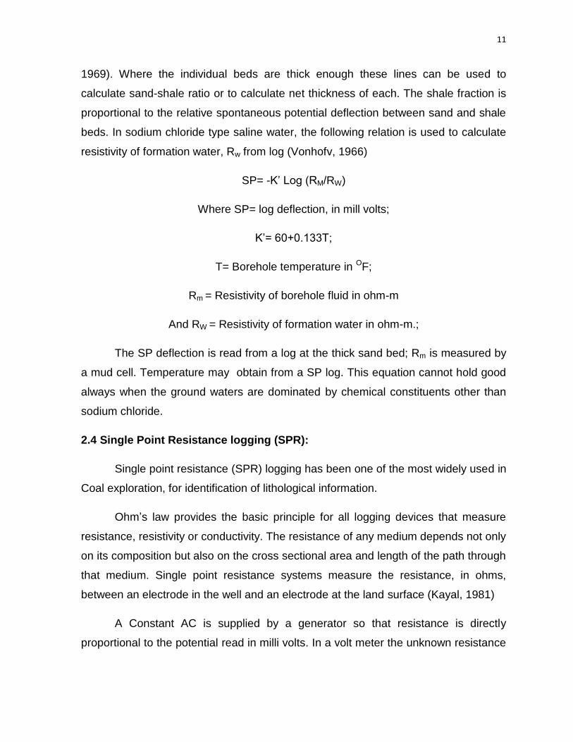
1969). Where the individual beds are thick enough these lines can be used to

calculate sand-shale ratio or to calculate net thickness of each. The shale fraction is

proportional to the relative spontaneous potential deflection between sand and shale

beds. In sodium chloride type saline water, the following relation is used to calculate

resistivity of formation water, Rw from log (Vonhofv, 1966)

SP= -K’ Log (RM/RW)

Where SP= log deflection, in mill volts;

K’= 60+0.133T;

T= Borehole temperature in OF;

Rm = Resistivity of borehole fluid in ohm-m

And RW = Resistivity of formation water in ohm-m.;

The SP deflection is read from a log at the thick sand bed; Rm is measured by

a mud cell. Temperature may obtain from a SP log. This equation cannot hold good

always when the ground waters are dominated by chemical constituents other than

sodium chloride.

2.4 Single Point Resistance logging (SPR):

Single point resistance (SPR) logging has been one of the most widely used in

Coal exploration, for identification of lithological information.

Ohm’s law provides the basic principle for all logging devices that measure

resistance, resistivity or conductivity. The resistance of any medium depends not only

on its composition but also on the cross sectional area and length of the path through

that medium. Single point resistance systems measure the resistance, in ohms,

between an electrode in the well and an electrode at the land surface (Kayal, 1981)

A Constant AC is supplied by a generator so that resistance is directly

proportional to the potential read in milli volts. In a volt meter the unknown resistance

12

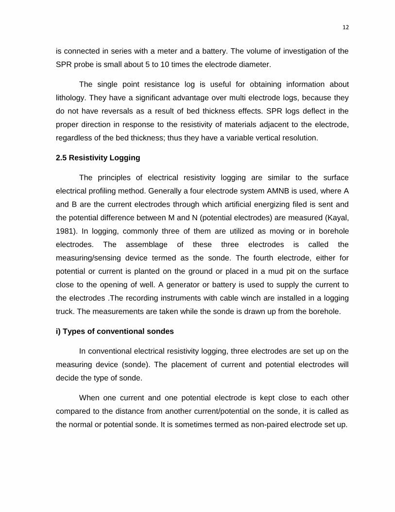
is connected in series with a meter and a battery. The volume of investigation of the

SPR probe is small about 5 to 10 times the electrode diameter.

The single point resistance log is useful for obtaining information about

lithology. They have a significant advantage over multi electrode logs, because they

do not have reversals as a result of bed thickness effects. SPR logs deflect in the

proper direction in response to the resistivity of materials adjacent to the electrode,

regardless of the bed thickness; thus they have a variable vertical resolution.

2.5 Resistivity Logging

The principles of electrical resistivity logging are similar to the surface

electrical profiling method. Generally a four electrode system AMNB is used, where A

and B are the current electrodes through which artificial energizing filed is sent and

the potential difference between M and N (potential electrodes) are measured (Kayal,

1981). In logging, commonly three of them are utilized as moving or in borehole

electrodes. The assemblage of these three electrodes is called the

measuring/sensing device termed as the sonde. The fourth electrode, either for

potential or current is planted on the ground or placed in a mud pit on the surface

close to the opening of well. A generator or battery is used to supply the current to

the electrodes .The recording instruments with cable winch are installed in a logging

truck. The measurements are taken while the sonde is drawn up from the borehole.

i) Types of conventional sondes

In conventional electrical resistivity logging, three electrodes are set up on the

measuring device (sonde). The placement of current and potential electrodes will

decide the type of sonde.

When one current and one potential electrode is kept close to each other

compared to the distance from another current/potential on the sonde, it is called as

the normal or potential sonde. It is sometimes termed as non-paired electrode set up.

13

If a pair of current or potential electrodes are kept close together compared to

the third potential/current electrode. It is called a lateral or gradient sonde. Some-

times it is termed as paired electrode set up.

Normally the third electrode is kept at least five times the distance away from

the other two closely spaced electrodes. Depending on the number of current

electrodes on the sonde, it is also known as a unipolar or bipolar sonde.

For normal/potential sonde, the distance AM is called the length of the sonde

and for lateral/gradient sonde; the distance AO is the length of the sonde, where ‘0’ is

the mid point of the paired electrodes.

Conventional lengths of the sounde are AM=16’’ and 64’’ and AO = 18.8’’.

AM=16’; is called as the short normal and AM = 64’’ is called as the long normal. The

lengths of the sondes can be altered.

ii) Curve characteristics

The shape of resistivity curve depends on the type of sonde

(potential/gradient), and the ratio of the following:

i. The formation resistivity to the resistivity of the surrounding formation

(Rt/Rs)

ii. The resistivity of the formation to the borehole mud resistivity (Rt/Rm).

iii. The length of the sonde to the borehole diameter (L/d)

iv. The thickness of the formation to diameter of the borehole (h/d).

Thick beds are those whose thickness is larger compared to the length of

the sonde and thin beds are the ones wherein the length of the sonde is

larger compared to its thickness.

Apparent resistivity curves for resistive and conductive formations and for

thick and thin beds are different for potential and gradient sondes.

14

a) Normal potential sonde

The shape and amplitude of the curves depend on the resistivity contrast and

the thickness of the target formation. In case of resistive formation of finite thickness

(i.e., length of the sonde very small) the bed boundaries are determined by adding

half the sonde length on either side of the borehole inflection point and the resistive

bed appears one spacing length thinner than the actual thickness of the bed. The

shape of the curve is symmetrical to the center of the bed boundaries.

If the formation is thin compared to the spacing of the sonde used and

resistive, the curve appears as if the bed is conductive and much thicker. On either

side of the bed, we have symmetrical resistive peaks. The boundaries are located by

reducing half the electrode length from these peaks. In practice the peaks are poorly

recorded and hence demarcation of thin formations becomes difficult.

If the target formation is by conductive nature and of finite thickness, the actual

bed boundaries are located by subtracting half the spacing of the sonde on either

side of the inflection point. Thus, conductive beds always appear thicker by one

electrode spacing than their actual thickness.

b) Lateral / Gradient Sonde

The curve shapes for the gradient sonde are asymmetrical and their shapes

depend on the position of the in the borehole current electrode. Two types of gradient

sonde are possible, the top sensing gradient sonde and the bottom sensing gradient

sonde. When the bed thickness is large compared to the length of the sonde and the

formation is resistive, the gradient curves have the following characteristics in case of

a bottom sensing gradient sonde.

At the upper boundary, the resistivity recorded has a minimum and the value

of this minimum is less than the resistivity of the adjacent bed.

Opposite the bed, the apparent resistivity values increases from top to the

bottom of the bed. This increase is small in the beginning (up to the length of the

15

sonde (AO) from the top of the bed) and then as the inhole electrode passes through

the center of the bed, the increase resistivity value is very sharp.

At the lower boundary, the resistivity curve has a maximum and below the

boundary the resistivity value falls down sharply and attains a value representing the

resistivity of the abject formation.

The curve characteristics will be vice-versa in the case of a top gradient

sonde.

c) Characteristic value of apparent resistivity for beds of finite thickness

Apparent resistivity recorded opposite a bed varies from point to point. In

practice, we use the following characteristic values of apparent resistivity.

The maximum and minimum apparent resistivity values are used for resistive

and conductive beds. For a resistive bed on the potential sonde curve, maximum

value is recorded against the mid-point of the bed. On the gradient log, the maximum

value will be at the lower boundary in case of bottom sensing gradient sonde and at

the upper boundary in case of top sensing gradient sonde.

In case of a potential sonde curve for conductive bed, the minimum value is

recorded at the mid-point of the bed and for gradient sonde the minimum value is at

the boundary.

The average resistivity of a bed is generally obtained by finding the area

bounded by the curve and the depth axis and then dividing it by the thickness of the

formation.

In practice, by first locating the upper and lower boundaries and then a straight

line parallel to the depth axis is so drawn that it cuts the line representing the top and

bottom boundary of the bed such that the area of triangle between the top of the bed

and the curve is equal to the area bounded by the curve diagonally opposite it. In

such a case the area of the rectangle so formed is equal to the area bounded by the

16

curve. The resistivity value at the point of intersection of this line with the apparent

resistivity curve represents the average resistivity value for the bed.

Optimum resistivity is the value that is close to the true resistivity of the layer. It

corresponds to the value at a point on the curve approximately half the spacing of the

sonde above the mid-point of the bed (top sensing gradient sonde) or half the

spacing of the sonde below the midpoint of the formation (bottom sensing gradient

sonde). The average resistivity value and the optimum resistivity value are usually

determined for beds whose thickness is more than the length of gradient sonde

(Kayal, J.R. and Christoffel, D.A.1989)

d) Determination of true resistivity of formation

Four main factors are needed to deduce the true resistivity ‘R’ they are

average of apparent resistivity Ra mud resistivity (Rm), the diameter of the borehole

(d) and the spacing AM or AO with which Ra is measured. The value of Ra over

formation is to be determined from the electric log, taking the average value where

small variation is present. If the bed thickness is at least four times the spacing of the

normal device or at least two times the spacing of the lateral device, Ra is used to

determine the true resistivity. The value of Rm is corrected for the temperature at the

depth of the formation. The borehole diameter d can be determined using caliper log

drill bit diameter can be taken. The electrode spacing, AM or AO is normally shown

on the log heading.

In practice, normally two types of situation occur:

i) Without invasion

ii) With invasion in the formation of interest

Master curves known as departure curves are used for the determination of the

resistivity Rt for different levels of invaded zone.

In the present work, the charts given in the manual “Formation evaluation data

hand book” published by Guyod (1952) are used in correcting the formation

resistivities for the borehole diameters.

17

2.6 Radio Active Logging

Geophysical methods of investigation of well section using the natural or

artificially produced nuclear radiation are known as radioactive, radiation logging or

nuclear logging. Gamma rays and neutrons are the two important nuclear radiations

measured in well logging. These two radiations have a unique ability to penetrate

high density material such as rocks, well casing and cement. Radioactive logs can be

used either in cased wells or open wells. Since no direct contact with the formation is

necessary, any type of bore well containing air, water or drilling mud can be logged.

Electrical logging in contrast, can be done only in uncased boreholes filled with

drilling mud.

Radioactive logs can be obtained from old wells where original logs were not

taken.While a wide variety of nuclear logging techniques are employed in oil industry

only a few of them are useful in logging water wells. They are:

1. Gamma ray logging

2. Gamma-Gamma logging

3. Neutron logging

a) Neutron- neutron logging

b) Neutron gamma logging

2.6.1 Gamma Ray Logging

Natural gamma logs are the most widely used nuclear logs in ground-water

application. The most common uses are for identification of lithoglogy and for

stratigraphic correlation. Gamma logs can be made with relatively inexpensive and

simple equipment, and they will provide useful data under a variety of borehole

conditions.

The gamma log provides a record of the total gamma radiation detected in a

borehole. In water-bearing formation that are not contaminated by artificial

18

radioisotopes, the most significant naturally occurring, gamma-emitting radioisotopes

are Potassium-40 and daughter products of the uranium and thorium decay series.

Fine grained detrital sediments that contain abundant clay tend to be more

radioactive than quartz, sand carbonate rocks, although numerous exceptions occur.

Rocks can be characterized according to their usual gamma intensity. Limestone,

and dolomite usually are less radioactive than shale; however, all these rocks can

contain deposits of uranium and be quite radioactive. Basic igneous rocks usually are

less radioactive a silica igneous rocks, but expectations are known. Several reasons

exist for a considerable variation in the radioactivity of rocks.

The volume of material investigated by a gamma probe is related to the

energy of the radiation measured, the density of the material through which that

radiation must pass, and the design of the probe. Dense rock, steel casing and

cement will decrease the radiation that reaches the detector, particularly from a

greater distance from the borehole. Under most conditions, 90 percent of the gamma

radiation detected probably originates from material within 6 to 12 inches of the

borehole wall. The volume of material contributing to the measured signal may be

considered approximately spherical, with no distinct boundary on the outer surface.

The vertical dimension of this volume also will depend on the length of the crystal,

which will affect the resolution of the thin beds. Because the detector is the center of

the volume investigated, radioactivity measured when the detector is located at a bed

contact will be an average of the two beds. The actual radioactivity of beds with a

thickness less than twice the radius of investigation will not be recorded.

The API gamma-ray unit is defined as 1/200 of the difference in deflection of a

gamma log between an interval of negligible radioactive proportions of radioisotopes

as an average shale but about twice the total radioactivity. One or more filed

standards is needed when calibrating in a pit or well (Belknap et al, 1959; Crew et al,

1970) and when calibration frequently during logging operations to assure that a

gamma logging system is stable with respect to time and temperature. Field

standards may consist of radioactive sources that can be held in one or more fixed

position in relation to the detector while readings are made. If this approach is used,

19

the probe is best located at least several feet above the ground and distant from a

logging truck that contains other radioactive sources that could contribute to the

background radiation. Radiation measurements around the logging truck will

determine the proper distance.

Because of numerous deviations from the typical response of gamma logs

to lithology, some background information on each new study area is needed to

decrease the possibility of errors in interpretation (Wahl, 1983)

In igneous rocks, gamma intensity is greater in silica rocks, such as granite,

than in basic rocks. Orthoclase and biotite are two minerals that contain

radioisotopes of sedimentary rocks of chemical decomposition has not been too great

Gamma logs are used widely in the petroleum industry to establish the clay or

shale content of reservoir rocks; (Moore, 1980; and Killen, 1982) this application also

is valid in coal exploration studies.

The increase in radioactivity from an increase in fine grained materials has

been the basis for a number of studies relating gamma log response to permeability

in various parts of the world, such as the Denver Julesberg basin in Colorado, Texas,

USA, India and Russia (Rabe, 1957; Raplova 1961; Gour et al, 1965; and Keys et al,

1973:)

2.7 Gamma – Gamma logging

Gamma-Gamma logs (also known as density logs) are records of the intensity

of gamma radiation from a source in the probe after it is back scattered and

attenuated within the borehole and surrounding formation. The main uses of gamma-

gamma logs are for identification of lithology and the measurement of the bulk

density and porosity of rocks. These logs may also be used for locating cavities and

cement outside the casing of well.

The gamma-gamma probe contains a source gamma rays, generally Cobalt-

60 or Cesium-137, shielded from sodium iodide detector by Mallory-1000 metal or

lead spacers. Gamma rays from the source penetrate and are scattered and

20

absorbed by the fluid, casing and formatting surrounding the probe. Gamma radiation

is absorbed and (or) scattered by all material through which travels. Degradation of

photon energy takes place by three main processes.

1. The Compton scattering, in which a gamma rays less part of its energy to an

orbital electron (z) and occurs with gamma photons from 01. To 1 mev.

2. The photoelectric effect, in which an ejected orbital electron completely

absorbs the photon energy, is proportional to Z4.5 and occurs with photons 0.1

mev or less.

3. Pair production, which occurs as the photon approaches the nucleus and

completely converts itself into a pair of electrons, is proportional to Z2 and

requires gamma energy greater than 1.02 mev.

Compton scattering is probably the most significant process taking place in

gamma-gamma logging. Some photoelectric absorption also takes place

because of degradation of photon energy by scattering, but the effect on a log

may be reduced by energy discrimination. In the Compton range the gamma

radiation absorbed is proportional to the electron density of the material

penetrated, but it is affected by the chemical nature of the medium. The

electron density is approximately proportional to the bulk density of most

materials penetrated in logging.

The Gamma-gamma log can also be used to identify borehole enlargements

through casing. The water level and significant change in fluid density will also

apparent on gamma-gamma logs.

In gamma-gamma logging the relative percentage of gamma photons

absorbed and scattered depends to a large degree upon the type and size of the

source, spacing between the source and detector, and the borehole diameter. The

radius of investigation depends on these same factors in addition to the bulk density.

In general source strength large diameter holes.

21

Modern gamma-gamma probes are decentralized and side collimated. Side

collimation with heavy metal tends to focus the radiation from the source and to limit

the detected radiation to that part of the wall of the borehole in contact with the

source and detectors. The decentralizing caliper arm also provides a log of hole

diameter. The decentralized tool has the advantage of being much less affected by

changes in drill-bit size, sonde position in the hole, or density of fluid in the hole.

The gamma-gamma loggers can be calibrated in terms of density by

comparing the probe responses against known formation with densities of core

samples from the same spot (Head et al, 1980). Measurements of two to three

different formations, with their densities covering the density range of interest, are

required for constructing the calibration graph in semi-log scale.

The gamma gamma logs can be used to determine the formation porosity

using the relation:

Porosity = grain density – Bulk Density (from log) /Grain density-fluid density

Grain density can be derived from laboratory analysis of cores or cuttings. The

fluid density in most water wells may be assumed to be l gm/cc. If the fluid is highly

saline, laboratory measurement of density may be necessary. If the same lithologic

unit is present below and above the water table, or if gamma-gamma measurement

can be made after the drawdown, it should be possible to derive specific yield from

gamma-gamma log (Davis, 1967) specific yield should be proportional to the

difference between the bulk density of saturated and drained sediments, if the

porosity, and grain density are not changed. Bulk density may be read directly from a

calibrated and corrected log or derived from a chart providing correction factors.

Errors in bulk density obtained by gamma-gamma methods are of the order of +/-

0.03-0.04 gm/cc. Errors in porosity calculated from log bulk densities depend on the

accuracy of grain and fluid densities used. For certain source to detector spacing’s

and over a limited density range, a linear relationship is obtained when bulk density is

plotted against the logarithm of count rate. In addition to determining porosity, the

22

gamma-gamma log may be used to locate casing or collars or the position or the

position of grout outside of the casing.

2.8 Neutron Logging

In neutron logging a neutron source is lowered along with the detectors into

the borehole. The source is fixed at the end of the probe and above it the counters

are placed. The spacing between the neutron source and counters may be 12 to 27’’.

Depending upon the recording capability of the counters used in the neutron probe,

three different types of neutron logs are possible. These are the neutron gamma log,

the neutron thermal neutron log and the neutron epithermal neutron log. The neutron

logs are chiefly used for the measurement of moisture content above the water table

and porosity below the water table. In most of the modern logging equipments

Americium-Beryllium source 1066 neutrons per second and the half life of the source

is 458 years. So the decay correction factor is very small the source emits fast

neutron emits fast neutrons having an average energy level of the order of 105ev.

Various types of neutron logs are made by counting neutrons present at

different energy levels (Kayal, 2002) the neutron thermal neutron probe responds

chiefly to thermal neutrons i.e., the neutron having energy level between 0.025 Mev

and 0.1Mev and the neutron epithermal neutron tool responds mostly to the neutrons

having energy level between 0.1 ev and 100ev. The neutron-neutron logs do not

have the problem of shielding the counters from the gamma radiation of the source

since the counters used in this type of logging system are not sensitive to gamma

radiation. In the neutron thermal neutron log, the neutrons are determined with a

proportional counter after they reach thermal energy level. While in the case of

neutron epithermal neutron log the counter measures the neutrons just before they

reach the thermal level. The counters used in this type of instruments are scintillation

counters. The neutron thermal neutron log is sensitive to the variation in the capture

cross section of the formation elements while the neutron epithermal neutron log is

completely insensitive to variation in capture cross section because it measures the

neutron at an energy level before the reaction take place (Krishnan, 1982).

23

2.8.1) Radius of investigation

The radius of investigation of neutron device is from 6 inches for high porosity

saturated formation to 2 feet for low porosity or dry rocks. The neutron logs are the

most useful techniques as applied to ground water investigations, because most of

the probe response is due to hydrogen and therefore water

Use:

1. The neutron logs are chiefly used for the measurement of moisture content

above the water table and total porosity below the water table.

2. The combined study of thermal neutron log and natural gamma ray log

helps in differentiating the formations from each other. The gypsum and

anhydrite both emit very low intensity gamma radiation and on the logs

they will have the same counting level which makes it difficult to interpret

the logs. But if the thermal neutron log of the same borehole is available it

is possible to differentiate them because the anhydrite gives low counting

rate while the gypsum gives high counting rate. Thus comparison of these

logs helps in making quantitative interpretation of the log.

3. The epithermal neutron logs provide the highest percentage of response

due to hydrogen and are least affected by the chemical composition of

rocks and the fluids they contain.

4. The neutron gamma ray log is very sensitive to chloride content, while the

neutron epithermal neutron log is insensitive to the chemical composition of

fluids. This comparison of these two logs reveals the presence of chloride

in the formation. In petroleum logging the direct comparison of neutron-

neutron logs with neutron gamma logs gives the idea about saline

formation water because the increase in count rate on the neutron gamma

ray log is supposed to be due to chlorine and thus due to NaCl

concentration. (Meyers, 1982) described how neutron logging devices can

be used to determine the specific yield of unconfined aquifers.

24

5. A conventional pumping test neutron logging methods were used

simultaneously to determine the specific yield of the aquifer in the alluvium

formation. Before the pumping test was stated the moisture percentage by

volume was determined with neutron log for each foot of depth of the

saturated zone. The pumping test was then carried out and the amount of

water pumped out was then measured. Then again the neutron log was run

and the moisture percentage was determined. The specific yields

calculated by pumping test data and by neutron logging were very close to

each other.

2.9 Caliper Logging

Caliper logs provide a continuous record of borehole diameter and are used

extensively for ground water application. Changes in borehole diameters may be

related to both drilling technique and lithology. Caliper logs are essential to guide the

interpretation of other logs, because most of them are affected by changes in

borehole diameter. Caliper logs also are useful in providing information on well

contraction, lithology, and secondary porosity. Many different types of caliper logs

are described in detail by (Hilchie, 1968). Single arm caliper probes commonly are

used to provide a record of borehole diameter, while running another type of log.

The single arm also may be used to decentralize a probe, such as a side collimated,

gamma-gamma probe. This probe has advantages in this the arm generally follows

the high side of a deviated hole. A three arm averaging caliper probe does not

function properly in highly deviated boreholes, because the weight of the tool forces

on arm to close, which closes the other two arms.

Calibration of caliper probes is done most accurately in rings of different

diameters. Because large cylinders occupy considerable space in a logging truck, it

is common practice to use a metal plate for on-site calibration. The plate is drilled

and marked every inch or two and machined to fit over the body of the probe, one

arm is placed in the appropriate holes in the range to be logged; the pen location is

labeled on the analog chart and a digital value is recorded, if applicable.

25

Heavy drilling mud will prevent caliper arms from opening fully and thick mud

cake may prevent accurate measurement of drilling diameter.

A Caliper log is needed to interpret many other logs, it needs to be made

before the casing is installed in borehole that is in danger of caving. When borehole

conditions are questionable, the first log made generally is the single point resistance

logs, because it will provide some lithology information; the probe is relatively in-

expensive, if it is lost. If no serious caving problems are detected during the running

of the single point resistance log, a caliper log needs to be run before the casing is

installed so it can be used to aid the analysis nuclear logs made through the casing.

Data for extremely rough intervals of the borehole wall, with changes in diameter of

several inches, cannot be corrected based on caliper logs; data for these intervals

need to be eliminated from quantitative analysis.

Caliper logs can provide information on lithology and secondary porosity. Hard

rocks like limestone will have a smaller diameter than adjacent shales. Thin beds

may result in an irregular trace. Secondary porosity, such as fractures and solution

openings, may be obvious on a caliper log. Caliper logs have been used to correlate

major producing aquifers in the Snake River plain in Idaho (Jones, 1961). Vesicular

and Scoriaceious tops of basalt flows, cinder beds, and caving sediments were

identified with three arm caliper logs. In the basalt of the quaternary snake river

group, caliper logs also were used to locate the optimum depth for cementing and to

estimate the volume of cement that might be required to fill the annals to a

preselected depth (Keys, 1963).

Similarly a caliper log is used to calculate the volume of gravel pack needed

and to determine the size of casing that can be set to select the depth.

2.10 Temperature Logging

Temperature logs can provide useful information on the movement of water

through a borehole, including the location of depth intervals that produce or accept

water (Watney, 1979). Thus, they can provide information related to permeability

distribution and relative hydraulic head. Temperature logs can be used to trace the

26

movement of injected water or waste, to locate the cement behind casing and to

correct other logs that are sensitive to temperature. Though the temperature sensor

only responds to the temperature of the water or air in the immediate vicinity,

recorded temperatures may indicate the temperature of adjacent formation and their

contained fluids. Formation temperature may be indicated if no flow exists in the

borehole and if equilibrium exists between the temperature of the fluid and the

temperature of the adjacent rocks.

The differential temperature log can be considered the first derivative of the

temperature log; it can be obtained by two different types of logging probes or by

computer calculation from a temperature log. Logging speed needs to be maintained

accurately for this method departure from the reference gradient will be recorded as

deflections on the log.

Temperature logs can aid in the solution of a number of ground water

problems if they are properly run under suitable conditions and if interpretation is not

over simplified. If there is no flow in or adjacent to borehole, the temperature

gradually will increase with depth, as a function of the geothermal gradient. Typical

geothermal gradients range between 0.47 to 0.60C/100 ft of depth; they are related to

the thermal conductivity or thermal resistivity of the rocks adjacent to the borehole

and the geothermal heat flow from below. Conway (1977) developed a computer

program for correcting digitized temperature data, calculating temperature gradient or

differential temperature logs.

Temperature data from wells are also used to calculate water density,

viscosity, and thermal conductivity and to develop heart flow maps, which can be

used to estimate the fluid flux, particularly, in geopressured aquifers.