5

CHAPTER II

LITERATURE REVIEW

2.1 Remote Sensing

The concept of remote sensing method is to obtain information about

properties of an object without coming into physical contact with the object.

Remote sensor devices are used in order to study large areas of the Earth’s

surface. These sensors are mounted on platforms such as helicopters, planes, and

satellites that make it possible for the sensors to observe the Earth from above.

The technique of remote sensing are developed to receive and analyze the

information which had the shape of electromagnetic wave radiation that was

broadcasted or reflected from the surface of the Earth.

2.1.1 Definition and Methods of Remote Sensing

The term of remote sensing is commonly used to describe the science and

art of identifying, observing, and measuring an object without coming into direct

contact with it. This process involves the detection and measurement of radiation

of different wavelengths reflected or emitted from distant objects or materials, by

which they may be identified and categorized by class or type, substance, and

spatial distribution (Graham, 1999). A more specific definition of remote sensing

relates to studying the environment from a distance using techniques such as

satellite imaging, aerial photography, and radar (Hoang and Ashley, 2012).

6

The process of data collection by using remote sensing can be seen in

Figure 2.1 below.

Figure 2.1 Data Collection by Using Remote Sensing

(Source: Lilesand and Kiefer, 1993)

The detector of remote sensing is called sensor. Information about an

object, an area, and a phenomenon are observed from the analysis of the data

which are gathered by the sensor from the long distance. The sensor is installed to

the vehicle (platform) that could have the shape of an aircraft, a rocket, an air

balloon or a satellite. It will receive and record the reflection and electromagnetic

radiation emission that came from the object. Further the data are analyzed in

order to get the specific information. The integrity sizes of electromagnetic

radiations that are reflected (reflection), passed (transmission) and broadcasted

(emission) were different for each object. It depends on the characteristics of the

object and the wavelength to the object (Campbell and Wynne, 2011). There are a

number of important stages in a remote sensing process (Aggarwal, 2005):

7

a. Emission of electromagnetic radiation (EMR) that is sun or self-emission.

b. Transmission of energy from the source to the surface of the earth, as well as

absorption and scattering.

c. Interaction of EMR with the earth’s surface such as reflection and emission.

d. Transmission of energy from the surface to the remote sensor.

e. Sensor data output.

2.1.2 Platform

Platforms refer to the structures or vehicles on which remote sensing

instruments are mounted. The platform determines a number of attributes, which

may dictate the use of particular sensors. These attributes include distance of

sensor from the object of interest, periodicity of image acquisition, timing of

image acquisition, and location and extent of coverage. There are three broad

categories of the platforms namely ground based, airborne, and satellite. A wide

variety of ground based platforms are used in remote sensing, such as hand held

devices, tripods, towers and cranes. Airborne platforms such as airplanes were the

sole non-ground-based platforms for early remote sensing work. The most stable

platform aloft is a satellite, which is spaceborne (CCPO, 2003).

Over a hundred remote sensing satellites have been launched. Terra, Aqua,

SPOT (Satellite Pour l'Observation de la Terre), IKONOS, and ALOS (Advanced

Land Observation Satellite) are some of the satellite platforms that mainly used in

remote sensing. ALOS is referred to a circular orbit satellite and its flight altitude

is over 500-1,000km (Iseki, 2013).

8

2.1.3 Passive and Active Sensors System

Sensors are remote sensing instrument which are mounted on platforms to

be able to observe the Earth from above. The remote sensors gather information

by measuring the electromagnetic radiation that is reflected, emitted and absorbed

by objects in various spectral regions, from gamma-rays to radio waves. There are

two types of sensors which are used to measure this radiation, namely active and

passive remote sensors (Hoang and Ashley, 2012).

Passive systems generally consist of an array of sensors which record the

amount of electromagnetic radiation emitted by the surface being studied (Hoang

and Ashley, 2012). The passive instruments sense only radiation emitted by the

object being viewed or reflected by the object from a source other than the

instrument. Reflected sunlight is the most common external source of radiation

sensed by passive instruments. Passive radiometric methods of remote sensing

technology include imaging radiometer, spectrometer and spectroradiometer

(Graham, 1999).

On the other hand, active systems transmit a pulse of energy to the object

being studied and measure the radiation that is reflected or backscattered from that

object (Hoang and Ashley, 2012). The active instruments provide their own

energy (electromagnetic radiation) to illuminate the object or scene they observe.

They send a pulse of energy from the sensor to the object and then receive the

radiation that is reflected or backscattered from that object. Radar, scatter meter,

lidar (light detection and ranging) and laser altimeter are examples of active

remote sensor technologies (Graham, 1999).

9

Most sensors record information about the Earth’s surface by measuring

the transmission of energy from the surface in different portions of the

electromagnetic (EM) spectrum (Figure 2.2). The transmitted energy varies

because the Earth’s surface varies in nature. This variation in energy allows

images of the surface to be created. Sensors detect variations in energy in both the

visible and non-visible areas of the spectrum. The ability of the atmosphere to

allow energy waves to pass through it is referred to transmissivity and varies with

the wavelength or type of the radiation (Baumann, 2010).

 

Figure 2.2 Electromagnetic (EM) Spectrum

(Source: Baumann, 2010)

2.2 Optical Remote Sensing

Optical remote sensing makes use of visible, near infrared and short-wave

infrared sensors to form images of the earth’s surface by detecting the solar

10

radiation reflected from targets on the ground. Different materials reflect and

absorb differently at different wavelengths. Thus, targets can be differentiated by

their spectral reflectance signatures in the remotely sensed images (Chini, 2015).

2.2.1 Solar Irradiation

Optical remote sensing depends on the sun as the sole source of

illumination. The solar irradiation spectrum above the atmosphere can be modeled

by a black body radiation spectrum having a source temperature of 5900 K, with a

peak irradiation located at about 500 nm wavelength. Physical measurement of the

solar irradiance has also been performed using ground based and space borne

sensors. After passing through the atmosphere, the solar irradiation spectrum at

the ground is modulated by the atmospheric transmission windows. Significant

energy remains only within the wavelength range from about 0.25 to 3 µm (Liew,

2001).

Figure 2.3 Solar Irradiation Spectra above the Atmosphere and at Sea-Level

(Source: Liew, 2001)

11

2.2.2 Spectral Reflectance Signature

When solar radiation hits a target surface, it may be transmitted, absorbed

or reflected. Different materials reflect and absorb differently at different

wavelengths. The reflectance spectrum of a material is a plot of the fraction of

radiation reflected as a function of the incident wavelength and serves as a unique

signature for the material. In principle, a material can be identified from its

spectral reflectance signature if the sensing system has sufficient spectral

resolution to distinguish its spectrum from those of other materials. This premise

provides the basis for multispectral remote sensing. The following graph shows

the typical reflectance spectra of five materials: clear water, turbid water, bare soil

and two types of vegetation (Liew, 2001).

Figure 2.4 Reflectance Spectrums of Five Types of Land Cover

(Source: Liew, 2001)

12

The reflectance of clear water is generally low. Vegetation has a unique

spectral signature. The reflectance is low in both the blue and red regions of the

spectrum, due to absorption by chlorophyll for photosynthesis. It has a peak at the

green region which gives rise to the green color of vegetation. In the near infrared

(NIR) region, the reflectance is much higher than that in the visible band due to

the cellular structure in the leaves. Hence, vegetation can be identified by the high

NIR but generally low visible reflectance. The shape of the reflectance spectrum

can be used for identification of vegetation type (Suppasri, 2012).

2.2.3 Interpreting Optical Remote Sensing Images

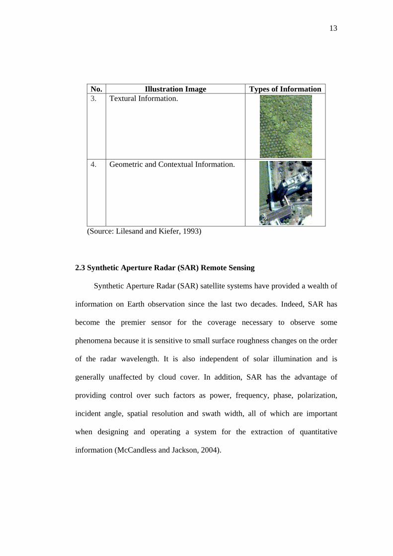
There are four main types of information contained in an optical image

that often utilized for image interpretation. The types and illustration are showed

in Table 2.1 below.

Table 2.1 Types of Information in Optical Image

No. Illustration Image Types of Information 1. Radiometric Information (brightness,

intensity, and tone).

2. Spectral Information (color, and hue).

13

No. Illustration Image Types of Information 3. Textural Information.

4. Geometric and Contextual Information.

(Source: Lilesand and Kiefer, 1993)

2.3 Synthetic Aperture Radar (SAR) Remote Sensing

Synthetic Aperture Radar (SAR) satellite systems have provided a wealth of

information on Earth observation since the last two decades. Indeed, SAR has

become the premier sensor for the coverage necessary to observe some

phenomena because it is sensitive to small surface roughness changes on the order

of the radar wavelength. It is also independent of solar illumination and is

generally unaffected by cloud cover. In addition, SAR has the advantage of

providing control over such factors as power, frequency, phase, polarization,

incident angle, spatial resolution and swath width, all of which are important

when designing and operating a system for the extraction of quantitative

information (McCandless and Jackson, 2004).

14

2.3.1 SAR Principles

SAR is the most common form of active microwave radar sensors. The

active radar sensors record the intensity of the transmitted microwave energy

backscattered to the sensor. In SAR imaging, microwave pulses are transmitted by

an antenna towards the earth surface. The microwave energy scattered back to the

spacecraft is measured. When microwaves strike a surface, the proportion of

energy scattered back to the sensor depends on many factors, such as physical

factors, geometric factors, the types of land cover, and microwave frequency,

polarization and incident angle.

The SAR makes use of the radar principle to form an image by utilizing

the time delay of the backscattered signals. Moreover, SAR capitalizes on the

motion of the space craft which has a limitation to carry a very long antenna to

emulate a large antenna from the small antenna it actually carries on board for a

high resolution imaging of the Earth surface (Matsuoka and Yamazaki, 2000).

 

Figure 2.5 Geometry’s Image for a Typical Strip-Mapping SAR Imaging System

(Source: Liew, 2001)

15

2.3.2 Microwave Frequency

The ability of microwave to penetrate clouds, precipitation, or land surface

cover depends on its frequency. Generally, the penetration power increases for

longer wavelength (lower frequency). The SAR backscattered intensity generally

increases with the surface roughness. In SAR imaging, the reference length scale

for surface roughness is the wavelength of the microwave. If the surface

fluctuation is less than the microwave wavelength, then the surface is considered

smooth. The short wavelength radar interacts mainly with the top layer of the

forest canopy while the longer wavelength radar is able to penetrate deeper into

the canopy to undergo multiple scattering between the canopy, trunks and soil

(McCandless and Jackson, 2004).

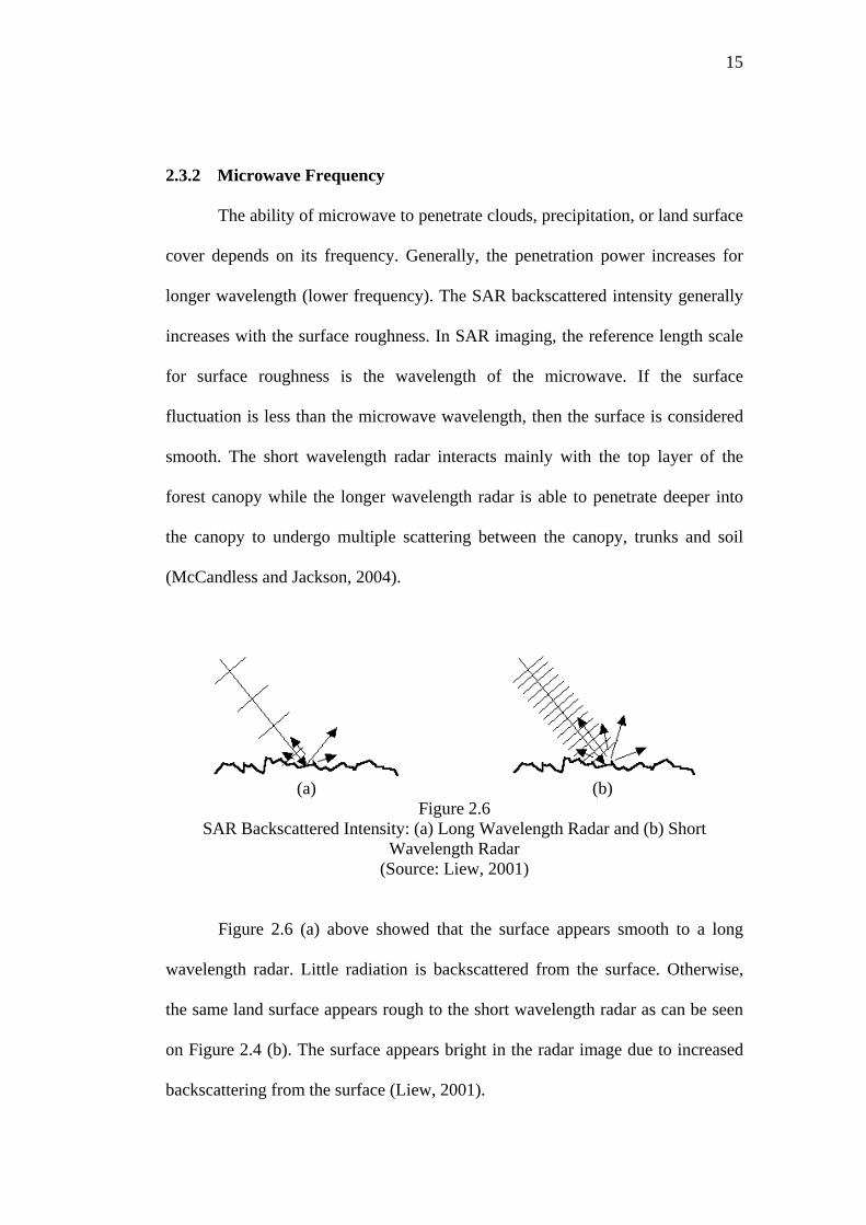
(a) (b) Figure 2.6

SAR Backscattered Intensity: (a) Long Wavelength Radar and (b) Short Wavelength Radar

(Source: Liew, 2001)

Figure 2.6 (a) above showed that the surface appears smooth to a long

wavelength radar. Little radiation is backscattered from the surface. Otherwise,

the same land surface appears rough to the short wavelength radar as can be seen

on Figure 2.4 (b). The surface appears bright in the radar image due to increased

backscattering from the surface (Liew, 2001).

16

2.3.3 Polarization Wave

The microwave polarization refers to the orientation of the electric field

vector of the transmitted beam with respect to the horizontal direction. If the

electric field vector oscillates along a direction parallel to the horizontal direction,

the beam is said to be “H” polarized. On the other hand, if the electric field vector

oscillates along a direction perpendicular to the horizontal direction, the beam is

“V” polarized. After interacting with the earth surface, the polarization state may

be altered. There are four possible polarization configurations for a SAR system,

namely “HH”, “VV”, “HV” and “VH”. It depends on the polarization states of the

transmitted and received microwave signals (McCandless and Jackson, 2004).

2.3.4 Incident Angles

The incident angle refers to the angle between the incident radar beam and

the direction perpendicular to the ground surface. The interaction between

microwaves and the surface depends on the incident angle of the radar pulse on

the surface. A small incident angle is optimal for detecting ocean waves and other

ocean surface features. While a larger incident angle may be more suitable for

other applications. For example, a large incident angle will increase the contrast

between the forested and clear cut areas. Acquisition of SAR images of an area

using two different incident angles will also enable the construction of a stereo

image for the area (Baumann, 2010).

17

2.3.5 SAR Signal Processing and Image Formation

In a SAR signal processor there are specific operations required to convert

a raw data set into an interpretable image. The raw SAR data is not an image since

point targets are spread out in range and in the along-track dimension. Figure 2.7

illustrates the raw data trace of a typical point-target as the beam moves in the

along-track or azimuth direction. As the radar moves by the target, the radar-to-

target range varies, forming the curved trace shown. This translation also

produces an along-track frequency/time trace in azimuth, induced by Doppler, and

range pulse encoding produces a somewhat similar time/frequency trace in range.

The SAR signal processor compresses this distributed target information in two

dimensions (range and along-track) to create the image (Baumann, 2010).

Figure 2.7 SAR Point Target Return

(Source: McCandless and Jackson, 2004)

18

Several computation techniques may be used to form a SAR image. One

method is to use Fourier spectrum estimation techniques, commonly implemented

through a “Fast Fourier Transform”. Time domain matched filters may also be

used. The choice is applications dependent and usually made based on

computational efficiencies. In summary, SAR image formation requires many rote

process and computation intensive signal processing of coherent radar return

phase histories (Curlander and McDonough, 1991).

2.3.6 Geometry and Speckle Characteristics of SAR Images

A SAR image has several characteristics that make it different with the

other image. The position and proportions of objects in the image can appear

distorted and also grain, due to the presence of many black and white pixels

randomly distributed throughout the image.

1. Slant Plane/ Ground Plane

Slant plane is the distance that measured along the line between the radar

and surface of the earth where the pulse travels. The distances were

converted from the delay time associated with a particular reflection. The

resolution in the ground plane image is coarser then the corresponding

slant plane image. To make a SAR image appear like a map, the sampling

along the slant plane must be converted to the ground plane. Slant to

ground range distortions are often small for the space-based SARs because

of the small variation in incident angle from the near side of the swath

(Liew, 2001).

19

2. Speckle Noise

Unlike optical images, radar images are formed by coherent interaction of

the transmitted microwave with the targets. Hence, it suffers from the

effects of speckle noise which arises from coherent summation of the

signals scattered from ground scatters distributed randomly within each

pixel. A radar image appears noisier than an optical image. The speckle

noise is sometimes suppressed by applying a speckle removal filter on the

digital image before display and further analysis. The vegetated areas and

the clearings appear more homogeneous after applying a speckle removal

filter to the SAR image (Liew, 2001).

(a) (b)

Figure 2.8 SAR Image Before and After Applying Speckle Noise Removal

(Liew, 2001)

2.3.7 Backscattered Radar Intensity

A single radar image is usually displayed as a grey scale image, such as

the one shown above. The intensity of each pixel represents the proportion of

20

microwave backscattered from that area on the ground which depends on a variety

of factors, such as types, sizes, shapes and orientations of the scatters in the target

area, moisture content of the target area, frequency and polarization of the radar

pulses, as well as the incident angles of the radar beam. The pixel intensity values

are often converted to a physical quantity called the backscattering coefficient or

normalized radar cross-section measured in decibel (dB) units with values ranging

from +5 dB for very bright objects to -40 dB for very dark surfaces (Liew, 2001).

2.3.8 Interpreting SAR Images

Interpreting a radar image is not a straightforward task. It very often

requires some familiarity with the ground conditions of the areas imaged. As a

useful rule of thumb, the higher the backscattered intensity, the rougher is the

surface being imaged.

Flat surfaces such as paved roads, runways or calm water normally appear

as dark areas in a radar image since most of the incident radar pulses are

commonly reflected away. Calm sea surfaces appear dark in SAR images.

However, rough sea surfaces may appear bright especially when the incidence

angle is small. Trees and other vegetation are usually moderately rough on the

wavelength scale. Hence, they appear as moderately bright features in the image.

The tropical rain forests have a characteristic backscatter coefficient of between -6

and -7 dB, which is spatially homogeneous and remains stable in time. For this

reason, the tropical rainforests have been used as calibrating targets in performing

radiometric calibration of SAR images (Lilesand and Kiefer, 1993).

21

Very bright targets may appear in the image due to the corner-reflector or

double-bounce effect where the radar pulse bounces off the horizontal ground (or

the sea) towards the target, and then reflected from one vertical surface of the

target back to the sensor. Examples of such targets are ships on the sea, high-rise

buildings and regular metallic objects such as cargo containers. Built-up areas and

many man-made features usually appear as bright patches in a radar image due to

the corner reflector effect (Lilesand and Kiefer, 1993).

2.4 Image Processing and Analysis

Image processing and analysis techniques have been developed to aid the

interpretation of remote sensing images and to extract as much information as

possible from the images. The choice of specific techniques or algorithms to use

depends on the goals of project. Some procedures commonly used in analyzing or

interpreting remote sensing images are described below.

1. Pre-Processing

Prior to data analysis, initial processing on the raw data is usually carried out

to correct for any distortion due to the characteristics of the imaging system

and imaging conditions. Depending on the user's requirement, some standard

correction procedures may be carried out by the ground station operators

before the data is delivered to the end-user. These procedures include

radiometric correction to correct for uneven sensor response over the whole

image and geometric correction to correct for geometric distortion due to

Earth's rotation and other imaging conditions (such as oblique viewing). The

22

image may also be transformed to conform to a specific map projection

system. Furthermore, if accurate geographical location of an area on the

image needs to be known, ground control points (GCP’s) are used to register

the image to a precise map (geo-referencing) (ITT, 2006).

2. Image Enhancement

In the above unenhanced image, a bluish tint can be seen all-over the image,

producing a hazy appearance. This hazy appearance is due to scattering of

sunlight by atmosphere into the field of view of the sensor. This effect also

degrades the contrast between different land covers.

It is useful to examine the image Histograms before performing any image

enhancement. The x-axis of the histogram is the range of the available digital

numbers, for example from 0 to 255. The y-axis is the number of pixels in the

image having a given digital number.

The image can be enhanced by a simple linear grey-level stretching. In this

method, a level threshold value is chosen so that all pixel values below this

threshold are mapped to zero. An upper threshold value is also chosen so that

all pixel values above this threshold are mapped to 255. All other pixel values

are linearly interpolated to lie between 0 and 255. The lower and upper

thresholds are usually chosen to be values close to the minimum and

maximum pixel values of the image (ITT, 2006).

23

3. Image Classification

Different land cover types in an image can be discriminated using some

image classification algorithms using spectral features, such as the brightness

and the color information contained in each pixel. The classification

procedures can be “supervised” or “unsupervised”.

In supervised classification, the spectral features of some areas of known land

cover types are extracted from the image as the training areas. Every pixel in

the whole image is then classified as belonging to one of the classes

depending on how close its spectral features are to the spectral features of the

training areas. In unsupervised classification, the computer program

automatically groups the pixels in the image into separate clusters, depending

on the spectral features (IDRISI, 2009).

4. Image Segmentation

Segmentation is a process to divide an image into regions or objects. The

segmentation module generates an image of segments where pixels identified

within a segment share a homogeneous spectral similarity. Across space and

over all input bands, a moving window assesses this similarity and segments

are defined according to a user-specified similarity threshold. The smaller the

threshold, then the segments will be more homogeneous. A larger threshold

will cause a more heterogeneous and generalized segmentation result.

The segmentation process consists of three procedures. First, for each input

image, a corresponding variance image is created using a user-defined filter.

24

The pixels values within the variance image are then treated like elevation

values within a digital elevation model. Pixels are grouped into one watershed

if they are within one catchment. Each watershed is given a unique integral

value as its ID. The watersheds or image segments are then merged to form

new segments (IDRISI, 2009).

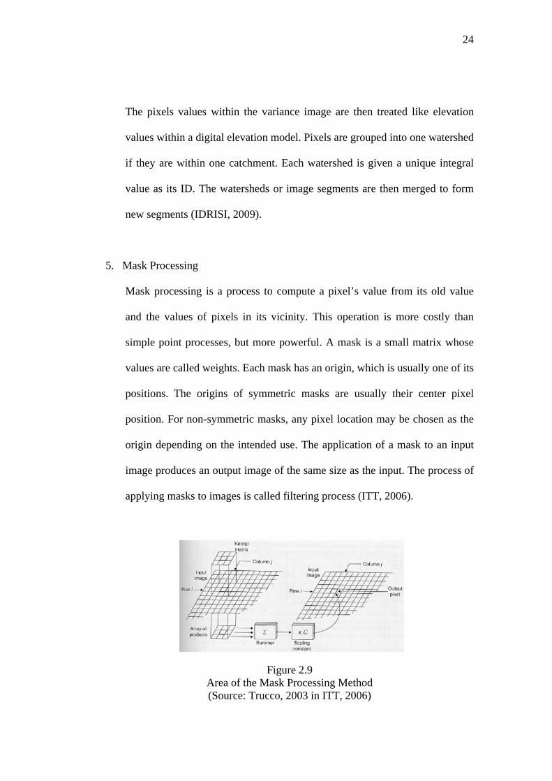
5. Mask Processing

Mask processing is a process to compute a pixel’s value from its old value

and the values of pixels in its vicinity. This operation is more costly than

simple point processes, but more powerful. A mask is a small matrix whose

values are called weights. Each mask has an origin, which is usually one of its

positions.  The origins of symmetric masks are usually their center pixel

position. For non-symmetric masks, any pixel location may be chosen as the

origin depending on the intended use. The application of a mask to an input

image produces an output image of the same size as the input. The process of

applying masks to images is called filtering process (ITT, 2006).

Figure 2.9 Area of the Mask Processing Method (Source: Trucco, 2003 in ITT, 2006)

25

6. Vegetation Index

Since vegetation has high NIR reflectance but low red reflectance, vegetated

areas will have higher values compared to non-vegetated areas. Another

commonly used vegetation index is the Normalized Difference Vegetation

Index (NDVI) computed by the equation below:

NDVI = (NIR - Red) / (NIR + Red) (2.1)

In the NDVI map shown above, the bright areas are vegetated while the non-

vegetated areas (buildings, clearings, river, and sea) are generally dark. Note

that the trees lining the roads are clearly visible as grey linear features against

the dark background. The NDVI band may also be combined with other

bands of the multispectral image to form a color composite image which

helps to discriminate different types of vegetation (Suppasri, 2012)

2.5 Advanced Land Observing Satellite (ALOS) Imagery

The Advanced Land Observing Satellite (ALOS) was launch on 24 January

2006. ALOS has three remote-sensing instruments, the Panchromatic Remote-

sensing Instrument for Stereo Mapping (PRISM) for digital elevation mapping,

the Advanced Visible and Near Infrared Radiometer type 2 (AVNIR-2) for

precise land coverage observation, and the Phased Array type L-band Synthetic

Aperture Radar (PALSAR) for day-and-night and all-weather land observation

(Shimada, 2007).

26

 

Figure 2.10 Advanced Land Observing Satellite (ALOS)

(Source: Shimada, 2007)

2.5.1 AVNIR-2

The on-board AVNIR-2 is a high resolution imaging spectrometer

operating in the visible and NIR spectrum and successor to AVNIR on-

board the Advances Earth Observation Satellite (ADEOS). It mainly

observes land and coastal areas in visible and near-infrared bands.

AVNIR-2 data are available in Level １A, Level 1B1 and Level 1B2,

which are generated by applying radiometric and geometric corrections to

the acquired data (ESA, 2007).

Table 2.2 Characteristics and Specifications of the AVNIR-2 Instruments

Items Characteristics

Instrument illustration

Number of Bands 4 Wavelength Band1 : 0.42 - 0.50 micrometers

Band2 : 0.52 - 0.60 micrometers Band3 : 0.61 - 0.69 micrometers Band4 : 0.76 - 0.89 micrometers

27

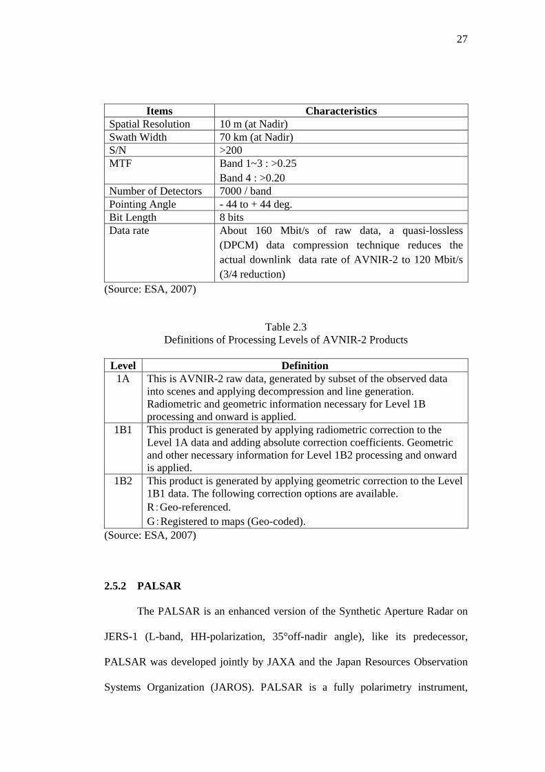
Items Characteristics Spatial Resolution 10 m (at Nadir) Swath Width 70 km (at Nadir) S/N >200 MTF Band 1~3 : >0.25

Band 4 : >0.20 Number of Detectors 7000 / band Pointing Angle - 44 to + 44 deg. Bit Length 8 bits Data rate About 160 Mbit/s of raw data, a quasi-lossless

(DPCM) data compression technique reduces the actual downlink data rate of AVNIR-2 to 120 Mbit/s (3/4 reduction)

(Source: ESA, 2007)

Table 2.3 Definitions of Processing Levels of AVNIR-2 Products

Level Definition 1A This is AVNIR-2 raw data, generated by subset of the observed data

into scenes and applying decompression and line generation. Radiometric and geometric information necessary for Level 1B processing and onward is applied.

1B1 This product is generated by applying radiometric correction to the Level 1A data and adding absolute correction coefficients. Geometric and other necessary information for Level 1B2 processing and onward is applied.

1B2 This product is generated by applying geometric correction to the Level 1B1 data. The following correction options are available. R：Geo-referenced. G：Registered to maps (Geo-coded).

(Source: ESA, 2007)

2.5.2 PALSAR

The PALSAR is an enhanced version of the Synthetic Aperture Radar on

JERS-1 (L-band, HH-polarization, 35°off-nadir angle), like its predecessor,

PALSAR was developed jointly by JAXA and the Japan Resources Observation

Systems Organization (JAROS). PALSAR is a fully polarimetry instrument,

28

operating in fine-beam mode with single polarization (HH or VV), dual

polarization (HH+HV or VV+VH), or full polarimetry (HH+HV+VH+VV). It

also features wide-swath ScanSAR mode, with single polarization (HH or VV).

The center frequency is 1270 Mhz (23.6 cm), with a 28 MHz bandwidth in fine

beam single polarization mode, and 14 MHz in the dual-, quad-pol and ScanSAR

modes. The off-nadir angle is variable between 9.9° and 50.8° (at mid-swath),

corresponding to a 7.9 - 60.0° incidence angle range. In 5-beam ScanSAR mode,

the incidence angle range varies from 18.0° to 43.0° (Rosenqvist, et. al., 2004).

Figure 2.11 PALSAR Observation Characteristics

(Source: Rosenqvist, et. al., 2004)

Table 2.4 ALOS/PALSAR Characteristics

Mode Fine ScanSAR Polarimetric (Experimental

mode)*1 Center frequency

1270 MHz(L-band)

Chirp bandwidth

28MHz 14MHz 14MHz,28MHz 14MHz

29

Mode Fine ScanSAR Polarimetric (Experimental

mode)*1

Mode

Polarization HH or VV

HH+HV or

VV+VH

HH or VV HH+HV+VH+VV

Incident angle

8 to 60deg.

8 to 60deg.

18 to 43deg. 8 to 30deg.

Range Resolution

7 to 44m 14 to 88m 100m (multi look)

24 to 89m

Observation swath

40 to 70km

40 to 70km

250 to 350km 20 to 65km

Bit length 5 bits 5 bits 5 bits 3 or 5bits Data rate 240Mbps 240Mbps 120Mbps,

240Mbps 240Mbps

NE sigma zero *2

< -23dB (Swath Width 70km)

< -25dB (Swath Width 60km)

< -25dB < -29dB

S/A *2,*3 > 16dB (Swath Width 70km)

> 21dB (Swath Width 60km)

> 21dB > 19dB

Radiometric accuracy

scene: 1dB / orbit: 1.5 dB

(Source: Rosenqvist, et. al., 2004)

2.6 Tsunami

A tsunami is the Japanese word for the large harbor wave which is a series

of large water waves that produced by a sudden vertical displacement of water.

While rare, tsunamis have a potential to cause considerable loss of life and injury

as well as widespread damage to the natural and built environments (Doocy, et. al,

2013). One of the historical tsunami events, the 2010 Chilean tsunami earthquake

left 521 dead, 76 missing, according to official figures, and displaced an estimated

2 million people. Almost eight months after the combined events in Talcahuano,

30

300 miles south of the capital Santiago, once a bustling port is still paralyzed,

houses are destroyed and trade through the port barely a trickle (ITIC, 2010).

2.6.1 Definition and Characteristics of Tsunami

Tsunami is officially defined as a wave train, or series of waves, generated

in a body of water by an impulsive disturbance that vertically displaces the water

column. In general, anything that is capable of moving large water masses can

cause a tsunami. Various sources as earthquakes, landslides, volcanic eruptions,

explosions, and even the impact of cosmic bodies, such as meteorites, can

generate tsunamis (Doocy, et. al., 2013).

Aquatic earthquakes are the most common cause in generating tsunamis.

A tsunami which is generated by earthquakes develop when tectonic plates, either

deep sea, continental shelf, or coastal, move abruptly in a vertical direction, and

the overlying water is displaced. Waves created by these disturbances move in an

outward direction, away from the source. In deep waters, the surface disturbances

move in and outward direction, away from the source. It is also relatively

unnoticeable and may only be felt as a gentle wave. As the wave approaches

shallow waters along the coast, it rises above the surface related to the amplitude

of the underwater waves. The speed of the tsunami diminishes and the height of

the wave increases as it reaches the shore line. The extent of inundation that

occurs is largely dependent on local topography, where in low lying areas

flooding can be extensive and can reach far inland disrupting even non-coastal

communities (Keller and Blodget, 2008).

31

 

Figure 2.12 A Tsunami which is Generated by Earthquakes

(Source: Meijde, 2006)

There are several specific characteristics related to tsunamis that make it

clearly distinguishable from other types of waves (Meijde, 2006):.

1. Tsunamis can appear as a falling or rising tide, waves or bore

2. Tsunamis can last for several hours.

3. A tsunami consists of several wave trains following each other.

4. A pattern of high water levels is alternated with low water levels.

2.6.2 The 2010 Chile Tsunami Earthquake

Chile is one of the seismically most active countries in the world with an

earthquake of magnitude 8 or larger (M ≥ 8) occurring every 10 years. The most

recent event was an earthquake with moment magnitude (Mw) 8.8 which was

occurred on the February 27th, 2010 at 3:34 hours, local time in Chile (06:34

hours UTC). The epicenter region of the event is located in the Chile-Peru trench

between the 35�S and 37�S, in the so called Concepción-Constitución seismic gap,

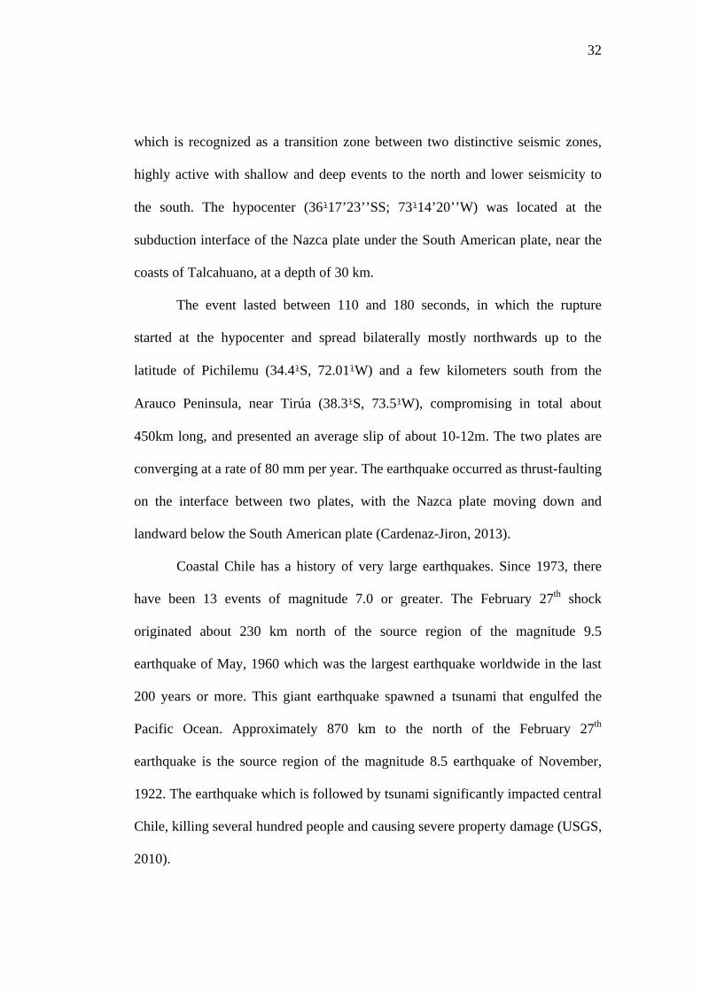
32

which is recognized as a transition zone between two distinctive seismic zones,

highly active with shallow and deep events to the north and lower seismicity to

the south. The hypocenter (36�17’23’’SS; 73�14’20’’W) was located at the

subduction interface of the Nazca plate under the South American plate, near the

coasts of Talcahuano, at a depth of 30 km.

The event lasted between 110 and 180 seconds, in which the rupture

started at the hypocenter and spread bilaterally mostly northwards up to the

latitude of Pichilemu (34.4�S, 72.01�W) and a few kilometers south from the

Arauco Peninsula, near Tirúa (38.3�S, 73.5�W), compromising in total about

450km long, and presented an average slip of about 10-12m. The two plates are

converging at a rate of 80 mm per year. The earthquake occurred as thrust-faulting

on the interface between two plates, with the Nazca plate moving down and

landward below the South American plate (Cardenaz-Jiron, 2013).

Coastal Chile has a history of very large earthquakes. Since 1973, there

have been 13 events of magnitude 7.0 or greater. The February 27th shock

originated about 230 km north of the source region of the magnitude 9.5

earthquake of May, 1960 which was the largest earthquake worldwide in the last

200 years or more. This giant earthquake spawned a tsunami that engulfed the

Pacific Ocean. Approximately 870 km to the north of the February 27th

earthquake is the source region of the magnitude 8.5 earthquake of November,

1922. The earthquake which is followed by tsunami significantly impacted central

Chile, killing several hundred people and causing severe property damage (USGS,

2010).

33

Figure 2.13 The 2010 Tsunami Earthquake Location in Chile

(Source: USGS, 2010)

2.7 The Use of Remote Sensing Technology for Tsunami Disaster Analysis

It is generally difficult to make short-term assessment of the impact of a

major natural disaster as the consequences may vary according to the spatial scale,

the time interval leading up to and following the disasters, as well as other

variable, which together make it necessary to have an enough time frame and a

large amount of information from a broad number of areas in order to perform an

accurate analysis. In this regard, the use of remote sensing provides a view of the

Earth’s surface at different scales of observation, thus providing greater detail and

achieving more precise analysis (Stramondo et. al., 2008).

34

Satellite observation scales range from kilometers to centimeters, thus

making it possible to gauge the extent of damage caused by natural events, in

particular, earthquakes and tsunamis. In fact, with a single image it is possible to

estimate the damage caused by these phenomena immediately after the natural

event. However, it is always necessary to compare this information with

additional data in order to better quantify the damage caused by the different types

of natural disasters that might occur in a particular area (Stramondo et. al., 2008).