CHAPTER I INTRODUCTION - Shodhgangashodhganga.inflibnet.ac.in/bitstream/10603/33882/1/... · 2018-07-02 · 1 CHAPTER I INTRODUCTION In this chapter concept, terminologies and symbols

1

CHAPTER I

INTRODUCTION

In this chapter concept, terminologies and symbols of acceptance sampling

relevant to this dissertation are explained.

American National Standards Institute/ American Society for Quality Control

standard A2 (1987) defines acceptance sampling is the methodology which deals with the

procedures for decision to accept or reject manufactured product based on the inspection

of samples. According to Dodge (1969) Statistical Quality Control has been defined as

“the concept of protecting the consumer from getting unacceptable defective material and

encouraging the producer towards process quality control by varying the quality and

severity of acceptance inspection, in direct relation to the importance of characteristics

inspected and has inverse relation to the goodness of the quality level as indicated by

these inspections”.

According to Dodge (1969) the major areas of Acceptance Sampling are:

1) Lot-by-Lot sampling by the method of attributes, in which each unit in a sample is

inspected on a go-not-go basis for one or more characteristics;

2) Lot-by-Lot sampling by the method of variables, in which each unit in a sample is

measured for a single characteristic such as weight or strength;

3) Continuous sampling for a flow of units by the method of attributes; and

4) Special purpose plans including chain sampling, skip-lot sampling, small sample

plans etc.

A sampling plan prescribes the sample size and the criteria for accepting, rejecting

or taking another sample to be used in inspecting a lot. This thesis establishes procedures

for new sampling plans, schemes/systems, various theorems and empirical relations.

Certain concepts, terminology and notations relevant to the study are well discussed.

Tables and graphs are also given for each plan separately in the respective chapters. Most

of the definitions are taken from American National Standards Institute/ American

Society for Quality Control (ANSI /ASQC) standard A2 (1987).

Please purchase PDF Split-Merge on www.verypdf.com to remove this watermark.

2

This dissertation is concerned with development of various methods for designing

sampling plans based on range of quality, instead of point- wise description of quality by

invoking novel approach called Quality Interval Sampling Procedure. This method seems

to be versatile and adopted to the elementary production process where the stipulated

quality level is advisable to fix at a later stage and provides a new concept meant for

designing sampling plans involving through quality levels. This thesis also explains

procedures for various special purpose plans with Quality Interval Sampling Plan (QISP)

and Quality Interval Bayesian Sampling Plan (QIBSP) with given set of conditions or

indices specified towards construction and selection of plans. The main purpose of this

thesis are:

• To construct Quality Interval Sampling Plan (QISP) in which the designing of

plans indexed through Quality Regions.

• To construct Quality Interval Bayesian Sampling Plan (QIBSP) in which

construction and selection of plans based on range of quality.

Bayesian Approach

Bayesian Acceptance Sampling Approach is associated with the utilization of

prior process history for the selection of distributions (viz., Gamma Poisson, Beta

Binomial) to describe the random fluctuations involved in Acceptance Sampling.

Bayesian sampling plans requires the user to specify explicitly the distribution of

defectives from lot to lot. The prior distribution is the expected distribution of a lot

quality on which the sampling plan is going to operate. The distribution is called prior

because it is formulated prior to the taking of samples. The combination of prior

knowledge, represented with the prior distribution, and the empirical knowledge based on

the sample leads to the decision about the lot quality construction.

• It consists of minimizing average (expected) costs, including inspection,

acceptance and rejection costs.

• Bayesian statistics is useful to sampling issues

• It takes into account prior information in the sampling set up

• It can update information through the Bayes formula to modify/adapt the sampling

stringency according to the latest results

• It removes uncertainty on parameter of interest when decision making is carried


3

Chapter I provides an introduction about Statistical Quality Control specifically on

Acceptance Sampling. The introductions of the classical and Bayesian Sampling plans

constructed in this thesis are well explained in the chapter I. This chapter consists of

twelve sections.

The section wise contents are indicated as below:

Section 1.1. Deals with terms, notations and terminologies in connection with results

presented under the entire thesis.

Section 1.2. Review on Single Sampling plan, Special Type Double Sampling Plan and

Repetitive Group Sampling Plan.

Section 1.3. Brief review on One Plan Suspension System and Two Plan System.

Section 1.4. A brief survey on Chain Sampling and Skip-lot Sampling Plans.

Section 1.5. Review on Bagchi’s Two Level Chain Sampling and Modified Two Level

Chain Sampling Plans.

Section 1.6. Review on Multiple Deferred Sampling and Double Sampling Plans.

Section 1.7. Brief Review on Quick Switching System proposed by Romboski.

Section 1.8. Review on Bayesian Repetitive Group Sampling Plan, Bayesian Chain

Sampling Plan and Bayesian Skip-lot Sampling Plan

Section 1.9. Review on Bayesian Multiple Deferred Sampling Plan

Section 1.10. Review on Bayesian Quick Switching System and Bayesian One Plan

Suspension System.

Section1.11. Review on Construction of Plans involving through minimization approach

Section1.12. Review on Designing of Plans involving through Quality Regions


4

SECTION 1.1: BASIC TERMINOLOGIES AND NOTATIONS

Certain Concepts and terminologies of acceptance sampling are explained in this

section.

Sampling Plan

ANSI/ASQC Standard A2 (1987) defines an acceptance sampling plan is a

“specific plan that states the sample rules to be used with the associated acceptance and

rejection criteria”. In acceptance sampling plan the operating characteristics directly

follows from the parameters specified which are uniquely determined.

Sampling Scheme

ANSI/ASQC Standard A2 (1987) defines acceptance sampling scheme as a

“specific set of procedures which usually consists of acceptance sampling plan in which

lot size, sample sizes and acceptance criteria or the amount of 100 percent inspection and

sampling are related”.

Sampling System

Hill (1962) has described the difference between the sampling plan and sampling

scheme. According to Hill (1962) a sampling scheme “is a whole set of sampling plans

and operations included in the standard describes the overall strategy specifying the way

in which the sampling plans are to be used”. Stephens and Larson (1967) have described a

sampling system “as an assigned grouping of two or three sampling plans and the rules

for using these plans for sentencing lots to achieve a blending which is advantageous

feature for these sampling plans”

Cumulative and Non-Cumulative Sampling plans

Stephens (1966) defines non-cumulative sampling plan as one which uses the

current sample information from the process or current product entity in making decisions

about the process or product quality. Single and Double sampling plans are examples for

such non-cumulative sampling plan. Cumulative results sampling inspection is one which

uses the current and past information from the process towards making a decision about

the process. Chain sampling plan of Dodge (1955) is an example for a cumulative results

sampling plan.


5

Inspection

ANSI/ASQC Standard A2 (1987) defines the term inspection as “activities”, such

as measuring, examining, testing, gauging one or more characteristics of a product and /

or service and comparing these with specified requirements to determine conformity. A

sampling scheme or sampling system may contain three types of inspections namely

normal, tightened and reduced inspection. ANSI/ ASQC Standard A2 (1987) defines as

follows:

Inspection, Normal

Inspection that is used in accordance with an acceptance sampling scheme when a

process is considered to be operating at or slightly better than its acceptable quality level.

Inspection, Tightened

A feature of a sampling scheme using stricter acceptance criteria than those used

in normal inspection.

Inspection, Reduced

A feature of a sampling scheme, permitting smaller sample sizes than used in

normal inspection.

Operating Characteristic (OC) Curve

Associated with each sampling plan, there is an operating characteristic curve,

which describes clearly the performance of the sampling plan against good and bad

quality. The interrelationship of the risks, probabilities and the qualities of a given

sampling plan can be shown graphically through an operating characteristics curve. The

OC curve gives are generally classified under Type A and Type B.ANSI /ASQC standard

(1987) defines them as follows:

Type A OC Curve for Isolated or unique Lots, or a lot from an Isolated sequences:

“A curve showing, for a given sampling plan, the probability of accepting a lot as

a function of the lot quality”

Sampling from an individual (or isolated) lot, with a curve showing probability of

lots, which will be accepted when plotted against lot proportion defective.


6

Type B OC Curve for a continuous stream of Lots:

Sampling from a process, with a curve showing proportion of lots, which will be

accepted when plotted against process proportion defective.

According to Schilling (1982), the conditions under which Binomial, Poisson and

Hyper geometric models can be used are follows:

Binomial Model

This model is exact for the case of non-conforming units under Type B situations.

The model can also be used under Type A situations for the case of non-conforming units

whenever 10.0≤N

n, where n and N are the sample and lot sizes respectively.

Poisson Model

This model is exact for the case of non-conformities under both Type B and Type

A situations. Under Type A situations, for the case of non-conformities units, Poisson

model can be used whenever 10.0≤N

n, n is large and p is small such that 5<np .

Under Type B situations, for the case of non-conformities units this model can be used

whenever n is large and p is small such that 5<np .

Hypergeometric Model

This is exact model for the case of non-conforming units under Type A situations

and is useful for isolated lots.

Gamma- Poisson Distribution

In Bayesian inference, the conjugate prior for the rate parameter p of the Poisson

distribution is the Gamma distribution. Let ),(~ tsGammap denote that p is

distributed according to the Gamma density w parameterized in terms of a shape

parameter p and an inverse scale parameter t.

0 ,0, ),(/),;()( 1 >>Γ= −− ptsstpetspworGamma sspt

= 0 Otherwise


7

Then, given the same sample of n measured values ki as before, and a prior of

Gamma(s, t), the posterior distribution is

),(~1

ntksGammapn

i

i ++ ∑=

The posterior mean E[p] approaches the maximum likelihood estimate ∧

MLEp in

the limit as 0,0 →→ ts .The posterior predictive distribution of additional data is a

Gamma Poisson distribution (i.e.negative binomial) distribution.

Beta- Binomial Distribution

Let x be the outcome of n Bernoulli trials with a fixed probability p, and let the

corresponding binomial probability be denoted as

xnx

x

n qpCpnxb −=),,(

Assuming that p has a prior distribution with density ),( pw the marginal

distribution of x, the mixed binomial distribution is given as

∫=1

0

)(),,(),( dppwpnxbnxbw

Average Sample Number

ANSI / ASQC A2 standard (1987) defines ASN as “the average number of sample

units per lot used for making decisions (acceptance or non-acceptance)”. A plot of ASN

against p is called the ASN curve.

Average Outgoing Quality (AOQ) and Average Outgoing Quality Limit (AOQL)

ANSI/ASQC Standard A2 (1987) defines AOQ as “the expected quality outgoing

product following the use of an acceptance sampling plan for a given value of incoming

product quality”. Similarly for a given sampling plan, AOQL is defined as “the maximum

AOQ over all possible levels of incoming quality”. Policies adopted for replacing and

removing non-conforming units in sampling and screening phases causes the expressions

for AOQ to vary. Beainy and Case (1981) have given expressions for AOQ over different

policies adopted for single and double sampling attribute plans. Further AOQ is


8

approximated as )(. pPap . The assumptions underlying this expressions is that for all

accepted lots, the average fraction non-conforming is assumed to be p and for all the

rejected lots the entire units are being screened and non-conforming units are replaced

with good units. It is further assumed that the sampling fractionN

n is very small and can

be ignored. A plot of AOQ against p is called the AOQ curve.

Average Total Inspection (ATI)

According to ANSI/ASQC standard A2 (1987) ATI is “the average number of

units inspected per lot based on the sample size for accepted lots and all inspected units in

not accepted lots’. ATI is not applicable whenever testing is destructive. A plot of ATI

against p is called ATI curve for the plan.

Acceptable Quality Level (AQL)

ANSI/ASQC Standard A2 (1987) defines AQL as “the maximum percentage or

proportion of variant units in a lot or batch, for the purpose of acceptance sampling can be

considered as a satisfactory process average”.

Producer’s Risk ( α )

The producer’s risk α is the probability that a good lot will be rejected by the

sampling plan. The risk is stated in conjunction with a numerical definition of maximum

quality level that may pass through the plan often called Acceptable Quality Level.

Usually considered with α = 0.05

Limiting Quality Level (LQL)

ANSI/ASQC Standard A2 (1987) defines LQL as “the percentage or proportion of

variant units in a batch or lot, for the purpose of acceptance sampling, the consumer

wishes the probability of acceptance to be restricted to a specified low value”.

Consumer’s Risk (β)

The consumer’s risk β is the probability that the bad lot will be accepted by the

sampling plan. The risk is stated in conjunction with numerical definition of rejectable

quality such as lot tolerance percent defective.


9

Indifference Quality Level (IQL)

The percentage of variant units in a branch of lot, for purposes of Acceptance

sampling, the probability of acceptance to be restricted to a specific value namely 0.50.

The point (IQL, 0.50) on the OC curve is also called as “Point of control”.

Maximum Allowable Percent Defective (MAPD)

The point on the OC curve at which decent is steepest, called the point of

inflection. The proportion non-conforming corresponding to the point of inflection on the

OC curve is interpreted as maximum allowable percent defective.

Maximum Allowable Average Outgoing Quality (MAAOQ)

The MAAOQ of a sampling plan is designated as the Average Outgoing Quality

(AOQ) at the MAPD. Then

*)(. ppatpPpMAAOQ a ==

This can be rewritten as

)( ** pPapMAAOQ =

Crossover Point ( cp )

Crossover point is the point on the composite OC- curve of any two plan system

that is located exactly halfway between the normal and tightened OC-curves. This is the

point at which the two levels of inspection make an equal contribution to the composite

OC- function. Romboski (1969) has defined this point and referred as the crossover point

(COP) and denoted as cp .

Crossover Maximum Allowable Average Outgoing Quality (COMAAOQ)

The Crossover Maximum Allowable Average Outgoing Quality (COMAAOQ) is

defined as the Crossover Average Outgoing Quality (COAOQ) at the COMAPD. That is,

cppatCOAOQCOMAAOQ *== .

This can be rewritten as )(. ** cc pPapCOMAAOQ =


10

Terminologies related to Bayesian Acceptance Sampling Plan

While comparing the concepts and terminologies of Bayesian acceptance

sampling plans with conventional acceptance sampling plans, all concepts remains the

same except that Bayesian sampling plans takes into account the past history of the lot.

Hence in order to differentiate the terminologies between them, a slight modification has

been made that the term “overall” has been made to some of the terms pertaining to

conventional sampling plans. The modification made to the Bayesian Sampling Plan

terminologies defines that the past history of the lots has been taken in to account as prior

distribution for the construction of sampling plans. It is listed as below:

• OAOQAOQ ≈ (Overall Average Outgoing Quality)

• OAOQLAOQL ≈ (Overall Average Outgoing Quality Limit)

• )()( ** µnMAAPDnpMAPD ≈ (Maximum Allowable Average Percent Defective)

• MAOAOQMAAOQ ≈ ( Maximum Allowable Overall Average Outgoing

Quality)

• )()( 11 µnAQLnpAQL ≈

• )()( 22 µnLQLnpLQL ≈

Designing of sampling plans

Under designing a sampling plan, one has to accomplish a number of different

purposes. According to Hamaker (1960), the important ones are:

1) To strike a proper balance between the consumer requirements, the producer’s

capabilities, and inspectors capacity.

2) To separate a bad lot from good.

3) Simplicity of procedures and administration,

4) Economy in number of observations towards inspection,

5) To reduce the risk of wrong decisions with increasing lot size,

6) To use accumulated sample data as a valuable source of information,

7) To exert pressure on the producer or supplier when the quality of the lots received

is unreliable or not up to the standard,

8) To reduce sampling when the quality is reliable and satisfactory,

9) Hamaker(1950) also noted that these aims are partly conflicting and all of them

cannot be simultaneously be realized.


11

Case and Keats (1982) have classified the selection of attribute sampling plan as in the

following table:

Sampling Plan Design Methodologies

Methodologies Risk Based Economically Based

Non Bayesian 1 2

Bayesian 3 4

In this dissertation, sampling plan design of category 1 and 3 (that is risk based

non-Bayesian approach and risk based Bayesian approach) is alone considered.

According to Case and Keats (1982), only the traditional category 1, sampling design is

applied by the vast majority of quality control practitioners due to their wider availability

and ease for applications.

According to Peach (1947), the following are some of the major types of designing

plans, which are classified according to types of protection:

1. The plan is specified by requiring the OC curve to pass through (or nearly

through) two fixed points. In some cases it may be possible to impose certain

additional conditions. The two points generally selected are )1,( 1 α−p and ),( 2 βp

where

α−11 porp = the quality level that is considered to be good so that the producer

expects lots of 1p quality to be accepted most of the time;

βporp2 = the quality level that is considered to be poor so that the consumer

expects lots of 2p quality to be rejected most of the time;

α = the producer’s risk of rejecting 1p quality;

β = the consumer’s risk of accepting 2p quality.

The tables provided by Cameron (1952) is an example for this type of designing.

Schilling (1982) considered the term 1p as the Producer’s Quality Level (PQL) and

2p as the Consumers Quality Level (CQL). Earlier literature calls 1p as the

Acceptable Quality Level and 2p as the Limiting Quality Level (LQL or LQ) or

Rejectable Quality Level (RQL) or Lot Tolerance Proportion Defective (LTPD).


12

Peach and Littauer (1946) have defined a ratio 1

2

p

p associated with specified values of

α andβ are assumed to take 0.05 and 0.10 respectively.

2. The plan is specified by fixing one point only through which the OC curve is

required to pass and setting up one or more conditions, not explicitly in terms of

the OC curve. Dodge and Romig (1959) LTPD tables is an example for this type

of designing.

3. The plan is specified by imposing upon the OC curve two or more independent

conditions none of which explicitly involves the OC curves. Dodge and Romig

(1959) AOQL tables is an example for this type of designing.

Designing Plans for Specified IQL

Hamaker (1950a) considered two important features of the OC curves namely the

place where the OC curve shows its steeper descent and the degree of its steepness, as the

basis for two indices namely , the IQL ( 0p ) and the relative slope of the OC curve at ( 0p ,

0.5) denoted as 0h , which may be used to design any sampling plan. Hamaker (1950b)

has given simple empirical relations existing between the sample size and the acceptance

number; between the parameters 0p and 0h under the conditions for application of

Poisson, Binomial and Hyper geometric models for single sampling attributes plan.

Soundararajan and Muthuraj (1985) have given procedures and tables for designing single

sampling attribute plans for specified 0p and h0.

Designing plans for specified MAPD

The proportion non- conforming corresponding to the inflection point of the OC

curve denoted by *p and interpreted as Maximum Allowable Percent Defective (MAPD)

by Mayer (1967) used the quality standard along with some other condition for the

selection of sampling plans. The relative slope of the OC curve at this point denoted as *h ,

also be used to fix the discrimination of the OC curve of any sampling plan. The

desirability of developing a set of sampling plan indexed by *p has been explained by

Mandelson (1962) and Soundararajan (1971). Sampling plan can be selected for given


13

*p and K *

(p

pK T= , Tp is the point at which the tangent line at the inflection point of

the OC curve cuts the p -axis) the (inverse) measure of discrimination or with *h , the

relative slope of the OC curve at *p . Soundarajan and Muthuraj (1985) provided the

procedures and tables for designing single sampling plan for given *p and *h .

Unity Value Approach

This approach is used only under the conditions for application of Poisson model for

the OC curve. Duncan (1986) and Schilling (1982) noted that the assumption of Poisson

model permits to consider the OC function of all attribute sampling plans simply as a

function of the product np but not on the sample size n and submitted quality p

individually for given acceptance and rejection numbers. This implies that the OC

function remains the same for various combinations of n and p provided their product is

the same for given acceptance and rejection numbers. As a result one can provide

compact tables for the selection of sampling plans as only one parameter np need be

considered in place of two parameters n and p . The primary advantage of the unity

value approach is that plans can be easily obtained and necessary tables constructed.

Cameron (1952) has used this approach for designing single sampling plans.

Search Procedure

In this approach the parameters of a sampling plan are chosen by trial and error

with varying the parameters in a uniform fashion depending upon the properties of OC

function. An example for this approach is the one followed by Gunether (1969, 1970)

while determining the parameters of single and double sampling plans, under the

conditions for the application of Binomial, Poisson and Hyper geometric models for OC

curve. The advantage of search procedure is that the sample size need not be rounded.

The disadvantage of this procedure is that obtaining parameters for plans need elaborate

computing facilities.


14

Designing Approaches adopted in this thesis

The various sections presented in this study are :

• Designing of Sampling Plans using Quality Regions

• Designing of Sampling Plan using Tangent Angle

• Designing of Sampling Plan using Minimum Sum of Risk

• Designing of Sampling Plan Using Weighted Risk

For designing and constructing tables based on Poisson model for specified Quality

Decision Region (QDR) and Probabilistic Quality Region (PQR) have been presented in

this thesis.

Dodge (1973), while receiving the 1972 EL Grant Award stressed “If you want a

method or system used, keep it simple”. This is the main idea with which this work is

carried out and tables presented in this thesis. The tables are provided which are simple

and facilitate an easy selection of parameters for plans to shop floor conditions.

The following are some of the additional symbols and definitions of some terms used in

this thesis.

Glossary of Symbols

N - Lot size

p - Lot or process quality

PAorpPa )( - Probability of acceptance of single lot for given p.

PorP )(µ - Probability of acceptance of single lot for givenµ for

Bayesian Sampling Plan.

1p - Acceptable Quality Level (AQL)

α - Producer Risk

2p - Limiting Quality Level (LQL)

β - Consumer Risk

0p - Indifference Quality Level (IQL)

*p - Maximum Allowable Percent Defective (MAPD),

the value of p corresponding to the point of inflection of

the OC curve


15

R - Operating Ratio p2/ p1

1µ - Acceptable Quality Level (AQL) for Bayesian Plan

2µ - Limiting Quality Level (LQL) for Bayesian Plan

0µ - Indifference Quality Level (IQL) such that Pa(p0)=0.50 for

Bayesian Plan.

*µ - Maximum Allowable Percent Defective (MAPD), for

Bayesian Plan

0h - Relative Slope of the OC curve at IQL (Absolute Value)

*h - Relative Slope of the OC Curve at MAPD (Absolute Value)

K - pt/p*, where pt is the value of p at which the tangent to the

OC curve at that point of inflection cuts the p-axis.

Lp - Average Outgoing Quality Limit (AOQL)

Tp - Point of intersection of inflection tangent of OC –curve with

the p- axis

mp - The value of p at which AOQL occurs

ASN - Average Sample Number

MAAOQ - Maximum Allowable Average Outgoing Quality

n - Sample size

c - Acceptance number in single sampling plan

21 ,nn - First, Second sample sizes for double sampling plan; Sample

size for Tightened , Normal Plan in TNT (n1,n2, 0) Scheme.

321 ,, ccc - Acceptance numbers in double sampling plan

k - Multiplicity factor for sample size

r - Maximum number of defectives for unconditional acceptance

in deferred and Multiple deferred plans.

b - Maximum number of additional defectives for conditional

acceptance in Deferred and Multiple Deferred Plans

m - Number of future lots in which conditional acceptance is

based for MDS (r,b,m) sampling plans


16

i - Number of lots that are to be consecutively accepted in

SkSP-2 plan; number of previous samples for Chain Sampling Plans

f - Fraction of lot sampled in the skipping phase of SkSP-2 Plan

21 ,kk - Minimum, Maximum number of successive samples required

to be free from defectives before cumulation in ChSP(0,1) Plan

ts, - Criterion for switching to tightened, normal inspection under

TNT scheme

TN cc , - Acceptance Numbers for Normal, Tightened inspection in

Quick Switching System

Under Suspension System

n – sample size of a single lot

PA(p) – probability of accepting the process

RQL – Reference Quality Level (RQL)

α – Probability of not suspending inspection Corresponding to ARL of (1/1- α)

β – Probability of not suspending inspection Corresponding to ARL of (1/1- β)

Quality Interval Single Sampling Plan

1d - Quality Decision Region

2d - Probabilistic Quality Region

3d - Limiting Quality Region

0d - Indifference Quality Region

T - Operating Ratio

1

2

d

d

1θ - The inscribed triangle for OC Curve with quality levels p1 and p*

2θ - The inscribed triangle for OC Curve with quality levels p* and p2

43 ,θθ - The inscribed triangles for OC Curve with quality levels p1 and p2.


17

Certain Abbreviations used in this dissertation

Quality Decision Region - QDR

Probabilistic Quality Region - PQR

Limiting Quality Region - LQR

Indifference Quality Region - IQR

Quality Interval Sampling Plan - QISP

Quality Interval Single Sampling Plan - QISSP

Quality Interval Double Sampling Plan - QIDSP

Quality Interval Chain Sampling Plan - QIChSP

Quality Interval Skip-lot Sampling Plan - QISkSP

Quality Interval Repetitive Group Sampling Plan - QIRGS

Quality Interval Multiple Deferred Sampling Plan - QIMDS

Quality Interval Tightened- Normal- Tightened sampling scheme - QITNT

Quality Interval Quick Switching System - QIQSS

Quality Interval Bayesian Repetitive Group Sampling Plan - QIBSSP

Quality Interval Bayesian Chain Sampling Plan - QIBChSP

Quality Interval Bayesian Skip-lot Sampling Plan - QIBSkSP


18

SECTION 1.2:

This section provides a brief note on Single Sampling Plan, Review on Special

type Double Sampling Plan and Repetitive Group Sampling Plan.

1.2.1. SINGLE SAMPLING PLAN

A Single Sampling Plan is characterized with sample size n and acceptance

number c. Sampling Inspection in which the decision to accept or not to accept a lot is

based on the inspection of a single sample of size n.

OPERATING PROCEDURE:

Select a random sample of size n and count the number of non-conforming units d.

If there is c or less non- conforming units, then the lot is accepted, otherwise the lot is

rejected. Thus the plan is characterized by two parameters viz., the sample size n and

acceptance number c. The OC function for the single sampling plan is given as

( )ncdPpPa ,)( ≤= (1.2.1.1)

Peach and Littauer (1946) have given tables for determining the single sampling

plan for fixed .05.0== βα They have used the relation that for even degrees of freedom

Chi- square gives the summation of a Poisson distribution as the basis for developing

tables for a single sampling plan. They have introduced the concept of operating ratio 1

2

p

p

as a measure for power of discrimination of the OC curve. The values of 1

2

p

p and 1np are

calculated against different values of c with fixed 05.0== βα , using the table a single

sampling plan can be selected for given p1 and p2.

Burgess (1948) has given a graphical method to obtain single sampling plans for

given values of )1,( 1 α−p and ),( 2 βp with the help of the Poisson cumulative

probability chart.

Grubbs (1948) has given a table which can be used for designing a single sampling

plan for given 1p and 2p , for .10.005.0 == βα and


19

Cameron (1952) has also given a table, which is an extension of the table given by

Peach and Littauer (1946). Cameron’s table is based on the Poisson distribution and can

be used to design single sampling plans for all values of producer and consumer risks.

Further tabulated Operating Ratio values for different combinations of

)10.0,01.0()05.0,01,0(),10.0,01.0(),01.0,05.0(),05.0,05.0(),10.0,05.0(),( and=βα , and c

values ranging from 0 to 49. Using Cameron (1952) table, one can select a single

sampling plan for given 1p , 2p , βα and , assuming Poisson model for quality

characteristic.

Horsnell (1954) has also presented a table similar to that of Cameron (1952), giving

1

2

p

p and 1np values for 01.005.0,10.001.0,05.0 andand == βα but restricting c from 1

to 20. Horsnell (1954) has further illustrated the approximation involved in replacing

binomial probabilities with Poisson probabilities for various combinations of p values

with 01.010.0,50.0,95.0,99.0)( andpPa = for single sampling plans. Kirkpatrick (1965)

has given two tables for the selection of single sampling plans corresponding to different

values of 1p and 2p . It gives single sampling plans when OC curves pass very close to the

specified 1p and not so close to the specified 2p and further it gives single sampling plans

when OC curves pass very close to the specified 2p and not so close to the specified 1p .

The plans indexed are based on Grubbs (1948) tabulation of 1p and 2p for

.9)1(050)1(1 == candn

Guenther (1969) has developed a systematic research procedure for finding the

single sampling plans with given 1p , 2p , βα and based on the Binomial ,

Hypergeometric and Poisson models. Hailey (1980) has presented a computer program to

obtain minimum sample size single sampling plans based on Guenther (1969) procedure

for given 1p , 2p , βα and .

Stephens (1978) has given a procedure and tables for finding the sample size and

acceptance number for a single sampling plan when two points on the OC curve, namely

)1,( 1 α−p and ),( 2 βp are given using normal approximation to binomial distribution. By

using this procedure any point )1,( 1 α−p and ),( 2 βp may be specified and the

applicable sample size and acceptance number can be found based on the formula for


20

n. Schilling and Johnson (1980) have presented a set of tables for the construction and

evaluation of matched set of single, double and multiple sampling plans. They used to

derive two point individual plans to specified values of fraction defective and probability

of acceptance.

Golub (1953) has given a method and tables for finding the acceptance number c

for a single sampling plan involving minimum sum of producer and consumer risks for

given 1p and 2p , when the sample size n is fixed. Mandelson (1962) has explained the

desirability for developing a system of sampling plans indexed through MAPD .Mayer

(1967) has explained that the quality standard that the MAPD can be considered as a

quality level along with other conditions to specify an OC curve. Soundararajan (1981)

has extended Golub’s approach to single sampling plans when the conditions for

application for Poisson model. Vijayathilakan (1982) has given procedures and tables for

designing single sampling plans when the sample size is fixed and sum of the weighted

risks is minimized. Suresh (1993) has studied the SSP involving Incentive and Filter

effects. Suresh and Ramkumar (1996) have studied the selection of single sampling plan

indexed through Maximum Allowable Average Outgoing Quality (MAAOQ).Suresh and

Srivenkataramana (1996) have studied the selection of SSP using Producer and Consumer

Quality Levels. Vedaldi (1986) has studied SSP through Incentive and Filter effects.

Further Ramkumar (2002) has studied the greatest lower bound property of AOQL, when

MAPD is fixed as an incoming measure.

1.2.2. SPECIAL TYPE DOUBLE SAMPLING PLAN

This section provides the review on Special Type Double Sampling (STDS) Plan in

which acceptance is not allowed in the first stage of sampling proposed by Govindaraju

(1984).

The operating procedure for STDS plan is stated as follows:

1. Draw a random sample of size n1 and observe the number of defectives (defects)

d1, if d1>1 reject the lot.

2. if d1= 1, draw a second sample of size n2 and observe the number of defectives

(defects) d2, if d2<1, accept the lot: d2>2 reject the lot.

3.

The operating characteristic function for STDS is given by

)1()( npepPa np φ+= − (1.2.2.1)


21

Where ф = n2/n and n = n1+n2

Although this plan is valid under general conditions for application of attributes

sampling inspection, this will be especially useful to product characteristic involving

costly or destructive testing.

Govindaraju (1984) has constructed the procedure for STDS plan, under the

conditions for the applications of Poisson model to the OC curve.

� Designing plans for given p1, p2, α ,β

� Designing plans for given sample size and given point on the OC curve.

� Designing plans for given p1(α = 0.05) and AOQL.

� Designing plans for given p* and K.

� Designing plans for given p0 and h0.

Deepa (2002) has designed the procedures for the selection of STDS plan with:

� Selection of Special Type Double Sampling Plan using specified Quality levels.

� Designing of Special Type Double Sampling Plan using weighted risks.

� A Procedure for designing of Special Type Double Sampling Plan indexed with

Maximum Allowable Average Quality.

� Selection of skip-lot sampling plan with Special Type Double Sampling Plan as

reference plan.

1.2.3. REPETITIVE GROUP SAMPLING PLAN

This section deals with the review on Repetitive Group Sampling (RGS) Plan.

Sherman (1965) has introduced a new acceptance sampling plan, called Repetitive

Group Sampling plan which is designated as RGS plan. Repetitive Group Sampling

(RGS) plan comes under special purpose plans. It is intermediate in sample size

efficiency between the single sampling plan and Sequential Probability Ratio Test Plan.

CONDITIONS FOR APPLICATION:

1. The size of the lot is taken to be sufficiently large.

2. Under normal conditions, the lots are expected to be of eventually the same

quality (expressed in percent defective).

3. The product comes from a source in which the consumer has confidence.

OPERATING PROCEDURE:

(1). Take a random sample of size n .

(2). Count the number of defectivesd , in the sample.


22

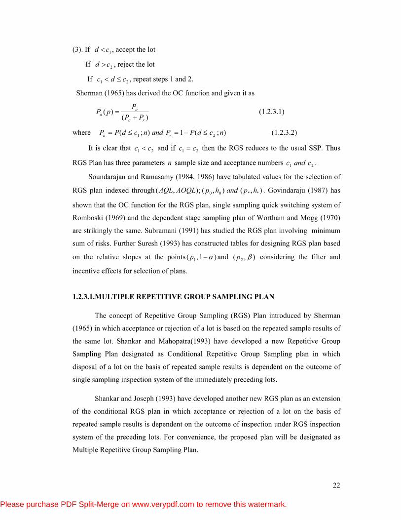
(3). If 1cd < , accept the lot

If 2cd > , reject the lot

If 21 cdc ≤< , repeat steps 1 and 2.

Sherman (1965) has derived the OC function and given it as

)(

)(ra

aa

PP

PpP

+= (1.2.3.1)

where );(1);( 21 ncdPPandncdPP ra ≤−=≤= (1.2.3.2)

It is clear that 21 cc < and if 21 cc = then the RGS reduces to the usual SSP. Thus

RGS Plan has three parameters n sample size and acceptance numbers 21 candc .

Soundarajan and Ramasamy (1984, 1986) have tabulated values for the selection of

RGS plan indexed through ),(),();,( **00 hpandhpAOQLAQL . Govindaraju (1987) has

shown that the OC function for the RGS plan, single sampling quick switching system of

Romboski (1969) and the dependent stage sampling plan of Wortham and Mogg (1970)

are strikingly the same. Subramani (1991) has studied the RGS plan involving minimum

sum of risks. Further Suresh (1993) has constructed tables for designing RGS plan based

on the relative slopes at the points )1,( 1 α−p and ),( 2 βp considering the filter and

incentive effects for selection of plans.

1.2.3.1.MULTIPLE REPETITIVE GROUP SAMPLING PLAN

The concept of Repetitive Group Sampling (RGS) Plan introduced by Sherman

(1965) in which acceptance or rejection of a lot is based on the repeated sample results of

the same lot. Shankar and Mahopatra(1993) have developed a new Repetitive Group

Sampling Plan designated as Conditional Repetitive Group Sampling plan in which

disposal of a lot on the basis of repeated sample results is dependent on the outcome of

single sampling inspection system of the immediately preceding lots.

Shankar and Joseph (1993) have developed another new RGS plan as an extension

of the conditional RGS plan in which acceptance or rejection of a lot on the basis of

repeated sample results is dependent on the outcome of inspection under RGS inspection

system of the preceding lots. For convenience, the proposed plan will be designated as

Multiple Repetitive Group Sampling Plan.


23

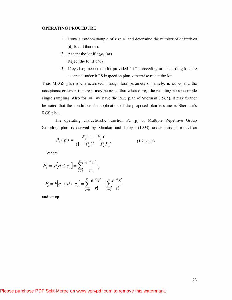
OPERATING PROCEDURE

1. Draw a random sample of size n and determine the number of defectives

(d) found there in.

2. Accept the lot if d≤c1 (or)

Reject the lot if d>c2

3. If c1<d<c2, accept the lot provided “ i “ proceeding or succeeding lots are

accepted under RGS inspection plan, otherwise reject the lot

Thus MRGS plan is characterized through four parameters, namely, n, c1, c2 and the

acceptance criterion i. Here it may be noted that when c1=c2, the resulting plan is simple

single sampling. Also for i=0, we have the RGS plan of Sherman (1965). It may further

be noted that the conditions for application of the proposed plan is same as Sherman’s

RGS plan.

The operating characteristic function Pa (p) of Multiple Repetitive Group

Sampling plan is derived by Shankar and Joseph (1993) under Poisson model as

i

ac

i

c

i

caa

PPP

PPpP

−−

−=

)1(

)1()( (1.2.3.1.1)

Where

[ ] ∑=

−

=≤=1

0

1!

c

r

rx

ar

xecdPP ,

[ ] ∑∑=

−

=

−

−=<<=12

00

21!!

c

r

rxc

r

rx

cr

xe

r

xecdcPP

and x= np.


24

SECTION 1.3:

This Section includes a brief description of Suspension System and review on

Two Plan System.

1.3.1. REVIEW ON ONE PLAN SUSPENSION SYSTEM

This section gives a brief review on suspension system proposed by Troxell (1972).

Cone and Dodge (1962) have first shown that the effectiveness of a small sample

lot-by-lot sampling system can be greatly improved by using cumulative results as a basis

for suspending inspection. Suspending inspection requires the producer to correct what is

wrong and submit satisfactory written evidence of action taken before inspection is

resumed. The small sample is due to small quantity of production or costly or destructive

nature of sample. Usually small sample size is not very effective since the discrimination

between good and bad quality is not sufficient. Hence Cone and Dodge(1962) used the

cumulative results principle to suspend inspection.

Troxell (1972) has applied this suspension principle to acceptance

sampling system incorporating a suspension rule to suspend inspection on the basis of

unfavourable lot history, when small sampling plans are necessary or desirable. Here

suspension rule is seen to be a stopping time random variable and a suspension system is

a rule used with a single sampling plan or a pair of normal and tightened sampling plans.

When single plan is used with a suspension rule it is called One Plan (OP) suspension

system. Similarly when two plans, tightened and normal are used it is called Two plan

(TP) suspension system.

General Description about Suspension System

A suspension rule, which is designated as (j, k), 2 ≤ j ≤ k, is a rule for suspending

inspection based on finding j lot rejections in k or less lots. Specifically, an account is

kept of lot dispositions from the present lot to a fixed number of (k-1) previous

consecutive lots. If at any time the present lot increases the total number of lot rejections

observed over the fixed span of length k to some predetermined integer j, inspection is

suspended; a run of j out of k or less lots is said to have occurred. Given j and k, at least j

lots must be inspected before a decision is possible upon the beginning of a new process

or from the time of the last suspension. Upon restart of inspection after suspension,

history starts a new in that all previous dispositions are ignored. The rule then determines

uniquely at every lot whether to continue or suspend inspection.


25

The phrase “lot disposition” always refers to either lot acceptance (a) or lot

rejection (R), while the term ‘lot history’ refers to a sequence of lot dispositions

e.g.(AARARA….). A one plan suspension system is a combination of a suspension rule

and a single lot-by-lot sampling plans. In an OP suspension system, a lot-by-lot sampling

plan is used in the usual way to decide whether individual lots shall be accepted or

rejected. The sampling inspection procedures being treated here is one involving the

sampling of a continuous process with samples taken from each lot or partition of the

product. The conditions for application are given below:

Conditions for Applications:

1. Production is steady, so that the results on current and preceding lots are

broadly indicative of a continuous process.

2. Samples are taken from lots substantially I the order of production so that

observed variation in quality of product reflect process performance.

3. Inspection is performed close to the production source so the inspection

information can be made available promptly.

4. Inspection is by attributes, with quality measured in terms of fraction

defective p.

5. A single sample of size, n or double or multiple samples of equal size n is

taken from each sampled lot.

Operating Procedure

1. For the product under consideration establish a reference quality level

(RQL). This RQL termed as np represents the desired quality at delivery

considering the needs of service and cost of production.

2. Consider the established RQL, select a suspension system.

3. Apply the suspension rule to the first, second…kth lot, then to each

successive group of k lots.

4. If any lot is rejected, declare the lot nonconforming and dispose it in

accordance with standard procedures.

5. If for any lot, the suspension rule occurs, declare the current lot

nonconforming and also declare the process nonconforming.

6. When the process is judged nonconforming:


26

a. Notify the submitting agency that no additional lots may be

submitted for inspection until that agency has furnished evidence,

satisfactory to the inspection agency that action has been taken to

assure the submission of satisfactory material.

b. Dispose the current nonconforming lot in accordance with standard

procedures.

c. When satisfactory evidence of corrective action is furnished, start

inspection again with the next succeeding lot and with this lot

begin accumulation.

d. If it becomes necessary to refuse lot submissions a second time, so

advice an appropriate higher authority and notify the submitting

agency that further submissions will be refused until evidence

satisfactory to the higher authority has been approved

Average Run Length

According to Troxell (1972) the expected time to suspension or average run length

of a rule is important in the evaluation of the suspension system. The average run length

of the suspension rule (j, k) designated as ARL (j, k) can be calculated in the following

way.

First, the expected number of lot rejections until suspension is calculated. Since

lot rejections are interspaced with lot acceptances, the second step is to find the total

expected number of lots inspected, including the rejected lot, between successive lot

rejections, the ARL equals the sum of the total number of lots inspected until suspension.

It is shown that, in fact the total number of inspected lots between consecutive rejections

are independently and identically distributed for all rejections so that:

ARL (j, k) = (Total number of inspected lots between two

rejections) × (expected number of rejection until

suspension).

Using this fact, for j=2, the expression is given by a single term and for j=3, the

result is best expressed in the form of a continued fraction, which is found by solving for

the stationary distribution of a particular Markov chain. For higher rules, a discussion is

given indicating the method of solving for the expected number of rejections until

suspension.


27

Troxell (1972) has derived the following results:

i) ARL for the rule (j, j), j ≥2 is

ARL (j, j) = ( )( ) jaa

j

a

PP

P

−

−−

1

11

ii) ARL for the rule (j, ∞) is

ARL (j, ∞) = aP

j

−1

which is the waiting time for the jth occurrence of a lot rejection, or the mean of the

negative binomial distribution with parameter j.

iii) ARL for the rule (2, k) is

)Pa-Pa)(1-(1

)Pa-(2 k) (2, ARL

1-k

1-k

= , k ≥ 2

For any k such that j < k < ∞ and 0 < Pa< 1

ARL (j, j) > ARL (j, k) > ARL (j, ∞)

So that the rules (j, j) and (j, ∞) respectively are upper and lower bounds for all rules in

the class (j, k).

Operating Characteristic Curve

A different type of OC curve which has features not common to type B OC curve

has been used here to study the suspension system. Since ARL for the rule (j, k) is some

function of incoming quality p, this correspondence allows an operating characteristic to

be plotted in the following way.

In a large number of lots N, the number of lots for which the process is judged

conforming, that is the number of lots for which suspension does not occur, is given

approximately by N(1-1/ARL). Therefore 1-1/ARL is interpreted as the average fraction

of lots for which the process is acceptable, or the probability of accepting the process.

This value is denoted as PA,

PA (j, k) =1-1/ARL (j, k) and hence

12

1),2(

−−

−+=

k

a

k

aa

AP

PPkP (1.3.1.1)


28

2

1),2(

a

A

PP

+=∞ (1.3.1.2)

The OC Curve is a graph of PA as a function of fraction defective.

Operating Ratio

A usual measure of discrimination of a sampling plan is the operating ratio (OR),

defined as the ratio of the two values of fraction defective for which the probability of

acceptance of lots is 0.10 and 0.95 respectively or OR= p0.10/p0.95. In order to assess the

ability of the rules in anyone class to discriminate between good and bad quality, an index

called the Operating Ratio is often used. The operating ratio was first proposed by Peach

(1947) for measuring quantitatively the relative discrimination power of sampling plans.

The operating ratio for a suspension system is defined as follows:

Choose α and β, where for the particular class (j, k), α and β are restricted such

that 1-1/j ≤ β < α ≤ 1. α and β are probabilities of not suspending inspection (PA)

corresponding to ARL’s of 1/1- α and 1/1-β, hence the restriction. It is necessary to find

the fractions defective pα and pβ which yield α and β, for any rule (j, k) and sampling plan

(n, c). The OR is defined as the ratio of the two fractions defective for which the

probability of not suspending is β and α, that is OR = pβ/ pα.

It is desired to refer a suspension system by a numerical value of the OR, a

subjective choice of α and β is made. The choice of α is 0.98, corresponding to an ARL

of 50. The fraction defective value, which gives this answer, is denoted as p0.98 . That is,

OR = p0.80/ p0.98. For different values of α and β that is for different values of ARL it is

possible to define and calculate OR. But two values of ARL, 50 and 5 are proposed as

standards which are used to define the OR of a sampling plan.

Designing of suspension system:

Troxell (1972) has designed a suspension system for a particular production

process and construction are used through reference quality level. A second reference

quality level which represents an undesirable value of quality is also used. These two

reference quality levels are referred respectively as, RQL1 and RQL2 with RQL1 < RQL2

and represent standards of quality, taking in to consideration production demands,

specifications and costs.

Associated with RQL1 a value of ARL is chosen such that the statement (1) may

be agreed upon by producer and consumer.


29

1. If quality is at RQL1 or better, then on the average at least ARL1 lots should be

inspected before suspension occurs.

If the quality is at RQL2 a statement of the form (2) may be used.

2. If the quality is at RQL2 or poorer, then on the average at the most ARL2 lots

should be inspected before suspension occurs.

Troxell (1972) has used ARL to determine a measure of the risk involved in using

a suspension system similar to the producers and consumer’s risk of sampling schemes.

At RQL1, the producer’s risk of having inspection suspended when quality is at an

acceptable level is at the most once in ARL1 lots. At RQL2, the consumers risk in

continuing inspection when quality is at a rejectable level is that, at most ARL2 lots on the

average should be inspected from suspension to suspension.

Designing a suspension system involves first selecting those rules which satisfy

statement (1) or simultaneously (1) and (2) and then using a criterion to choose a single

system from these rules. In selecting the set of rules, not that any fraction defective p,

ARL (j, j) > ARL (j, j+1) > ARL (j, j+2)>…………….> ARL (j, ∞)

According to Troxell (1972) for choosing a suspension system two criteria are

available. The first criterion is discrimination power based on the conjecture that the

rules in a class are ordered from (j, j) to (j, ∞) according to their power to discriminate

from best to worst. The other criterion uses the fact that for any fixed ARL, the

associated value of fraction defective monotonically decreases from the rule (j, j) to the

rule (j, ∞).

When the sample size is not specified it can be found out from the formula n= log

Pa/Log (1-p). Let n (k) be the sample size for the rule (2, k). From the result n(2) ≥ n(3)

≥ ………………≥ n(∞), it can be seen that the rule (2,2) has the best discrimination but

uses the largest sample size among all (2, k) rules.

Designing of suspension system and its Procedures

Troxell (1972) has outlined four procedures for choosing a suspension system,

two with the sample size chosen by the user and two with the sample size chosen from

tables. In all cases the user must decide on a value for RQL1 and has option to use or not

to use RQL2.


30

A. RQL1 and n specified

1. Select the desired values of RQL1 and n.

2. Choose ARL1 from one of the reference values in tables.

3. Use tables to find the rules (2,2), …….,(2,last) which have fraction

defective p ≥ RQL1

4. (a) Use (2, 2) for best discrimination

(b) Use (2, last) for the rule having actual fraction defective closest to

RQL1.

5. If no (2, k) rule exists use the class (3, k) and follow step 1 through 4.

If no (2, k) rules exist for the desired values of n and RQL1, generally the class (3, k) will

furnish at least one. Nevertheless the class (2, k) has rules having minimum ARL when

quality is hundred percent defective. Requirements should be reviewed to see if RQL1

may be decrease to just equal to the fraction defective value for (2, 2) in which case a rule

having good sample size could be increased until the rule (2, 2) just qualifies.

B. RQL1, RQL2 and n specified

1. Select the desired values of RQL1, RQL2 and n.

2. Choose ARL1 and ARL2.

3. Use tables to find the rules (2, first)… (2, last) which have p≥RQL1, at

ARL1 and p≤ RQL2 at ARL2.

4. (a) Use (2, first) for best discrimination

5. (b) Use (2, last) for closeness at RQL1.

6. If no (2, k) rule exists use the class (3, k) and follow step 1 to 4.

If no (2, k) rule exists, the two RQL values are two restrictive in the sense that

RQL2/ RQL1 is too long; the sampling plan procedure in this case is to increase the

acceptance number, c. In the case when no rule exists satisfying both statements (1)

and (2), it is Troxell’s belief that the conditions are two restrictive for c=0 suspension

system and that a sampling plan which c ≥ 1 is called for, it can be chosen to suit the

situation.

C. RQL1 specified

1. Select the desired values of RQL1.

2. Choose ARL1 from one of the reference values in tables.


31

3. Use the tables for each rule to find the smallest value of n such that p ≥ RQL1

4. a). Use (2, 2) for best discrimination

b). Use (2, 10) for the rule having smallest sample size.

Troxell (1980) prefers to use the rule (2, 2) despite the larger sample size, because

of its discrimination power and the simplicity of the rule itself. Also steps 1 through 4

may be used for all the rules in the class (3, k) listed in tables.

D. RQL1 and RQL2 specified

1. Select the desired values of RQL1 and RQL2.

2. Choose ARL1 and ARL2.

3. Use table for each rule to find two integers n1 and n2 such that p ≥ RQL1

for n1 and p ≤ RQL2 for n2.

4. a). Use n1 to match the suspension system, as closely as possible to RQL1.

b). Use n2 to match the suspension system, as closely as possible to RQL2.

In order those statements (1) and (2) to be satisfied, the sample size must be at most n1

and at least n2. However when the ratio RQL2 / RQL1 is very low, it may turn out that n1 <

n2 in which case no solution exists. If n2 < n1 then any integer from n2 to n1 may be used.

When no solution exists, the conditions to use a c = 0 suspension system are too severe.

Troxell (1980) has given one example to explain the procedure B.

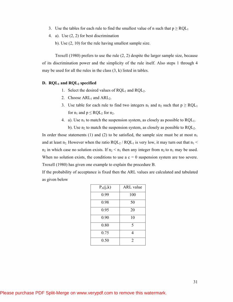
If the probability of acceptance is fixed then the ARL values are calculated and tabulated

as given below

PA(j,k) ARL value

0.99 100

0.98 50

0.95 20

0.90 10

0.80 5

0.75 4

0.50 2


32

1.3.2. REVIEW ON GENERALIZED TWO-PLAN SYSTEM

Dodge (1959) proposed a new sampling inspection system namely two-plan

system. The two-plan system has a normal as well as a tightened plan which has a tighter

OC curve compared with that of the normal plan. The system is largely incorporated in

the MIL-STD-105E (1989) for designing of a sampling system. The switching rules of a

Generalized Two-Plan System are

Normal to Tightened

When normal inspection is in effect, tightened shall be instituted when‘s’ out of

‘m’ consecutive lots or batches have been rejected on original inspection(s<m).

Tightened to Normal

When tightened inspection is in effect, normal shall be instituted when‘d’

consecutive lots or batches have been considered acceptable on original inspection.

Kuralmani (1992) has shown that the composite OC and ASN functions using the

above measures,

Pa (p) = IN PN + IT PT

ASN (p) =IN nN + IT nT

Where nN = the (average) sample size of normal inspection plan.

nT = the (average) sample size of the tightened inspection plan.

Markov chain approach is used for designing the various measures of performance

measures of the Generalized Two-Plan System.

The events and definitions are given below:

Ni = the event that the normal inspection is in effect (i = 1,2,…m)

Ti = the event that the tightened inspection is in effect (i = 1,2,…d)

PNi = the probability of the system being in state Ni ( i = 1,2,…m)

PTi = the probability of the system being in state Ti (i = 1,2,…d)

For the sake of the convenience, let us denote PN and PT as ‘a’ and ‘b’ respectively

for evaluating the above measures.

All probabilities can now be evaluated using the condition that the sum of all

probabilities equals to one, i.e,

IN + IT = 1

One can get, IN = τµ

µ+

and IT = τµ

τ+


33

Where, 12

22

)1)(1(

)12()1(1−+−

+−−

−−

−−−+=

ssm

sms

aaa

aaaµ

= the average number of lots inspected using the normal

plan before going to tightened inspection.

d

d

bb

b

)1(

1

−

−=τ

= the average number of lots inspected using the normal

plan before going to tightened inspection.

Here, a as PN and b as PT, the composite OC and ASN functions are, respectively,

obtained as Pa (p) = τµτµ

+

+ TN PP (1.3.2.1)

Where PN = Probability of acceptance under the normal inspection.

PT = Probability of acceptance under the tightened inspection

Note that where µ and τ are the average number of lots inspected using normal

inspection before going to tightened inspection and average number of lots inspected

using tightened inspection before going to normal inspection respectively.

Thus the Generalized Two-Plan system can be used to design a desired sampling

system viz. QSS – d and Two-Plan (2 out of m) systems of Romboski (1969), TNT

scheme of Calvin (1977). For example, for (s = m = 1), then the Generalized Two-Plan

System becomes QSS – d system. Similarly the other systems can be deduced from the

Generalized Two-Plan is very useful to find performance measures of a desired sampling

system by substituting numbers for s, m, and d.

Two Types of Two-Plan System (TPS)

1. A single sampling two-plan system (TPS) with equal sample size but with

different acceptance numbers.

2. A single sampling two-plan system (TPS) with two different sample sizes but

with same acceptance number.

Let us designate the first and second types of TPS as TPS-(n; cN ,cT) and

TPS-(n,kn;c) respectively. The expressions for PN, PT of TPS-(n; cN, cT) system

are given by PN = P(d ≤ cN / n, p)

PT = P(d ≤ cT / n, p)

For TPS-(n, kn; c) system one has

PN = P (d≤ c / n, p)

PT = P (d ≤ c/ kn, p)


34

SECTION 1.4:

This section contains A brief survey on Chain Sampling Plan , Three Stage Chain

Sampling plan and Skip-lot Sampling Plan.

1.4.1. CHAIN SAMPLING PLAN

A review on Chain Sampling Plan (ChSP-1) and Chain Sampling Plan(0,1) is given

in this section.

Sampling inspection in which the criteria for acceptance and non- acceptance of a

lot depends on the results of the inspection of immediately preceding lots is adopted in

Chain Sampling Plans which was proposed by Dodge (1955).

For situations involving costly or destructive testing by attributes, it is the usual

practice to use single sampling plan with smaller sample size and acceptance number zero

to have the decision either to accept or reject the lot. The small sample size is warrented

with cost of the test and the zero acceptance number arising out of the desire to maintain a

steeper OC curve. The single sampling plan is the basic one to all acceptance sampling

plans. The major advantage of the attribute single sampling plan is the simplicity to use

among all types of acceptance sampling plans. But, the single sampling plan with

acceptance number zero has the following undesirable characteristics namely,

i) A single occasional non conforming unit in the sample calls for the rejection of

the lot and

ii) The OC curves of all such sampling plans have a uniquely poorer shape, in that

the probability of acceptance starts to drop rapidly for smaller values of the

percent non- conforming unit.

Chain Sampling Plan (ChSP-1) proposed by Dodge (1955), making use of

cumulative results of several samples help to overcome the short comings of the single

sampling plan when c=0.

CONDITIONS FOR APPLICATION OF ChSP-1:

1. The cost of destructiveness of testing is such that a relatively small sample size is

necessary, although other factors make a larger sample desirable.

2. The product to be inspected comprises a series of successive lots produced by a

continuing process.

3. Normally lots are expected to be essentially of the same quality.

4. The consumer has faith in the integrity of the producer.


35

Operating Procedure:

The plan is implemented in the following way:

1. For each lot, select a sample of size n units and test each unit for conformance to

the specified requirements.

2. Accept the lot if d (the observed; number defectives) is zero in the sample of n

units, and reject it if 1>d

3. Accept the lot if d is equal to 1 and if no defectives are found in the immediately

preceding i samples of size n .

Dodge (1955a) has given the operating characteristic function for ChSP-1 as

[ ]ia nPnPnPpP );0();1();0()( += (1.4.1.1)

where

=);( ndP Probability of getting exactly d nonconforming units in a sample of sizen for

given product quality p having .10 ord =

The Chain Sampling Plan (ChSP-1) is characterized with parameters n and i .

When ,∞=i the OC function of a ChSP-1 plan reduces to the OC function of the single

sampling plan with acceptance number zero and when ,0=i the OC function of ChSP-1

plan reduces to the OC function of the single sampling plan with acceptance number c=1.

The use of cumulative results of several samples are proposed for application to

cases where there is repetitive production under the same conditions and where the lots or

batches of product to be inspected are submitted for acceptance in the order of

production. Such situations may arise in receiving inspections of continuing supply of

purchased materials produced within a manufacturing plant. The plan is not suited to

intermittent or job- lot production or occasional purchases.

When large samples are practicable, the use of a 0=c plan is warranted. A double

sampling plan avoids the above shortcomings of single sampling 0=c plans , but chain

sampling has a consistent inspection than double sampling for a given degree of

discrimination.


36

Clark (1960) has provided OC curves for different combinations o f n and i and

also compares ChSP-1 plans with single sampling plan. Soundararajan (1978 a,b)

constructed tables for the selection of ChSP-1 plans under Poisson model and also gives

formula for i which minimizes the sum of producer’s and consumer’s risk with

specified LQLandAQL , when sample size is fixed. Schilling (1982) and Stephens

(1982) have provided a detailed discussion on ChSP-1 plan. Soundararajan and

Govindarajan (1982) have also studied ChSP-1 involving minimum sum of producer’s

and consumer’s risk. Soundararajan and Doraisamy (1984) have studied the ChSP-1 plan

indexed through .MAPDandIQL Govindaraju (1990b) tabulated values for the selection

of ChSP-1 plan using search procedure. Subramani (1991) has studied the ChSP-1 plan

involving minimum sum of risks. Further Suresh (1993) has constructed tables for

designing ChSP-1 plan based on the relative slopes at the points )1,( 1 α−p and ),( 2 βp

considering the filter and incentive effects for selection of plans.

A generalized family of two- stage chain sampling plans, which are extension of

ChSP-1 plans, we proposed by Dodge and Stephens (1966). The sampling procedure

involves the use of cumulative results from the current sample and one or more previous

sample for making the decision regarding the acceptance or rejection of the current lot.

The procedure make use of the stages, each of which stipulates the sample size, the

number of samples over which the cumulative results are taken, and the allowable number

of nonconforming units applicable to that stage.

The OC function of ChSP-(0,1) plan derived by Dodge and Stephens (1966) is

Pa (p) = ,]);0(1[);0();1();0(1

]);0(1[);0();1()];0(1)[;0(1121

121

−−

−

−+−

−+−kkk

kkk

nPnPnpnP

nPnpnPnPnP k2>k1 (1.4.1.2)

Where,

P (0;n) = Probability of getting exactly zero nonconformities in a sample of Size n and

P(0;1) = Probability of getting exactly one nonconforming unit in a sample of size n.

Here, it can noted that, the Chsp-1 plan and the Chsp-(0, 1) plan will become

identical whenever i=k1 = k2-1. Like Chsp-1 plan, the disadvantages of the single

sampling plan having Ac=0 mentioned earlier, are also overcome in Chsp-(0,1) plan.


37

1.4.2. THREE STAGE CHAIN SAMPLING PLAN

This section deals with the review on three stage chain sampling plan of type

ChSP (0, 1, 2) introduced by Soundararajan and Raju (1984), extending the concepts used

by Dodge (1955) and Dodge and Stephens (1966).

For situations involving costly or destructive testing by attributes, it is the usual

practice to use single sampling plan with a small sample size and an acceptance number

zero to base the decision to accept or reject the lot. The sample size is dictated by the cost

of the test and the zero acceptance number arises out of desire to maintain a steeper OC

curve. Single sampling plan with acceptance number has zero has the following

undesirable characteristics.

1. A single defect in the sample calls for rejection of the lots (or for

classifying the lot as non-conforming), and

2. The OC curves of all such sampling plans have a uniquely poorer shape, in

that the probability of acceptance starts to drop rapidly for the smallest

values of percent defective.

Dodge (1955) treats this problem by a procedure, called chain sampling plan

(ChSP – 1). These plans make use of the cumulative inspection results form several

results, from one or more samples along with the results from the current sample, in

making a decision regarding acceptance or rejection of the current lot. The chain

sampling plans are applicable for both small and large samples. They have been found

particularly advantageous in circumstances where samples are small, as when tests are

destructive and costly.

Fred Frishman (1960) has proposed two approaches to the use of other acceptance

numbers different from 0 and 1 of ChSP – 1, that employ modified procedural rules

including conditional cumulation and a provision for rejecting a lot on the basis of the

results of a single sample. Dodge and Stephens (1966) extended the concept of chain

sampling plans and presented a set of two-stage chain sampling plans based on the

concept of ChSP – 1 developed by Dodge (1955). They presented expressions for OC

curves of certain two – stage chin sampling plans and made comparison with single and

double sampling attributes inspection plans.


38

The three stage chain sampling plan of type ChSP (0, 1, 2) developed by

Soundararajan and Raju (1984) is a generalization of Dodge (1955) chain sampling plan

ChSP – 1 and Dodge and Stephens (1966) chain sampling plan ChSP – (0, 1).

Soundararajan and Raju (1984) gives the structure and operating procedure of generalized

three – stage chain sampling plan and expressions for OC curve of certain three – stage

plans are also given.

ChSP (0, 1, 2) can be used for both small and large samples, but it is particularly

useful when samples must necessarily be small (eg., when tests are costlier). The greater

generality in the choice of parameters in the ChSP – (0, 1,2) plan allows for greater

flexibility in matching these plans to other plans, and allows for improved discrimination

between good and bad quality. A more complete discussion on chain sampling plan can

be found in Schilling (1982).

General Plan

The general plan involves the use of cumulative results from the current sample

and one or more previous samples in making the decision regarding the acceptance or

rejection of the current lot. The procedure makes use of three-stages, each of which

stipulates the sample size, the number over which the cumulative results are taken, and

the allowable number of defectives applicable to that stage. The overall procedure

involves a restart of the cumulative results. i.e., a return to the criterion of the first stage,

following a cumulative type rejection at any stage. The general plan has two basic

procedures.

A. Normal Procedure:

Normally used by the inspector when quality is good, as evidenced by acceptance

of a number of successive lots. For this procedure the inspector uses cumulative results

for a fixed number of samples, the current sample plus some stated number of preceding

samples, and accepts the current lot if the cumulative results meet the cumulative results

criterion (CRC).

B. Restart Procedure:

This used at the start of application, and for lots immediately following a lot that

has been rejected, and until a sufficient number of lots are accepted to permit using a


39

normal procedure. During this interim or restart period, sample results are cumulated

starting with the first lot following the rejected lot, and lots are accepted if they meet the

particular cumulative results criterion or criteria that have been established for the restart

period.

In operation the general plan will involve a continuing of acceptances by the

normal procedure, the “steady state” broken by transient period of restart operations

wherever individual lots are rejected. The overall characteristics of the plan are markedly

influenced by the choice of parameters for the overall procedure, Viz. the sample size, the

maximum number of samples to be used in cumulations, the cumulative acceptance

criterion used for the normal procedure, and the number and the character of the

cumulative acceptance criteria used in the restart period.

The generalized three – stage chain sampling plan, called “three – stage” because

its restart period has three stages, with three corresponding acceptance criteria. As shown,

the acceptance criterion used in the third stage of the restart period is the same as that

used in the normal procedure.

Operating Procedure

Step 1: At the outset, select a random sample of n units from the lot and from each

succeeding lot.

Step 2: Record the number of defectives d, in each sample and sum the number of

defectives, D, in all samples from the first upto and including in the current

sample.

Step 3: Accept the lot associated with each new sample during the cumulation as

long as Di < c1; 1< i < k1.

Step 4: When k1 consecutive samples have all resulted in acceptance continue to

sum the defectives in the k1 samples plus additional samples upto not more

than k2 samples.


long as Di < c2; k1 < i < k2.

Step 6: When k2 consecutive samples have all resulted in acceptance continue to

sum the defectives in the k2 samples plus additional samples upto not

more than k3 samples.


long as Di < c3; k2 < i < k3.


40

Step 8: When the third stage of the restart period has been successfully completed

(i.e., k3 consecutive samples have been resulted in acceptance), start

cumulation of defectives as a moving total over k3 samples by adding the

current sample result while dropping from the sum, the sample result of

the k3th preceding sample. Continue this procedure as long as Di < c3 and

in each instance accept the lot.

Step 9: If for any sample at any stage of the above procedure, Di is greater than the

corresponding c, reject the lot.

Step 10: When a lot is rejected return to Step-1 and a fresh restart of the

cumulation procedure.

When k1=1, k2=2 and k3=3 and c2=c1+1, c3=c2+1, the three stage chain sampling plan

becomes a multiple sampling plan. Thus three-stage chain sampling plan has better

discriminating power than the multiple sampling plans with equal sample size. In this

thesis we considered the three stage sampling plan of type ChSP (0, 1, 2).

When the sample size is not more than one-tenth of the lot size, and when the

quality is measured interms of defectives, the OC curve can be computed using the

binomial model. In addition to the condition of sample size being not more than one-tenth

of the lot size, if the lot quality p (measured interms of defectives) is less than or equal to

0.01, the OC curve can be based on the Poisson model. When the quality is measured in

terms of defects, the appropriate model is also the Poisson one.

Under the condition for application of the Poisson model the probability of

accepting a lot given the proportion non-conforming under the ChSP-(0,1,2) plan with

parameters n, k1, k2, k3, c1, c2, and c3 was derived by Raju (1984) as

( )

( ) ( )( )

( )

( ) ( )( )

−

−+

−

−+

−

−−−

+−+

−

−+

−

−+

−

−+

−

−−−

+−+

−

−++−−++

=

−−−−−−

−−−

−−−−−−

−−−

−−−

0

1

0

022

0

2

00

0

2

023

0

2

1

1

0

2

112

0

1

0

01

0

1

0

022

0

2

00

0

2

023

0

2

1

1

0

2

112

0

1

0

01

1

02

2

0

2

123

1

010

1

1

1

1

1

11

1

11

1

1

1

1

1

11

1

1)1(

)(

23

2

2323

2

2

12

1

23

2

2323

2

2

12

1332

P

PPP

P

PP

P

PkkPP

PPkkP

PPP

P

PPP

P

PP

P

PkkPP

PPkkP

PPPPPPPkkPPP

pP

kk

k

kkkk

k

k

kk

k

kk

k

kkkk

k

k

kk

kkkk

a

(1.4.2.1)


41

Where,

P0= Probability of getting exactly zero non- conforming in a sample of size n

P1= Probability of getting exactly one non- conforming in a sample of size n

P2= Probability of getting exactly two non- conforming in a sample of size n

It is well known that for a series of lots from a process, the binomial model for the

OC curve will be exact in the case of fraction non-conforming. It can be satisfactorily

approximated with the Poisson model where p is small, n is large, and np < 5 when the

quality is measured in terms of non conformities, the Poisson model is the appropriate

one.

Under the Poisson assumption, the expression for

P0= e-np, P1= np e

-np, P2= ((np)

2/2) e

-np

1.4.3. REVIEW ON SKIP-LOT SAMPLING PLAN

Skip –lot Sampling Plans are a system of lot by lot inspection plans in which a

provision is made for inspection only some fraction of the submitted lots. Generally Skip

– Lot Sampling Plans should be used only when the quality of the submitted product is

good as demonstrated any inspection or text programme which normally calls for periodic

checking of a continuing out put. This general plan suggested by Dodge (1955) is

designated as SkSP -1. He initially presented Skip – lot Sampling plans as an extension

of Continuous Sampling plan.

A Skip – lot sampling plan is the application of continuous sampling to lots rather

than to individual units. SkSP-1, due to Dodge, results in the lot acceptability or non-

acceptability and applied to the chemical and physical analysis with a basis for reducing

the costs of testing under the following conditions:-

• The product comprises a series of successive purchased raw

materials from the same source having the same quality.

• The specified requirements are expressed as maximum or minimum limits

for one or more chemical characteristics.


42

• For a given characteristic, the normal acceptance procedure for each lot is

to obtain a suitable sample of the material and make a lab analysis of test of it.

Operating Procedure of SkSP -1

1. The Sksp -1 plan is to be applied separately to each of the characteristics

under consideration.

2. For given characteristic one of the two following procedures A1, or A2 is

chosen.

3. Procedure A1:-

This procedure is applicable when each non-conforming lot is to be either

corrected or replaced by a conforming one. Various steps of this procedure are outlined

below:-

I. At the outset, test each lot consecutively as purchased and continue

such testing until 14 lots in succession are found to be conforming.

II. When 14 lots in succession are found to be conforming, discontinue

testing every lot and instead test only half of the lot.

III. If a tested lot is found to be non-conforming, revert immediately to

testing every succeeding lot until again 14 lots in succession are

found conforming.

IV. Accept the non-conforming lot, if any, either by correcting it or by

replace it by a conforming one.

4. Procedure A2:-

This procedure is applicable when each non-conforming lot is to be rejected

totally. Various steps of this procedure are listed here:

I), II), III ) as in procedure A1 , replacing 14 by 15 IV ) reject and remove each

non-conforming lot.


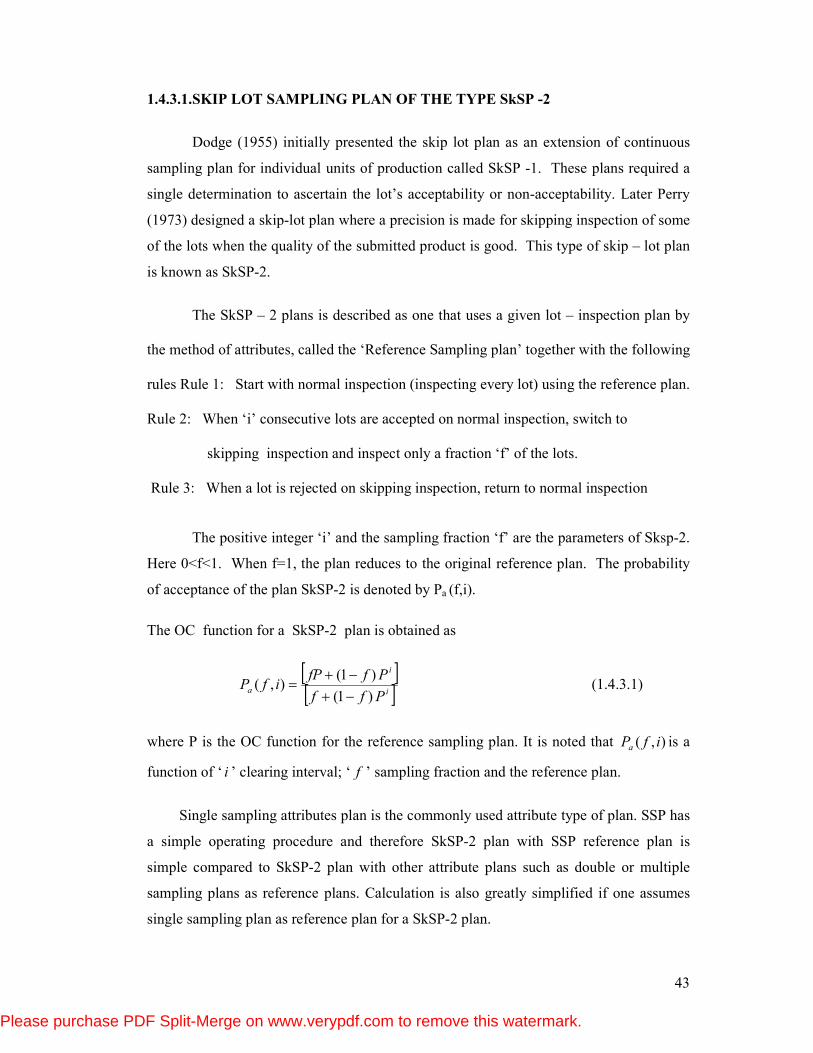
43

1.4.3.1.SKIP LOT SAMPLING PLAN OF THE TYPE SkSP -2

Dodge (1955) initially presented the skip lot plan as an extension of continuous

sampling plan for individual units of production called SkSP -1. These plans required a

single determination to ascertain the lot’s acceptability or non-acceptability. Later Perry

(1973) designed a skip-lot plan where a precision is made for skipping inspection of some

of the lots when the quality of the submitted product is good. This type of skip – lot plan

is known as SkSP-2.

The SkSP – 2 plans is described as one that uses a given lot – inspection plan by

the method of attributes, called the ‘Reference Sampling plan’ together with the following

rules Rule 1: Start with normal inspection (inspecting every lot) using the reference plan.

Rule 2: When ‘i’ consecutive lots are accepted on normal inspection, switch to

skipping inspection and inspect only a fraction ‘f’ of the lots.

Rule 3: When a lot is rejected on skipping inspection, return to normal inspection

The positive integer ‘i’ and the sampling fraction ‘f’ are the parameters of Sksp-2.

Here 0<f<1. When f=1, the plan reduces to the original reference plan. The probability

of acceptance of the plan SkSP-2 is denoted by Pa (f,i).

The OC function for a SkSP-2 plan is obtained as

[ ][ ]i

i

aPff

PffPifP

)1(

)1(),(

−+

−+= (1.4.3.1)

where P is the OC function for the reference sampling plan. It is noted that ),( ifPa is a

function of ‘ i ’ clearing interval; ‘ f ’ sampling fraction and the reference plan.

Single sampling attributes plan is the commonly used attribute type of plan. SSP has

a simple operating procedure and therefore SkSP-2 plan with SSP reference plan is

simple compared to SkSP-2 plan with other attribute plans such as double or multiple

sampling plans as reference plans. Calculation is also greatly simplified if one assumes

single sampling plan as reference plan for a SkSP-2 plan.


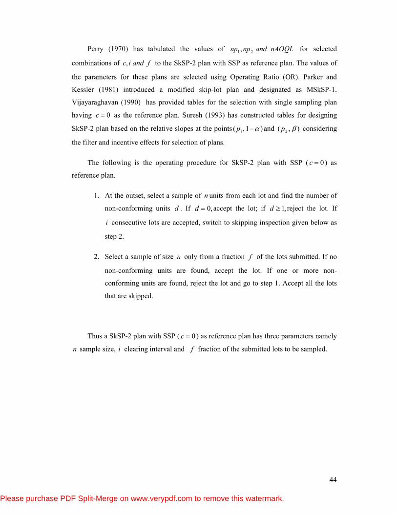
44

Perry (1970) has tabulated the values of nAOQLandnpnp 21 , for selected

combinations of fandic, to the SkSP-2 plan with SSP as reference plan. The values of

the parameters for these plans are selected using Operating Ratio (OR). Parker and

Kessler (1981) introduced a modified skip-lot plan and designated as MSkSP-1.

Vijayaraghavan (1990) has provided tables for the selection with single sampling plan

having 0=c as the reference plan. Suresh (1993) has constructed tables for designing

SkSP-2 plan based on the relative slopes at the points )1,( 1 α−p and ),( 2 βp considering

the filter and incentive effects for selection of plans.

The following is the operating procedure for SkSP-2 plan with SSP ( 0=c ) as

reference plan.

1. At the outset, select a sample of n units from each lot and find the number of

non-conforming units d . If ,0=d accept the lot; if ,1≥d reject the lot. If

i consecutive lots are accepted, switch to skipping inspection given below as

step 2.

2. Select a sample of size n only from a fraction f of the lots submitted. If no

non-conforming units are found, accept the lot. If one or more non-

conforming units are found, reject the lot and go to step 1. Accept all the lots

that are skipped.

Thus a SkSP-2 plan with SSP ( 0=c ) as reference plan has three parameters namely

n sample size, i clearing interval and f fraction of the submitted lots to be sampled.


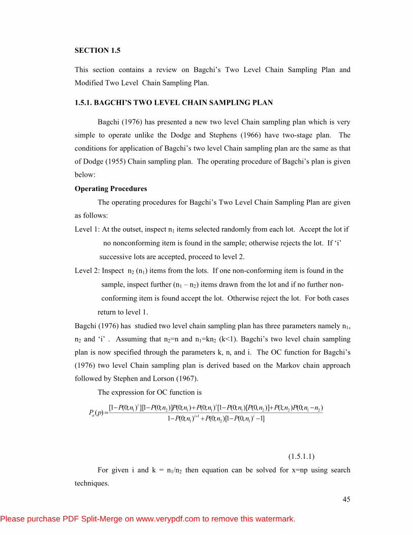
45

SECTION 1.5

This section contains a review on Bagchi’s Two Level Chain Sampling Plan and

Modified Two Level Chain Sampling Plan.

1.5.1. BAGCHI’S TWO LEVEL CHAIN SAMPLING PLAN

Bagchi (1976) has presented a new two level Chain sampling plan which is very

simple to operate unlike the Dodge and Stephens (1966) have two-stage plan. The

conditions for application of Bagchi’s two level Chain sampling plan are the same as that

of Dodge (1955) Chain sampling plan. The operating procedure of Bagchi’s plan is given

below:

Operating Procedures

The operating procedures for Bagchi’s Two Level Chain Sampling Plan are given

as follows:

Level 1: At the outset, inspect n1 items selected randomly from each lot. Accept the lot if

no nonconforming item is found in the sample; otherwise rejects the lot. If ‘i’

successive lots are accepted, proceed to level 2.

Level 2: Inspect n2 (n1) items from the lots. If one non-conforming item is found in the

sample, inspect further (n1 – n2) items drawn from the lot and if no further non-

conforming item is found accept the lot. Otherwise reject the lot. For both cases

return to level 1.

Bagchi (1976) has studied two level chain sampling plan has three parameters namely n1,

n2 and ‘i’ . Assuming that n2=n and n1=kn2 (k<1). Bagchi’s two level chain sampling

plan is now specified through the parameters k, n, and i. The OC function for Bagchi’s

(1976) two level Chain sampling plan is derived based on the Markov chain approach

followed by Stephen and Lorson (1967).

The expression for OC function is

]1),0(1)[;0();0(1

);0();1()],0()[;0(1[);0();0()];0(1][);0(1[)(

12

1

1

212211121

−−+−

−+−+−−=

+ ii

ii

anPnPnP

nnPnPnPnPnPnPnPnPpP

(1.5.1.1)

For given i and k = n1/n2 then equation can be solved for x=np using search

techniques.


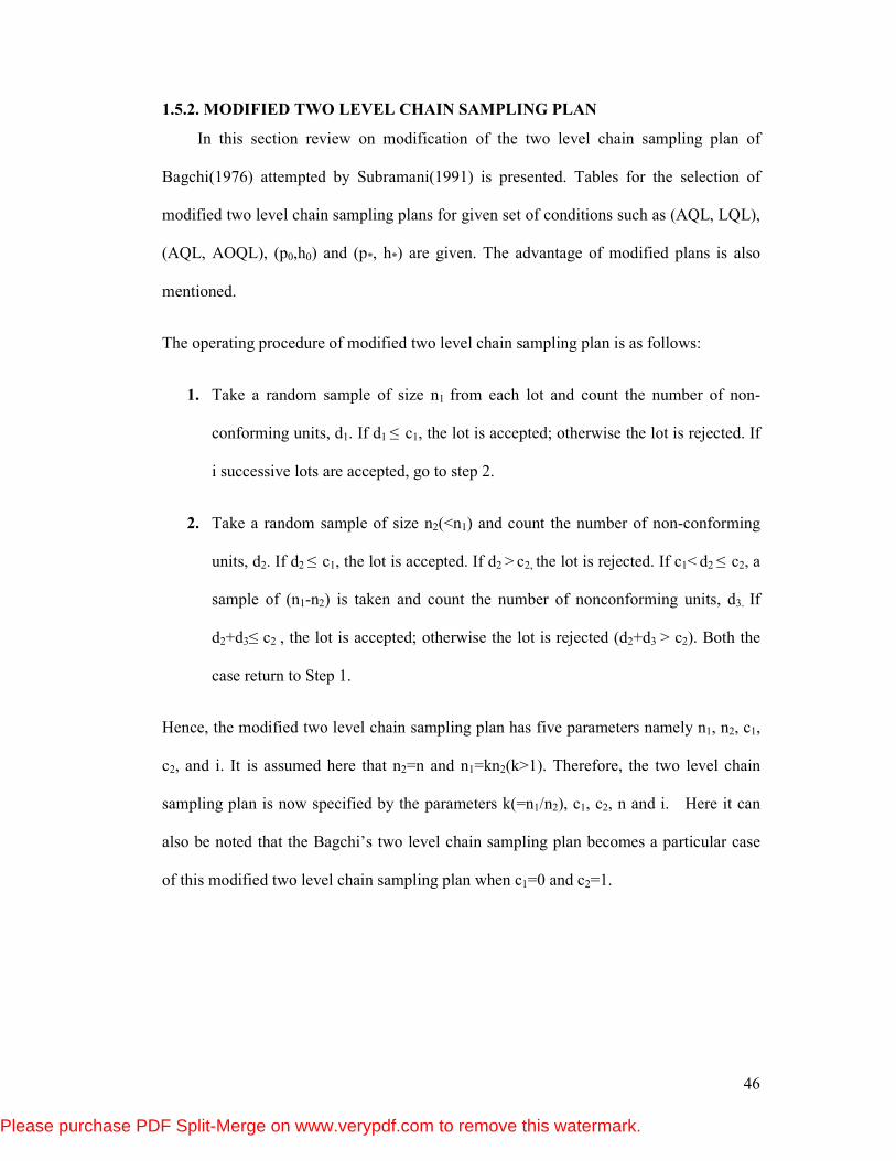
46

1.5.2. MODIFIED TWO LEVEL CHAIN SAMPLING PLAN

In this section review on modification of the two level chain sampling plan of

Bagchi(1976) attempted by Subramani(1991) is presented. Tables for the selection of

modified two level chain sampling plans for given set of conditions such as (AQL, LQL),

(AQL, AOQL), (p0,h0) and (p*, h*) are given. The advantage of modified plans is also

mentioned.

The operating procedure of modified two level chain sampling plan is as follows:

1. Take a random sample of size n1 from each lot and count the number of non-

conforming units, d1. If d1 ≤ c1, the lot is accepted; otherwise the lot is rejected. If

i successive lots are accepted, go to step 2.

2. Take a random sample of size n2(<n1) and count the number of non-conforming

units, d2. If d2 ≤ c1, the lot is accepted. If d2 > c2, the lot is rejected. If c1< d2 ≤ c2, a

sample of (n1-n2) is taken and count the number of nonconforming units, d3. If

d2+d3≤ c2 , the lot is accepted; otherwise the lot is rejected (d2+d3 > c2). Both the

case return to Step 1.

Hence, the modified two level chain sampling plan has five parameters namely n1, n2, c1,

c2, and i. It is assumed here that n2=n and n1=kn2(k>1). Therefore, the two level chain

sampling plan is now specified by the parameters k(=n1/n2), c1, c2, n and i. Here it can

also be noted that the Bagchi’s two level chain sampling plan becomes a particular case

of this modified two level chain sampling plan when c1=0 and c2=1.


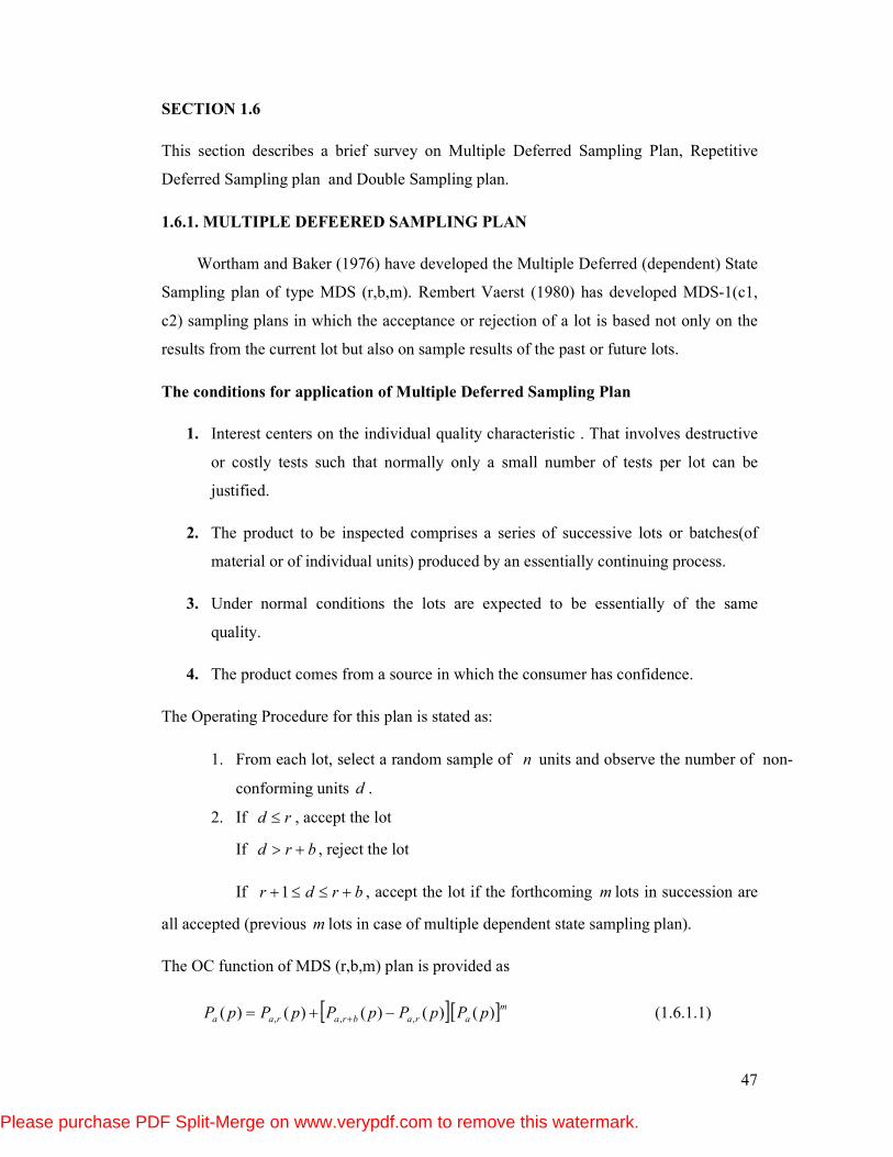
47

SECTION 1.6

This section describes a brief survey on Multiple Deferred Sampling Plan, Repetitive

Deferred Sampling plan and Double Sampling plan.

1.6.1. MULTIPLE DEFEERED SAMPLING PLAN

Wortham and Baker (1976) have developed the Multiple Deferred (dependent) State

Sampling plan of type MDS (r,b,m). Rembert Vaerst (1980) has developed MDS-1(c1,

c2) sampling plans in which the acceptance or rejection of a lot is based not only on the

results from the current lot but also on sample results of the past or future lots.

The conditions for application of Multiple Deferred Sampling Plan

1. Interest centers on the individual quality characteristic . That involves destructive

or costly tests such that normally only a small number of tests per lot can be

justified.

2. The product to be inspected comprises a series of successive lots or batches(of

material or of individual units) produced by an essentially continuing process.

3. Under normal conditions the lots are expected to be essentially of the same

quality.


The Operating Procedure for this plan is stated as:

1. From each lot, select a random sample of n units and observe the number of non-

conforming units d .

2. If rd ≤ , accept the lot

If brd +> , reject the lot

If brdr +≤≤+1 , accept the lot if the forthcoming m lots in succession are

all accepted (previous m lots in case of multiple dependent state sampling plan).

The OC function of MDS (r,b,m) plan is provided as

[ ][ ]marabraraa pPpPpPpPpP )()()()()( ,,, −+= + (1.6.1.1)


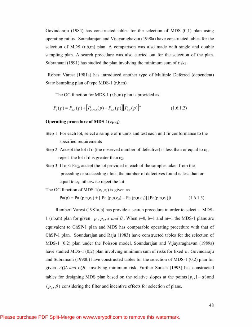
48

Govindaraju (1984) has constructed tables for the selection of MDS (0,1) plan using

operating ratios. Soundarajan and Vijayaraghavan (1990a) have constructed tables for the

selection of MDS (r,b,m) plan. A comparison was also made with single and double

sampling plan. A search procedure was also carried out for the selection of the plan.

Subramani (1991) has studied the plan involving the minimum sum of risks.

Robert Varest (1981a) has introduced another type of Multiple Deferred (dependent)

State Sampling plan of type MDS-1 (r,b,m).

The OC function for MDS-1 (r,b,m) plan is provided as

[ ][ ]mrarabraraa pPpPpPpPpP )()()()()( ,,,, −+= + (1.6.1.2)

Operating procedure of MDS-1(c1,c2)

Step 1: For each lot, select a sample of n units and test each unit fir conformance to the

specified requirements

Step 2: Accept the lot if d (the observed number of defective) is less than or equal to c1,

reject the lot if d is greater than c2.

Step 3: If c1<d<c2, accept the lot provided in each of the samples taken from the

preceding or succeeding i lots, the number of defectives found is less than or

equal to c1, otherwise reject the lot.

The OC function of MDS-1(c1,c2) is given as

Pa(p) = Pa (p,n,c1) + [ Pa (p,n,c2) – Pa (p,n,c1)].[Pa(p,n,c1)]i (1.6.1.3)

Rambert Varest (1981a,b) has provide a search procedure in order to select a MDS-

1 (r,b,m) plan for given βα andpp ,, 21 . When r=0, b=1 and m=1 the MDS-1 plans are

equivalent to ChSP-1 plan and MDS has comparable operating procedure with that of

ChSP-1 plan. Soundarajan and Raju (1983) have constructed tables for the selection of

MDS-1 (0,2) plan under the Poisson model. Soundarajan and Vijayaraghavan (1989a)

have studied MDS-1 (0,2) plan involving minimum sum of risks for fixed n . Govindaraju

and Subramani (1990b) have constructed tables for the selection of MDS-1 (0,2) plan for

given LQLandAQL involving minimum risk. Further Suresh (1993) has constructed

tables for designing MDS plan based on the relative slopes at the points )1,( 1 α−p and

),( 2 βp considering the filter and incentive effects for selection of plans.


49

1.6.2. REPETITIVE DEFERRED SAMPLING PLAN

The RDS plan was developed by Shankar and Mahopatra(1991) and this plan is

essentially an extension of the multiple Deferred Sampling plan MDS-(c1,c2) due to

Rambert Vaerst(1981).

In this plan, the acceptance or rejection of a lot in deferred state is dependent on

the inspection results of the preceding or succeeding lots under Repetitive Group

Sampling (RGS) inspection. RGS is the particular case of RDS plan. Further Wortham

and Baker (1976) have developed Multiple Deferred State sampling (MDS) plans and

provided tables for construct ion of plans.

Suresh (1993) has proposed procedures to select Multiple Deferred State Plan of

type MDS and MDS-1 indexed through producer and consumer quality levels considering

filter and incentive effect. Lilly Christina (1995) has given the procedure for the selection

of RDS plan with given acceptable quality levels and also compared RDS plan with RGS

plan with respect to operating ratio (OR) and ASN curve.

Saminathan (2005) has provided Selection through ratio of relative slopes for

Repetitive Deferred sampling plan and Multiple Repetitive Group sampling plan. The

relative slope of the OC curve at this point denoted as h* also be used to fix the

discrimination of the OC curve for any sampling plan.

Operating Procedure

1. Draw a random sample of size n from the lot and determine the number of

defectives (d).

2. Accept the lot if d≤c1 (or)Reject the lot if d>c2

3. If c1<d<c2, accept the lot provided “ i “ preceding or succeeding lots are

accepted under RGS inspection plan, otherwise reject the lot

Here c1 and c2 are acceptance number of RDS such that c1<c2. When i=1 this plan reduces

to RGS plan

The operating characteristic function Pa (p) of RDS plan is derived by Shankar

and Mahopatra (1991) using the Poisson model as

i

c

i

ac

i

ca

aP

PPPPpP

)1(

)1()(

−

+−= (1.6.2.1)


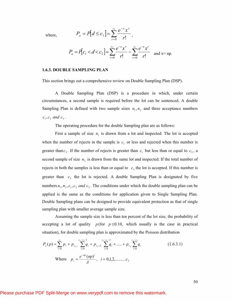
50

where, [ ] ∑=

−

=≤=1

0

1!

c

r

rx

ar

xecdPP ,

[ ] ∑∑=

−

=

−

−=<<=12

00

21!!

c

r

rxc

r

rx

ar

xe

r

xecdcPP and x= np.

1.6.3. DOUBLE SAMPLING PLAN

This section brings out a comprehensive review on Double Sampling Plan (DSP).

A Double Sampling Plan (DSP) is a procedure in which, under certain

circumstances, a second sample is required before the lot can be sentenced. A double

Sampling Plan is defined with two sample sizes 21 ,nn and three acceptance numbers

321 , candcc .

The operating procedure for the double Sampling plan are as follows:

First a sample of size 1n is drawn from a lot and inspected. The lot is accepted

when the number of rejects in the sample is 1c or less and rejected when this number is

greater than 2c . If the number of rejects is greater than 1c but less than or equal to 2c , a

second sample of size 2n is drawn from the same lot and inspected. If the total number of

rejects in both the samples is less than or equal to 3c the lot is accepted. If this number is

greater than 3c the lot is rejected. A double Sampling Plan is designated by five

numbers 32121 ,,, candccnn . The conditions under which the double sampling plan can be

applied is the same as the conditions for application given to Single Sampling Plan.

Double Sampling plans can be designed to provide equivalent protection as that of single

sampling plan with smaller average sample size.

Assuming the sample size is less than ten percent of the lot size, the probability of

accepting a lot of quality p (for ,10.0≤p which usually is the case in practical

situation), for double sampling plan is approximated by the Poisson distribution

∑∑∑∑−

=

−−

=+

−−

==

++++=+

23

2

13

1

13

11

1

0

2

0

2

1

00

.....)(cc

i

ic

cc

i

ic

cc

i

ic

c

i

ia qpqpqpppP (1.6.3.1)

Where 2.,.........2,1,0,!

)(ci

i

npep

inp

i ==−


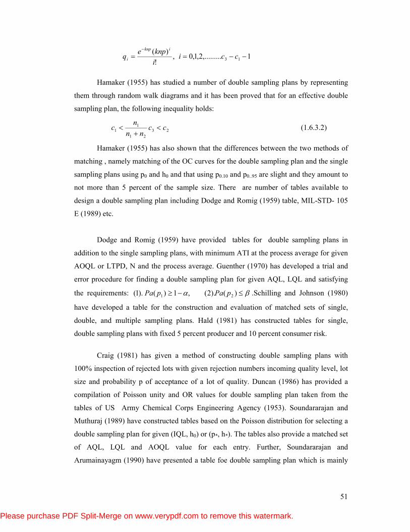
51

1,.........2,1,0,!

)(13 −−==

−

ccii

knpeq

iknp

i

Hamaker (1955) has studied a number of double sampling plans by representing

them through random walk diagrams and it has been proved that for an effective double

sampling plan, the following inequality holds:

23

21

11 cc

nn

nc <

+< (1.6.3.2)

Hamaker (1955) has also shown that the differences between the two methods of

matching , namely matching of the OC curves for the double sampling plan and the single

sampling plans using p0 and h0 and that using p0.10 and p0..95 are slight and they amount to

not more than 5 percent of the sample size. There are number of tables available to

design a double sampling plan including Dodge and Romig (1959) table, MIL-STD- 105

E (1989) etc.

Dodge and Romig (1959) have provided tables for double sampling plans in

addition to the single sampling plans, with minimum ATI at the process average for given

AOQL or LTPD, N and the process average. Guenther (1970) has developed a trial and

error procedure for finding a double sampling plan for given AQL, LQL and satisfying

the requirements: βα ≤−≥ )().2(,1)().1( 21 pPapPa .Schilling and Johnson (1980)

have developed a table for the construction and evaluation of matched sets of single,

double, and multiple sampling plans. Hald (1981) has constructed tables for single,

double sampling plans with fixed 5 percent producer and 10 percent consumer risk.

Craig (1981) has given a method of constructing double sampling plans with

100% inspection of rejected lots with given rejection numbers incoming quality level, lot

size and probability p of acceptance of a lot of quality. Duncan (1986) has provided a

compilation of Poisson unity and OR values for double sampling plan taken from the

tables of US Army Chemical Corps Engineering Agency (1953). Soundararajan and

Muthuraj (1989) have constructed tables based on the Poisson distribution for selecting a

double sampling plan for given (IQL, h0) or (p*, h*). The tables also provide a matched set

of AQL, LQL and AOQL value for each entry. Further, Soundararajan and

Arumainayagm (1990) have presented a table foe double sampling plan which is mainly


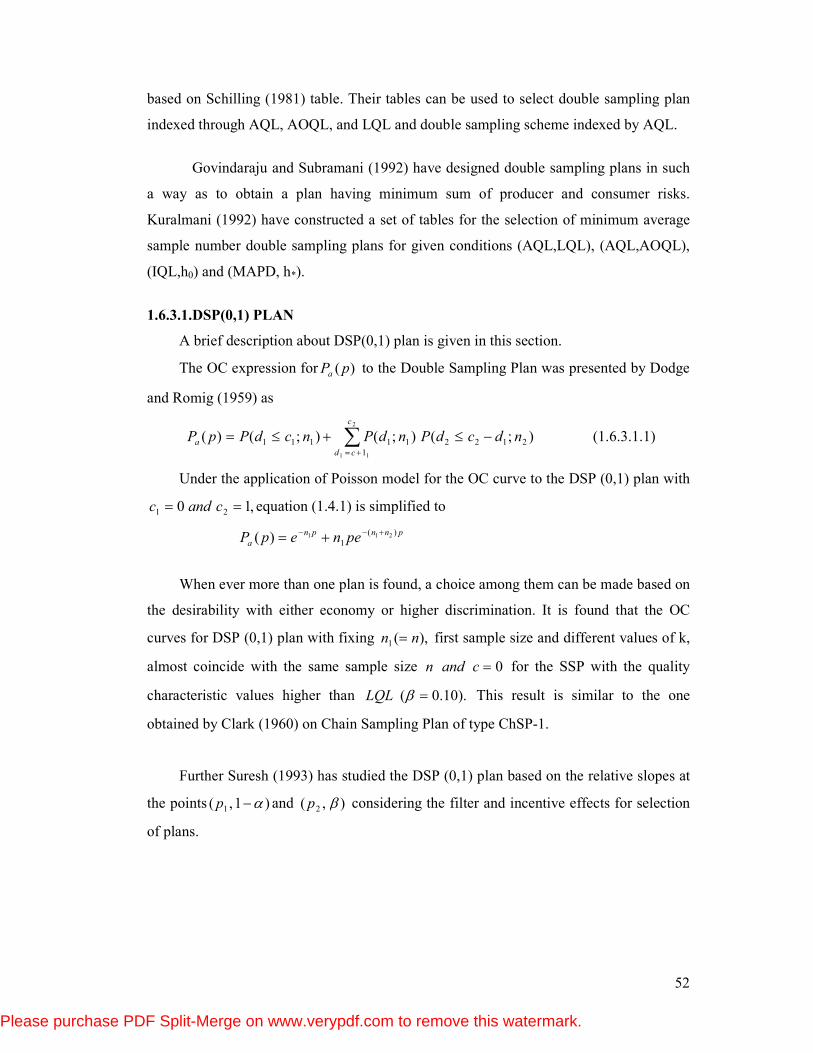
52

based on Schilling (1981) table. Their tables can be used to select double sampling plan

indexed through AQL, AOQL, and LQL and double sampling scheme indexed by AQL.

Govindaraju and Subramani (1992) have designed double sampling plans in such

a way as to obtain a plan having minimum sum of producer and consumer risks.

Kuralmani (1992) have constructed a set of tables for the selection of minimum average

sample number double sampling plans for given conditions (AQL,LQL), (AQL,AOQL),

(IQL,h0) and (MAPD, h*).

1.6.3.1.DSP(0,1) PLAN

A brief description about DSP(0,1) plan is given in this section.

The OC expression for )(pPa to the Double Sampling Plan was presented by Dodge

and Romig (1959) as

);();();()( 2122

1

11111

2

11

ndcdPndPncdPpP

c

cd

a −≤+≤= ∑+=

(1.6.3.1.1)

Under the application of Poisson model for the OC curve to the DSP (0,1) plan with

,10 21 == candc equation (1.4.1) is simplified to

pnnpn

a penepP)(

1211)(

+−− +=

When ever more than one plan is found, a choice among them can be made based on

the desirability with either economy or higher discrimination. It is found that the OC

curves for DSP (0,1) plan with fixing ),(1 nn = first sample size and different values of k,

almost coincide with the same sample size 0=candn for the SSP with the quality

characteristic values higher than ).10.0( =βLQL This result is similar to the one

obtained by Clark (1960) on Chain Sampling Plan of type ChSP-1.

Further Suresh (1993) has studied the DSP (0,1) plan based on the relative slopes at

the points )1,( 1 α−p and ),( 2 βp considering the filter and incentive effects for selection

of plans.


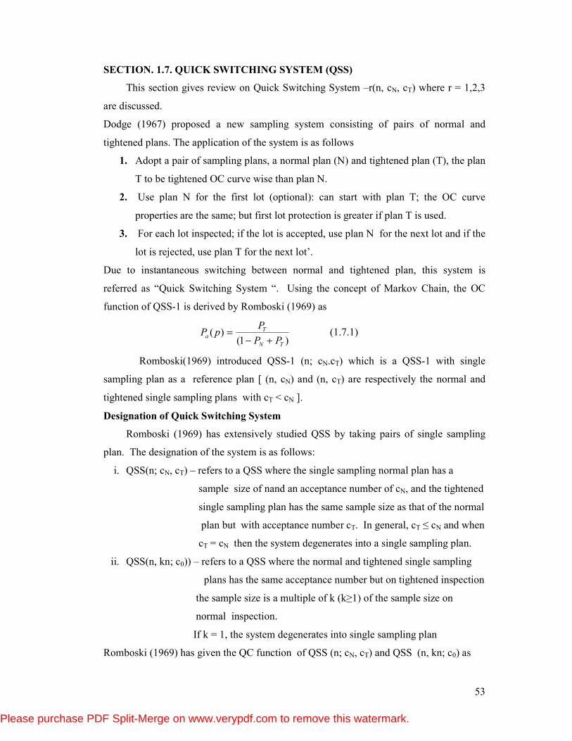
53

SECTION. 1.7. QUICK SWITCHING SYSTEM (QSS)

This section gives review on Quick Switching System –r(n, cN, cT) where r = 1,2,3

are discussed.

Dodge (1967) proposed a new sampling system consisting of pairs of normal and

tightened plans. The application of the system is as follows

1. Adopt a pair of sampling plans, a normal plan (N) and tightened plan (T), the plan

T to be tightened OC curve wise than plan N.

2. Use plan N for the first lot (optional): can start with plan T; the OC curve

properties are the same; but first lot protection is greater if plan T is used.

3. For each lot inspected; if the lot is accepted, use plan N for the next lot and if the

lot is rejected, use plan T for the next lot’.

Due to instantaneous switching between normal and tightened plan, this system is

referred as “Quick Switching System “. Using the concept of Markov Chain, the OC

function of QSS-1 is derived by Romboski (1969) as

)1(

)(TN

Ta

PP

PpP

+−= (1.7.1)

Romboski(1969) introduced QSS-1 (n; cN.cT) which is a QSS-1 with single

sampling plan as a reference plan [ (n, cN) and (n, cT) are respectively the normal and

tightened single sampling plans with cT < cN ].

Designation of Quick Switching System

Romboski (1969) has extensively studied QSS by taking pairs of single sampling

plan. The designation of the system is as follows:

i. QSS(n; cN, cT) – refers to a QSS where the single sampling normal plan has a

sample size of nand an acceptance number of cN, and the tightened

single sampling plan has the same sample size as that of the normal

plan but with acceptance number cT. In general, cT ≤ cN and when

cT = cN then the system degenerates into a single sampling plan.

ii. QSS(n, kn; c0)) – refers to a QSS where the normal and tightened single sampling

plans has the same acceptance number but on tightened inspection

the sample size is a multiple of k (k≥1) of the sample size on

normal inspection.

If k = 1, the system degenerates into single sampling plan

Romboski (1969) has given the QC function of QSS (n; cN, cT) and QSS (n, kn; c0) as


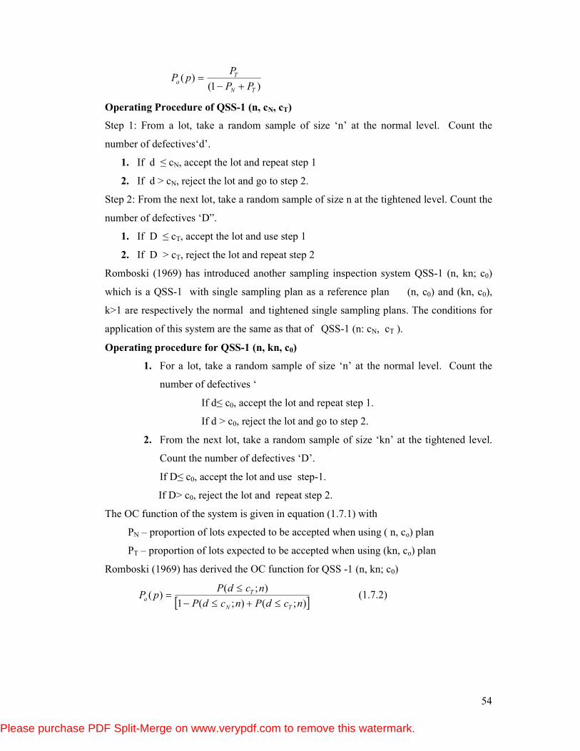
54

)1(

)(TN

Ta

PP

PpP

+−=

Operating Procedure of QSS-1 (n, cN, cT)

Step 1: From a lot, take a random sample of size ‘n’ at the normal level. Count the

number of defectives‘d’.

1. If d ≤ cN, accept the lot and repeat step 1

2. If d > cN, reject the lot and go to step 2.

Step 2: From the next lot, take a random sample of size n at the tightened level. Count the

number of defectives ‘D”.

1. If D ≤ cT, accept the lot and use step 1

2. If D > cT, reject the lot and repeat step 2

Romboski (1969) has introduced another sampling inspection system QSS-1 (n, kn; c0)

which is a QSS-1 with single sampling plan as a reference plan (n, c0) and (kn, c0),

k>1 are respectively the normal and tightened single sampling plans. The conditions for

application of this system are the same as that of QSS-1 (n: cN, cT ).

Operating procedure for QSS-1 (n, kn, c0)

1. For a lot, take a random sample of size ‘n’ at the normal level. Count the

number of defectives ‘

If d≤ c0, accept the lot and repeat step 1.

If d > c0, reject the lot and go to step 2.

2. From the next lot, take a random sample of size ‘kn’ at the tightened level.

Count the number of defectives ‘D’.

If D≤ c0, accept the lot and use step-1.

If D> c0, reject the lot and repeat step 2.

The OC function of the system is given in equation (1.7.1) with

PN – proportion of lots expected to be accepted when using ( n, co) plan

PT – proportion of lots expected to be accepted when using (kn, co) plan

Romboski (1969) has derived the OC function for QSS -1 (n, kn; c0)

[ ]);();(1

);()(

ncdPncdP

ncdPpP

TN

Ta ≤+≤−

≤= (1.7.2)


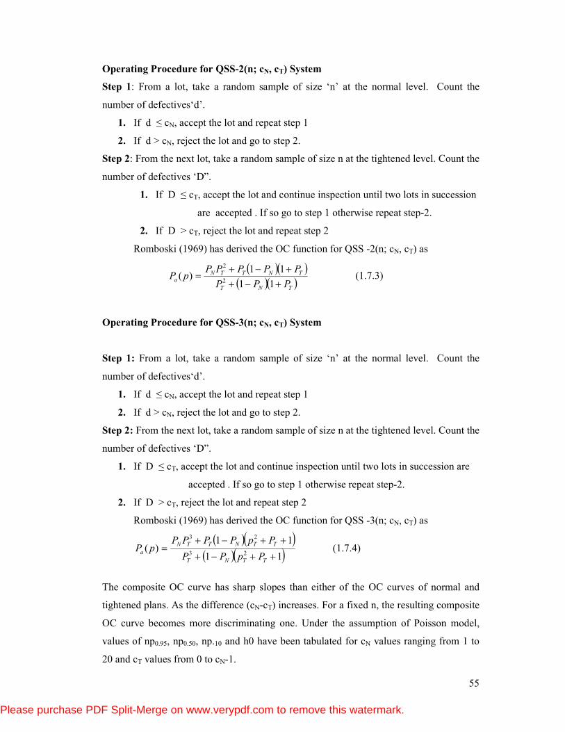
55

Operating Procedure for QSS-2(n; cN, cT) System







1. If D ≤ cT, accept the lot and continue inspection until two lots in succession

are accepted . If so go to step 1 otherwise repeat step-2.


Romboski (1969) has derived the OC function for QSS -2(n; cN, cT) as

( )( )

( )( )TNT

TNTTNa

PPP

PPPPPpP

+−+

+−+=

11

11)(

2

2

(1.7.3)

Operating Procedure for QSS-3(n; cN, cT) System







1. If D ≤ cT, accept the lot and continue inspection until two lots in succession are

accepted . If so go to step 1 otherwise repeat step-2.


Romboski (1969) has derived the OC function for QSS -3(n; cN, cT) as

( )( )( )( )11

11)(

23

23

++−+

++−+=

TTNT

TTNTTN

aPpPP

PpPPPPpP (1.7.4)

The composite OC curve has sharp slopes than either of the OC curves of normal and

tightened plans. As the difference (cN-cT) increases. For a fixed n, the resulting composite

OC curve becomes more discriminating one. Under the assumption of Poisson model,

values of np0.95, np0.50, np.10 and h0 have been tabulated for cN values ranging from 1 to

20 and cT values from 0 to cN-1.


56

Operating procedure for QSS -2(n, kn, c0)

1. For a lot, take a random sample of size ‘n’ at the normal level. Count the number

of defectives ‘

If d≤ c0, accept the lot and repeat step 1.

If d > c0, reject the lot and go to step 2

2. From the next lot, take a random sample of size ‘kn’ at the tightened level. Count

the number of defectives ‘D’.

3. If D≤ c0, accept the lot and continue inspection until two lots in succession are

accepted . If so go to step 1 otherwise repeat step-2.

4. If D> c0, reject the lot and repeat step 2.

Operating procedure for QSS -3(n, kn, c0)

The operating procedure of QSS-3(n, kn; c0) is same as that of QSS-2(n, kn; c0)

except for the step 2(i), which is to be read as follows:

Step 2(i): If D≤ c0, accept the lot and continue inspection until three lots in succession are

accepted. If so go to step 1 of QSS-2 (n, kn; c0) ,otherwise repeat step-2.

The number of QSS-1((n; cN, cT) have been matched to single sampling plan using

operating ratio and it has been shown that a considerable reduction in sample size relative

to single sampling plan, can be achieved by using QSS-1 without any significant decrease

in sampling performance. Similarly QSS-1 has been matched to certain chain sampling

plans[ChSP(n; k1, k2, c1, c2)] of Dodge and Stephens(1964) and it has been shown that

QSS-1 is not as efficient as the matched chain sampling plan.


57

SECTION. 1.8 : BAYESIAN SAMPLING PLANS

This section includes Bayesian Sampling Plans such as Bayesian Repetitive Group

Sampling Plan, Bayesian Multiple deferred Sampling plan, Bayesian Chain Sampling

Plan and Bayesian Skip-lot Sampling Plan.

1.8.1. BAYESIAN REPETITIVE GROUP SAMPLING PLAN

Conditions for Application:

The conditions for application for RGS plan are given below:

1. The size of the lot is taken to be sufficiently large

2. Under normal conditions the lots are expected to be of essentially the same quality

(expressed in percent defective).


Procedure for Operating Characteristic function:

Step 1. Take a random sample of size n.

Step 2. Count the number of defectives d, in the sample.

Step 3. If d ≤ c1, accept the lot.

If d > c2, reject the lot.

If c1 < d ≤ c2, repeat steps 1, 2 and 3.

The RGS plans are characterized by 3 parameters namely n, c1 and c2. When c1=c2 the

resulting plan is the usual single sampling plan.

The operating characteristic function of RGS is obtained by Sherman [1965] as

)()(

)()(

pPpP

pPpP

ra

a

A += (1.8.1.1)

Where Pa(p) be the probability of acceptance in a particular group sample, Pr(p) be the

probability of rejection in a particular group sample.


58

The probability density function for the Gamma distribution with parameters α and β is

≥≥≥

Γ=Γ

−−

otherwise

ppe

p

p

,0

0,0,0,),/(

1

βαα

ββα

ααβ

(1.8.1.2)

Suppose that the defects per unit in the submitted lots p can be modeled with Gamma

Distribution having parameters α and β.

For any RGS plan, the probability of eventually accepting the lot is given as

)('

11

1

PP

PPa

+= (1.8.1.3)

where P1 is the Probability of acceptance and P1’ is the probability of rejection.

The probability of acceptance in a particular group sample is

∑=

−

=1

1

1

0 1

1!

)()(

c

k

knp

k

npepP (1.8.1.4)

The probability of rejection in a particular group sample is

∑∞

=

−

=22

2

!

)()('

2

1

ck

knp

k

npepP (1.8.1.5)

The OC function of RGS plan is

∑

∑

+=

−

=

−

−

=2

12

2

1

1

1

1 2

0 1

!

)(1

!

)(

c

ck

knp

c

k

knp

a

k

npe

k

npe

P (1.8.1.6)

Let p has a prior distribution with density function given as

00,),(/)( 1 >>Γ= −− pandtsstpepw sspt (1.8.1.7)

with parameters s and t and mean, )(/ saytsp µ== .

The APA function is given as


59

)8.1.8.1(........................................

))()3("!!/)((

))()3()!(!/)2((

)()2(!!/)(

))()(!/)((

)(

"

221

0 1

"

221

"

22

21

0 1

21

2

21

0 1

21

1

01

11

221

1

1

2

12'

1

221

21

1

1

2

12

21

21

1

1

2

12

21

11

+

Γ++++Γ+

Γ+++Γ+

Γ+++Γ+

Γ++Γ=

=

+++

= +=≠

+

++

= +=

+

++

= +=

+

=

+

∑ ∑

∑ ∑

∑ ∑

∑

∫

stnkkkkkkstn

stnkkkkstn

stnkkkkstn

stnkkstn

dppwPP

kkksc

k

c

ckk

skkk

kksc

k

c

ck

skk

kksc

k

c

ck

skk

c

k

kssk

a

In particular, the average probability of acceptance for c1=0, c2=1 is obtained as follows:

∑∞

=

−+− Γ+−+Γ=0

11)()/()1(),/)1,0,((

k

ksksstknksnttsnP

(1.8.1.9)

1.8.2. BAYESIAN MULTIPLE DEFERRED STATE SAMPLING PLAN

Wortham and Baker(1976) developed the multiple deferred and multiple

dependent state sampling plans. These plans are designated as MDS(r,b).

Bayesian Multiple Deferred State Sampling Plan (BMDS(r , b))

The probability density function with Gamma prior distribution, having

parameters s and t is,

Otherwise

ptsstpetspw sspt

0

0,0,),(/),;( 1

=

>>Γ= −−

(1.8.2.1)

Let the defects per unit in the submitted lot p, is modeled by a Gamma distribution

with parameters s and t. If these lots are subjected to a MDS(0,1) and with parameters n

and m for a fixed value of p, then the proportion of lots expected to be accepted with

operating characteristic function defined by MDS(0,1) is

npeepmnP mnpnp )1()/,( +−− += (1.8.2.2)


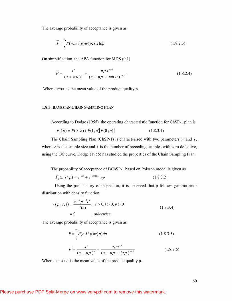
60

The average probability of acceptance is given as

∫∞

=0

),;()/,( dptspwpmnPP (1.8.2.3)

On simplification, the APA function for MDS (0,1)

1

1

)()( +

+

+++

+=

s

s

s

s

mnns

sn

ns

sP

µµµ

µ (1.8.2.4)

Where µ=s/t, is the mean value of the product quality p.

1.8.3. BAYESIAN CHAIN SAMPLING PLAN

According to Dodge (1955) the operating characteristic function for ChSP-1 plan is

[ ]ia nPnPnPpP );0();1();0()( += (1.8.3.1)

The Chain Sampling Plan (ChSP-1) is characterized with two parameters n and i ,

where n is the sample size and i is the number of preceding samples with zero defective,

using the OC curve, Dodge (1955) has studied the properties of the Chain Sampling Plan.

The probability of acceptance of BChSP-1 based on Poisson model is given as

npeepinP inpnp

a

)1()/,( +−− += (1.8.3.2)

Using the past history of inspection, it is observed that p follows gamma prior

distribution with density function,

otherwise

ptss

tpetspw

sspt

,0

0,0,0,)(

),;(1

=

>>>Γ

=−−

(1.8.3.4)

The average probability of acceptance is given as

∫∞

=0

)()/,( dppwpinPP (1.8.3.5)

1

1

)()( +

+

+++

+=

s

s

s

s

inns

sn

ns

sP

µµµ

µ (1.8.3.6)

Where µ = s / t, is the mean value of the product quality p.


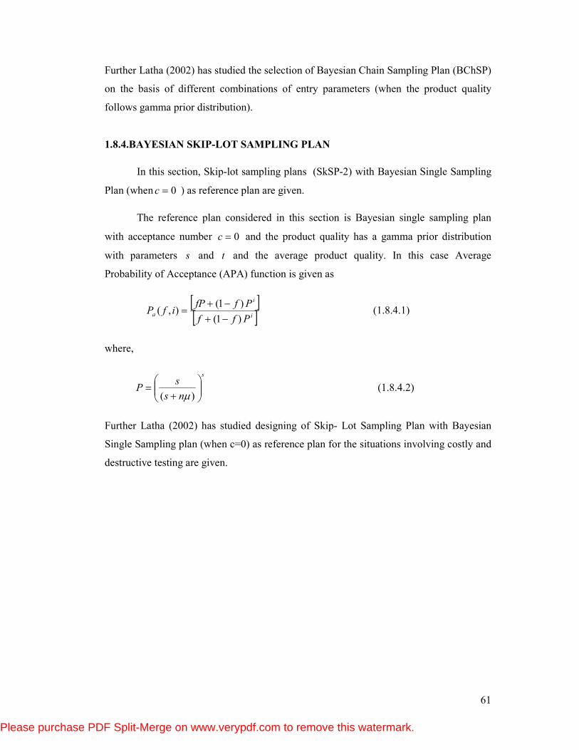
61

Further Latha (2002) has studied the selection of Bayesian Chain Sampling Plan (BChSP)

on the basis of different combinations of entry parameters (when the product quality

follows gamma prior distribution).

1.8.4.BAYESIAN SKIP-LOT SAMPLING PLAN

In this section, Skip-lot sampling plans (SkSP-2) with Bayesian Single Sampling

Plan (when 0=c ) as reference plan are given.

The reference plan considered in this section is Bayesian single sampling plan

with acceptance number 0=c and the product quality has a gamma prior distribution

with parameters s and t and the average product quality. In this case Average

Probability of Acceptance (APA) function is given as

[ ][ ]i

i

aPff

PffPifP

)1(

)1(),(

−+

−+= (1.8.4.1)

where,

s

ns

sP

+=

)( µ (1.8.4.2)

Further Latha (2002) has studied designing of Skip- Lot Sampling Plan with Bayesian

Single Sampling plan (when c=0) as reference plan for the situations involving costly and

destructive testing are given.


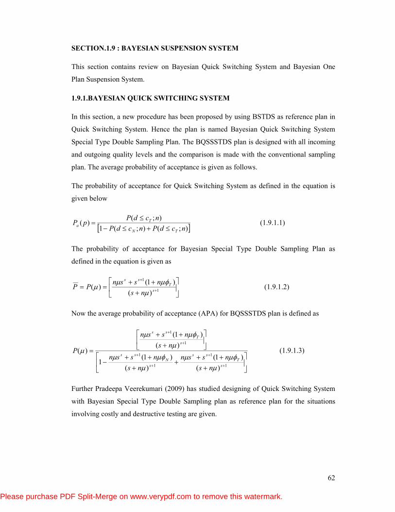
62

SECTION.1.9 : BAYESIAN SUSPENSION SYSTEM

This section contains review on Bayesian Quick Switching System and Bayesian One

Plan Suspension System.

1.9.1.BAYESIAN QUICK SWITCHING SYSTEM

In this section, a new procedure has been proposed by using BSTDS as reference plan in

Quick Switching System. Hence the plan is named Bayesian Quick Switching System

Special Type Double Sampling Plan. The BQSSSTDS plan is designed with all incoming

and outgoing quality levels and the comparison is made with the conventional sampling

plan. The average probability of acceptance is given as follows.

The probability of acceptance for Quick Switching System as defined in the equation is

given below

[ ]);();(1

);()(

ncdPncdP

ncdPpP

TN

Ta ≤+≤−

≤= (1.9.1.1)

The probability of acceptance for Bayesian Special Type Double Sampling Plan as

defined in the equation is given as

+

++==

+

+

1

1

)(

)1()(

s

T

ss

ns

nssnPP

µµφµ

µ (1.9.1.2)

Now the average probability of acceptance (APA) for BQSSSTDS plan is defined as

+

+++

+

++−

+

++

=

+

+

+

+

+

+

1

1

1

1

1

1

)(

)1(

)(

)1(1

)(

)1(

)(

s

T

ss

s

N

ss

s

T

ss

ns

nssn

ns

nssn

ns

nssn

P

µµφµ

µµφµ

µµφµ

µ (1.9.1.3)

Further Pradeepa Veerekumari (2009) has studied designing of Quick Switching System

with Bayesian Special Type Double Sampling plan as reference plan for the situations

involving costly and destructive testing are given.


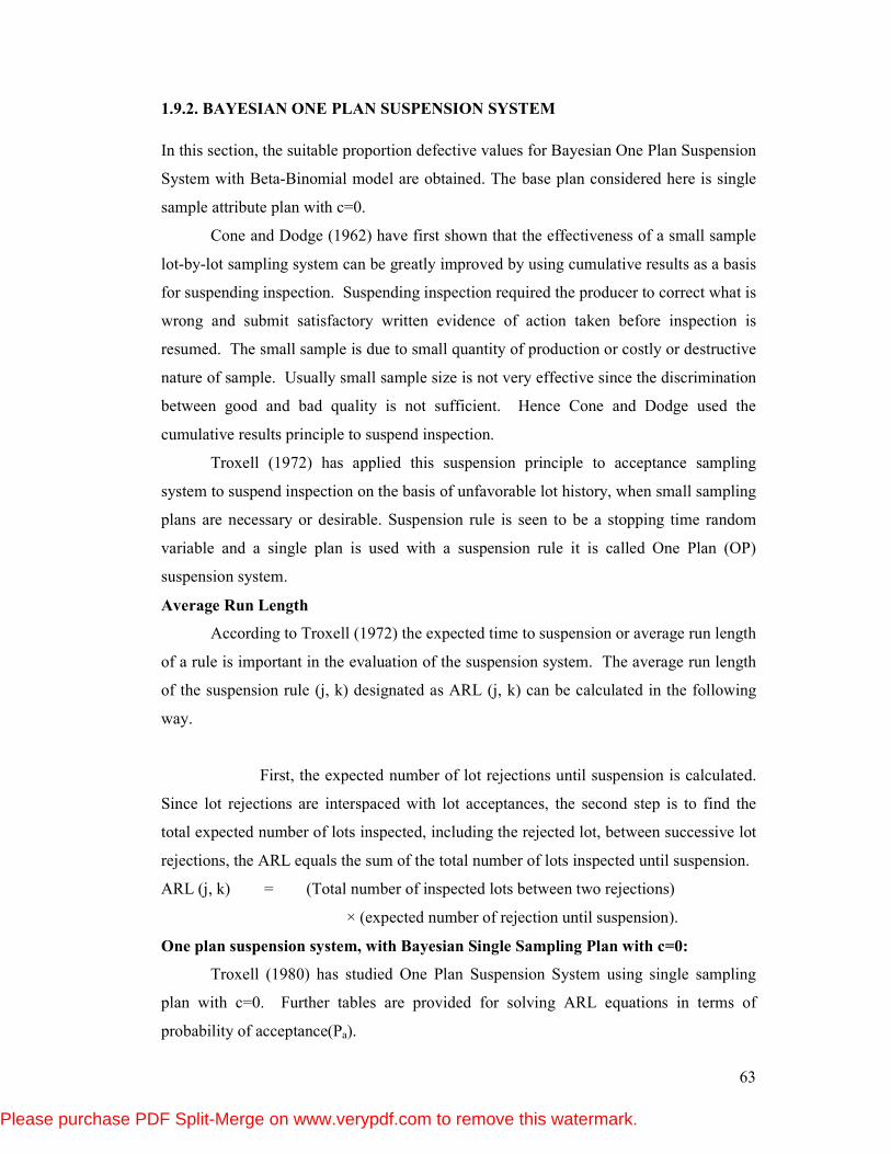
63

1.9.2. BAYESIAN ONE PLAN SUSPENSION SYSTEM

In this section, the suitable proportion defective values for Bayesian One Plan Suspension

System with Beta-Binomial model are obtained. The base plan considered here is single

sample attribute plan with c=0.

Cone and Dodge (1962) have first shown that the effectiveness of a small sample

lot-by-lot sampling system can be greatly improved by using cumulative results as a basis

for suspending inspection. Suspending inspection required the producer to correct what is

wrong and submit satisfactory written evidence of action taken before inspection is

resumed. The small sample is due to small quantity of production or costly or destructive

nature of sample. Usually small sample size is not very effective since the discrimination

between good and bad quality is not sufficient. Hence Cone and Dodge used the

cumulative results principle to suspend inspection.

Troxell (1972) has applied this suspension principle to acceptance sampling

system to suspend inspection on the basis of unfavorable lot history, when small sampling

plans are necessary or desirable. Suspension rule is seen to be a stopping time random

variable and a single plan is used with a suspension rule it is called One Plan (OP)

suspension system.

Average Run Length

According to Troxell (1972) the expected time to suspension or average run length

of a rule is important in the evaluation of the suspension system. The average run length

of the suspension rule (j, k) designated as ARL (j, k) can be calculated in the following

way.

First, the expected number of lot rejections until suspension is calculated.

Since lot rejections are interspaced with lot acceptances, the second step is to find the

total expected number of lots inspected, including the rejected lot, between successive lot

rejections, the ARL equals the sum of the total number of lots inspected until suspension.

ARL (j, k) = (Total number of inspected lots between two rejections)

× (expected number of rejection until suspension).

One plan suspension system, with Bayesian Single Sampling Plan with c=0:

Troxell (1980) has studied One Plan Suspension System using single sampling

plan with c=0. Further tables are provided for solving ARL equations in terms of

probability of acceptance(Pa).


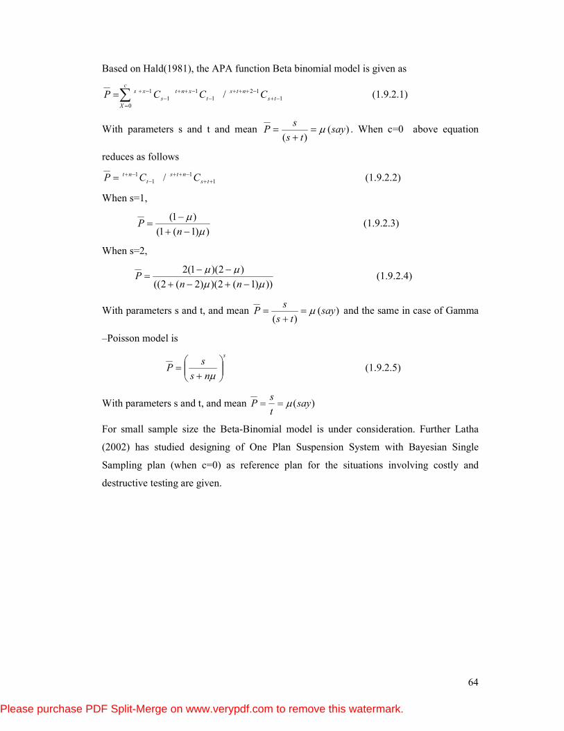
64

Based on Hald(1981), the APA function Beta binomial model is given as

1

12

1

1

1

1

0

/ −+−+++

−−++

−−+

=∑= ts

nts

t

xnt

s

xc

X

s CCCP (1.9.2.1)

With parameters s and t and mean )()(

sayts

sP µ=

+= . When c=0 above equation

reduces as follows

1

1

1

1 / ++−++

−−+= ts

nts

t

nt CCP (1.9.2.2)

When s=1,

))1(1(

)1(

µµ−+

−=

nP (1.9.2.3)

When s=2,

)))1(2)()2(2((

)2)(1(2

µµµµ

−+−+−−

=nn

P (1.9.2.4)

With parameters s and t, and mean )()(

sayts

sP µ=

+= and the same in case of Gamma

–Poisson model is

s

ns

sP

+

=µ

(1.9.2.5)

With parameters s and t, and mean )(sayt

sP µ==

For small sample size the Beta-Binomial model is under consideration. Further Latha

(2002) has studied designing of One Plan Suspension System with Bayesian Single

Sampling plan (when c=0) as reference plan for the situations involving costly and

destructive testing are given.


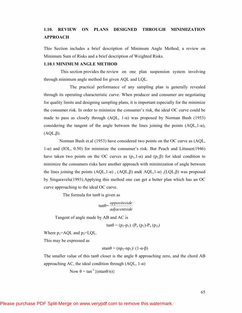
65

1.10. REVIEW ON PLANS DESIGNED THROUGH MINIMIZATION

APPROACH

This Section includes a brief description of Minimum Angle Method, a review on

Minimum Sum of Risks and a brief description of Weighted Risks.

1.10.1 MINIMUM ANGLE METHOD

This section provides the review on one plan suspension system involving

through minimum angle method for given AQL and LQL.

The practical performance of any sampling plan is generally revealed

through its operating characteristic curve. When producer and consumer are negotiating

for quality limits and designing sampling plans, it is important especially for the minimize

the consumer risk. In order to minimize the consumer’s risk, the ideal OC curve could be

made to pass as closely through (AQL, 1-α) was proposed by Norman Bush (1953)

considering the tangent of the angle between the lines joining the points (AQL,1-α),

(AQL,β).

Norman Bush et.al (1953) have considered two points on the OC curve as (AQL,

1-α) and (IOL, 0.50) for minimize the consumer’s risk. But Peach and Littauer(1946)

have taken two points on the OC curves as (p1,1-α) and (p2,β) for ideal condition to

minimize the consumers risks here another approach with minimization of angle between

the lines joining the points (AQL,1-α) , (AQL,β) and( AQL,1-α) ,(LQL,β) was proposed

by Singaravelu(1993).Applying this method one can get a better plan which has an OC

curve approaching to the ideal OC curve.

The formula for tanθ is given as

tanθ=deadjacentsi

deoppositesi

Tangent of angle made by AB and AC is

tanθ = (p2-p1)/ (Pa (p1)-Pa (p2))

Where p1=AQL and p2=LQL.

This may be expressed as

ntanθ = (np2-np1)/ (1-α-β)

The smaller value of this tanθ closer is the angle θ approaching zero, and the chord AB

approaching AC, the ideal condition through (AQL, 1-α)

Now θ = tan-1{(ntanθ/n)}


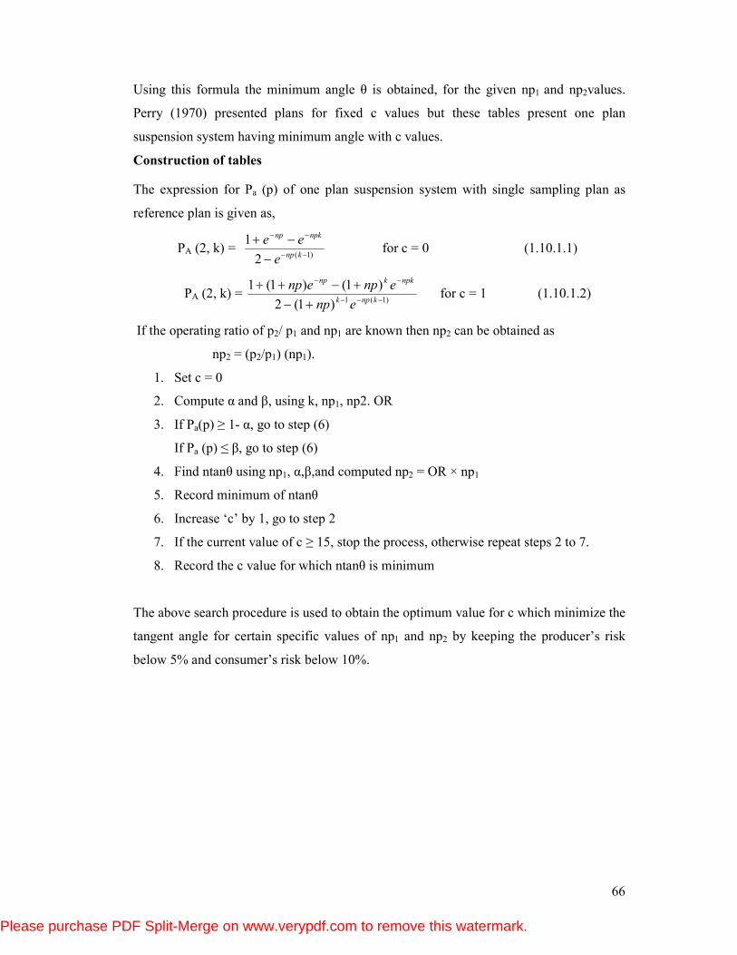
66

Using this formula the minimum angle θ is obtained, for the given np1 and np2values.

Perry (1970) presented plans for fixed c values but these tables present one plan

suspension system having minimum angle with c values.

Construction of tables

The expression for Pa (p) of one plan suspension system with single sampling plan as

reference plan is given as,

PA (2, k) = )1(2

1−−

−−

−

−+knp

npknp

e

ee for c = 0 (1.10.1.1)

PA (2, k) = )1(1)1(2

)1()1(1−−−

−−

+−

+−++knpk

npkknp

enp

enpenp for c = 1 (1.10.1.2)

If the operating ratio of p2/ p1 and np1 are known then np2 can be obtained as

np2 = (p2/p1) (np1).

1. Set c = 0

2. Compute α and β, using k, np1, np2. OR

3. If Pa(p) ≥ 1- α, go to step (6)

If Pa (p) ≤ β, go to step (6)

4. Find ntanθ using np1, α,β,and computed np2 = OR × np1

5. Record minimum of ntanθ

6. Increase ‘c’ by 1, go to step 2

7. If the current value of c ≥ 15, stop the process, otherwise repeat steps 2 to 7.

8. Record the c value for which ntanθ is minimum

The above search procedure is used to obtain the optimum value for c which minimize the

tangent angle for certain specific values of np1 and np2 by keeping the producer’s risk

below 5% and consumer’s risk below 10%.


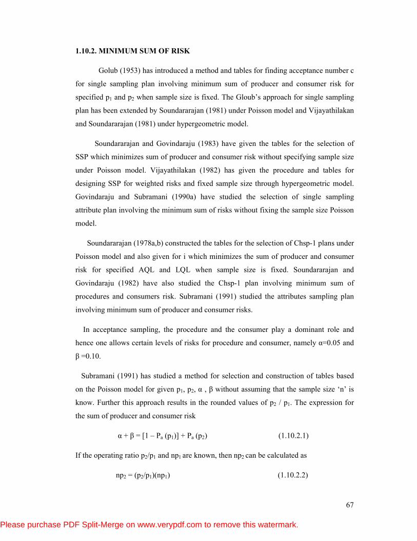
67

1.10.2. MINIMUM SUM OF RISK

Golub (1953) has introduced a method and tables for finding acceptance number c

for single sampling plan involving minimum sum of producer and consumer risk for

specified p1 and p2 when sample size is fixed. The Gloub’s approach for single sampling

plan has been extended by Soundararajan (1981) under Poisson model and Vijayathilakan

and Soundararajan (1981) under hypergeometric model.

Soundararajan and Govindaraju (1983) have given the tables for the selection of

SSP which minimizes sum of producer and consumer risk without specifying sample size

under Poisson model. Vijayathilakan (1982) has given the procedure and tables for

designing SSP for weighted risks and fixed sample size through hypergeometric model.

Govindaraju and Subramani (1990a) have studied the selection of single sampling

attribute plan involving the minimum sum of risks without fixing the sample size Poisson

model.

Soundararajan (1978a,b) constructed the tables for the selection of Chsp-1 plans under

Poisson model and also given for i which minimizes the sum of producer and consumer

risk for specified AQL and LQL when sample size is fixed. Soundararajan and

Govindaraju (1982) have also studied the Chsp-1 plan involving minimum sum of

procedures and consumers risk. Subramani (1991) studied the attributes sampling plan

involving minimum sum of producer and consumer risks.

In acceptance sampling, the procedure and the consumer play a dominant role and

hence one allows certain levels of risks for procedure and consumer, namely α=0.05 and

β =0.10.

Subramani (1991) has studied a method for selection and construction of tables based

on the Poisson model for given p1, p2, α , β without assuming that the sample size ‘n’ is

know. Further this approach results in the rounded values of p2 / p1. The expression for

the sum of producer and consumer risk

α + β = [1 – Pa (p1)] + Pa (p2) (1.10.2.1)

If the operating ratio p2/p1 and np1 are known, then np2 can be calculated as

np2 = (p2/p1)(np1) (1.10.2.2)


68

Advantages of using this approach are as follows:

• The plans tabulated have realistic operating ratios which are commonly

encountered in practice

• The OC curves of such plans will have a better ‘shoulder’

When the ‘producer’ and ‘consumer’ belong to the same company or interest, the sum of

risks may be minimized rather than fixing them at given levels.

1.10.3. WEIGHTED RISK

This section provides the review on one plan suspension system involving through

weighted risks.

Single sampling attributes plans have been developed for the situations where one

of the parameters either the sample size n or the acceptance number c is prefixed. The

method of obtaining this plan was in to minimize the sum of the producer risk and the

consumer risk.

When the sum of the risk is minimized, the individual values of the producer and

consumer risk are not taken into account and as such the resulting plan may be unduly

disadvantaged to one of them.

If the interest is only in the risk for the consumer, this risk can be fixed and a plan

with a fixed parameter which gives a risk equal to or nearly equal to the fixed consumer’s

risk can be obtained. But there may be plans for which the consumer’s risk is even

smaller than the fixed quantity and still not very unkind to the producer. By fixing the

consumer’s risk and obtaining a plan, this possibility is ruled out.

Another methods is to minimize the sum of the risks with different weights for the

producer risk and the consumer risk .when the sum is minimized both risks are given

equal weights. If the interest is in consumer risk, a larger weight can be assigned to the

consumer’s risk than the producer risk. Suppose w1 and w2 are the weights such that (w1 +

w2=1), then (w1 α + w2 β) can be minimized to obtain the necessary plan / system.

Minimizing w1 (α + w2 β) is the same as minimizing α + (w2/w1) β (w2/w1) can be

referred to as the index of the relative importance given to the consumers risk in

comparison with the producer’s risk and will be denoted by w.

When w is greater than one, the system obtained will be more favorable to the

consumer compared to equal weights system. When w is less than one, it will be more


69

favorable to the producer than the equal weight system. Systems which minimize the sum

of the weighted risks with fixed acceptance numbers are derived for the Binomial,

Poisson and Hypergeometric models.

Fixed Sample Size:

For the Poisson model the expression is

−−

− ∑∑

==

]!/))(1(exp[]!/))((exp[ 1

0

22

0

rnpnpwrnpnpwr

c

r

rc

r

(1.10.3.1)

which on imposing conditions yield ,

(p2 /p1)c < 1/w exp [n (p2 - p1)]<(p2 – p1)

c+1

And on simplification give the value of c as the integral part of

)/ln(

(

)/ln(

)ln(

12

)12

12

1

pp

ppn

pp

w −+

−

(1.10.3.2)

The value of c obtained here is different from the value obtained by Soundarajan (1971)

only by the term )/ln(

)ln(

12

1

pp

w−

which is zero when w =1 , reduces the value of c when w > 1

and increases the values of c when w <1 as in the case of binomial model.

Expressing the condition that (1.1.3.2) is not less than zero and is less than n always , the

tolerance limits for w have been obtained in terms of p1, p2 and n as

exp [ n (p2 – p1)] (p1/p2)n < w < exp [n(p2 – p1)]

Tables of binomial model are similar to those obtained for the Poisson model with fixed

n = 5, 10, 20, 25,40 and 50.

Fixed Acceptance Number:

The technique for obtaining the value of n which minimizes (w1α + w2β) using

Poisson model, one use the method of differential calculus and expression

∑=

−−=c

r

np0

exp(1)( µ) µr/r! +w ∂−∑

=

c

r 0

exp( µ) (∂ µ)r/r!

and obtain n as the integer nearest to


70

)(

)/ln()1(

)(

)ln(

12

12

12 pp

ppc

pp

w

−

++

− (1.10.3.3)

This expression differs from the expression for equal weights in In( w) /p2-p1 and as (p2

– p1) is always greater than zero , the value of n given by increases for w>1 and decreases

for w<1.

The lower limit for the value of w is obtained by setting (1.10.3.3) greater than or equal

to (c+1) and is given by,

[ ] )1(

2112 )/())(1(exp +−+≥ cppppcw (1.10.3.4)

Since (c + 1) (p2 – p1) is always positive, the lower limit for the value of w in the

Poisson model is always higher than the corresponding lower limit of w for the Binomial

model.

1.11. REVIEW ON PLANS DESIGNED THROUGH QUALITY REGIONS

This section provides the review on single sampling plan involving through Quality

Regions

This section introduces a method for designing Single Sampling Plan based on

range of quality instead of point-wise description of quality by invoking a novel approach

called the Quality Interval Sampling (QIS) plan. This method seems to be versatile and

can be adopted in the elementary production process where the stipulated quality level is

advisable to fix at later stage and provides a new concept for designing single sampling

plan involving quality levels. The sampling plans provide the vendor and buyer decision

rules for the product acceptance to meet the preset product quality requirement. Due to

rapid advancement of manufacturing technology, suppliers require their products to be of

high quality with very low fraction defectives often measured in parts per million.

Unfortunately, traditional methods in some particular situations fail to find out a minute

defect in the product. In order to overcome such problems Quality Interval Sampling

(QIS) plan is introduced. This section designs the parameters for the plan indexed with

Quality Regions. Technical terms are defined as in ANSI/ASQC Standards (1987).


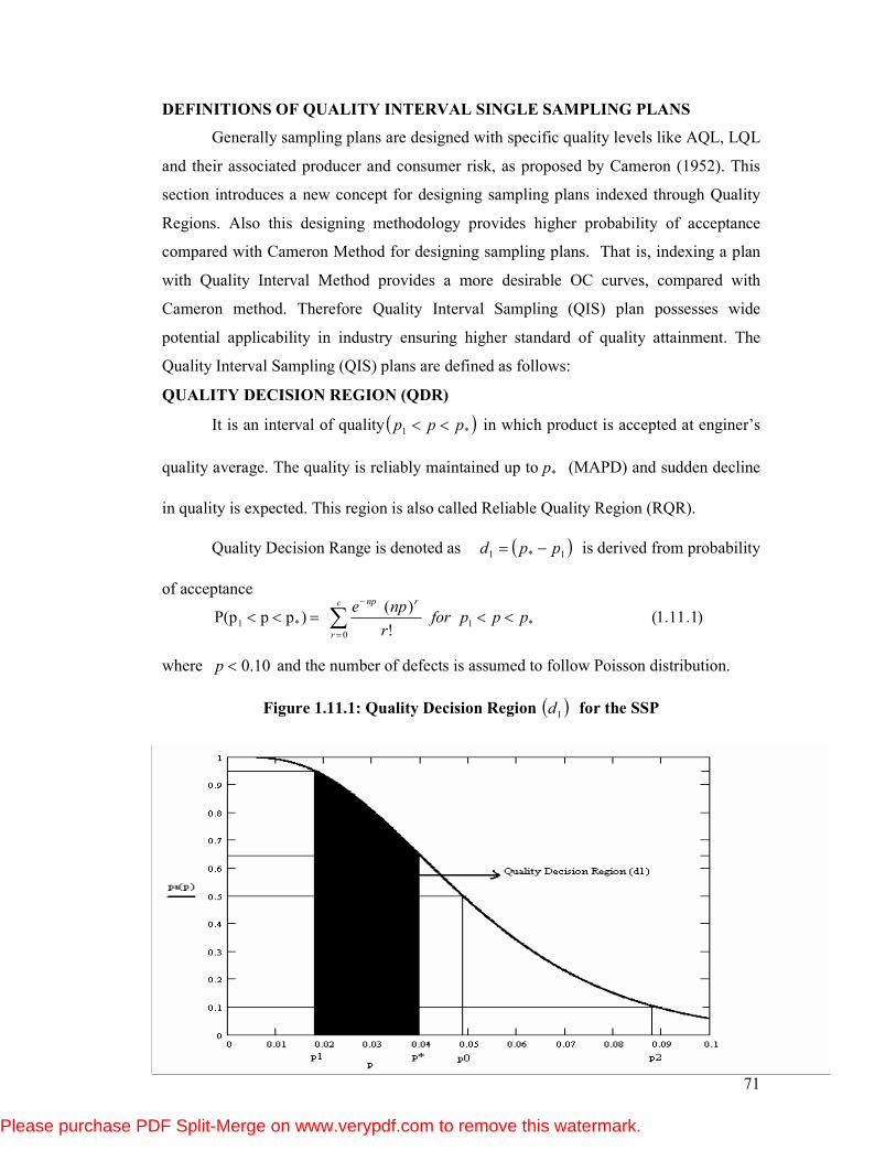
71

DEFINITIONS OF QUALITY INTERVAL SINGLE SAMPLING PLANS

Generally sampling plans are designed with specific quality levels like AQL, LQL

and their associated producer and consumer risk, as proposed by Cameron (1952). This

section introduces a new concept for designing sampling plans indexed through Quality

Regions. Also this designing methodology provides higher probability of acceptance

compared with Cameron Method for designing sampling plans. That is, indexing a plan

with Quality Interval Method provides a more desirable OC curves, compared with

Cameron method. Therefore Quality Interval Sampling (QIS) plan possesses wide

potential applicability in industry ensuring higher standard of quality attainment. The

Quality Interval Sampling (QIS) plans are defined as follows:

QUALITY DECISION REGION (QDR)

It is an interval of quality ( )*1 ppp << in which product is accepted at enginer’s

quality average. The quality is reliably maintained up to *p (MAPD) and sudden decline

in quality is expected. This region is also called Reliable Quality Region (RQR).

Quality Decision Range is denoted as ( )1*1 ppd −= is derived from probability

of acceptance

where 10.0<p and the number of defects is assumed to follow Poisson distribution.

Figure 1.11.1: Quality Decision Region ( )1d for the SSP

)1.11.1(!

)( )ppP(p *1

0

*1 pppforr

npec

r

rnp

<<=<< ∑=

−


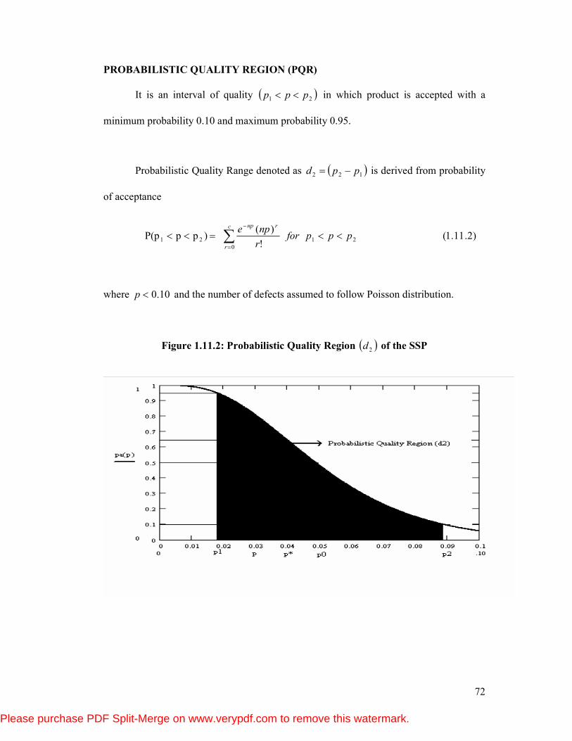
72

PROBABILISTIC QUALITY REGION (PQR)

It is an interval of quality ( )21 ppp << in which product is accepted with a

minimum probability 0.10 and maximum probability 0.95.

Probabilistic Quality Range denoted as ( )122 ppd −= is derived from probability

of acceptance

where 10.0<p and the number of defects assumed to follow Poisson distribution.

Figure 1.11.2: Probabilistic Quality Region ( )2d of the SSP

)2.11.1(!

)( )ppP(p 21

0

21 pppforr

npec

r

rnp

<<=<< ∑=

−


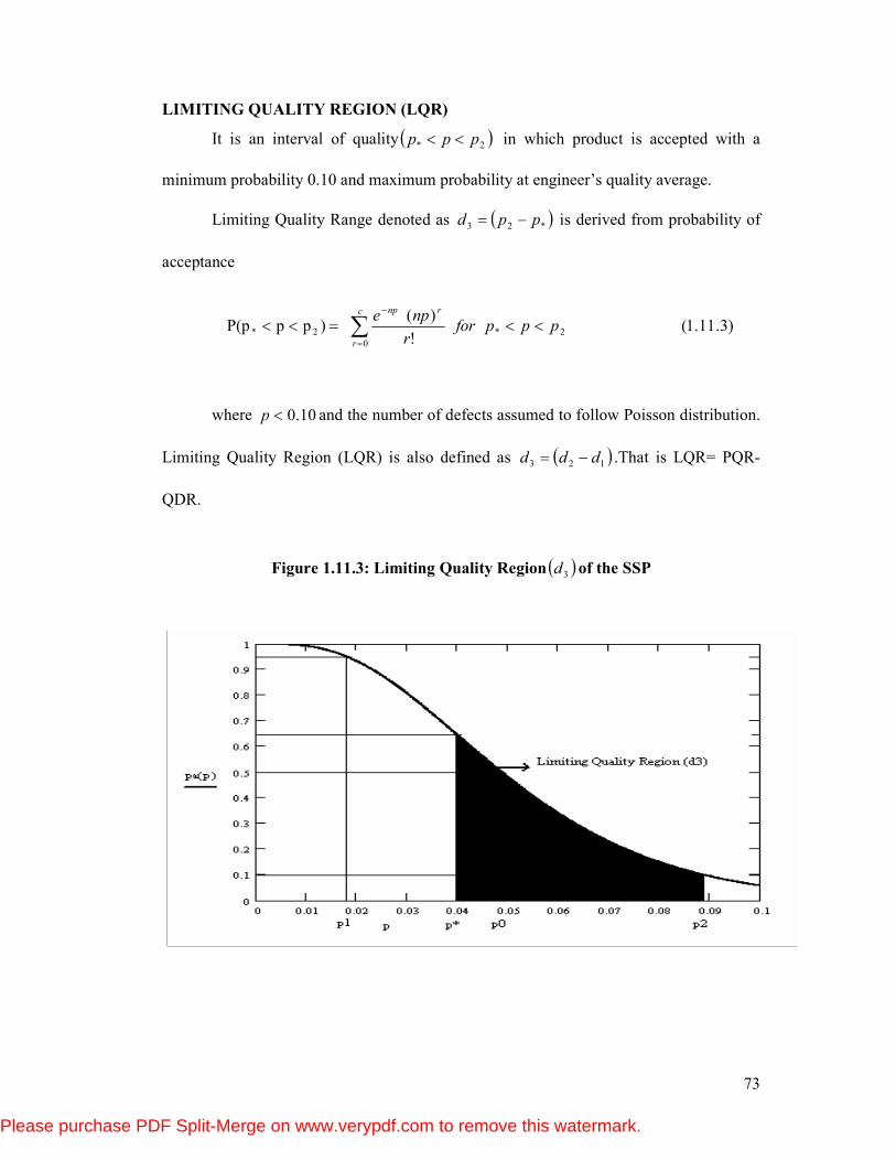
73

LIMITING QUALITY REGION (LQR)

It is an interval of quality ( )2* ppp << in which product is accepted with a

minimum probability 0.10 and maximum probability at engineer’s quality average.

Limiting Quality Range denoted as ( )*23 ppd −= is derived from probability of

acceptance

where 10.0<p and the number of defects assumed to follow Poisson distribution.

Limiting Quality Region (LQR) is also defined as ( )123 ddd −= .That is LQR= PQR-

QDR.

Figure 1.11.3: Limiting Quality Region ( )3d of the SSP

)3.11.1(!

)( )ppP(p 2*

0

2* pppforr

npec

r

rnp

<<=<< ∑=

−


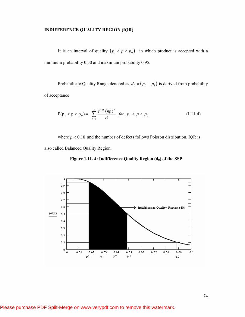
74

INDIFFERENCE QUALITY REGION (IQR)

It is an interval of quality ( )01 ppp << in which product is accepted with a

minimum probability 0.50 and maximum probability 0.95.

Probabilistic Quality Range denoted as ( )100 ppd −= is derived from probability

of acceptance

where 10.0<p and the number of defects follows Poisson distribution. IQR is

also called Balanced Quality Region.

Figure 1.11. 4: Indifference Quality Region (d0) of the SSP

)4.11.1(!

)( )ppP(p 01

0

01 pppforr

npec

r

rnp

<<=<< ∑=

−


75

SECTION1.12: TIGHTENED- NORMAL- TIGHTENED (TNT) SAMPLING SCHEMES

This section deals with a brief review on the selection of Tightened- Normal-

Tightened (TNT) schemes. The schemes considered here are of Type TNT (n1, n2, 0) and

TNT(n, c1, c2).

TNT sampling inspection is a scheme involving switching between two sampling

plans namely Normal and Tightened plan which was proposed by Calvin (1977). MIL-

STD-105D (1963) contains a scheme with fixed sample size and two different acceptance

criteria. A single sampling plan with zero acceptance number and small sample size is

often employed in situations involving costly or destructive testing by attributes. The

smaller sample size is warranted due to the costly nature of testing and zero acceptance

number arises out of desire to maintain a steep OC curve. Calvin (1977) suggests that the

switching between two sample sizes with zero acceptance number creates an inflection

point on the OC curve, which results in an improved probability of acceptance at good

quality where the smaller sample size dominates. Suresh (1993) has studied TNT of both

type namely, TNT (n, n2; 0) and TNT (n,0,1).

The conditions for application of TNT schemes are:

a) Production is in a steady state, so that results of past, present and future lots

are broadly indicative of a continuing process.

b) Lots are submitted substantially in the order of their production.

c) Inspection is by attributes, with quality defined as the fraction non-conforming ‘p’.

The Operating Procedure for a TNT scheme of type TNT(n1, n2; 0) Scheme is as

follows:

Step 1:

Inspect under tightened inspection using a single sampling plan with the larger

sample size n1 and acceptance number c=0. If ‘t’ lots in a row are accepted under

tightened inspections then switch to normal inspection (Step2).


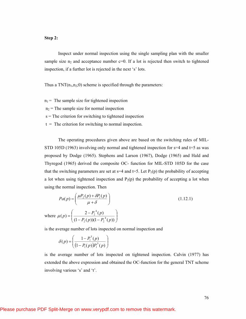
76

Step 2:

Inspect under normal inspection using the single sampling plan with the smaller

sample size n2 and acceptance number c=0. If a lot is rejected then switch to tightened

inspection, if a further lot is rejected in the next ‘s’ lots.

Thus a TNT(n1,n2;0) scheme is specified through the parameters:

n1 = The sample size for tightened inspection

n2 = The sample size for normal inspection

s = The criterion for switching to tightened inspection

t = The criterion for switching to normal inspection.

The operating procedures given above are based on the switching rules of MIL-

STD 105D (1963) involving only normal and tightened inspection for s=4 and t=5 as was

proposed by Dodge (1965). Stephens and Larson (1967), Dodge (1965) and Hald and

Thyregod (1965) derived the composite OC- function for MIL-STD 105D for the case

that the switching parameters are set at s=4 and t=5. Let P1(p) the probability of accepting

a lot when using tightened inspection and P2(p) the probability of accepting a lot when

using the normal inspection. Then

+

+=

δµδµ )()(

)( 12 pPpPpPa (1.12.1)

where

−−

−=

))(1))((1(

)(2)(

4

22

4

2

pPpP

pPpµ

is the average number of lots inspected on normal inspection and

( )

−

−=

)()(1

)(1)(

5

11

5

1

pPpP

pPpδ

is the average number of lots inspected on tightened inspection. Calvin (1977) has

extended the above expression and obtained the OC-function for the general TNT scheme

involving various ‘s’ and ‘t’.


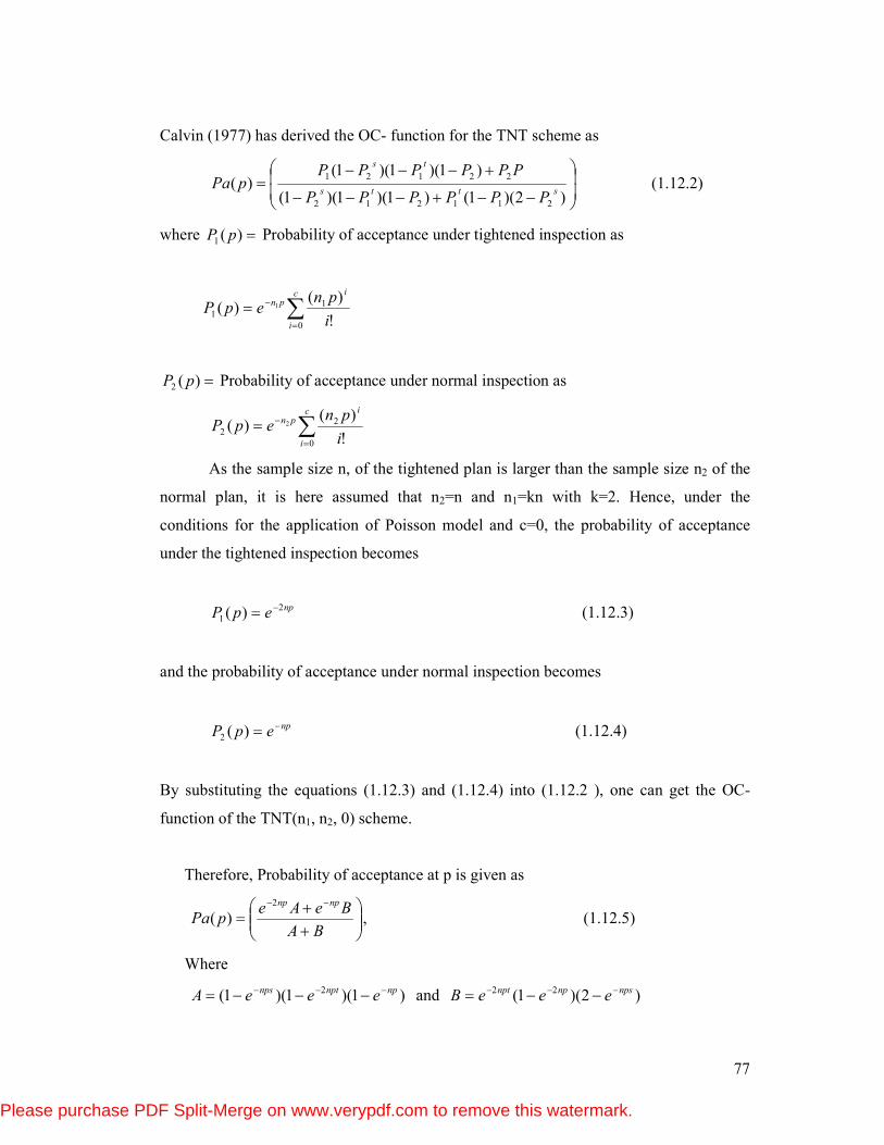
77

Calvin (1977) has derived the OC- function for the TNT scheme as

−−+−−−

+−−−=

)2)(1()1)(1)(1(

)1)(1)(1()(

211212

22121

stts

ts

PPPPPP

PPPPPPpPa (1.12.2)

where =)(1 pP Probability of acceptance under tightened inspection as

∑=

−=c

i

ipn

i

pnepP

0

11

!

)()( 1

=)(2 pP Probability of acceptance under normal inspection as

∑=

−=c

i

ipn

i

pnepP

0

22

!

)()( 2

As the sample size n, of the tightened plan is larger than the sample size n2 of the

normal plan, it is here assumed that n2=n and n1=kn with k=2. Hence, under the

conditions for the application of Poisson model and c=0, the probability of acceptance

under the tightened inspection becomes

npepP 2

1 )( −= (1.12.3)

and the probability of acceptance under normal inspection becomes

npepP −=)(2 (1.12.4)

By substituting the equations (1.12.3) and (1.12.4) into (1.12.2 ), one can get the OC-

function of the TNT(n1, n2, 0) scheme.

Therefore, Probability of acceptance at p is given as

++

=−−

BA

BeAepPa

npnp2

)( , (1.12.5)

Where

)1)(1)(1(2 npnptnps

eeeA−−− −−−= and )2)(1(

22 npsnpnpteeeB

−−− −−=


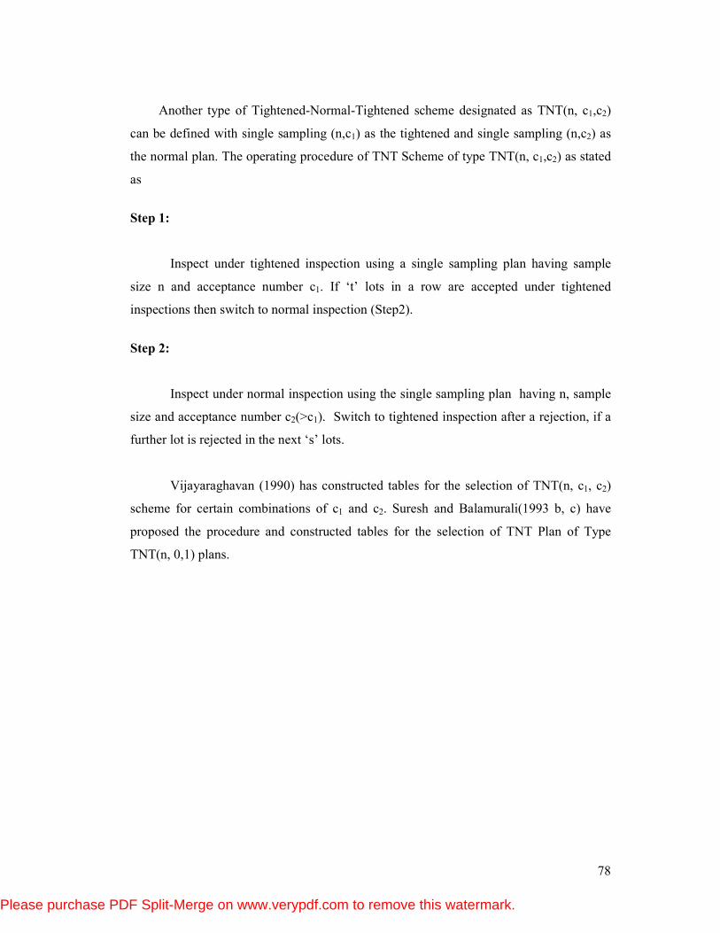
78

Another type of Tightened-Normal-Tightened scheme designated as TNT(n, c1,c2)

can be defined with single sampling (n,c1) as the tightened and single sampling (n,c2) as

the normal plan. The operating procedure of TNT Scheme of type TNT(n, c1,c2) as stated

as

Step 1:

Inspect under tightened inspection using a single sampling plan having sample

size n and acceptance number c1. If ‘t’ lots in a row are accepted under tightened

inspections then switch to normal inspection (Step2).

Step 2:

Inspect under normal inspection using the single sampling plan having n, sample

size and acceptance number c2(>c1). Switch to tightened inspection after a rejection, if a

further lot is rejected in the next ‘s’ lots.

Vijayaraghavan (1990) has constructed tables for the selection of TNT(n, c1, c2)

scheme for certain combinations of c1 and c2. Suresh and Balamurali(1993 b, c) have

proposed the procedure and constructed tables for the selection of TNT Plan of Type

TNT(n, 0,1) plans.


Documents

CHAPTER I INTRODUCTION - Shodhgangashodhganga.inflibnet.ac.in/bitstream/10603/33882/1/... · 2018-07-02 · 1 CHAPTER I INTRODUCTION In this chapter concept, terminologies and symbols