CHAPTER- I PRELIMINARIES

1.1 Introduction

1.2 Fixed Point Property

1.3 Common Fixed Point

1.4 Banach Contraction Principle

1.5 Weak Conditions of Commutat ivi ty for

Single-Valued Mappings

1.6 Weak Conditions of Commutat ivi ty for

Hybrid Mappings

1.7 2-Metric Spaces

PRELIMINARIES

1.1 INTRODUCTION

LetXbeset. We consider a mapping T: X ->X. An elements e^fissaid

to be a fixed point of the mapping Tif Tx = x. By a fixed point theorem

we shall understand a statement which asserts that under certain

conditions (on the mapping T and on the space X) a mapping T of X

admits one or more fixed points.

Fixed point theory plays very important role in areas like non­

linear analysis and non-linear operators which are relatively young but

fully developed areas for research. There are several domains like

classical analysis, functional analysis, operator theory, topology,

algebraic toplogy, etc. where the study of existence of fixed points falls.

The important applications of this theory are in areas like non-linear

oscillations, fluid flow, approximation theory, chemical reactions,

steady state temperature distribution, economic theories and initial and

boundary value problems for ordinary, partial differential and integral

equations. For details one can see Martin [82], Smart [116], Collatz

[25], Moore [83], Kreyszig [73], Cronion [26] Cesari [15], Leggett and

Williams [77] etc.

- : l :-

Perhaps Brouwer's [11] was the first to give the proof of a fixed

point theorem which states that a continuous self-mapping of a closed

unit ball in n-dimensional Euclidean space has atleast one fixed point.

We can find several proofs of this basic result in existing literature.

Mathematicians used several tools from different areas to prove

Brouwer's fixed point theorem like Alexendroff and Hopf [3] used

Algebraic topological techniques while Birkhoff and Kellogg [9] used

classical analysis to prove it.

Such theorems, where these spaces i.e. subsets of R", are not of

much use in functional analysis where one is generally concerned with

infinite dimensional subsets of some function space. In view of this,

attempts were made in this direction and the first infinite dimensional

fixed point theorem was proved by Birkhoff and Kellogg [9] in 1922.

Subsequently Schauder [102] extended Brouwer's theorem to the

compact convex subsets of a normed linear space. This theorem was

further extended to locally convex topological vector space by Tychonoff

[119]. Later on, Banach [8] obtained the fixed point theorem for

contraction mappings which is very famous because its proof is simple

and does not require much topological background.

-: 2 :-

In recent years Kannan ([60], [61]). Husain and Sehgal [47]

Caristi [14] etc. have considered several generalizations of contraction

mappings and proved a multitude of results.

Various notions have been included in different sections of this

chapter which are essential for presentation of results in the subsequent

chapters. For a detailed study of fixed point theory one can refer to the

books of Istratescu [53], Rus [101] and Smart [116]. Three survey

papers by Rhoades ([96], [98], [99]) are also of special significance for

the comparative study of various contractive conditions scattered in the

literature.

1.2 FIXED POINT PROPERTY

LetAfbe a topological space. We define a mapping 7fromA'into

itself. If for every continuous mapping T from A" into itself there exists

a point x e X such that Tx = x, then we say that the topological space A*

has a fixed point property. This property is a toplogical property. A set

with fixed point property is expected to be compact and contractible.

Any set without one of these properties will certainly have a mapping

with no fixed point. Real line and circl e are examples which do not have

the fixed point property. We can refer to Smart [116] for more details.

-: 3 :-

However, a counter example was given by Kinoshita [70] whereby he

proved that these conditions are neither necessary nor sufficient for-a

space to have the fixed point property.

13 COMMON FIXED POINT

In the subsequent chapters we study common fixed points of a

pair of mappings, both single-valued and multivalued and of a family of

mappings. Let Xbe an arbitrary set and let 3 be a family of mappings

T: X-> X. A point z e Xis called a common fixed points for the family

if T(z) = z for all T e 3 . The first result for family of mappings was

proved by Markov in 1936. Kakutani gave a direct proof of Markov's

theorem in 1938 and also proved a fixed point theorem for groups of

affine mappings. Ryll-Nardzewski obtained an important extension of

the results of Markov and Kakutani in 1966. Day [27] also proved a

more general theorem. For further work in this direction one can refer

to Greanleaf [42], Huff [46] and many others.

1.4 BANACH CONTRACTION PRINCIPLE

It was S. Banach who after Brouwer's in 1922 gave the fundamental

result which is popularly known as Banach contraction principle or

contraction mapping theorem. In fact this is the most celebrated result

- : 4 :-

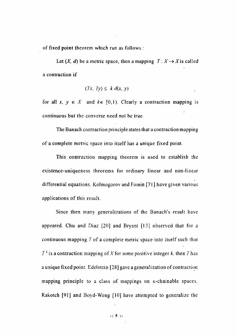
of fixed point theorem which run as follows :

Let (X, d) be a metric space, then a mapping T: X -> Xis called

a contraction if

(Tx, Ty) < k d(x, y)

for all x, y e X and ke [0,1). Clearly a contraction mapping is

continuous but the converse need not be true.

The Banach contraction principle states that a contraction mapping

of a complete metric space into itself has a unique fixed point.

This contraction mapping theorem is used to establish the

existence-uniqueness theorems for ordinary linear and non-linear

differential equations. Kolmogorov and Fomin [71 ] have given various

applications of this result.

Since then many generalizations of the Banach's result have

appeared. Chu and Diaz [20] and Bryant [13] observed that for a

continuous mapping T of a complete metric space into itself such that

T Ms a contraction mapping of X for some positive integer k, then Thas

a unique fixed point. Edelstein [28] gave a generalization of contraction

mapping principle to a class of mappings on s-chainable spaces.

Rakotch [91] and Boyd-Wong [10] have attempted to generalize the

-: 5 :-

Banach's result by replacing the lipschitz constant k by some real

valued functions whose values lie in [0, 1). Various attempts were made

to replace the contractive condition by some more general mapping

condition in order to accomodate a variety of continuous and

discontinuous functions. Recently, Rhoades ([96], [98], [99]) made a

systematic study and compared the various contractive conditions

scattered in the literature. Though it is not possible to mention all the

contractive definitions, yet we do mention just a few which are relevant

to the contents of the present work.

(1) Hardy and Rogers [45]

d(Tx, Ty) < a[d(x, Tx) + d(y, Ty)]+b[d(y, Tx)+ d(x. Ty)]

+ c d{x, y)

for all x, y e X, a, b, c > 0, 2a + 2*i + c < ]

(2) Ciric [21]

d(Tx, Ty) < a max {d(x, y) . d{x, Ty). d(y, Tx). d{\\ Ty),

d(x, Tx)}

for all x, y e X and a e [0, 1).

(3) Boyd and Wong [10]

d(Tx, Ty) < </>[d(x,y)]

-: 6 :-

for all x, y e Xand </>: R' -» R~ is upper semicontinuous where $ 0 < /

for each / > 0.

(4) Fisher [31] b[d(x, Ty)]2 + c[d(Sx, y)}2

d{Sx, Ty) < d(x, Ty) + d(Sx, y)

\id{x, Ty) + d{Sx, y) * 0, 0 < b, c, b + c < 1

or d(Sx, Ty) = 0, if d(x, Ty) + d(Sx, y) = 0.

1.5 WEAK CONDITIONS OF COMMUTATIVITY FOR

SINGLE-VALUED MAPPINGS

In an attempt to generalize the notion of commutativity for

single-valued mappings, Sessa [103] introduced the idea of weak

commutativity which can be stated as follows.

Definition 1.5.1 Let S and /be mappings of a metric space (X, aOinto

itself. The pair {S, 1} is said to be weakly commuting if

d(ISx, Six) < d(Sx, Ix) VA- e X.

Obviously a commuting pair is always weakly commuting but the

converse is not generally true.

Example 1.5.2 Consider the setA^ [0,1] with the usual metric. Let

Ix = x/2 and Sx = x/(2-*-x) for every x e X.

-: 7 :-

X X

Then for all xeX, ISx = , Six = ; obviously 5 and / 4+2x 4+A

are not commuting. Further

X X X2

d(ISx, Six) = | | = 4+2* 4+A- (4+A-) (4+2JC)

X2 X X

< = = d(Sx, Ix) 4+2* 2 2+x

so, S and I are weakly commuting.

Subsequently. Jungck [56] observed that if Ix = x3 and Sx = 2x}

then I and S are not of weakly commuting. Thus he made an extension

of the concept weak commutativity by introducing a new concept of

compatible mappings.

Definition 1.5.3 Two self mappings S and I of a metric space (X, d)

are compatible iff Jim d{SIxn, ISxn) = 0 , whenever [xn\ is a /7-»0O

sequence in X such that Urn Sx = Hm Ix = t for some / e X.

Clearly, any weakly commuting pair is compatible but the converse

need not be true as shown in the following example.

Example 1.5.4 Let Ix = x' and Sx = 2-x with X = R. \ /(xn)-S(xt)\ -

\x -7 | I x2 +x + 2 I ->0 iff A- ->1 and I JS(x ) - SI(x ) I =6 I x -11-—>0

if x„->l. Thus S and / are compatible but are not weakly commuting

pair; e.g. let A' = 0.

-: 8 :-

Later on Jungck et. al. [57] introduced the concept of (^)type

compatible mappings which is stated as follows.

Definition 1.5.5 Let S and J be mappings from a metric space (X, d)

into itself. The pair [S, 1} is said to be (A)type compatible on Xif when­

ever {xj is a sequence inXsuch that lim Sxn= lim Ixn = z in X, then n—>oo n—»oo

d(SIxn, Uxn) ->0 and d(ISxn, SSxn)-+0, as n->oo .

It is shown in Jungck et. al. [57] that under certain conditions the

compatible and (A)type compatible mappings are equivalent, where-as

in ([57], [40]) it is demonstrated by suitable examples that if S and / are

discontinuous then the two concepts are independent of each other. The

following examples also support this observation.

Example 1.5.6 Let X= R with the usual metric. We define S, I : X

- » X a s follows

r i/x-\ x*o ( I/A-1 , A-*O Sx = \ and Ix = \

K 0 , x=0 0 , -v=0 '

Both S and / are discontinuous at x = 0 and for any sequence {A/;J in X.

we have d(SIxn, ISxJ = 0. Hence the pair {S , I) is compatible. Now

consider the sequence A' = n e N. The Sx -> 0 and 7A- ->0 as n-*<x> and

d(SIxii, IIxJ = | w - «9 | ->oo, as w->oo.

-: 9 :-

Example 1.5.7 Now we define l/x\ x>\ ( - 1 A \ x>l

1 , 0<x<\ andlx= i 1 , 0<x<l 0 , x<0 0 , *<0

Observe that the restriction S and / on (-<», 1 ] are equal, thus we

take a sequence {xj in (1, oo). Then {SxJ c (0, 1) and {IxJ c (-1, 0).

Thus for every «, IIx = 0, JSx = 1, Six = 0, SSx = 1 so that

£/(5/xfl, //xn) = 0, ^(75^ SSx) = 0 for every n e N. This show that the

pair {S, 1} is 04)type compatible. Now let xn = n, n e N. Then /A„-> 0,

Sx -^0 as «->oo and Six = 0, AS* = 1 for every n e N and so

d(SIxn, ISxJ * 0 as «-»oo . Hence the pair {S,I\ is not compatible.

Recently, in [90], Pathak et. al. introduced yet another class of

mappings called (P)type compatible mappings and compared with the

compatible and compatible mappings of type {A) which is stated as.

Definition 1.5.8 Let S, I: (X, d)-^(X, d) be mappings. S and I are said

to be compatible of type (P) if

Urn d(SSx , IIx ) = 0 M-»0O

whenever {x\ is a sequence in X such that

Urn Sx = Um lx = z for some r in X. n n

n—>oo H—»oo

The following propositions show that the definitions 1.5.3. 1.5.5

-: 10 :-

Sx= {

and 1.5.8 are equivalent under some conditions.

Proposition 1.5.9 Let S, I: (X,d) -±(X, d) be continuous mappings. If

5 and 1 are compatible, then they are compatible of type {A).

Proposition 1.5.10 Let S, I: (X,d) ->(X, d) be compatible mappings of

type (A) if one of S and / is continuous, then S and / are compatible.

Proposition 1.5.11 Let S, I: (X,d) -+{X, d) be continuous mappings.

Then S and / are compatible if and only if they are compatible

of type (A).

Proposition 1.5.12 Let S, I: (X,d) -+(X, d) be continuous mappings.

Then S and / are compatible if and only if they are compatible

of type (P).

Proposition 1.5.13 Let S, I: (X,d) ->(X, d) be compatible mappings of

type (A). If one of S and / i s continuous, then S and/ are compatible of

type (P).

Proposition 1.5.14 Let S, I: (X,d) -+Qi,d) be continuous mappings. Then

(i) S and / are compatible if and only if they are compatible of type (P).

(ii) S and / are compatible of type {A) if and only if they are

compatible of type (P).

-: 11 :-

Next, we give several properties of compatible mappings of type

(A) and type (P).

Proposition 1.5.15 Let S, I: (X,d) -+(X, d) be mappings. If S and / are

compatible of type (A) and Sz = Iz for some z e X. then Slz =

SSz = JIz = ISz.

Proposition 1.5.16 Let S, I: {X,d) ->(X d) be mappings. If S and / are

compatible of type (P) and Sz = Iz for some z e X. then Slz =

S&r = llz = /&.

Proposition 1.5.17 Let S, I: (X </) ->(X, ^) be compatible mappings of

type (A) and let Sxn, Ixr -» f as «-»<x> for some / e X Then the following

holds: (i) Jim Six = It, if / is continuous at f„

W->00

(ii) /r'/w /5!xn = 57, if S is continuous at 7. n-»oo

(iii) 57* = 757 and St = It, if S and / are continuous at t.

Proposition 1.5.18 Let S, J: {X, d) ->(X, d) be compatible mappings of

type (P) and let Sxn, Txn -» t as w-»oo for some / e X. Then the following

holds: (i) lim IIxn = St, if S is continuous at /,

w->oo

(ii) Jim SSxn = It. if / is continuous at t, n->ao

(iii) S7f = ISt and St = 7/, if S and / are continuous at /.

- : 12 :-

1.6 WEAK CONDITIONS OF COMMHTATIVITY FOR HYBRID MAPPINGS

Motivated from Sessa [103] and Jungck [56], the concepts of

weak commutativity and compatibility for nonself hybrid mappings

were given by Hadzic-Gajic [43] and Hadzic [44] which runs as

follows.

Definition 1.6.1 Let A'be anon-empty subset of a metric space (X, d).

F : K ->2A" and T : K ->X. Then the pair {F, T} is said to be weakly

commuting if for every x, y in K such that x e Fy and Ty e K,

d(Tx, FTy) < d(Ty, Fy).

Definition 1.6.2 Let K be a non-empty subset of a metric space-(A', d),

F : K ->2X and T : K ->X. Then the pair \F, T) is said to be

compatible if for e\ery sequence {xj form K and from the relation

Jim d(Fx , Tx ) = 0 and Tx e K, it follows that n—>oo

Jim d{Tyn, FTxJ = 0

for every sequence {yj from K such that>>w e Fxn.

For K = X and F single-valued, the definitions 1.6.1 and 1.6.2

reduce to definitions 1.5.1 and 1.5.3 respectively. It is well known that

weakly commuting pair {F, T) is compatible but the converse is not

-: 13 :-

necessarily true as shown in Example 1.5.4.

For a pair of hybrid self-mapping of X, Kaneko-Sessa [59]

extended the notion of weak commutativity and compatibility which we

give in the following.

Definition 1.6.3 Let (X, d) be a metric space, F: X -> 2X and T: X -> X.

The pair (F, T) is called weakly commuting if for each x e X,

TFx e 2s and

H(FTx, TFx) < d(Tx , FA),

where H is the Hausdorff metric defined on 2X induced by d.

Definition 1.6.4 Two mappingsF:X^>2Xand T:X-^Xare compatible

if and only if

TFxe 2X for all x eX and H(FTxn, TFx J ->0

whenever {xj is a sequence in X such that Fxn —> M e 2A and

Tx ->• / e M. where H is the Hausdorff metric defined on 2X. n

Khan et. al. [69] and Singh et. al. [114] have used the following

weak conditions of commutativity.

Definition 1.6.5 The mappings F: X -> 2X and T : X -» X are called

quasi commuting at * e Xif TFx c F7x. the pair {F, T) is said to be

quasi-commute on X if it is quasi-commute at every x e X.

- : 14 :-

Singh et. al. [114] used the term commutativity for the same

which is somewhat misleading as it is a condition weaker than

commutativity.

Definition 1.6.6 The mappings F : X -» 2V and T : X -> X are-called

weakly commuting at x e X, if

H(TFx , FTx) < d(Tx, Fx).

T and Fare weakly commuting on X, if they commute weakly at

every x e X. For F single-valued, this definition reduces to

definition 1.5.1.

1.7 2-METRIC SPACES

Following Gahler [37] and White [121] we have the following

definitions :

Definition 1.7.1 Let X be a nonempty set. (X, d) is called a 2-metric

space, if d is a mapping from Xx X x J - > [0,oo) satisfying the following

conditions :

(i) For any a, b eX, a± b. there exists a point c e Jf such that

d(a, b, c) * 0,

(ii) d(a, b, c) = 0, if at least two of three points a, b, c are equal.

(iii) d(a, b, c) = d(b, c, a) = d(a, c, b),

(iv) d(a, b, c) < d(a, b, d)+d(a, d, c)+d(d, b, c) Va.b.ceX.

-: 15 :-

It has been shown by Gahler [37] that the 2-metric of d is non-

negative and although d is a continuous function of any one of its three

arguments, it need not be continuous in two arguments. A 2-metric d

which is continuous in all of its arguments will be called continuous. We

further mention that a 2-metric abstracts the properties of the area

function for Euclidean triangles in just the same manner as a metric

abstracts the properties of the length function. We shall therefore, call

property (iv) as triangular area inequality.

Definition 1.7.2 A sequence {xj in a 2-metric space (X, d) is said to

be convergent to a point z in X, denoted by Jim xn = z or xn —> z as w->oo. n—>oo

if Jim d(xn, z, a) = 0 for all a in X. The point z is called the limit of rt-»oo

the sequence {xj inX.

Definition 1.7.3 A sequence {x } in a 2-metric space (X, d) is said to

be Cauchy sequence if Jim d(xm , xn, a) = 0 for all a e X.

Definition 1.7.4 A 2-metric space (X, d) is said to be complete if

every Cauchy sequence \nX\s convergent.

Note that, in a 2-metric space (X, d), a convergent sequence need

not be a Cauchy sequence, but every convergent sequence is a Cauchy

sequence when the 2-metric d is continous on X ([85]).

-: 16 :-

Definition 1.7.5 A mapping S from a 2-metric space {X, d) into itself is

said to be sequentially continuous atz e ^fif for every sequence {xj in

X such that Urn d{xn, x, a) = 0 for all a e X, implies hm (Sxn,Sz,a)=0 n->oo n-»oo

It is well known that a 2-metric dis always sequentially continuous

in two variables thus it will also be sequentially continuous in all the

three variables. In this case ^is said to be continuous.

-: 17 :-