Chapter Five

Average Permeability

The most difficult reservoir properties to determine usually are the level and

distribution of the absolute permeability throughout the reservoir. They are more

variable than porosity and more difficult to measure. Yet an adequate knowledge of

permeability distribution is critical to the prediction of reservoir depletion by any

recovery process. It is rare to encounter a homogeneous reservoir in actual practice. In

many cases, the reservoir contains distinct layers, blocks, or concentric rings of

varying permeabilities. Also, because smaller-scale heterogeneities always exist, core

permeabilities must be averaged to represent the flow characteristics of the entire

reservoir or individual reservoir layers (units). The proper way of averaging the

permeability data depends on how permeabilities were distributed as the rock was

deposited. There are three simple permeability-averaging techniques that are

commonly used to determine an appropriate average permeability to represent an

equivalent homogeneous system. These are:

• Weighted-average permeability

• Harmonic-average permeability

• Geometric-average permeability

Weighted-Average Permeability

This averaging method is used to determine the average permeability of layered-

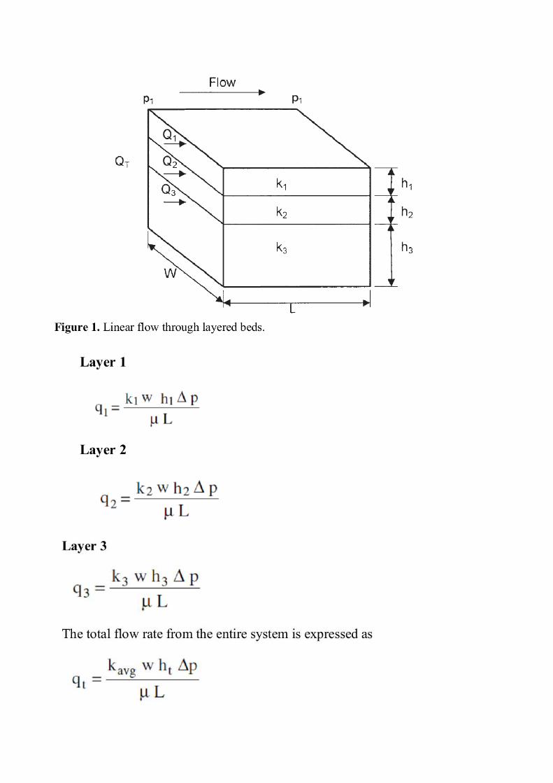
parallel beds with different permeabilities. Consider the case where the flow system is

comprised of three parallel layers that are separated from one another by thin

impermeable barriers, i.e., no cross-flow, as shown in Figure 1. All the layers have the

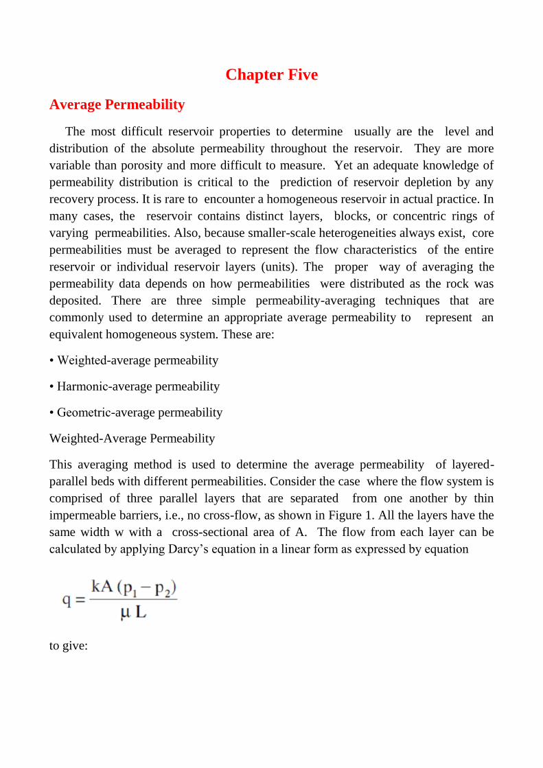
same width w with a cross-sectional area of A. The flow from each layer can be

calculated by applying Darcy’s equation in a linear form as expressed by equation

to give:

Where qt=total flow rate

kavg=average permeability for entire model

w= width of the formation

∆p= p1 - p2

ht= total flow rate

The total flow rate qt is equal to the sum of the flow rates through each layer or:

Combining the above expressions gives:

The average absolute permeability for a parallel-layered system can be expressed in

the following form:

The above equation is commonly used to determine the average permeability of a

reservoir from core analysis data.

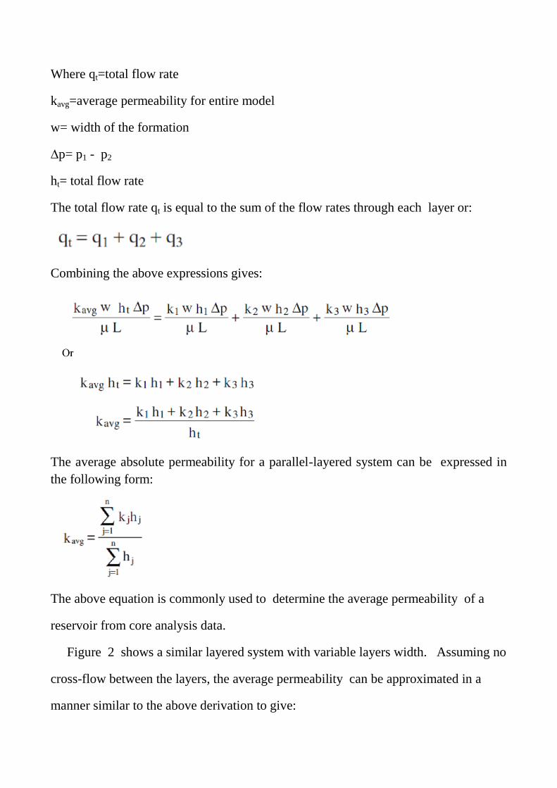
Figure 2 shows a similar layered system with variable layers width. Assuming no

cross-flow between the layers, the average permeability can be approximated in a

manner similar to the above derivation to give:

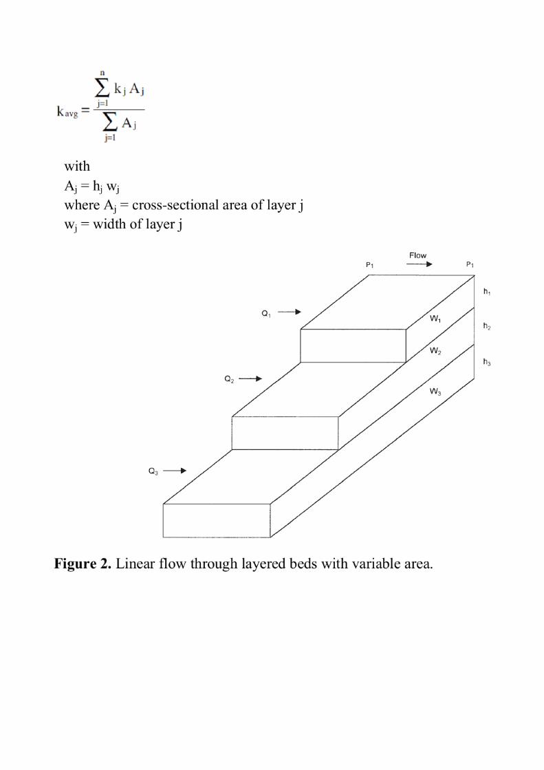
Radial flow

This case is similar to linear layers except for the circular geometry of the porous

medium. All layers have radius re and are penetrated by a well of radius rw as

depicted in Fig. 3. The common inlet and outlet pressures are Pe and Pw,

respectively. For each layer, Darcy's equation is written as:

and the total flow rate is

Employing an average permeability, k, Darcy's equation for the whole medium will be

Comparing the above equations yields

Harmonic-Average Permeability

Permeability variations can occur laterally in a reservoir as well as in the vicinity of

a well bore. Consider Figure 4, which shows an illustration of fluid flow through a

series combination of beds with different permeabilities.

For a steady-state flow, the flow rate is constant and the total pressure drop Δp is equal

to the sum of the pressure drops across each bed, or

Substituting for the pressure drop by applying Darcy’s equation, i.e., Darcy's

Equation, gives:

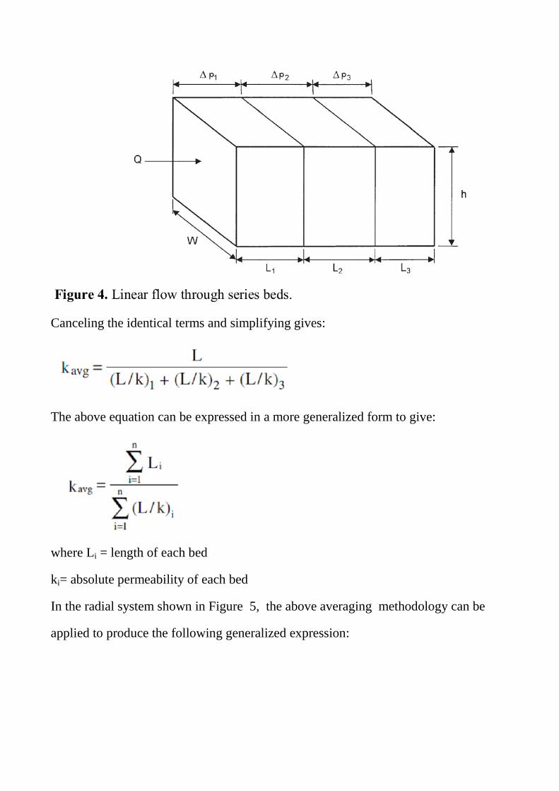
Canceling the identical terms and simplifying gives:

The above equation can be expressed in a more generalized form to give:

where Li = length of each bed

ki= absolute permeability of each bed

In the radial system shown in Figure 5, the above averaging methodology can be

applied to produce the following generalized expression:

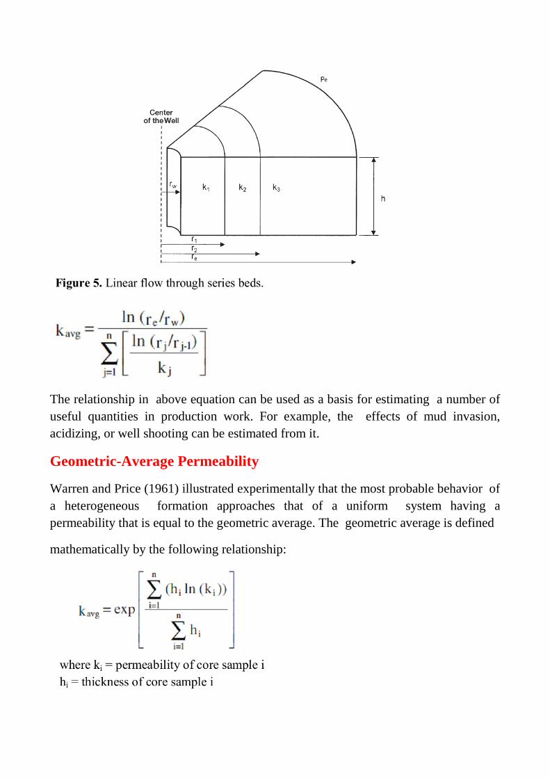
The relationship in above equation can be used as a basis for estimating a number of

useful quantities in production work. For example, the effects of mud invasion,

acidizing, or well shooting can be estimated from it.

Geometric-Average Permeability

Warren and Price (1961) illustrated experimentally that the most probable behavior of

a heterogeneous formation approaches that of a uniform system having a

permeability that is equal to the geometric average. The geometric average is defined

mathematically by the following relationship:

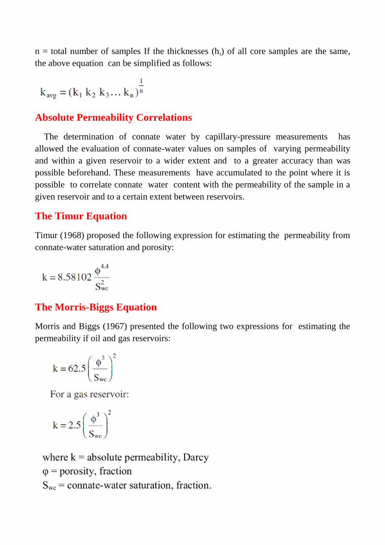
n = total number of samples If the thicknesses (hi) of all core samples are the same,

the above equation can be simplified as follows:

Absolute Permeability Correlations

The determination of connate water by capillary-pressure measurements has

allowed the evaluation of connate-water values on samples of varying permeability

and within a given reservoir to a wider extent and to a greater accuracy than was

possible beforehand. These measurements have accumulated to the point where it is

possible to correlate connate water content with the permeability of the sample in a

given reservoir and to a certain extent between reservoirs.

The Timur Equation

Timur (1968) proposed the following expression for estimating the permeability from

connate-water saturation and porosity:

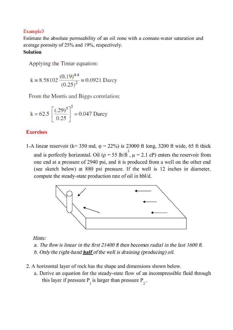
The Morris-Biggs Equation

Morris and Biggs (1967) presented the following two expressions for estimating the

permeability if oil and gas reservoirs:

Examples

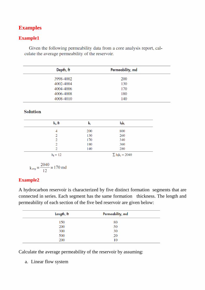
Example1

Example2

A hydrocarbon reservoir is characterized by five distinct formation segments that are

connected in series. Each segment has the same formation thickness. The length and

permeability of each section of the five bed reservoir are given below:

Calculate the average permeability of the reservoir by assuming:

a. Linear flow system

b. Radial flow system

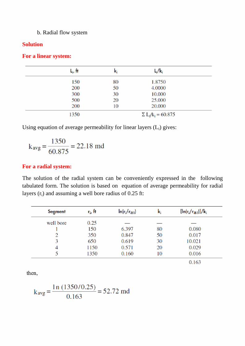
Solution

For a linear system:

Using equation of average permeability for linear layers (Li) gives:

For a radial system:

The solution of the radial system can be conveniently expressed in the following

tabulated form. The solution is based on equation of average permeability for radial

layers (ri) and assuming a well bore radius of 0.25 ft:

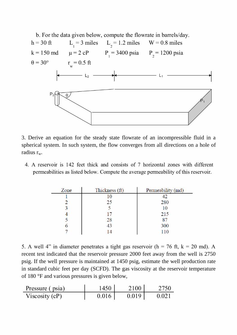
3. Derive an equation for the steady state flowrate of an incompressible fluid in a

spherical system. In such system, the flow converges from all directions on a hole of

radius rw.

5. A well 4” in diameter penetrates a tight gas reservoir (h = 76 ft, k = 20 md). A

recent test indicated that the reservoir pressure 2000 feet away from the well is 2750

psig. If the well pressure is maintained at 1450 psig, estimate the well production rate

in standard cubic feet per day (SCFD). The gas viscosity at the reservoir temperature

of 180 °F and various pressures is given below,

6. Because of low permeability, the well of Exercise 5 was acidized. This stimulation

process increased the rock permeability to 95 md in a zone only 5 feet in diameter

around the well.

a. Estimate the reservoir's average permeability after acidizing.

b. Estimate the well production rate after acidizing

c. How much increase (or decrease) in the well’s production do we gain with

acidizing?

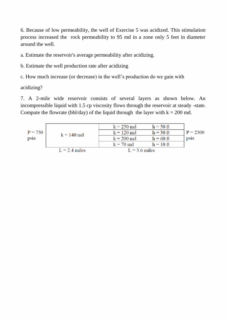
7. A 2-mile wide reservoir consists of several layers as shown below. An

incompressible liquid with 1.5 cp viscosity flows through the reservoir at steady -state.

Compute the flowrate (bbl/day) of the liquid through the layer with k = 200 md.