Embed Size (px)
Citation preview
Chapter 12
Inferences for Proportions
Lesson 12-1
Inference for a Population
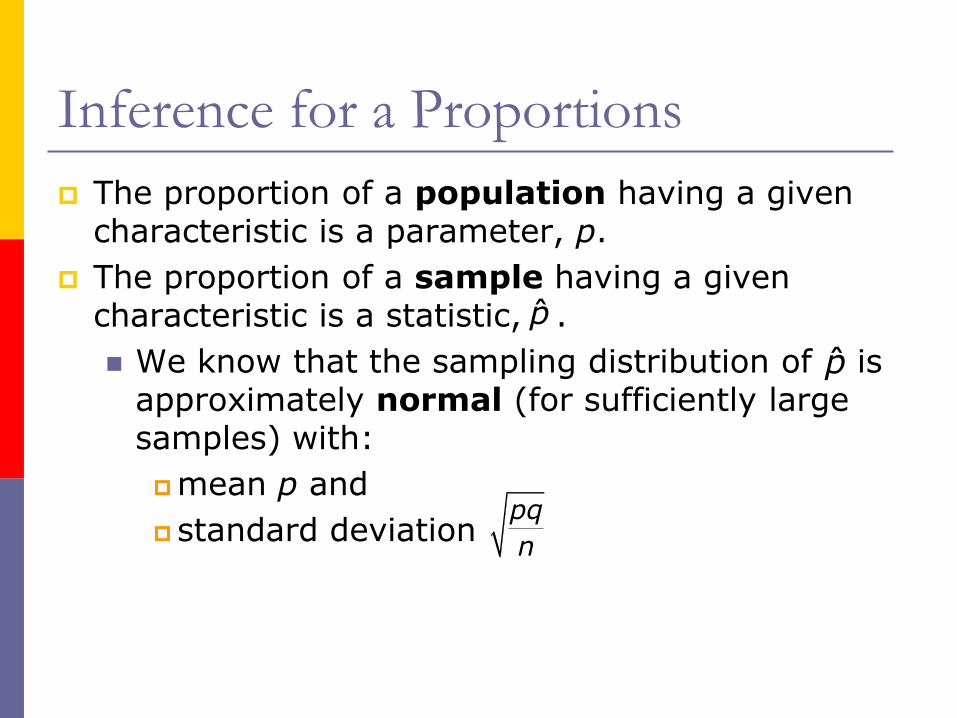
Inference for a Proportions
The proportion of a population having a given characteristic is a parameter, p.
The proportion of a sample having a given characteristic is a statistic, .
We know that the sampling distribution of is approximately normal (for sufficiently large samples) with:
mean p and
standard deviation
p̂
p̂
pq
n
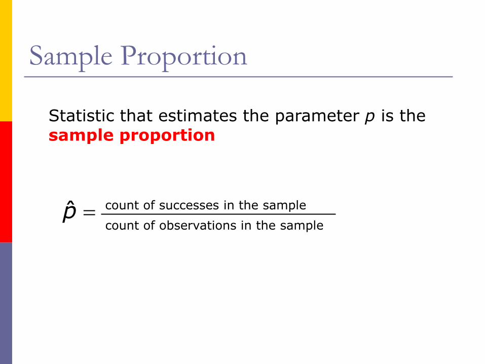
Sample Proportion
Statistic that estimates the parameter p is the sample proportion
p̂ count of successes in the sample
count of observations in the sample
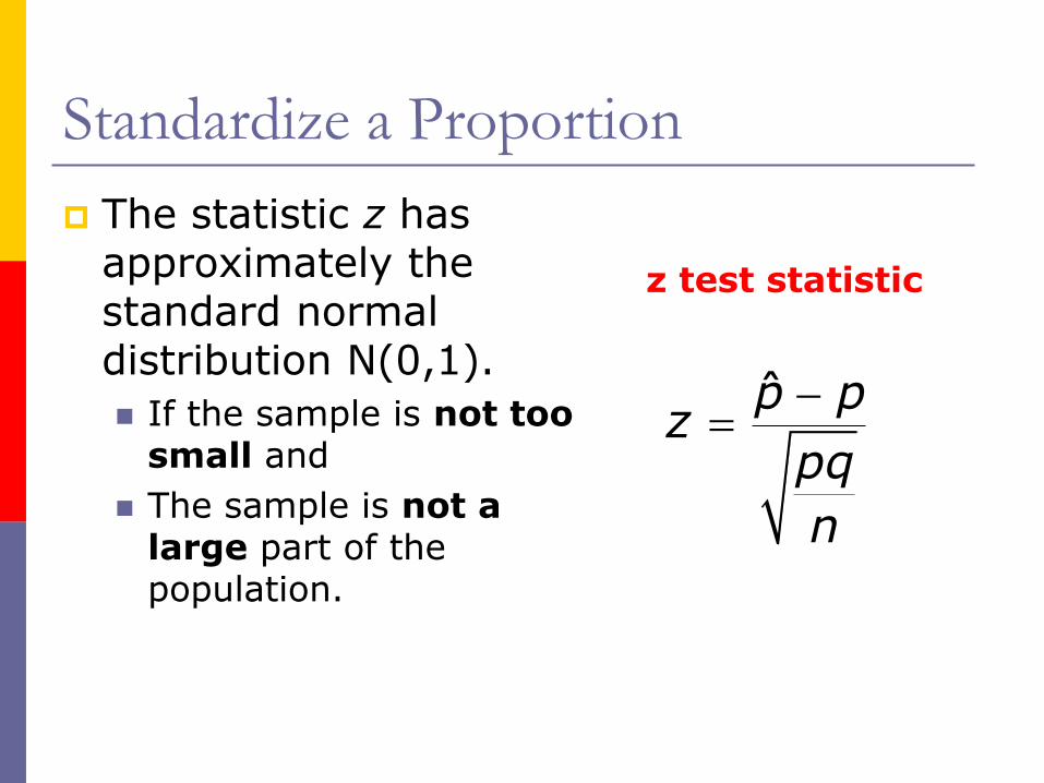
Standardize a Proportion
The statistic z has approximately the standard normal distribution N(0,1).
If the sample is not too small and
The sample is not a large part of the population.
p̂ pz
pq
n
z test statistic

Conditions for Inference about a
Proportion
The data are an SRS from the population of interest.
The population is at least 10 times as large as the sample.
Population 10
For a hypothesis test Ho: p=po, the sample size n is so large that both are:
npo 10 and
nqo 10
For a confidence interval, n is so large that both are:
n 10
n 10
p̂
q̂
Confidence Interval for a Proportion
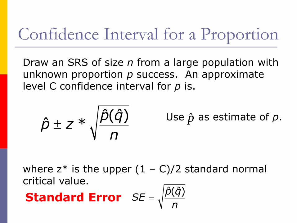
Draw an SRS of size n from a large population with unknown proportion p success. An approximate level C confidence interval for p is.
( )ˆ ˆ
*ˆp q
p zn
where z* is the upper (1 – C)/2 standard normalcritical value.
Standard Error ( )ˆ ˆp q
SEn
Use as estimate of p.p̂
Margin of Error and Sample size
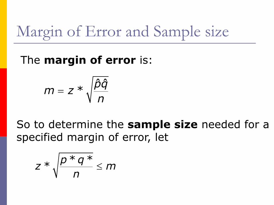
The margin of error is:
ˆˆ
*pq
m zn
So to determine the sample size needed for aspecified margin of error, let
* *
*p q
z mn

Example – Confidence Interval
In May 2002, the Gallup Poll ask 537 randomly sampled adults the question “Generally speaking, do you believe the death penalty is applied fairly or unfairly in this country today?” Of these, 53% answered “Fairly and 7% said they didn’t know. What can we conclude from this survey?
Step 1 – Identify the population of interest and parameter you want to draw conclusions about.
p = , of U.S. adults who think the death penalty is applied fairly.
53%40%
7%
Fairly
Unfarily
Don't Know
Example – Confidence Interval
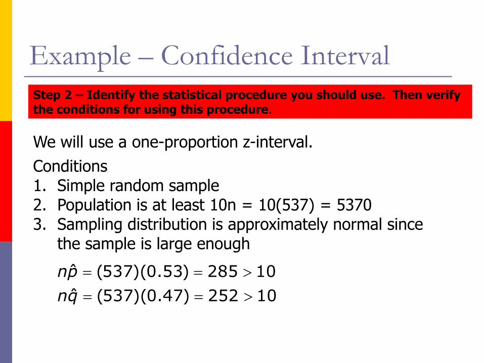
Step 2 – Identify the statistical procedure you should use. Then verify the conditions for using this procedure.
We will use a one-proportion z-interval.
Conditions 1. Simple random sample2. Population is at least 10n = 10(537) = 53703. Sampling distribution is approximately normal since
the sample is large enough
(537)(0.53) 285 10ˆ
(537)(0.47) 252 10ˆ
np
nq

Example – Confidence Interval
ˆˆ
*ˆpq
p zn
0.53 537 284.61 285x
Example – Confidence Interval
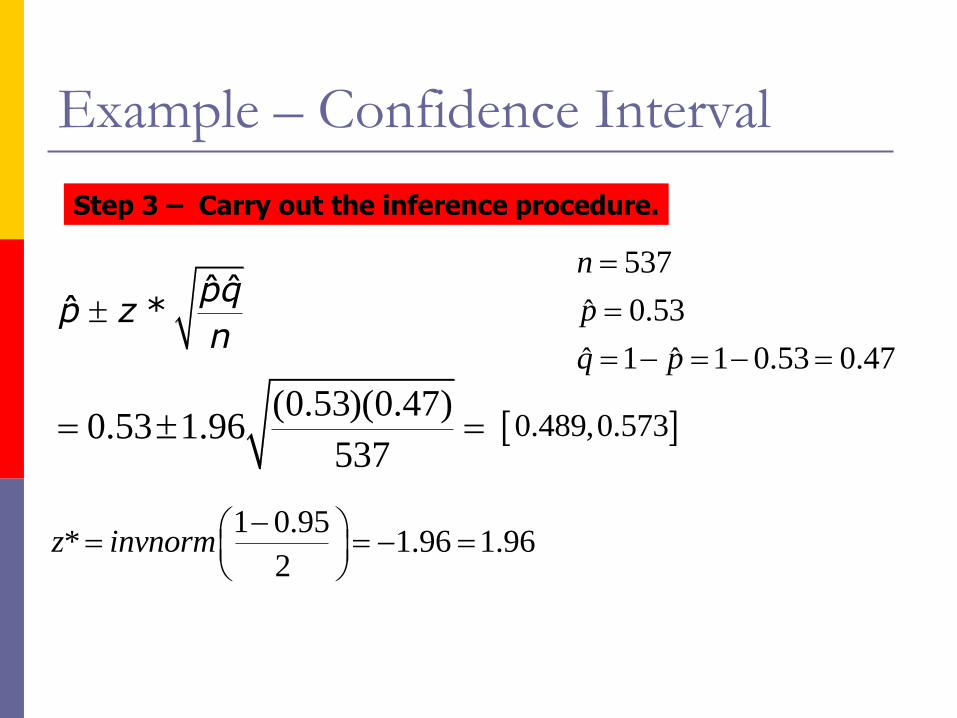
Step 3 – Carry out the inference procedure.
ˆˆ
*ˆpq
p zn
(0.53)(0.47)0.53 1.96
537
1 0.95* 1.96 1.96
2z invnorm
537
0.53ˆ
1 1 0.53 0.47ˆ ˆ
n
p
q p
0.489,0.573
Example – Confidence Interval
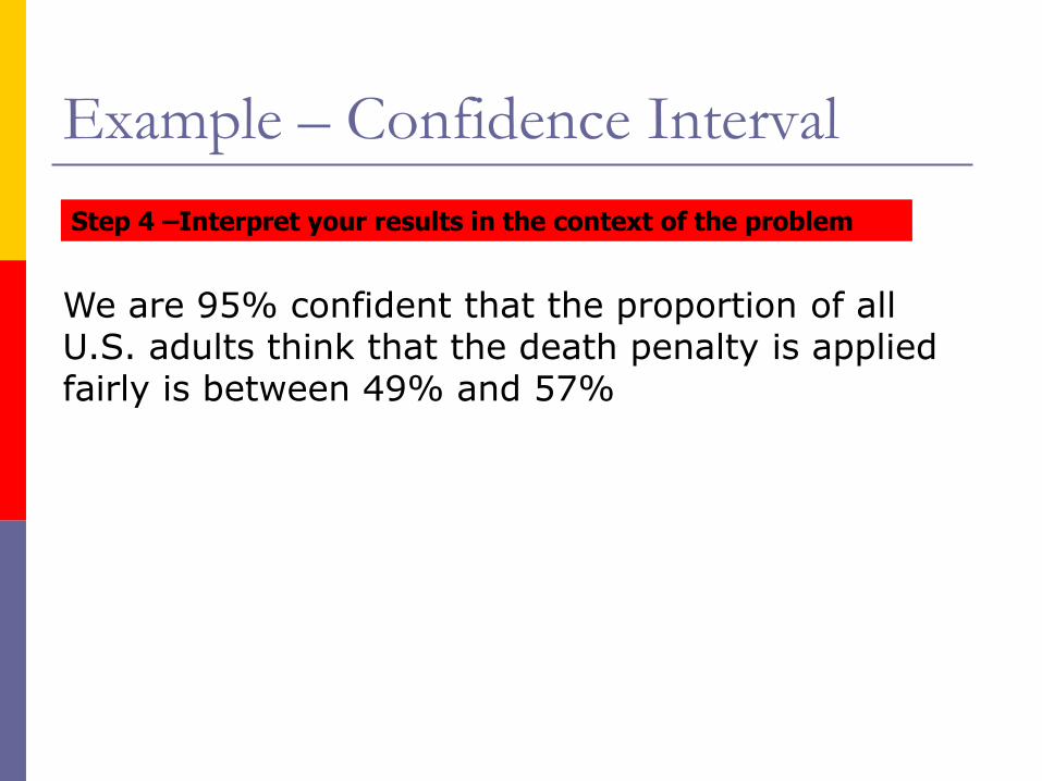
Step 4 –Interpret your results in the context of the problem
We are 95% confident that the proportion of all U.S. adults think that the death penalty is applied fairly is between 49% and 57%
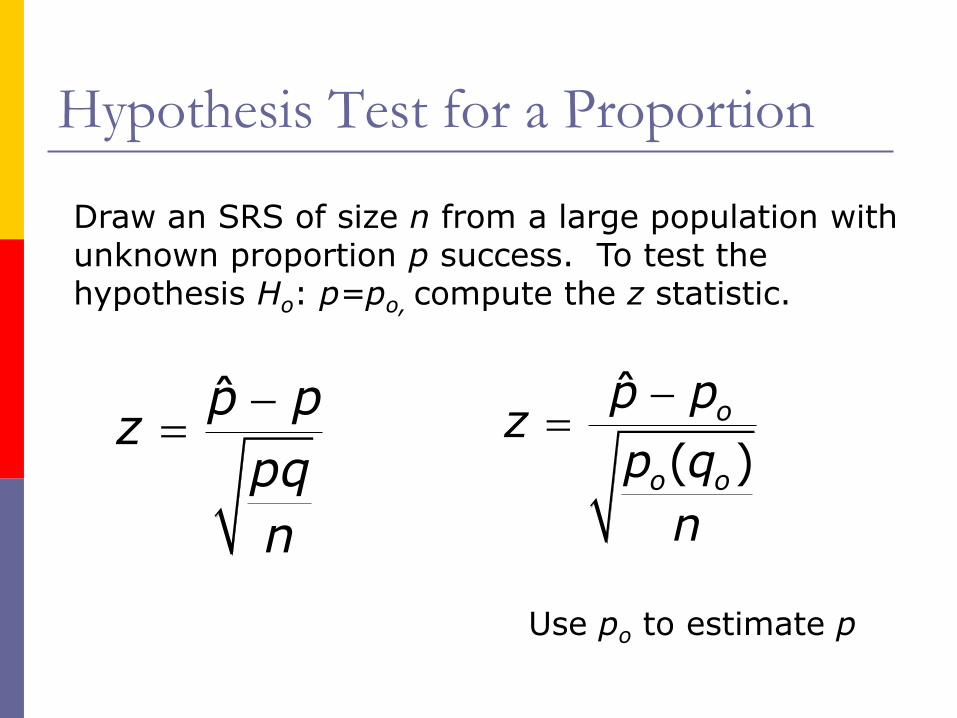
Hypothesis Test for a Proportion
Draw an SRS of size n from a large population with unknown proportion p success. To test the hypothesis Ho: p=po, compute the z statistic.
ˆ
( )
o
o o
p pz
p q
n
p̂ pz
pq
n
Use po to estimate p
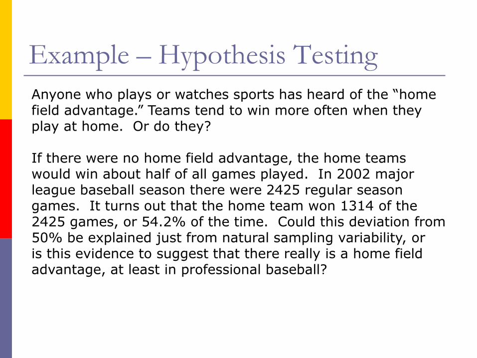
Example – Hypothesis Testing
Anyone who plays or watches sports has heard of the “homefield advantage.” Teams tend to win more often when theyplay at home. Or do they?
If there were no home field advantage, the home teamswould win about half of all games played. In 2002 majorleague baseball season there were 2425 regular seasongames. It turns out that the home team won 1314 of the 2425 games, or 54.2% of the time. Could this deviation from50% be explained just from natural sampling variability, oris this evidence to suggest that there really is a home fieldadvantage, at least in professional baseball?
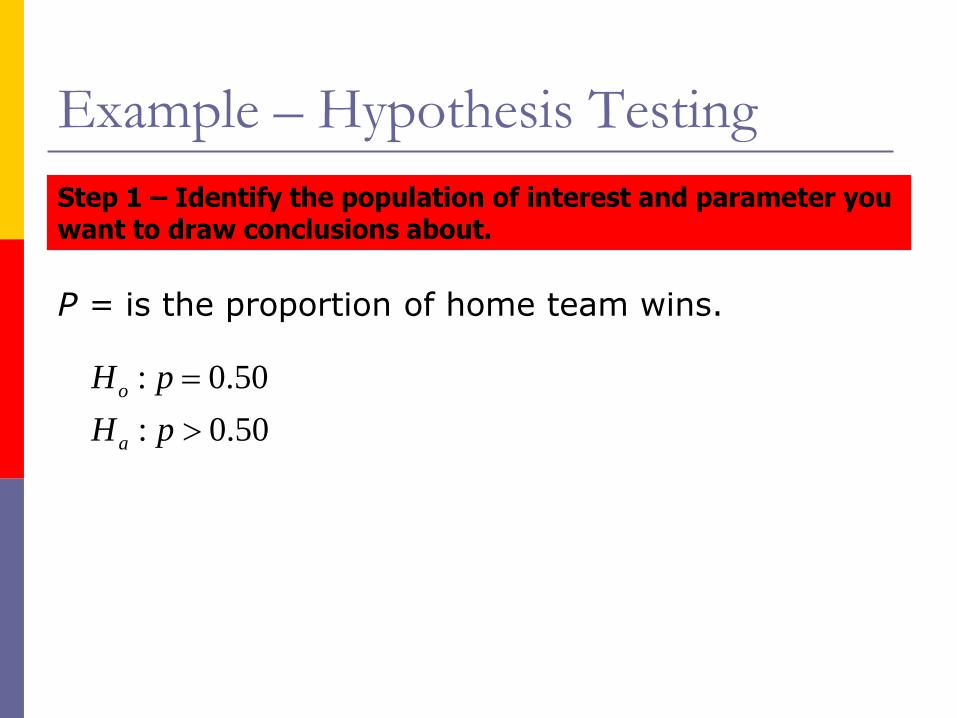
Example – Hypothesis Testing
Step 1 – Identify the population of interest and parameter you want to draw conclusions about.
P = is the proportion of home team wins.
: 0.50
: 0.50
o
a
H p
H p
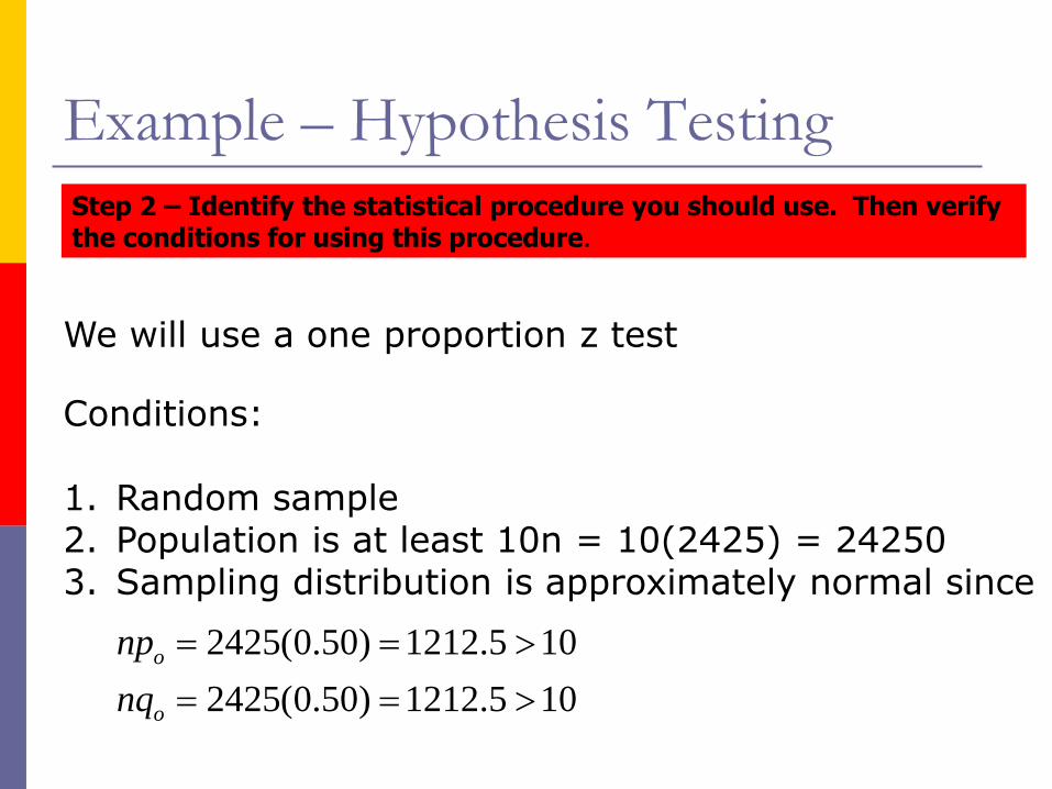
Example – Hypothesis Testing
We will use a one proportion z test
Step 2 – Identify the statistical procedure you should use. Then verify the conditions for using this procedure.
Conditions:
1. Random sample2. Population is at least 10n = 10(2425) = 242503. Sampling distribution is approximately normal since
2425(0.50) 1212.5 10
2425(0.50) 1212.5 10
o
o
np
nq
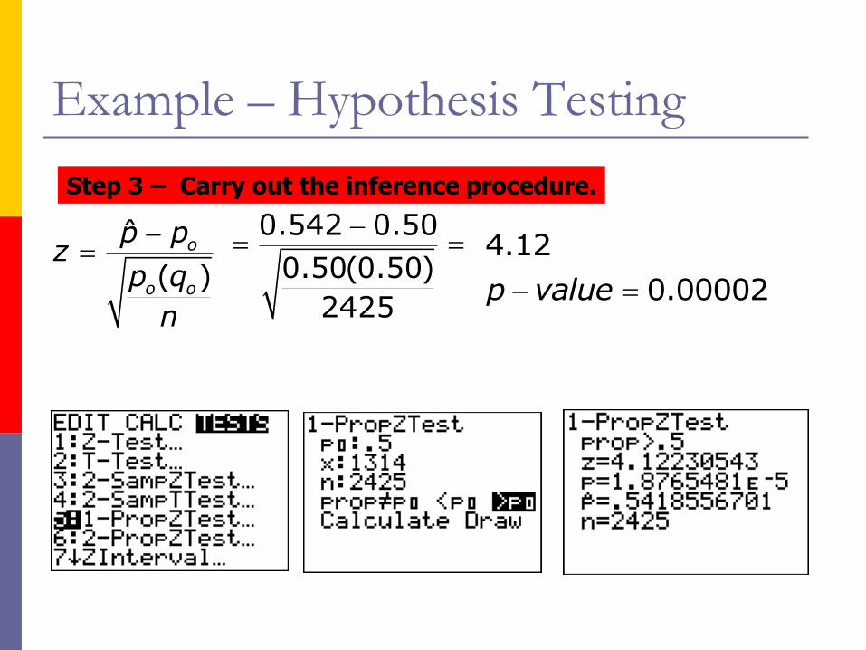
Example – Hypothesis Testing
ˆ
( )
o
o o
p pz
p q
n
0.542 0.50
0.50(0.50)
2425
4.12
0.00002p value
Step 3 – Carry out the inference procedure.
Example – Hypothesis Testing
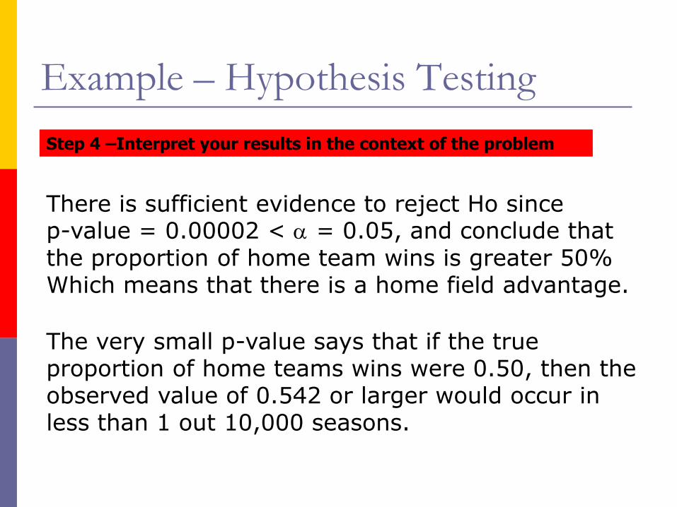
Step 4 –Interpret your results in the context of the problem
There is sufficient evidence to reject Ho since p-value = 0.00002 < = 0.05, and conclude that the proportion of home team wins is greater 50% Which means that there is a home field advantage.
The very small p-value says that if the true proportion of home teams wins were 0.50, then theobserved value of 0.542 or larger would occur inless than 1 out 10,000 seasons.
Lesson 12-2
Comparing Two Proportions
Comparing Two Populations
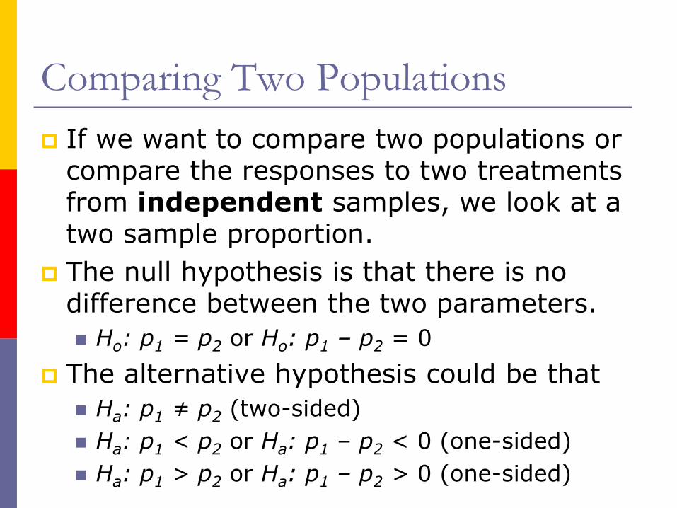
If we want to compare two populations or compare the responses to two treatments from independent samples, we look at a two sample proportion.
The null hypothesis is that there is no difference between the two parameters.
Ho: p1 = p2 or Ho: p1 – p2 = 0
The alternative hypothesis could be that
Ha: p1 ≠ p2 (two-sided)
Ha: p1 < p2 or Ha: p1 – p2 < 0 (one-sided)
Ha: p1 > p2 or Ha: p1 – p2 > 0 (one-sided)
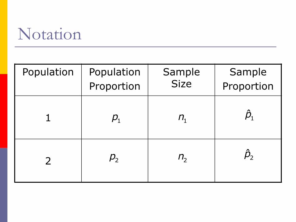
Notation
Population Population
Proportion
Sample Size
Sample
Proportion
1
2
1p
2p
1n
2n
1̂p
2̂p
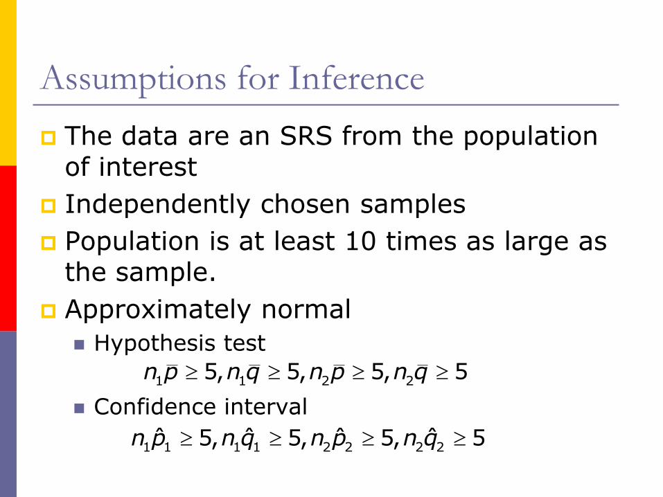
Assumptions for Inference
The data are an SRS from the population of interest
Independently chosen samples
Population is at least 10 times as large as the sample.
Approximately normal
Hypothesis test
Confidence interval
1 1 1 1 2 2 2 25, 5, 5, 5ˆ ˆ ˆ ˆn p n q n p n q
1 1 2 25, 5, 5, 5n p n q n p n q
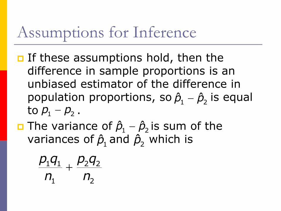
Assumptions for Inference
If these assumptions hold, then the difference in sample proportions is an unbiased estimator of the difference in population proportions, so is equal to .
The variance of is sum of the variances of and which is
1 2ˆ ˆp p
1 2p p
1 2ˆ ˆp p
1̂p 2̂p
1 1 2 2
1 2
p q p q
n n
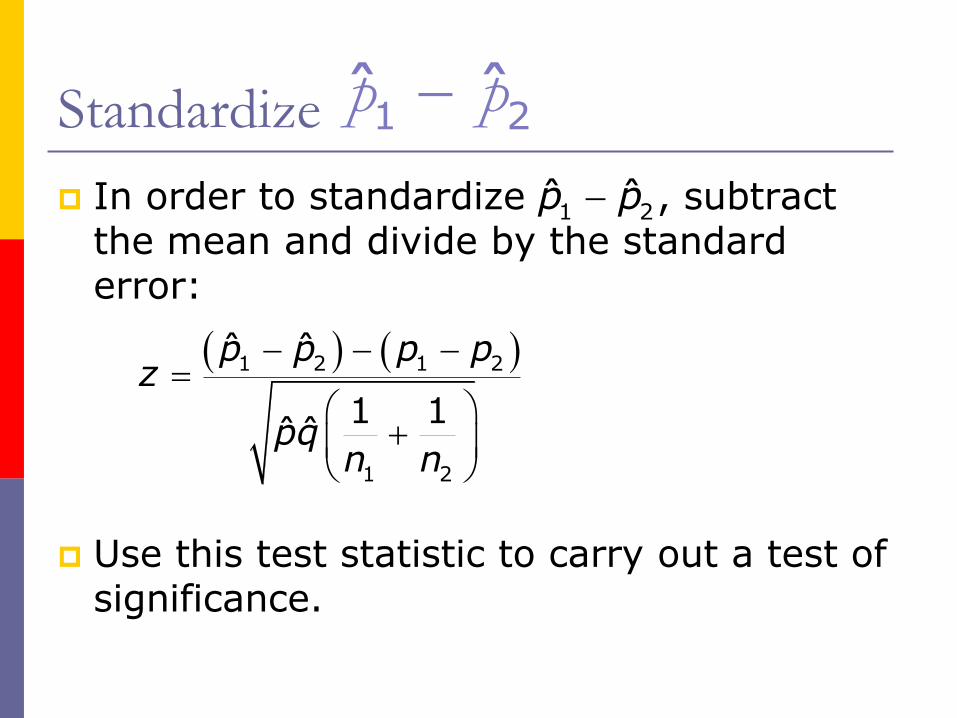
Standardize
In order to standardize , subtract the mean and divide by the standard error:
Use this test statistic to carry out a test of significance.
1 2ˆ ˆp p
1 2ˆ ˆp p
1 2 1 2
1 2
ˆ ˆ
1 1ˆˆ
p p p pz
pqn n
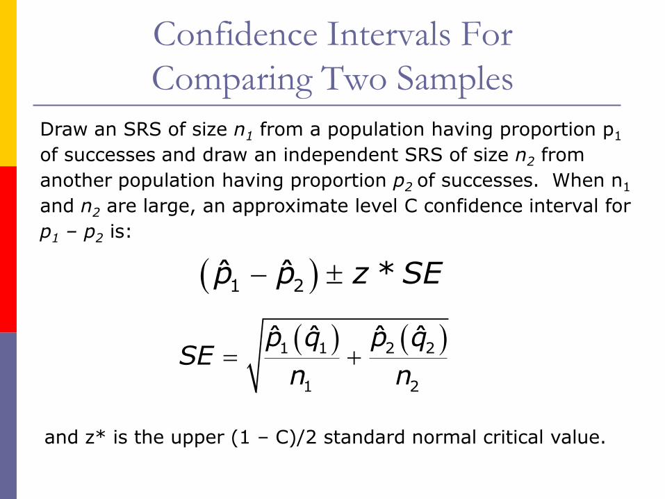
Confidence Intervals For
Comparing Two Samples
Draw an SRS of size n1 from a population having proportion p1
of successes and draw an independent SRS of size n2 from
another population having proportion p2 of successes. When n1
and n2 are large, an approximate level C confidence interval for
p1 – p2 is:
1 2 *ˆ ˆp p z SE
1 1 2 2
1 2
ˆ ˆ ˆ ˆp q p qSE
n n
and z* is the upper (1 – C)/2 standard normal critical value.
Example – Confidence Interval
Who are typically more intelligent, men or women? To find out what people think, the Gallup Poll selected a random sample of 520 women and asked them to indicate whether each attribute was, “generally more true of men or women.” When asked about intelligence, 28% of the men thought men were generally more intelligent, but only 14% of the women agreed. Is there a gender gap in opinions about which sex is smarter? Use a 95% confidence interval to estimate the true size of that gap to be?
Example – Confidence Interval
pm – pf = difference in the population proportion, (pm), of American men who think that men can be described as “intelligent” and the proportion, (pf), of American women who think so.
Step 1 – Identify the population of interest and parameter you want to draw conclusions about.
Example – Confidence Interval
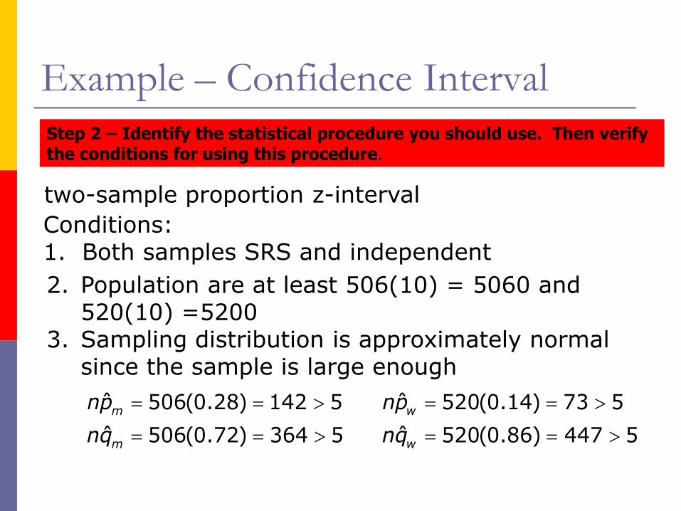
two-sample proportion z-interval
Conditions:1. Both samples SRS and independent
2. Population are at least 506(10) = 5060 and 520(10) =5200
3. Sampling distribution is approximately normal since the sample is large enough
Step 2 – Identify the statistical procedure you should use. Then verify the conditions for using this procedure.
506(0.28) 142 5ˆ
506(0.72) 364 5ˆ
m
m
np
nq
520(0.14) 73 5ˆ
520(0.86) 447 5ˆ
w
w
np
nq

Example – Confidence Interval
506, 520
0.28, 0.14ˆ ˆ
M F
M F
n n
p p
0.28(0.72) 0.14(0.86)
0.28 0.14 1.96506 520
(506)(0.28) 141.68 142
(520)(0.14) 72.8 73
M
F
x
x
0.14 0.049 [0.091,0.189]
Example – Confidence Interval
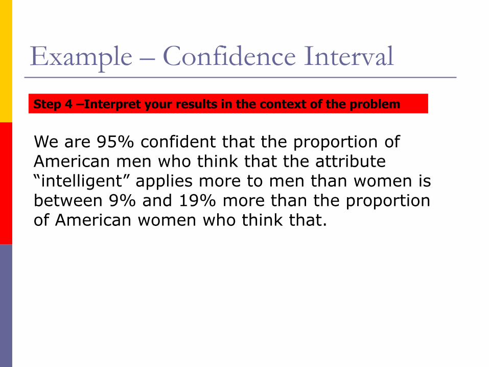
We are 95% confident that the proportion of American men who think that the attribute “intelligent” applies more to men than women isbetween 9% and 19% more than the proportionof American women who think that.
Step 4 –Interpret your results in the context of the problem
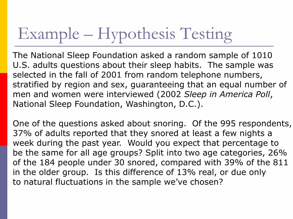
Example – Hypothesis TestingThe National Sleep Foundation asked a random sample of 1010U.S. adults questions about their sleep habits. The sample was selected in the fall of 2001 from random telephone numbers, stratified by region and sex, guaranteeing that an equal number of men and women were interviewed (2002 Sleep in America Poll, National Sleep Foundation, Washington, D.C.).
One of the questions asked about snoring. Of the 995 respondents,37% of adults reported that they snored at least a few nights aweek during the past year. Would you expect that percentage tobe the same for all age groups? Split into two age categories, 26%of the 184 people under 30 snored, compared with 39% of the 811in the older group. Is this difference of 13% real, or due onlyto natural fluctuations in the sample we’ve chosen?
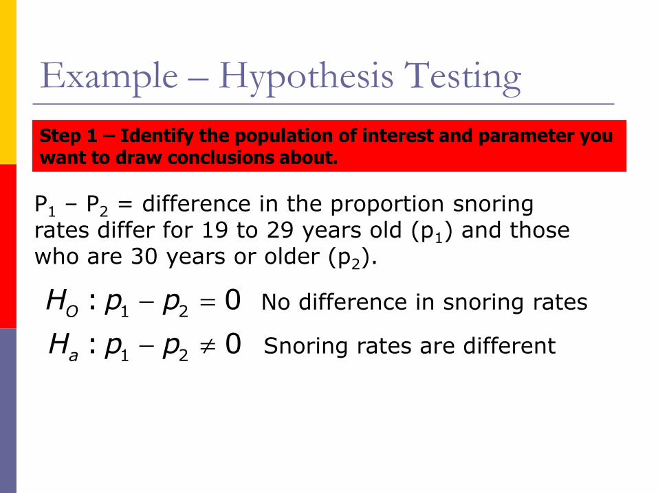
Example – Hypothesis Testing
Step 1 – Identify the population of interest and parameter you want to draw conclusions about.
P1 – P2 = difference in the proportion snoring rates differ for 19 to 29 years old (p1) and those who are 30 years or older (p2).
1 2
1 2
: 0
: 0
O
a
H p p
H p p
No difference in snoring rates
Snoring rates are different
Example – Hypothesis Testing
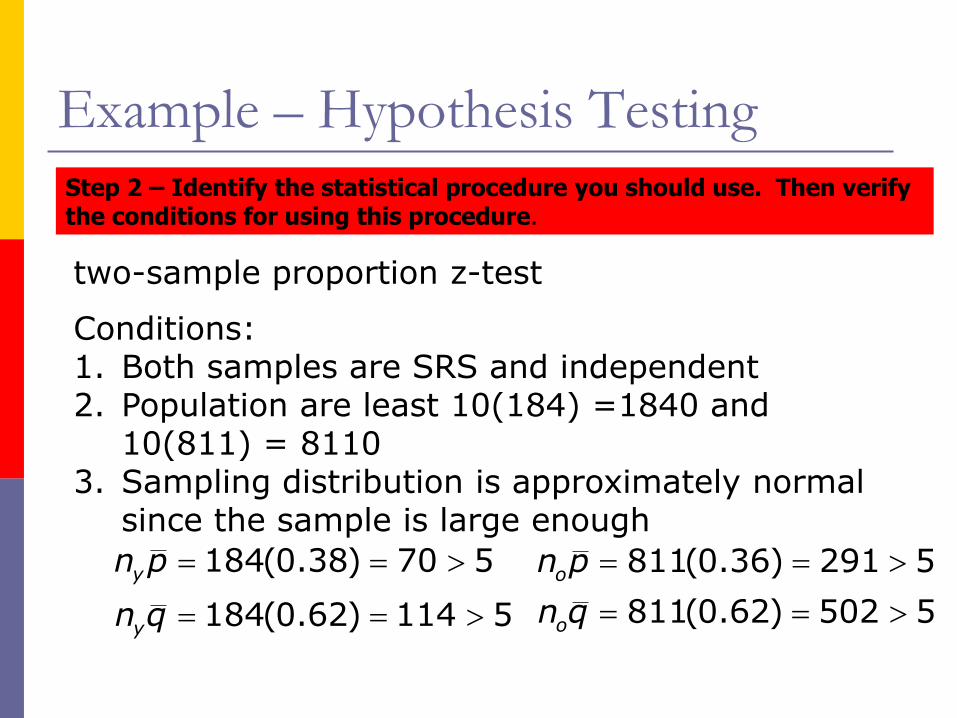
Step 2 – Identify the statistical procedure you should use. Then verify the conditions for using this procedure.
two-sample proportion z-test
Conditions:1. Both samples are SRS and independent2. Population are least 10(184) =1840 and
10(811) = 81103. Sampling distribution is approximately normal
since the sample is large enough
184(0.38) 70 5
184(0.62) 114 5
y
y
n p
n q
811(0.36) 291 5
811(0.62) 502 5
o
o
n p
n q
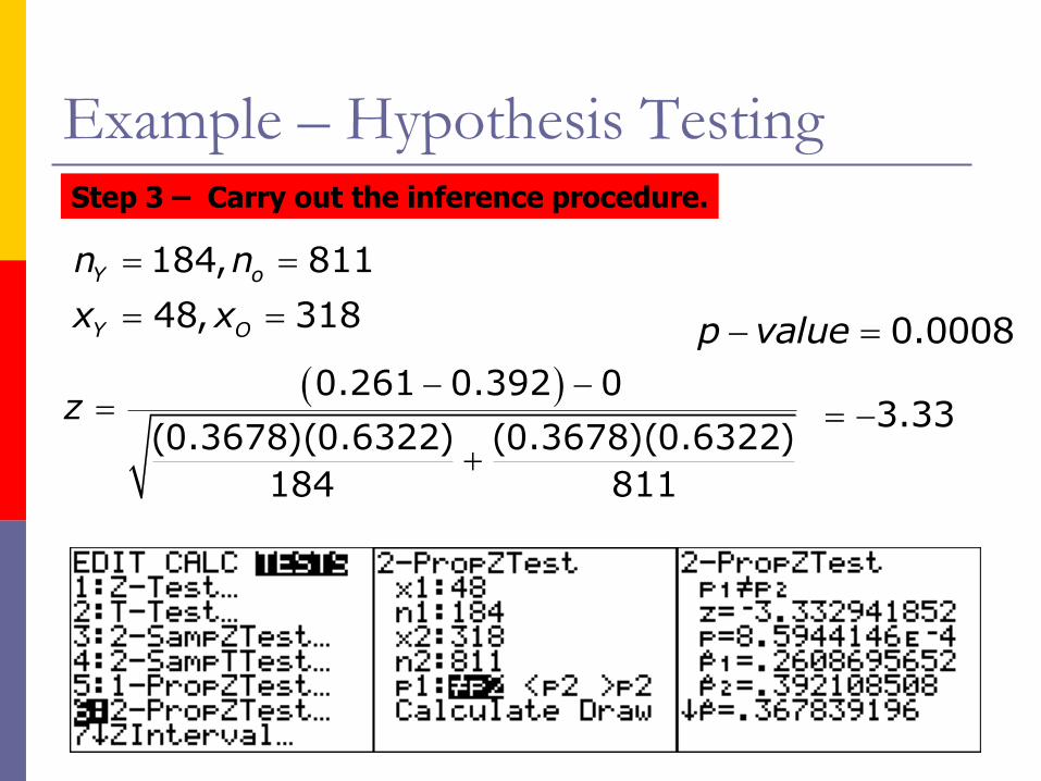
Example – Hypothesis Testing
184, 811
48, 318
Y o
Y O
n n
x x
0.261 0.392 0
(0.3678)(0.6322) (0.3678)(0.6322)
184 811
z
3.33
0.0008p value
Step 3 – Carry out the inference procedure.
Example – Hypothesis Testing
Step 4 –Interpret your results in the context of the problem
There is sufficient evidence to reject Ho. Sincep-value = 0.0008 < = 0.05 and conclude that there is a difference in the rate of snoring between older adults and younger adults. It appears that older adults are more likely to snore.
The p-value of 0.0008 says that if there is reallyno difference in snoring rates between the two agegroups, then the difference observed in this studywould happen only 8 times in 10,000. This is rareenough for us to reject the null hypothesis.