Chapter 12wpscms.pearsoncmg.com/wps/media/objects/15089/15451222/notes/...• Explain the key determinants of consumption and saving in the Keynesian ... – The interest rate is not

1

Chapter 12

Consumption, Real GDP, and the Multiplier

Copyright ©2014 Pearson Education, Inc. All rights reserved. 12-2

Introduction

Since the early 2000s, planned real investment spending has increased in most of the world’s nations.

As a percentage of global real GDP, however, planned real investment spending in the world’s developed countries has declined. Yet, it has been rising in emerging-economy nations. These are countries transitioning to a developed status.

How do changes in planned real investment spending affect a country’s real GDP?

Reading Chapter 12 will help you answer this question.


Learning Objectives

• Distinguish between saving and savings and explain how consumption and saving are related

• Explain the key determinants of consumption and saving in the Keynesian model

• Identify the primary determinants of planned investment

2


Learning Objectives (cont'd)

• Describe how equilibrium real GDP is established in the Keynesian model

• Evaluate why autonomous changes in total planned expenditures have a multiplier effect on equilibrium real GDP

• Understand the relationship between total planned expenditures and the aggregate demand curve


Chapter Outline

• Some Simplifying Assumptions in a Keynesian Model

• Determinants of Planned Consumption and Planned Saving

• Determinants of Investment• Determining Equilibrium Real GDP


Chapter Outline (cont'd)

• Keynesian Equilibrium with Government and the Foreign Sector Added

• The Multiplier• How a Change in Real Autonomous

Spending Affects Real GDP When the Price Level Can Change

• The Relationship Between Aggregate Demand and the C + I + G + X Curve

3


Did You Know That ...

• The share of real GDP allocated to real consumption spending is:– 66 percent in Germany– 60 percent in the United Kingdom– 70 percent in the United States– Less than 41 percent in China?

• In this chapter, you will learn how an understanding of households’ real saving and real consumption spending can help you evaluate fluctuations in a national’s real GDP.


Some Simplifying Assumptions in a Keynesian Model

• To simplify the income determination model, let’s assume:1. Businesses pay no indirect taxes (sales tax)

2. Businesses distribute all profits to shareholders

3. There is no depreciation

4. The economy is closed; no foreign trade


Some Simplifying Assumptions in a Keynesian Model (cont'd)

• Real Disposable Income– Real GDP minus net taxes, or after-tax real

income

• Consumption– Spending on new goods and services out of a

household’s current income– Whatever is not consumed is saved– Consumption includes such things as buying

food and going to a concert

4



• Saving– The act of not consuming all of one’s current

income

– Whatever is not consumed out of spendable income is, by definition, saved

– Saving is an action measured over time (a flow)

– Savings are a stock, an accumulation resulting from the act of saving in the past



• Consumption Goods– Goods bought by households to use up, such as

food and movies



• Accounting identity:

Consumption + saving disposable income

Saving disposable income – consumption

5



• Investment– Spending by businesses on things such as

machines and buildings, which can be used to produce goods and services in the future

– The investment part of real GDP is the portion that will be used in the process of producing goods in the future



• Capital Goods– Producer durables; nonconsumable goods that

firms use to make other goods


Determinants of Planned Consumption and Planned Saving

• In the classical model, the supply of saving was determined by the rate of interest– The higher the rate, the more people wanted to

save, and the less they wanted to consume

6


Determinants of Planned Consumption and Planned Saving (cont'd)

• Keynes argued that: – The interest rate is not the most important

factor in saving and consumption decisions– Rather, real saving and consumption decisions

depend primarily on a household’s real disposable income.

– Furthermore, a person’s anticipation about future flows of income influences how much of current income is allocated to consumption and how much is allocated to saving.



• The Life-Cycle Theory of Consumption– The most realistic and detailed theory of consumption,

often called the life-cycle theory of consumption, considers how a person varies saving and consumption as income ebbs and flows throughout an entire life span.

• This theory predicts that when an individual anticipates a higher income in the future, he or she will tend to consume more and save less in the current period than would have been the case otherwise.



• The Permanent Income Hypothesis– A related theory, called the permanent income hypothesis,

suggests that the income level that matters for a person’s decisions about current consumption and saving is permanent income, or expected average lifetime income.

• Thus, if a person’s flow of income temporarily rises without an increase in average lifetime income, the person responds by saving more and leaving consumption unchanged.

7



• The Keynesian Theory of Consumption and Saving– Keynes argued that real consumption and saving

decisions depend primarily on a household’s current real disposable income.



• Consumption Function– The relationship between amount consumed and

disposable income

– A consumption function tells us how much people plan to consume at various levels of disposable income



• Dissaving– Negative saving; a situation in which spending

exceeds income

– Dissaving can occur when a household is able to borrow or use up existing assets

8


Table 12-1 Real Consumption and Saving Schedules: A Hypothetical Case



• 45-Degree Reference Line– The line along which planned real expenditures

equal real GDP per year


Figure 12-1The Consumption and Saving Functions

9



• Autonomous Consumption– The part of consumption that is independent of

the level of disposable income

– Changes in autonomous consumption shift the consumption function



• Average Propensity to Consume (APC)– Real consumption divided by real disposable

income

– The proportion of total disposable income that is consumed

APC =Real consumption

Real disposable income



• Average Propensity to Save (APS)– Real saving divided by real disposable income

(DI)

– Saved proportion of real DI

APS =Real saving

Real disposable income

10


MPC =Change in real consumption

Change in real disposable income


• Marginal Propensity to Consume (MPC)– The ratio of the change in real consumption to

the change in real disposable income


MPS =Change in real saving

Change in real disposable income


• Marginal Propensity to Save (MPS)– The ratio of the change in saving to the change

in disposable income


APC =$49,200

$54,000= .911


• Example– Income = $54,000– C = $49,200– S = $4,800

• What is the APC?

11


APC =$54,000

$60,000= .90


• Example– Income increases by $6,000 to $60,000– C = $54,000– S = $6,000

• What is the APC?



• Some relationships

APC + APS 1

MPC + MPS 1



• Causes of shifts in the consumption function– A change besides real disposable income will

cause the consumption function to shift

– Non-income determinants of consumption• Population• Wealth

12



• Net wealth– The stock of assets owned by a person,

household, firm or nation (net of any debts owed)

– For a household, wealth can consist of a house, cars, personal belongings, stocks, bonds, bank accounts, and cash (minus any debts owed)


Example: Lower Household Wealth and Subdued Growth in Consumption

• Between 2007 and 2009, there was a substantial decline in two key components of real household wealth.– Inflation-adjusted wealth in housing fell by 25 percent

– Inflation-adjusted wealth in corporate stocks fell by 50 percent

• These wealth reductions shifted the U.S. consumption function downward.

• Real disposable income also fell, causing a leftward movement along the consumption function and a further drop in consumption.


Determinants of Investment

• Investment, you will remember, consists of expenditures on new buildings and equipment– Gross private domestic investment has been

volatile

– Consider the planned investment function, and shifts in the function

13


Figure 12-2 Planned Real Investment, Panel (a)


Figure 12-2 Planned Real Investment, Panel (b)


Example: Adding a Third Dimension Requires New Investment Spending

• Of the approximately 40,000 movie screens in the United States, fewer than 8,000 are equipped with digital technology required for projection of three-dimensional (3D) movies.

• Conversion to the 3D technology costs about $70,000.

• Major movie-theater chains are currently undertaking this investment for more than 1,000 theaters.

• This adds up to an aggregate investment expenditure of about $700 million.

14


Determining Equilibrium Real GDP

• We are interested in determining the equilibrium level of real GDP per year– Consumption as a function of real GDP

– The 45-degree reference line


Figure 12-3 Consumption as a Function of Real GDP


Determining Equilibrium Real GDP (cont'd)

• Adding the investment function

AD = C + I + G + X

15


Figure 12-4 Combining Consumption and Investment



• Saving and investment: Planned versus Actual – Only at equilibrium real GDP will planned saving

equal actual saving

– Planned investment equals actual investment

– Hence planned saving is equal to planned investment


Figure 12-5 Planned and Actual Rates of Saving and Investment

16



• Unplanned increases in business inventories– Consumers purchase fewer goods and services

than anticipated

– This leaves firms with unsold products and inventories will rise

– Businesses respond by cutting back production and reducing employment



• Unplanned decreases in business inventories– Business will increase production of goods and

services and increase employment

– Ultimately there will be an increase in real GDP


Keynesian Equilibrium with Government and the Foreign Sector Added

• To this point we have ignored the role of government in our model

• We also left out the foreign sector of the economy in our model

• Let’s think about what happens when we add these elements

17


Keynesian Equilibrium with Government and the Foreign Sector Added (cont'd)

• Government (G): C + I + G– Federal, state, and local

• Does not include transfer payments• Is autonomous• Lump-sum taxes = G

• Lump-Sum Tax– A tax that does not depend on income or the

circumstances of the taxpayer



• The Foreign Sector: C + I + G + X– Net exports (X) equals exports minus imports

– Depends on international economic conditions

– Autonomous—independent of real national income


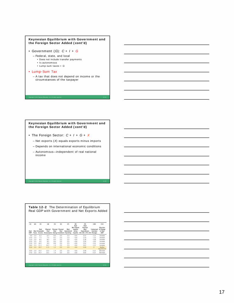
Table 12-2 The Determination of Equilibrium Real GDP with Government and Net Exports Added

18



• Determining the equilibrium level of GDP per year– We are now in a position to determine the

equilibrium level of real GDP per year

– Remember that equilibrium always occurs when total planned real expenditures equal real GDP


Figure 12-6 The Equilibrium Level of Real GDP



The Equilibrium Level of Real GDP• Observations

– If C + I + G + X = Y • Equilibrium GDP

– If C + I + G + X > Y• Unplanned decrease in inventories• Businesses raise output• Y returns to equilibrium

– If C + I + G + X < Y• Unplanned increase in inventories• Businesses reduce output• Y returns to equilibrium

19


The Multiplier

• Multiplier– The ratio of the change in the equilibrium level

of real national income to the change in autonomous expenditures

– The number by which a change in autonomous real investment or autonomous real consumption is multiplied to get the change in equilibrium real GDP


The Multiplier (cont'd)

• Question– How can a $100 billion increase in investment

generate a $500 billion increase in equilibrium real GDP?

• Answer– The multiplier process


Table 12-3 The Multiplier Process

20



• The multiplier formula

Multiplier = 11 - MPC

= 1MPS



• By taking a few numerical examples, you can demonstrate to yourself an important property of the multiplier– The smaller the MPS, the larger the multiplier

– The larger the MPC, the larger the multiplier



• Examples

MPC =4

5MPS =

1

5Multiplier =

1

1/5= 5

MPC =3

5MPS =

2

5Multiplier =

1

2/5= 2.5

21


Change in equilibrium real GDP = Multiplier x Change in autonomous spending


• Measuring the change in equilibrium income from a change in autonomous spending



• Significance of the multiplier– It is possible that a relatively small change in

consumption or investment can trigger a much larger change in real GDP


What If . . . The government seeks a larger multiplier effect by funding private spending on certain items rather than buying them directly?

• Whether the government gives funds to households and firms for purchasing goods or whether the government makes the purchases directly, the resulting increase in total autonomous expenditure is the same.– Thus, the overall multiplier effect on equilibrium

real GDP would also be the same.– So, providing grants of public funds to be spent

by households and firms rather than having government purchase the same items will not enlarge the overall theoretical multiplier effect.

22


How a Change in Real Autonomous Spending Affects Real GDP When the Price Level Can Change

• So far our examination of how changes in real autonomous spending affects equilibrium real GDP has considered a situation in which the price level remains unchanged

• Our equilibrium analysis has only considered how AD shifts in response to investment, government spending, net exports


How a Change in Real Autonomous Spending Affects Real GDP When the Price Level Can Change (cont'd)

• When we take into account the aggregate supply curve, we must also consider responses of the equilibrium price level to a multiplier-induced change in AD


Figure 12-7 Effect of a Rise in Autonomous Spending on Equilibrium Real GDP

23


International Example: The Effect of Higher Autonomous Spending on China’s Real GDP

• Most estimates indicate that the marginal propensity to consume in China is about 0.50.

• So, assuming no change in the price level, the multiplier would be about 2.

• However, economists have estimated that the short-run effect of an initial increase in real autonomous spending on China’s real GDP is only about 1.1.

• Therefore, once the higher price level is taken into account, an additional one-unit increase in real autonomous expenditure causes a 1.1 unit increase in China’s annual real GDP.


The Relationship Between Aggregate Demand and the C + I + G + X Curve

• Aggregate demand consists of: – Consumption

– Investment

– Government

– Foreign sector


The Relationship Between Aggregate Demand and the C + I + G + X Curve (cont'd)

• There is a major difference between the two: – C + I + G + X curve drawn with price level

constant

– AD curve drawn with the price level changing

• To derive the aggregate demand curve from the C + I + G + X curve, we must now allow the price level to change

24


The Relationship Between Aggregate Demand and the C + I + G + X Curve (cont'd)

• What are some of the effects of a price level increase?– Real balance effect

– Interest rate effect

– The open economy effect


Figure 12-8 The Relationship Between AD and the C + I + G+ X Curve


You Are There: Evaluating the Effects of Declining Real Disposable Income

• Mark Vitner, an economist with Wells Fargo bank, examines the latest monthly economic data.

• Real disposable income fell by 0.3 percent during the month.

• Real consumption spending and real saving dipped as well, consistent with the theory.

• Vitner summarizes the situation by saying that household budgets are getting tighter and consumers are having difficulty maintaining their standard of living.

25


Issues & Applications: A Global Reversal in Planned Investment Spending

• In the past, developed countries have displayed the largest upward shifts in their planned investment functions.

• Recently, however, larger upward shifts have occurred among the emerging-economy nations, such as China, India, South Korea, and Singapore.

• Figure 12-9 on the next slide displays real investment spending as a percentage of global real GDP for developed and emerging nations.


Figure 12-9 Real Investment Spending as a Percentage of Global Real GDP in Two Groups of Nations since 1995

Sources: International Monetary Fund; author’s estimates.


Issues & Applications: A Global Reversal in Planned Investment Spending (cont’d)

• Variations in planned real investment spending operate through the multiplier to bring about changes in equilibrium real GDP.

• Therefore, a country that experiences a larger upward shift in its planned investment function will observe a greater increase in its equilibrium real GDP.

• This explains why countries such as China, India, South Korea, and Singapore are emerging to take a place alongside developed nations.

26


Summary Discussion of Learning Objectives

• The difference between saving and savings and the relationship between saving and consumption – Saving is a flow over time while savings is a

stock

– Consumption plus saving equals disposable income


Summary Discussion of Learning Objectives (cont'd)

• Key determinants of consumption and saving in the Keynesian model– In the classical model, the interest rate is the

fundamental determinant of saving

– In the Keynesian model, the primary determinant is disposable income

– DI increases, so does C



• The key determinants of planned investment– The interest rate, business expectations,

productive technology, and business taxes

27



• How equilibrium real GDP is established in the Keynesian model – Equilibrium national income occurs where the C

+ I + G + X schedule crosses the 45-degree line



• Why autonomous changes in total planned expenditures have a multiplier effect on equilibrium real GDP– As consumption increases, so does real GDP,

which induces further consumption spending

– The ultimate expansion of real GDP is equal to the multiplier times the increase in autonomous expenditures



• The relationship between total planned expenditures and the aggregate demand curve – AD consists of consumption, investment, and

government purchases, plus the foreign sector

– Difference• C + I + G + X curve drawn with price level constant• AD with the price level changing

28


Figure C-1 Graphing the Multiplier

Documents

Chapter 12wpscms.pearsoncmg.com/wps/media/objects/15089/15451222/notes/...• Explain the key determinants of consumption and saving in the Keynesian ... – The interest rate is not