CHAPTER Discrete Fourier Transform and Signal …jan/dsp/Note/Example-DFT-FFT.pdf · 90 CHAPTER 4 Discrete Fourier Transform and Signal Spectrum. ... We can use MATLAB functions fft()

Discrete Fourier Transform andSignal Spectrum 4CHAPTER OUTLINE

4.1 Discrete Fourier Transform.............................................................................................................. 87

4.1.1 Fourier Series Coefficients of Periodic Digital Signals .....................................................88

4.1.2 Discrete Fourier Transform Formulas.............................................................................91

4.2 Amplitude Spectrum and Power Spectrum........................................................................................ 97

4.3 Spectral Estimation Using Window Functions ................................................................................. 107

4.4 Application to Signal Spectral Estimation ...................................................................................... 116

4.5 Fast Fourier Transform ..................................................................................................................123

4.5.1 Decimation-in-Frequency Method ...............................................................................123

4.5.2 Decimation-in-Time Method .......................................................................................128

4.6 Summary ..................................................................................................................................... 132

OBJECTIVES:

This chapter investigates discrete Fourier transform (DFT) and fast Fourier transform (FFT) and theirproperties; introduces the DFT/FFT algorithms that compute the signal amplitude spectrum and powerspectrum; and uses the window function to reduce spectral leakage. Finally, the chapter describes the FFTalgorithm and shows how to apply FFT to estimate a speech spectrum.

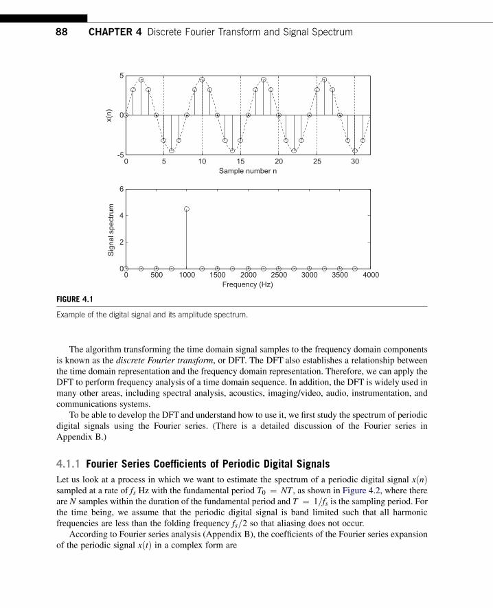
4.1 DISCRETE FOURIER TRANSFORMIn the time domain, representation of digital signals describes the signal amplitude versus the samplingtime instant or the sample number. However, in some applications, signal frequency content is veryuseful in ways other than as digital signal samples. The representation of the digital signal in terms ofits frequency component in a frequency domain, that is, the signal spectrum, needs to be developed. Asan example, Figure 4.1 illustrates the time domain representation of a 1,000-Hz sinusoid with 32samples at a sampling rate of 8,000 Hz; the bottom plot shows the signal spectrum (frequency domainrepresentation), where we can clearly observe that the amplitude peak is located at the frequency of1,000 Hz in the calculated spectrum. Hence, the spectral plot better displays the frequency informationof a digital signal.

CHAPTER

Digital Signal Processing. http://dx.doi.org/10.1016/B978-0-12-415893-1.00004-4

Copyright � 2013 Elsevier Inc. All rights reserved.87

http://dx.doi.org/10.1016/B978-0-12-415893-1.00004-4

The algorithm transforming the time domain signal samples to the frequency domain componentsis known as the discrete Fourier transform, or DFT. The DFT also establishes a relationship betweenthe time domain representation and the frequency domain representation. Therefore, we can apply theDFT to perform frequency analysis of a time domain sequence. In addition, the DFT is widely used inmany other areas, including spectral analysis, acoustics, imaging/video, audio, instrumentation, andcommunications systems.

To be able to develop the DFT and understand how to use it, we first study the spectrum of periodicdigital signals using the Fourier series. (There is a detailed discussion of the Fourier series inAppendix B.)

4.1.1 Fourier Series Coefficients of Periodic Digital Signals

Let us look at a process in which we want to estimate the spectrum of a periodic digital signal xðnÞsampled at a rate of fs Hz with the fundamental period T0 ¼ NT , as shown in Figure 4.2, where thereare N samples within the duration of the fundamental period and T ¼ 1=fs is the sampling period. Forthe time being, we assume that the periodic digital signal is band limited such that all harmonicfrequencies are less than the folding frequency fs=2 so that aliasing does not occur.

According to Fourier series analysis (Appendix B), the coefficients of the Fourier series expansionof the periodic signal xðtÞ in a complex form are

0 5 10 15 20 25 30-5

0

5

Sample number n

x(n)

0 500 1000 1500 2000 2500 3000 3500 40000

2

4

6

Frequency (Hz)

Sign

al s

pect

rum

FIGURE 4.1

Example of the digital signal and its amplitude spectrum.

88 CHAPTER 4 Discrete Fourier Transform and Signal Spectrum

ck ¼ 1

T0

ZT0

xðtÞe�jku0tdt �N < k < N (4.1)

where k is the number of harmonics corresponding to the harmonic frequency of kf0 and u0 ¼ 2p=T0and f0 ¼ 1=T0 are the fundamental frequency in radians per second and the fundamental frequency inHz, respectively. To apply Equation (4.1), we substitute T0 ¼ NT , u0 ¼ 2p=T0 and approximate theintegration over one period using a summation by substituting dt ¼ T and t ¼ nT . We obtain

ck ¼ 1

N

XN�1

n¼ 0

xðnÞe�j 2pknN ; �N < k < N (4.2)

Since the coefficients ck are obtained from the Fourier series expansion in the complex form, theresultant spectrum ck will have two sides. There is an important feature of Equation (4.2) in which theFourier series coefficient ck is periodic of N. We can verify this as follows:

ckþN ¼ 1

N

XN�1

n¼ 0

xðnÞe�j2pðkþNÞnN ¼ 1

N

XN�1

n¼ 0

xðnÞe�j2pknN e�j2pn (4.3)

Since e�j2pn ¼ cosð2pnÞ � jsinð2pnÞ ¼ 1, it follows that

ckþN ¼ ck (4.4)

Therefore, the two-side line amplitude spectrum jckj is periodic, as shown in Figure 4.3.

( )x n

n

0T NT

0

x( )0

x( )1

( ) (0)x N x

( 1) (1)x N x

N

FIGURE 4.2

Periodic digital signal.

f

kc DC component kfo = 0xfo = 0 Hz

= 2xfo = 2fo Hz

Other harmonics ...Other harmonics ...

Hz

f 0

fs – f0

fs = Nf0

fs fs + f0 f0 –fs / 2 fs / 2 –f0

2nd harmonic kfo

1st harmonic kfo = 1xfo = fo Hz

FIGURE 4.3

Amplitude spectrum of the periodic digital signal.

4.1 Discrete Fourier Transform 89

We note the following points:

a. As displayed in Figure 4.3, only the line spectral portion between the frequency �fs=2 andfrequency fs=2 (folding frequency) represents frequency information of the periodic signal.

b. Notice that the spectral portion from fs=2 to fs is a copy of the spectrum in the negative frequencyrange from�fs=2 to 0 Hz due to the spectrum being periodic for every Nf0 Hz. Again, the amplitudespectral components indexed from fs=2 to fs can be folded at the folding frequency fs=2 to match theamplitude spectral components indexed from 0 to fs=2 in terms of fs � f Hz, where f is in the rangefrom fs=2 to fs. For convenience, we compute the spectrum over the range from 0 to fs Hz withnonnegative indices, that is,

ck ¼ 1

N

XN�1

n¼ 0

xðnÞe�j2pknN ; k ¼ 0; 1;/;N � 1 (4.5)

We can apply Equation (4.4) to find the negative indexed spectral values if they are required.c. For the kth harmonic, the frequency is

f ¼ kf0 Hz (4.6)

The frequency spacing between the consecutive spectral lines, called the frequency resolution, is f0 Hz.

EXAMPLE 4.1The periodic signal

xðtÞ ¼ sinð2ptÞ

is sampled using the sampling rate fs ¼ 4 Hz.

a. Compute the spectrum ck using the samples in one period.b. Plot the two-sided amplitude spectrum jck j over the range from �2 to 2 Hz.

Solution:a. From the analog signal, we can determine the fundamental frequency u0 ¼ 2p radians per second and

f0 ¼ u0

2p¼ 2p

2p¼ 1 Hz, and the fundamental period T0 ¼ 1 second.

Since using the sampling interval T ¼ 1=fs ¼ 0:25 second, we get the sampled signal as

xðnÞ ¼ xðnT Þ ¼ sinð2pnT Þ ¼ sinð0:5pnÞ

and plot the first eight samples as shown in Figure 4.4.

x n( )

n

4N

0

1

x( )0

x( )1

x( )2

x( )3

FIGURE 4.4

Periodic digital signal.


Choosing the duration of one period, N ¼ 4, we have the following sample values:

xð0Þ ¼ 0; xð1Þ ¼ 1; xð2Þ ¼ 0; and xð3Þ ¼ �1

Using Equation (4.5),

c0 ¼ 1

4

X3n¼0

xðnÞ ¼ 1

4

�xð0Þ þ xð1Þ þ xð2Þ þ xð3Þ

�¼ 1

4ð0þ 1þ 0� 1Þ ¼ 0

c1 ¼ 1

4

X3n¼0

xðnÞe�j2p�1n=4 ¼ 1

4

�xð0Þ þ xð1Þe�jp=2 þ xð2Þe�jp þ xð3Þe�j3p=2

�

¼ 1

4

�xð0Þ � jxð1Þ � xð2Þ þ jxð3Þ ¼ 0� jð1Þ � 0þ jð�1Þ

�¼ �j0:5

Similarly, we get

c2 ¼ 1

4

X3k ¼0

xðnÞe�j2p�2n=4 ¼ 0; and c3 ¼ 1

4

X3n¼0

xðkÞe�j2p�3n=4 ¼ j0:5

Using periodicity, it follows that

c�1 ¼ c3 ¼ j0:5; and c�2 ¼ c2 ¼ 0

b. The amplitude spectrum for the digital signal is sketched in Figure 4.5.

As we know, the spectrum in the range of�2 to 2 Hz presents the information of the sinusoid with a frequencyof 1 Hz and a peak value of 2j:c1j: ¼ 1, which is obtained from converting two sides to one side by doubling thetwo-sided spectral value. Note that we do not double the direct-current (DC) component, that is, c0.

4.1.2 Discrete Fourier Transform Formulas

Now let us concentrate on development of the DFT. Figure 4.6 shows one way to obtain the DFTformula.

f11

/ 2 2sf

4sf

kc

3

4

5Hz

2345

2

0

05. 05. 05.05.05. 05.

FIGURE 4.5

Two-sided spectrum for the periodic digital signal in Example 4.1.


First, we assume that the process acquires data samples from digitizing the relevant continuoussignal for T0 seconds. Next, we assume that a periodic signal xðnÞ is obtained by cascading theacquired N data samples with the duration of T0 repetitively. Note that we assume continuity betweenthe N data sample frames. This is not true in practice. We will tackle this problem in Section 4.3.Finally, we determine the Fourier series coefficients using one-period N data samples and Equation(4.5). Then we multiply the Fourier series coefficients by a factor of N to obtain

XðkÞ ¼ Nck ¼XN�1

n¼ 0

xðnÞe�j2pknN ; k ¼ 0; 1;/;N � 1

where XðkÞ constitutes the DFT coefficients. Notice that the factor of N is a constant and does notaffect the relative magnitudes of the DFT coefficients XðkÞ. As shown in the last plot, applying DFTwith N data samples of xðnÞ sampled at a sampling rate of fs (sampling period is T ¼ 1=fs) producesN complex DFT coefficients XðkÞ. The index n is the time index representing the sample number ofthe digital sequence, whereas k is the frequency index indicating each calculated DFT coefficient,and can be further mapped to the corresponding signal frequency in terms of Hz.

Now let us conclude the DFT definition. Given a sequence xðnÞ,0� n� N � 1, its DFT is defined as

XðkÞ ¼XN�1

n¼ 0

xðnÞe�j2pkn=N ¼XN�1

n¼ 0

xðnÞWknN ; for k ¼ 0; 1;/;N � 1 (4.7)

FIGURE 4.6

Development of DFT formula.


Equation (4.7) can be expanded as

XðkÞ ¼ xð0ÞWk0N þ xð1ÞWk1

N þ xð2ÞWk2N þ/þ xðN � 1ÞWkðN�1Þ

N ; for k ¼ 0; 1;/;N � 1 (4.8)

where the factor WN (called the twiddle factor in some textbooks) is defined as

WN ¼ e�j2p=N ¼ cos

�2p

N

�� jsin

�2p

N

�(4.9)

The inverse of the DFT is given by

xðnÞ ¼ 1

N

XN�1

k¼ 0

XðkÞej2pkn=N ¼ 1

N

XN�1

k¼ 0

XðkÞW�knN ; for n ¼ 0; 1;/;N � 1 (4.10)

Proof can be found in Ahmed and Nataranjan (1983); Proakis and Manolakis (1996); Oppenheim,Schafer, and Buck (1997); and Stearns and Hush (1990).

Similar to Equation (4.7), the expansion of Equation (4.10) leads to

xðnÞ ¼ 1

N

�Xð0ÞW�0n

N þ Xð1ÞW�1nN þ Xð2ÞW�2n

N þ/þ XðN � 1ÞW�ðN�1ÞnN

�;

for n ¼ 0; 1;/;N � 1 (4.11)

As shown in Figure 4.6, in time domainwe use the sample number or time index n for indexing the digitalsample sequence xðnÞ. However, in the frequency domain, we use index k for indexingN calculatedDFTcoefficients XðkÞ. We also refer to k as the frequency bin number in Equations (4.7) and (4.8).We can use MATLAB functions fft() and ifft() to compute the DFT coefficients and the inverse DFTwith the syntax listed in Table 4.1.

The following examples serve to illustrate the application of DFT and the inverse DFT.

EXAMPLE 4.2Given a sequence xðnÞ for 0� n � 3, where xð0Þ ¼ 1, xð1Þ ¼ 2, xð2Þ ¼ 3, and xð3Þ ¼ 4, evaluate its DFT X ðkÞ.Solution:Since N ¼ 4 and W4 ¼ e�jp

2, using Equation (4.7) we have a simplified formula,

X ðkÞ ¼X3n¼0

xðnÞWkn4 ¼

X3n¼0

xðnÞe�jpkn2

Table 4.1 MATLAB FFT Functions

X ¼ fft(x) % Calculate DFT coefficients

x ¼ ifft(X) % Inverse of DFT

x ¼ input vector

X ¼ DFT coefficient vector


Thus, for k ¼ 0

X ð0Þ ¼X3n¼0

xðnÞe�j0 ¼ xð0Þe�j0 þ xð1Þe�j0 þ xð2Þe�j0 þ xð3Þe�j0

¼ xð0Þ þ xð1Þ þ xð2Þ þ xð3Þ¼ 1þ 2þ 3þ 4 ¼ 10

for k ¼ 1

X ð1Þ ¼X3n¼0

xðnÞe�jpn2 ¼ xð0Þe�j0 þ xð1Þe�jp

2 þ xð2Þe�jp þ xð3Þe�j3p2

¼ xð0Þ � jxð1Þ � xð2Þ þ jxð3Þ¼ 1� j2� 3þ j4 ¼ �2þ j2

for k ¼ 2

X ð2Þ ¼X3n¼0

xðnÞe�jpn ¼ xð0Þe�j0 þ xð1Þe�jp þ xð2Þe�j2p þ xð3Þe�j3p

¼ xð0Þ � xð1Þ þ xð2Þ � xð3Þ¼ 1� 2þ 3� 4 ¼ �2

and for k ¼ 3

X ð3Þ ¼X3n¼0

xðnÞe�j3pn2 ¼ xð0Þe�j0 þ xð1Þe�j3p

2 þ xð2Þe�j3p þ xð3Þe�j9p2

¼ xð0Þ þ jxð1Þ � xð2Þ � jxð3Þ¼ 1þ j2� 3� j4 ¼ �2� j2

Let us verify the result using the MATLAB function fft():

>> X ¼ fft([1 2 3 4 ])X ¼ 10.0000 �2.0000 þ 2.0000i �2.0000 �2.0000 �2.0000i

EXAMPLE 4.3Using the DFT coefficients X ðkÞ for 0� k � 3 computed in Example 4.2, evaluate the inverse DFT to determine thetime domain sequence xðnÞ.Solution:Since N ¼ 4 and W�1

4 ¼ ejp2, using Equation (4.10) we achieve a simplified formula,

xðnÞ ¼ 1

4

X3k¼0

X ðkÞW�nk4 ¼ 1

4

X3k¼0

X ðkÞejpkn2Then for n ¼ 0

xð0Þ ¼ 1

4

X3k ¼0

X ðkÞej0 ¼ 1

4

�X ð0Þej0 þ X ð1Þej0 þ X ð2Þej0 þ X ð3Þej0

�

¼ 1

4ð10þ ð�2þ j2Þ � 2þ ð�2� j2ÞÞ ¼ 1


for n ¼ 1

xð1Þ ¼ 1

4

X3k ¼0

X ðkÞejkp2 ¼ 1

4

�X ð0Þej0 þ X ð1Þejp2 þ X ð2Þejp þ X ð3Þej3p2

�

¼ 1

4ðX ð0Þ þ jX ð1Þ � X ð2Þ � jX ð3ÞÞ

¼ 1

4ð10þ jð�2þ j2Þ � ð�2Þ � jð�2� j2ÞÞ ¼ 2

for n ¼ 2

xð2Þ ¼ 1

4

X3k ¼0

X ðkÞejkp ¼ 1

4

�X ð0Þej0 þ X ð1Þejp þ X ð2Þej2p þ X ð3Þej3p

�

¼ 1

4ðX ð0Þ � X ð1Þ þ X ð2Þ � X ð3ÞÞ

¼ 1

4ð10� ð�2þ j2Þ þ ð�2Þ � ð�2� j2ÞÞ ¼ 3

and for n ¼ 3

xð3Þ ¼ 1

4

X3k ¼0

X ðkÞejkp32 ¼ 1

4

�X ð0Þej0 þ X ð1Þej3p2 þ X ð2Þej3p þ X ð3Þej9p2

�

¼ 1

4ðX ð0Þ � jX ð1Þ � X ð2Þ þ jX ð3ÞÞ

¼ 1

4ð10� jð�2þ j2Þ � ð�2Þ þ jð�2� j2ÞÞ ¼ 4

This example actually verifies the inverse DFT. Applying the MATLAB function ifft() we obtain

>> x ¼ ifft([10 �2þ2j �2 �2 �2j])x ¼ 1 2 3 4

Now we explore the relationship between the frequency bin k and its associated frequency.Omitting the proof, the calculated N DFT coefficients XðkÞ represent the frequency componentsranging from 0 Hz (or radians/second) to fs Hz (or us radians/second), hence we can map the frequencybin k to its corresponding frequency as follows:

u ¼ kus

Nðradians per secondÞ (4.12)

or in terms of Hz,

f ¼ kfsN

ðHzÞ (4.13)

where us ¼ 2pfs.


We can define the frequency resolution as the frequency step between two consecutive DFTcoefficients to measure how fine the frequency domain presentation is and obtain

Du ¼ us

Nðradians per secondÞ (4.14)

or in terms of Hz, it follows that

Df ¼ fsN

ðHzÞ (4.15)

Let us study the following example.

EXAMPLE 4.4

In Example 4.2, given a sequence xðnÞ for 0 � n � 3, where xð0Þ ¼ 1, xð1Þ ¼ 2, xð2Þ ¼ 3, and xð3Þ ¼ 4, wecomputed 4 DFT coefficients X ðkÞ for 0 � k � 3 as X ð0Þ ¼ 10, X ð1Þ ¼ �2þ j2, X ð2Þ ¼ �2, andX ð3Þ ¼ �2� j2. If the sampling rate is 10 Hz,

a. determine the sampling period, time index, and sampling time instant for a digital sample xð3Þ in the timedomain;

b. determine the frequency resolution, frequency bin, and mapped frequencies for the DFT coefficients X ð1Þ andX ð3Þ in the frequency domain.

Solution:a. In the time domain, the sampling period is calculated as

T ¼ 1=fs ¼ 1=10 ¼ 0:1 second

For xð3Þ, the time index is n ¼ 3 and the sampling time instant is determined by

t ¼ nT ¼ 3$0:1 ¼ 0:3 second

b. In the frequency domain, since the total number of DFT coefficients is four, the frequency resolution isdetermined by

Df ¼ fsN

¼ 10

4¼ 2:5 Hz

The frequency bin for X ð1Þ should be k ¼ 1 and its corresponding frequency is determined by

f ¼ kfsN

¼ 1� 10

4¼ 2:5 Hz

Similarly, for X ð3Þ and k ¼ 3,

f ¼ kfsN

¼ 3� 10

4¼ 7:5 Hz

Note that from Equation (4.4), k ¼ 3 is equivalent to k � N ¼ 3� 4 ¼ �1; and f ¼ 7.5 Hz is also equivalent tothe frequency f ¼ ð�1� 10Þ=4 ¼ �2:5 Hz, which corresponds to the negative side spectrum. The amplitudespectrum at 7.5 Hz after folding should match the one at fs � f ¼ 10:0� 7:5 ¼ 2:5 Hz. We will apply thesedeveloped notations in the next section for amplitude and power spectral estimation.


4.2 AMPLITUDE SPECTRUM AND POWER SPECTRUMOne DFT application is transformation of a finite-length digital signal xðnÞ into the spectrum inthe frequency domain. Figure 4.7 demonstrates such an application, where Ak and Pk arethe computed amplitude spectrum and the power spectrum, respectively, using the DFT coeffi-cients XðkÞ.

First, we obtain the digital sequence xðnÞ by sampling the analog signal xðtÞ and truncating thesampled signal with a data window of length T0 ¼ NT , where T is the sampling period and N thenumber of data points. The time for the data window is

T0 ¼ NT (4.16)

For the truncated sequence xðnÞ with a range of n ¼ 0; 1; 2;/;N � 1, we get

xð0Þ; xð1Þ; xð2Þ; .; xðN � 1Þ (4.17)

Next, we apply the DFT to the obtained sequence, xðnÞ, to get the N DFT coefficients

XðkÞ ¼XN�1

n¼ 0

xðnÞWnkN ; for k ¼ 0; 1; 2;/;N � 1 (4.18)

Since each calculated DFT coefficient is a complex number, it is not convenient to plot it versusits frequency index. Hence, after evaluating Equation (4.18), the magnitude and phase ofeach DFT coefficient (we refer to them as the amplitude spectrum and phase spectrum,respectively) can be determined and plotted versus its frequency index. We define the amplitudespectrum as

Ak ¼ 1

NjXðkÞj ¼ 1

N

ffiffiffiffiffiffiffiffiffiffiffiffiffiffiffiffiffiffiffiffiffiffiffiffiffiffiffiffiffiffiffiffiffiffiffiffiffiffiffiffiffiffiffiffiffiffiffiffiffiffiffiffiffiffiffiffiffiffiffiffiðReal½XðkÞ�Þ2 þ ðImag½XðkÞ�Þ2

q; k ¼ 0; 1; 2;/;N � 1 (4.19)

DSPprocessingDFT or FFT

Powerspectrum oramplitudespectrumx n( )

X k( )

x n( )

nT

T NT0

N 1

k

N f

N 1

A Pk k or

0

0

T fs1/

f f Ns /

N / 2

f kf Ns /

FIGURE 4.7

Applications of DFT/FFT.

4.2 Amplitude Spectrum and Power Spectrum 97

We can modify the amplitude spectrum to a one-side amplitude spectrum by doubling the amplitudesin Equation (4.19), keeping the original DC term at k ¼ 0. Thus we have

Ak ¼

8>>><>>>:

1

NjXð0Þj; k ¼ 0

2

NjXðkÞj; k ¼ 1;/;N=2

(4.20)

We can also map the frequency bin k to its corresponding frequency as

f ¼ kfsN

(4.21)

Correspondingly, the phase spectrum is given by

fk ¼ tan�1

�Imag½XðkÞ�Real½XðkÞ�

�; k ¼ 0; 1; 2;/;N � 1 (4.22)

Besides the amplitude spectrum, the power spectrum is also used. The DFT power spectrum isdefined as

Pk ¼ 1

N2jXðkÞj2¼ 1

N2

nðReal½XðkÞ�Þ2þðImag½XðkÞ�Þ2

o; k ¼ 0; 1; 2;/;N � 1 (4.23)

Similarly, for a one-sided power spectrum, we get

Pk ¼

8>>><>>>:

1

N2jXð0Þj2 k ¼ 0

2

N2jXðkÞj2 k ¼ 0; 1;/;N=2

(4.24)

and

f ¼ kfsN

(4.25)

Again, notice that the frequency resolution, which denotes the frequency spacing between DFTcoefficients in the frequency domain, is defined as

Df ¼ fsN

ðHzÞ (4.26)

It follows that better frequency resolution can be achieved by using a longer data sequence.


EXAMPLE 4.5Consider the sequence in Figure 4.8. Assuming that fs ¼ 100 Hz, compute the amplitude spectrum, phasespectrum, and power spectrum.

Solution:Since N ¼ 4, and using the DFT shown in Example 4.1, we find the DFT coefficients to be

X ð0Þ ¼ 10X ð1Þ ¼ �2þ j2X ð2Þ ¼ �2X ð3Þ ¼ �2� j2

The amplitude spectrum, phase spectrum, and power density spectrum are computed as follows:for k ¼ 0, f ¼ k$fs=N ¼ 0� 100=4 ¼ 0 Hz,

A0 ¼ 1

4jX ð0Þj ¼ 2:5; f0 ¼ tan�1

�Imag½X ð0Þ�Realð½X ð0Þ�

�¼ 00; P0 ¼ 1

42jX ð0Þj2 ¼ 6:25

for k ¼ 1, f ¼ 1� 100=4 ¼ 25 Hz,

A1 ¼ 1

4jX ð1Þj ¼ 0:7071; f1 ¼ tan�1

�Imag½X ð1Þ�Real½X ð1Þ�

�¼ 1350; P1 ¼ 1

42jX ð1Þj2 ¼ 0:5000

for k ¼ 2, f ¼ 2� 100=4 ¼ 50 Hz,

A2 ¼ 1

4jX ð2Þj ¼ 0:5; f2 ¼ tan�1


�¼ 1800; P2 ¼ 1

42jX ð2Þj2 ¼ 0:2500

Similarly,for k ¼ 3, f ¼ 3� 100=4 ¼ 75 Hz,

A3 ¼ 1

4jX ð3Þj ¼ 0:7071; f3 ¼ tan�1


�¼ �1350; P3 ¼ 1

42jX ð3Þj2 ¼ 0:5000:

Thus, the sketches for the amplitude spectrum, phase spectrum, and power spectrum are given in Figures 4.9Aand B.

x n( )

0 1 2 3

1

2

n

2

1

4 5

34

4

3

2

T NT0

FIGURE 4.8

Sampled values in Example 4.5.


Note that the folding frequency in this example is 50 Hz and the amplitude and power spectrum values at75 Hz are each image counterparts (corresponding negative-indexed frequency components), respectively. Thusvalues at 0, 25, 50 Hz correspond to the positive-indexed frequency components.

We can easily find the one-sided amplitude spectrum and one-sided power spectrum as

A0 ¼ 2:5; A1 ¼ 1:4141; A2 ¼ 1 and

P0 ¼ 6:25; P1 ¼ 2; P2 ¼ 1

FIGURE 4.9A

Amplitude spectrum and phase spectrum in Example 4.5.

FIGURE 4.9B

Power density spectrum in Example 4.5.


We plot the one-sided amplitude spectrum for comparison in Figure 4.10.Note that in the one-sided amplitude spectrum, the negative-indexed frequency components are added back

to the corresponding positive-indexed frequency components; thus each amplitude value other than the DC term isdoubled. It represents the frequency components up to the folding frequency.

EXAMPLE 4.6Consider a digital sequence sampled at the rate of 10 kHz. If we use 1,024 data points and apply the 1,024-pointDFT to compute the spectrum,

a. determine the frequency resolution;b. determine the highest frequency in the spectrum.

Solution:

a. Df ¼ fsN

¼ 10000

1024¼ 9:776 Hz

b. The highest frequency is the folding frequency, given by

fmax ¼ N

2Df ¼ fs

2

¼ 512$9:776 ¼ 5000 Hz:

As shown in Figure 4.7, the DFT coefficients may be computed via a fast Fourier transform (FFT)algorithm. The FFT is a very efficient algorithm for computing DFT coefficients. The FFT algorithmrequires a time domain sequence xðnÞwhere the number of data points is equal to a power of 2; that is,2m samples, where m is a positive integer. For example, the number of samples in xðnÞ can beN ¼ 2; 4; 8; 16; etc.

When using the FFT algorithm to compute DFT coefficients, where the length of the available datais not equal to a power of 2 (as required by the FFT), we can pad the data sequence with zeros to create

Ak

k0 1 2

2

4

f Hz( )

2 5.14141.

1

0 25 50

FIGURE 4.10

One-sided amplitude spectrum in Example 4.5.


a new sequence with a larger number of samples, N ¼ 2m > N. The modified data sequence forapplying FFT, therefore, is

xðnÞ ¼(xðnÞ 0 � n � N � 1

0 N � n � N � 1(4.27)

It is very important to note that the signal spectra obtained via zero-padding the data sequence inEquation (4.27) do not add any new information and do not contain more accurate signal spectralpresentation. In this situation, the frequency spacing is reduced due to more DFT points, and theachieved spectrum is an interpolated version with “better display.” We illustrate the zero-paddingeffect via the following example instead of theoretical analysis. A theoretical discussion of zeropadding in FFT can be found in Proakis and Manolakis (1996).

Figure 4.11(a) shows the 12 data samples from an analog signal containing frequencies of 10 Hzand 25 Hz at a sampling rate of 100 Hz, and the amplitude spectrum obtained by applying the DFT.Figure 4.11(b) displays the signal samples with padding of four zeros to the original data to make upa data sequence of 16 samples, along with the amplitude spectrum calculated by FFT. The datasequence padded with 20 zeros and its calculated amplitude spectrum using FFT are shown inFigure 4.11(c). It is evident that increasing the data length via zero padding to compute the signalspectrum does not add basic information and does not change the spectral shape but gives the

0 5 10-2

0

2

Number of samples

Orig

inal

dat

a

0 50 1000

0.5

Frequency (Hz)

Ampl

itude

spe

ctru

m

0 5 10 15-2

0

2

Number of samples

Pad

ding

4 z

eros

0 50 1000

0.5

Frequency (Hz)

Ampl

tude

spe

ctru

m

0 10 20 30-2

0

2

Number of samples

Pad

ding

20

zero

s

0 50 1000

0.5

Frequency (Hz)

Ampl

tude

spe

ctru

m

zero padding

zero padding

(a)

(b)

(c)

FIGURE 4.11

Zero-padding effect by using FFT.


“interpolated spectrum” with reduced frequency spacing. We can get a better view of the two spectralpeaks described in this case.

The only way to obtain the detailed signal spectrum with a fine frequency resolution is to applymore available data samples, that is, a longer sequence of data. Here, we choose to pad the leastnumber of zeros to satisfy the minimum FFT computational requirement. Let us look at anotherexample.

EXAMPLE 4.7We use the DFT to compute the amplitude spectrum of a sampled data sequence with a sampling ratefs ¼ 10 kHz. Given a requirement that the frequency resolution be less than 0.5 Hz, determine the number of datapoints by using the FFT algorithm, assuming that the data samples are available.

Solution:

Df ¼ 0:5 Hz

N ¼ fsDf

¼ 10;000

0:5¼ 20;000

Since we use the FFT to compute the spectrum, the number of data points must be a power of 2, that is,

N ¼ 215 ¼ 32;768

The resulting frequency resolution can be recalculated as

Df ¼ fsN

¼ 10;000

32;768¼ 0:31 Hz:

Next, we study a MATLAB example.

EXAMPLE 4.8Consider the sinusoid

xðnÞ ¼ 2$sin

�2;000p

n

8;000

�

obtained by sampling the analog signal

xðtÞ ¼ 2$sinð2;000ptÞ

with a sampling rate of fs ¼ 8,000 Hz,

a. Use the MATLAB DFT to compute the signal spectrum where the frequency resolution is equal to or lessthan 8 Hz.

b. Use the MATALB FFT and zero padding to compute the signal spectrum, assuming that the data samples in(a) are available.


Solution:a. The number of data points is

N ¼ fsDf

¼ 8;000

8¼ 1;000

There is no zero padding needed if we use the DFT formula. The detailed implementation is given in Program 4.1.The first and second plots in Figure 4.12 show the two-sided amplitude and power spectra, respectively, using theDFT, where each frequency counterpart at 7,000 Hz appears. The third and fourth plots are the one-sidedamplitude and power spectra, where the true frequency contents are displayed from 0 Hz to the Nyquist frequencyof 4 kHz (folding frequency).b. If the FFT is used, the number of data points must be a power of 2. Hence we choose

N ¼ 210 ¼ 1;024

Assuming there are only 1,000 data samples available in (a), we need to pad 24 zeros to the original 1,000data samples before applying the FFT algorithm, as required. Thus the calculated frequency resolution isDf ¼ fs=N ¼ 8;000=1;024 ¼ 7:8125 Hz. Note that this is an interpolated frequency resolution by using zeropadding. The zero padding actually interpolates a signal spectrum and carries no additional frequency information.Figure 4.13 shows the spectral plots using FFT. The detailed implementation is given in Program 4.1.Program 4.1. MATLAB program for Example 4.8.

% Example 4.8close all;clear all% Generate the sine wave sequencefs¼8000; % Sampling rateN¼1000; % Number of data pointsx¼2*sin(2000*pi*[0:1:N-1]/fs);% Apply the DFT algorithmfigure(1)xf¼abs(fft(x))/N; % Compute the amplitude spectrumP¼xf.*xf; % Compute power spectrumf¼[0:1:N-1]*fs/N; % Map the frequency bin to frequency (Hz)subplot(2,1,1); plot(f,xf);gridxlabel(’Frequency (Hz)’); ylabel(’Amplitude spectrum (DFT)’);subplot(2,1,2);plot(f,P);gridxlabel(’Frequency (Hz)’); ylabel(’Power spectrum (DFT)’);figure(2)% Convert it to one side spectrumxf(2:N)¼2*xf(2:N); % Get the single-side spectrumP¼xf.*xf; % Calculate the power spectrumf¼[0:1:N/2]*fs/N % Frequencies up to the folding frequencysubplot(2,1,1); plot(f,xf(1:N/2þ1));gridxlabel(’Frequency (Hz)’); ylabel(’Amplitude spectrum (DFT)’);subplot(2,1,2);plot(f,P(1:N/2þ1));gridxlabel(’Frequency (Hz)’); ylabel(’Power spectrum (DFT)’);figure (3)% Zero padding to the length of 1024x¼[x,zeros(1,23)];N¼length(x);xf¼abs(fft(x))/N; % Compute amplitude spectrum with zero paddingP¼xf.*xf; % Compute power spectrumf¼[0:1:N-1]*fs/N; % Map frequency bin to frequency (Hz)subplot(2,1,1); plot(f,xf);grid


0 1000 2000 3000 4000 5000 6000 7000 80000

0.5

1

Frequency (Hz)

Ampl

itude

spe

ctru

m (D

FT)

0 1000 2000 3000 4000 5000 6000 7000 80000

0.2

0.4

0.6

0.8

1

Frequency (Hz)

Pow

er s

pect

rum

(DFT

)

0 500 1000 1500 2000 2500 3000 3500 40000

0.5

1

1.5

2

Frequency (Hz)

Ampl

itude

spe

ctru

m (D

FT)

0 500 1000 1500 2000 2500 3000 3500 40000

1

2

3

4

Frequency (Hz)

Pow

er s

pect

rum

(DFT

)

FIGURE 4.12

Amplitude spectrum and power spectrum using DFT for Example 4.8.


0 1000 2000 3000 4000 5000 6000 7000 80000

0.5

1

Frequency (Hz)

Ampl

itude

spe

ctru

m (F

FT)

0 1000 2000 3000 4000 5000 6000 7000 80000

0.2

0.4

0.6

0.8

1

Frequency (Hz)

Pow

er s

pect

rum

(FFT

)

0 500 1000 1500 2000 2500 3000 3500 40000

0.5

1

1.5

2

Frequency (Hz)

Ampl

itude

spe

ctru

m (F

FT)

0 500 1000 1500 2000 2500 3000 3500 40000

1

2

3

4

Frequency (Hz)

Pow

er s

pect

rum

(FFT

)

FIGURE 4.13

Amplitude spectrum and power spectrum using FFT for Example 4.8.


xlabel(’Frequency (Hz)’); ylabel(’Amplitude spectrum (FFT)’);subplot(2,1,2);plot(f,P);gridxlabel(’Frequency (Hz)’); ylabel(’Power spectrum (FFT)’);figure(4)% Convert it to one side spectrumxf(2:N)¼2*xf(2:N);P¼xf.*xf;f¼[0:1:N/2]*fs/N;subplot(2,1,1); plot(f,xf(1:N/2þ1));gridxlabel(’Frequency (Hz)’); ylabel(’Amplitude spectrum (FFT)’);subplot(2,1,2);plot(f,P(1:N/2þ1));gridxlabel(’Frequency (Hz)’); ylabel(’Power spectrum (FFT)’);

4.3 SPECTRAL ESTIMATION USING WINDOW FUNCTIONSWhen we apply DFT to the sampled data in the previous section, we theoretically imply the followingassumptions: first, that the sampled data are periodic (repeat themselves), and second, that the sampleddata are continuous and band limited to the folding frequency. The second assumption is oftenviolated, and the discontinuity produces undesired harmonic frequencies. Consider a pure 1-Hz sinewave with 32 samples shown in Figure 4.14.

As shown in the figure, if we use a window size of N ¼ 16 samples, which is a multiple of the twowaveform cycles, the second window has continuity with the first. However, when the window size is

0 5 10 15 20 25 30 35-1

-0.5

0

0.5

1

x(n)

Window size: N=16 (multiple of waveform cycles)

0 5 10 15 20 25 30 35 40-1

-0.5

0

0.5

1

Window size: N=18 (not multiple of waveform cycles)

x(n)

FIGURE 4.14

Sampling a 1-Hz sine wave using (top) 16 samples per cycle and (bottom) 18 samples per cycle.

4.3 Spectral Estimation Using Window Functions 107

chosen to be 18 samples, which is not multiple of the waveform cycles (2.25 cycles), there isa discontinuity in the second window. It is this discontinuity that produces harmonic frequenciesthat are not present in the original signal. Figure 4.15 shows the spectral plots for both cases using theDFT/FFT directly.

The first spectral plot contains a single frequency, as we expected, while the second spectrum hasthe expected frequency component plus many harmonics, which do not exist in the original signal.We called such an effect spectral leakage. The amount of spectral leakage shown in the second plotis due to amplitude discontinuity in time domain. The bigger the discontinuity, the more the leakage.To reduce the effect of spectral leakage, a window function can be used whose amplitude taperssmoothly and gradually toward zero at both ends. Applying the window function wðnÞ to a datasequence xðnÞ to obtain the windowed sequence xwðnÞ is illustrated in Figure 4.16 usingEquation (4.28):

xwðnÞ ¼ xðnÞwðnÞ; for n ¼ 0; 1;/;N � 1 (4.28)

The top plot is the data sequence xðnÞ, and the middle plot is the window function wðnÞ. The bottomplot in Figure 4.16 shows that the windowed sequence xwðnÞ is tapped down by a window function tozero at both ends such that the discontinuity is dramatically reduced.

0 5 10 15-1

-0.5

0

0.5

1

x(n)

Window size: N=160 5 10 15

0

0.2

0.4

0.6

0.8

Ak

Window size: N=16

0 5 10 15-1

-0.5

0

0.5

1

x(n)

Window size:N=180 5 10 15

0

0.2

0.4

Ak

Window size: N=18

FIGURE 4.15

Signal samples and spectra without spectral leakage and with spectral leakage.


EXAMPLE 4.9In Figure 4.16, given

• xð2Þ ¼ 1 and wð2Þ ¼ 0:2265• xð5Þ ¼ �0:7071 and wð5Þ ¼ 0:7008

calculate the windowed sequence data points xw ð2Þ and xw ð5Þ.Solution:Applying the window function operation leads to

xw ð2Þ ¼ xð2Þ � wð2Þ ¼ 1� 0:2265 ¼ 0:2265 andxw ð5Þ ¼ xð5Þ � wð5Þ ¼ �0:7071� 0:7008 ¼ �0:4956

which agree with the values shown in the bottom plot in Figure 4.16.

Using the window function shown in Example 4.9, the spectral plot is reproduced. As a result, thespectral leakage is greatly reduced, as shown in Figure 4.17.

The common window functions are listed as follows.The rectangular window (no window function):

wRðnÞ ¼ 1; 0 � n � N � 1 (4.29)

0 2 4 6 8 10 12 14 16-1

0

1

x(n)

0 2 4 6 8 10 12 14 160

0.5

1

Win

dow

w(n

)

0 2 4 6 8 10 12 14 16-1

0

1

Win

dow

ed x

w(n

)

Time index n

FIGURE 4.16

Illustration of the window operation.


The triangular window:

wtriðnÞ ¼ 1� j2n� N þ 1jN � 1

; 0 � n � N � 1 (4.30)

The Hamming window:

whmðnÞ ¼ 0:54� 0:46cos

�2pn

N � 1

�; 0 � n � N � 1 (4.31)

The Hanning window:

whnðnÞ ¼ 0:5� 0:5cos

�2pn

N � 1

�; 0 � n � N � 1 (4.32)

Plots for each window function for a size of 20 samples are shown in Figure 4.18.The following example details each step for computing the spectral information using the windowfunctions.

0 5 10 15-1

-0.5

0

0.5

1

x(n)

(orig

inal

sig

nal)

Time index n0 5 10 15

0

0.2

0.4

Ak

Frequency index

0 5 10 15-1

-0.5

0

0.5

1

Win

dow

ed x

(n)

Time index n0 5 10 15

0

0.2

0.4

Win

dow

ed A

k

Frequency index

FIGURE 4.17

Comparison of spectra calculated without using a window function and using a window function to reduce

spectral leakage.


EXAMPLE 4.10Considering the sequence xð0Þ ¼ 1, xð1Þ ¼ 2, xð2Þ ¼ 3, xð3Þ ¼ 4, and given fs ¼ 100 Hz,T ¼ 0:01 seconds; compute the amplitude spectrum, phase spectrum, and power spectrum

a. using the triangle window function;b. using the Hamming window function.

Solution:a. Since N ¼ 4, from the triangular window function, we have

wtrið0Þ ¼ 1� j2� 0� 4þ 1j4� 1

¼ 0

wtrið1Þ ¼ 1� j2� 1� 4þ 1j4� 1

¼ 0:6667

Similarly, wtrið2Þ ¼ 0:6667, wtrið3Þ ¼ 0. Next, the windowed sequence is computed as

xw ð0Þ ¼ xð0Þ � wtrið0Þ ¼ 1� 0 ¼ 0xw ð1Þ ¼ xð1Þ � wtrið1Þ ¼ 2� 0:6667 ¼ 1:3334xw ð2Þ ¼ xð2Þ � wtrið2Þ ¼ 3� 0:6667 ¼ 2xw ð3Þ ¼ xð3Þ � wtrið3Þ ¼ 4� 0 ¼ 0

0 5 10 15 200

0.2

0.4

0.6

0.8

1

Rec

tang

ular

win

dow

0 5 10 15 200

0.2

0.4

0.6

0.8

1

Tria

ngul

ar w

indo

w

0 5 10 15 200

0.2

0.4

0.6

0.8

1

Ham

min

g w

indo

w

0 5 10 15 200

0.2

0.4

0.6

0.8

1

Han

ning

win

dow

FIGURE 4.18

Plots of window sequences.


Applying DFT Equation (4.8) to xw ðnÞ for k ¼ 0;1;2;3, respectively,

X ðkÞ ¼ xw ð0ÞWk�04 þ xð1ÞWk�1

4 þ xð2ÞWk�24 þ xð3ÞWk�3

4

We obtain the following results:

X ð0Þ ¼ 3:3334X ð1Þ ¼ �2� j1:3334X ð2Þ ¼ 0:6666X ð3Þ ¼ �2þ j1:3334

Df ¼ 1

NT¼ 1

4$0:01¼ 25 Hz

Applying Equations (4.19), (4.22), and (4.23) leads to

A0 ¼ 1

4jX ð0Þj ¼ 0:8334; f0 ¼ tan�1

�0

3:3334

�¼ 00; P0 ¼ 1

42jX ð0Þj2 ¼ 0:6954

A1 ¼ 1

4jX ð1Þj ¼ 0:6009; f1 ¼ tan�1

��1:3334

�2

�¼ �146:310; P1 ¼ 1

42jX ð1Þj2

¼ 0:3611

A2 ¼ 1

4jX ð2Þj ¼ 0:1667; f2 ¼ tan�1

�0

0:6666

�¼ 00; P1 ¼ 1

42jX ð2Þj2 ¼ 0:0278

Similarly,

A3 ¼ 1

4jX ð3Þj ¼ 0:6009; f3 ¼ tan�1

�1:3334

�2

�¼ 146:310; P3 ¼ 1

42jX ð3Þj2 ¼ 0:3611

b. Since N ¼ 4, from the Hamming window function, we have

whmð0Þ ¼ 0:54� 0:46 cos

�2p� 0

4� 1

�¼ 0:08

whmðnÞ ¼ 0:54� 0:46 cos

�2p� 1

4� 1

�¼ 0:77

Similarly,whmð2Þ ¼ 0:77, whmð3Þ ¼ 0:08. Next, the windowed sequence is computed as

xw ð0Þ ¼ xð0Þ � whmð0Þ ¼ 1� 0:08 ¼ 0:08xw ð1Þ ¼ xð1Þ � whmð1Þ ¼ 2� 0:77 ¼ 1:54xw ð2Þ ¼ xð2Þ � whmð2Þ ¼ 3� 0:77 ¼ 2:31xw ð0Þ ¼ xð3Þ � whmð3Þ ¼ 4� 0:08 ¼ 0:32

Applying DFT Equation (4.8) to xw ðnÞ for k ¼ 0;1;2;3, respectively,

X ðkÞ ¼ xw ð0ÞWk�04 þ xð1ÞWk�1

4 þ xð2ÞWk�24 þ xð3ÞWk�3

4


We obtain the following:

X ð0Þ ¼ 4:25X ð1Þ ¼ �2:23� j1:22X ð2Þ ¼ 0:53X ð3Þ ¼ �2:23þ j1:22

Df ¼ 1

NT¼ 1

4$0:01¼ 25 Hz

Applying Equations (4.19), (4.22), and (4.23), we achieve

A0 ¼ 1

4jX ð0Þj ¼ 1:0625; f0 ¼ tan�1

�0

4:25

�¼ 00; P0 ¼ 1

42jX ð0Þj2 ¼ 1:1289

A1 ¼ 1

4jX ð1Þj ¼ 0:6355; f1 ¼ tan�1

��1:22

�2:23

�¼ �151:320; P1 ¼ 1

42jX ð1Þj2 ¼ 0:4308

A2 ¼ 1

4jX ð2Þj ¼ 0:1325; f2 ¼ tan�1

�0

0:53

�¼ 00 ; P2 ¼ 1

42jX ð2Þj2 ¼ 0:0176

Similarly,

A3 ¼ 1

4jX ð3Þj ¼ 0:6355; f3 ¼ tan�1

�1:22

�2:23

�¼ 151:320; P3 ¼ 1

42jX ð3Þj2 ¼ 0:4308

EXAMPLE 4.11Given the sinusoid

xðnÞ ¼ 2$sin

�2;000p

n

8;000

�

obtained using a sampling rate of fs ¼ 8;000 Hz, use the DFT to compute the spectrum with the followingspecifications:

a. Compute the spectrum of a triangular window function with window size ¼ 50.b. Compute the spectrum of a Hamming window function with window size ¼ 100.c. Compute the spectrum of a Hanning window function with window size ¼ 150 and a one-sided spectrum.

Solution:The MATLAB program is listed in Program 4.2, and results are plotted in Figures 4.19 to 4.21. As compared withthe no-window (rectangular window) case, all three windows are able to effectively reduce the spectral leakage, asshown in the figures.Program 4.2. MATLAB program for Example 4.11.%Example 4.11close all;clear all% Generate the sine wave sequencefs¼8000; T¼1/fs; % Sampling rate and sampling periodx¼2*sin(2000*pi*[0:1:50]*T); % Generate 51 2000-Hz samples.% Apply the FFT algorithmN¼length(x);


index_t¼[0:1:N-1];f¼[0:1:N-1]*8000/N; % Map frequency bin to frequency (Hz)xf¼abs(fft(x))/N; % Calculate amplitude spectrumfigure(1)%Using Bartlett windowx_b¼x.*bartlett(N)’; % Apply triangular window functionxf_b¼abs(fft(x_b))/N; % Calculate amplitude spectrumsubplot(2,2,1);plot(index_t,x);gridxlabel(’Time index n’); ylabel(’x(n)’);subplot(2,2,3); plot(index_t,x_b);gridxlabel(’Time index n’); ylabel(’Triangular windowed x(n)’);subplot(2,2,2);plot(f,xf);grid;axis([0 8000 0 1]);xlabel(’Frequency (Hz)’); ylabel(’Ak (no window)’);subplot(2,2,4); plot(f,xf_b);grid; axis([0 8000 0 1]);xlabel(’Frequency (Hz)’); ylabel(’Triangular windowed Ak’);figure(2)% Generate the sine wave sequencex¼2*sin(2000*pi*[0:1:100]*T); % Generate 101 2000-Hz samples.% Apply the FFT algorithmN¼length(x);index_t¼[0:1:N-1];f¼[0:1:N-1]*fs/N;xf¼abs(fft(x))/N;% Using Hamming windowx_hm¼x.*hamming(N)’; % Apply Hamming window functionxf_hm¼abs(fft(x_hm))/N; % Calculate amplitude spectrumsubplot(2,2,1);plot(index_t,x);gridxlabel(’Time index n’); ylabel(’x(n)’);subplot(2,2,3); plot(index_t,x_hm);gridxlabel(’Time index n’); ylabel(’Hamming windowed x(n)’);subplot(2,2,2);plot(f,xf);grid;axis([0 fs 0 1]);xlabel(’Frequency (Hz)’); ylabel(’Ak (no window)’);subplot(2,2,4); plot(f,xf_hm);grid;axis([0 fs 0 1]);xlabel(’Frequency (Hz)’); ylabel(’Hamming windowed Ak’);figure(3)% Generate the sine wave sequencex¼2*sin(2000*pi*[0:1:150]*T); % Generate 151 2-kHz samples% Apply the FFT algorithmN¼length(x);index_t¼[0:1:N-1];f¼[0:1:N-1]*fs/N;xf¼2*abs(fft(x))/N;xf(1)¼xf(1)/2; % Single-sided spectrum%Using Hanning windowx_hn¼x.*hanning(N)’;xf_hn¼2*abs(fft(x_hn))/N;xf_hn(1)¼xf_hn(1)/2; % Single-sided spectrumsubplot(2,2,1);plot(index_t,x);gridxlabel(’Time index n’); ylabel(’x(n)’);subplot(2,2,3); plot(index_t,x_hn);gridxlabel(’Time index n’); ylabel(’Hanning windowed x(n)’);subplot(2,2,2);plot(f(1:(N-1)/2),xf(1:(N-1)/2));grid;axis([0 fs/2 0 1]);xlabel(’Frequency (Hz)’); ylabel(’Ak (no window)’);subplot(2,2,4); plot(f(1:(N-1)/2),xf_hn(1:(N-1)/2));grid;axis([0 fs/2 0 1]);xlabel(’Frequency (Hz)’); ylabel(’Hanning windowed Ak’);


0 20 40 60-2

-1

0

1

2

Time index n

x(n)

0 20 40 60-2

-1

0

1

2

Time index n

Tria

ngul

ar w

indo

wed

x(n

)

0 2000 4000 6000 80000

0.5

1

Frequency (Hz)

Ak (n

o w

indo

w)

0 2000 4000 6000 80000

0.2

0.4

0.6

0.8

1

Frequency (Hz)Tr

iang

ular

win

dow

ed A

k

FIGURE 4.19

Comparison of a spectrum without using a window function and a spectrum using a triangular window with

50 samples in Example 4.11.

0 50 100-2

-1

0

1

2

Time index n

x(n)

0 50 100-2

-1

0

1

2

Time index n

Ham

min

g w

indo

wed

x(n

)

0 2000 4000 6000 80000

0.5

1

Frequency (Hz)

Ak (n

o w

indo

w)

0 2000 4000 6000 80000

0.2

0.4

0.6

0.8

1

Frequency (Hz)

Ham

min

g w

indo

wed

Ak

FIGURE 4.20

Comparison of a spectrum without using a window function and a spectrum using a Hamming window with

100 samples in Example 4.11.


4.4 APPLICATION TO SIGNAL SPECTRAL ESTIMATIONThe following plots compare amplitude spectra for speech data (we.dat) with 2,001 samples anda sampling rate of 8,000 Hz using the rectangular window (no window) function and theHamming window function. As demonstrated in Figure 4.22 (two-sided spectrum) and Figure 4.23(one-sided spectrum), there is little difference between the amplitude spectrum using theHamming window function and the spectrum without using the window function. This is due tothe fact that when the data length of the sequence (e.g., 2,001 samples) increases, the frequencyresolution will be improved and the spectral leakage will become less significant. However, whendata length is short, the reduction in spectral leakage using a window function will be moreprominent.

Next, we compute the one-sided spectrum for 32-bit seismic data sampled at 15 Hz (provided bythe US Geological Survey, Albuquerque Seismological Laboratory) with 6,700 data samples. Thecomputed spectral plots without using a window function and using the Hamming window aredisplayed in Figure 4.24. We can see that most of seismic signal components are below 3 Hz.

0 50 100 150-2

-1

0

1

2

Time index n

x(n)

0 50 100 150-2

-1

0

1

2

Time index n

Han

ning

win

dow

ed x

(n)

0 1000 2000 3000 40000

0.5

1

1.5

2

Frequency (Hz)

Ak (n

o w

indo

w)

0 1000 2000 3000 40000

0.5

1

1.5

2

Frequency (Hz)

Han

ning

win

dow

ed A

k

FIGURE 4.21

Comparison of a one-sided spectrum without using the window function and a one-sided spectrum using

a Hanning window with 150 samples in Example 4.11.


0 500 1000 1500 2000-1

-0.5

0

0.5

1x 104

Time index n

x(n)

0 500 1000 1500 2000-5000

0

5000

10000

Time index n

Ham

min

g w

indo

wed

x(n

)

0 2000 4000 6000 80000

100

200

300

400

Frequency (Hz)

Ampl

itude

spe

ctru

m A

k0 2000 4000 6000 8000

0

100

200

300

400

Frequency (Hz)H

amm

ing

win

dow

ed A

k

FIGURE 4.22

Comparison of a spectrum without using a window function and a spectrum using the Hamming window for

speech data.

0 500 1000 1500 2000-1

-0.5

0

0.5

1x 104

Time index n

x(n)

0 500 1000 1500 2000-5000

0

5000

10000

Time index n

Ham

min

g w

indo

wed

x(n

)

0 1000 2000 30000

200

400

600

800

Frequency (Hz)

Ampl

itude

spe

ctru

m A

k

0 1000 2000 30000

200

400

600

800

Frequency (Hz)

Ham

min

g w

indo

wed

Ak

FIGURE 4.23

Comparison of a one-sided spectrum without using a window function and a one-sided spectrum using the

Hamming window for speech data.

4.4 Application to Signal Spectral Estimation 117

0 2000 4000 6000 8000-5

0

5x 105

Time index n

x(n)

0 2000 4000 6000 8000-4

-2

0

2

4x 105

Time index n

Ham

min

g w

indo

wed

x(n

)

0 2 4 60

2000

4000

6000

Frequency (Hz)

Ampl

itude

spe

ctru

m A

k0 2 4 6

0

2000

4000

6000

Frequency (Hz)

Ham

min

g w

indo

wed

Ak

FIGURE 4.24


Hamming window for seismic data.

0 2000 4000 6000-5000

0

5000

10000

Time index n

x(n)

0 2000 4000 6000-5000

0

5000

10000

Time index n

Ham

min

g w

indo

wed

x(n

)

0 100 2000

200

400

600

Frequency (Hz)

Ampl

itude

spe

ctru

m A

k

0 100 2000

200

400

600

Frequency (Hz)

Ham

min

g w

indo

wed

Ak

60-Hz interference

60-Hz interference

FIGURE 4.25


Hamming window for electrocardiogram data.


We also compute the one-sided spectrum for a standard electrocardiogram (ECG) signal from theMIT–BIH (Massachusetts Institute of Technology–Beth Israel Hospital) Database. The ECG signalcontains frequency components ranging from 0.05 to 100 Hz sampled at 500 Hz. As shown inFigure 4.25, there is a spike located at 60 Hz. This is due to the 60-Hz power line interference when theECG is acquired via the ADC acquisition process. This 60-Hz interference can be removed by usinga digital notch filter, which will be studied in Chapter 8.

Figure 4.26 shows a vibration signal and its spectrum. The vibration signal is captured using anaccelerometer sensor attached to a simple supported beam while an impulse force is applied toa location that is close to the middle of the beam. The sampling rate is 1 kHz. As shown in Figure 4.26,four dominant modes (natural frequencies corresponding to locations of spectral peaks) can be easilyidentified from the displayed spectrum.

We now present another practical example for vibration signature analysis of a defective geartooth, described in Section 1.3.5. Figure 4.27 shows a gearbox containing two straight bevel gearswith a transmission ratio of 1.5:1 and the number of teeth on the pinion and gear are 18 and 27.The vibration data is collected by an accelerometer installed on the top of the gearbox. Thedata acquisition system uses a sampling rate of 12.8 kHz. The meshing frequency is determined asfm ¼ fiðRPMÞ � 18=60 ¼ 300 Hz, where the input shaft frequency is fi ¼ 1000 RPM ¼ 16:67Hz.Figures 4.28–4.31 show the baseline vibration signal and spectrum for a gearbox in good condition,

0 500 1000 1500 2000

-1

-0.5

0

0.5

1

Time index n

x(n)

0 500 1000 1500 2000

-1

-0.5

0

0.5

1

Time index n

Ham

min

g w

indo

wed

x(n

)

0 100 200 300 400 5000

0.01

0.02

0.03

0.04

Frequency (Hz)

Ampl

itude

spe

ctru

m A

k

0 100 200 300 400 5000

0.01

0.02

0.03

0.04

Frequency (Hz)

Ham

min

g w

indo

wed

Ak

Components corresponding to natural frequencies

Components correspondingto natural frequencies

FIGURE 4.26


Hamming window for vibration signal.


along with the vibration signals and spectra for three different damage severity levels (there are fivelevels classified by SpectraQuest, Inc; the spectrums shown are for severity level 1 [lightly chipped];severity level 4 [heavily chipped]; and severity level 5 [missing tooth]). As we can see, the baselinespectrum contains the meshing frequency component of 300 Hz and a sideband frequency compo-nent of 283.33 Hz (300–16.67). We can observe that the sidebands (fm � fi, fm � 2fi .) becomemore dominant when the severity level increases. Hence, the spectral information is very useful formonitoring the health condition of the gearbox.

(a) Gearbox (b) Pinion and gear

(c) Damaged pinion

missing tooth

FIGURE 4.27

Vibration signature analysis of a gearbox.

(Courtesy of SpectaQuest, Inc.)


0 2 4 6 8 10 12 14-0.5

0

0.5

Time (sec.)Am

plitu

de (V

)

0 1000 2000 3000 4000 5000 6000 70000

0.01

0.02

Frequency (Hz)

Ampl

itude

(VR

MS)

250 260 270 280 290 300 310 320 330 340 3500

0.01

0.02

Zoomed Frequency (Hz)

Ampl

itude

(VR

MS)

Meshing frequency

Meshing frequencySideband frequency fm-fi

FIGURE 4.28

Vibration signal and spectrum from the good condition gearbox.

(Data provided by SpectaQuest, Inc.)

0 2 4 6 8 10 12 14-1

0

1

Time (sec.)

Ampl

itude

(V)

0 1000 2000 3000 4000 5000 6000 70000

0.01

0.02

Frequency (Hz)

Ampl

itude

(VR

MS)

250 260 270 280 290 300 310 320 330 340 3500

0.01

0.02


Ampl

itude

(VR

MS)

Meshing frequency

Meshing frequencySidebands Sidebands

FIGURE 4.29

Vibration signal and spectrum for damage severity level 1.



0 2 4 6 8 10 12 14-1

0

1

Time (sec.)Am

plitu

de (V

)

0 1000 2000 3000 4000 5000 6000 70000

0.005

0.01

Frequency (Hz)

Ampl

itude

(VR

MS)

250 260 270 280 290 300 310 320 330 340 3500

0.01

0.02


Ampl

itude

(VR

MS)

Meshing frequency

Meshing frequencySidebandsSidebands

FIGURE 4.30



0 2 4 6 8 10 12 14-2

0

2

Time (sec.)

Ampl

itude

(V)

0 1000 2000 3000 4000 5000 6000 70000

0.02

0.04

Frequency (Hz)

Ampl

itude

(VR

MS)

250 260 270 280 290 300 310 320 330 340 3500

0.01

0.02


Ampl

itude

(VR

MS)

Meshing frequency

Meshing frequencySidebandsSidebands

FIGURE 4.31




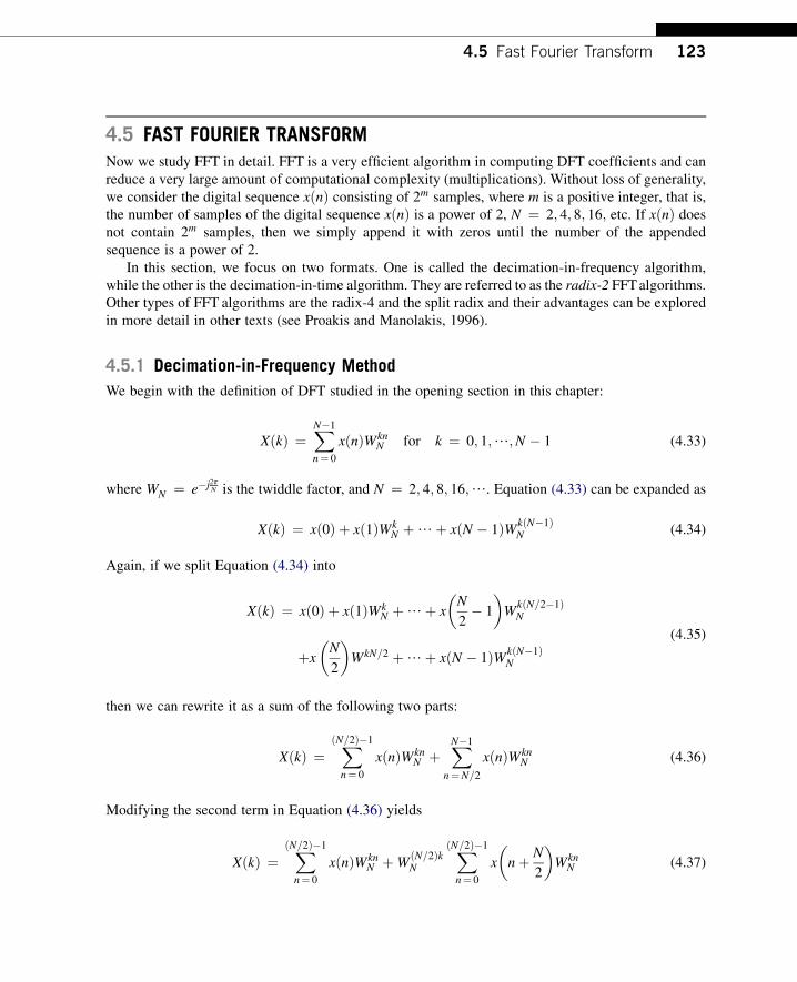
4.5 FAST FOURIER TRANSFORMNow we study FFT in detail. FFT is a very efficient algorithm in computing DFT coefficients and canreduce a very large amount of computational complexity (multiplications). Without loss of generality,we consider the digital sequence xðnÞ consisting of 2m samples, where m is a positive integer, that is,the number of samples of the digital sequence xðnÞ is a power of 2, N ¼ 2; 4; 8; 16; etc. If xðnÞ doesnot contain 2m samples, then we simply append it with zeros until the number of the appendedsequence is a power of 2.

In this section, we focus on two formats. One is called the decimation-in-frequency algorithm,while the other is the decimation-in-time algorithm. They are referred to as the radix-2 FFTalgorithms.Other types of FFT algorithms are the radix-4 and the split radix and their advantages can be exploredin more detail in other texts (see Proakis and Manolakis, 1996).

4.5.1 Decimation-in-Frequency Method

We begin with the definition of DFT studied in the opening section in this chapter:

XðkÞ ¼XN�1

n¼ 0

xðnÞWknN for k ¼ 0; 1;/;N � 1 (4.33)

where WN ¼ e�j2pN is the twiddle factor, and N ¼ 2; 4; 8; 16;/. Equation (4.33) can be expanded as

XðkÞ ¼ xð0Þ þ xð1ÞWkN þ/þ xðN � 1ÞWkðN�1Þ

N (4.34)

Again, if we split Equation (4.34) into

XðkÞ ¼ xð0Þ þ xð1ÞWkN þ/þ x

�N

2� 1

�W

kðN=2�1ÞN

þx

�N

2

�WkN=2 þ/þ xðN � 1ÞWkðN�1Þ

N

(4.35)

then we can rewrite it as a sum of the following two parts:

XðkÞ ¼XðN=2Þ�1

n¼ 0

xðnÞWknN þ

XN�1

n¼N=2

xðnÞWknN (4.36)

Modifying the second term in Equation (4.36) yields


n¼ 0

xðnÞWknN þW

ðN=2ÞkN

XðN=2Þ�1

n¼ 0

x

�nþ N

2

�Wkn

N (4.37)

4.5 Fast Fourier Transform 123

Recall WN=2N ¼ e�j2pðN=2Þ

N ¼ e�jp ¼ �1 ; then we have


n¼ 0

�xðnÞ þ ð�1Þkx

�nþ N

2

��Wkn

N (4.38)

Now letting k ¼ 2m be an even number we obtain

Xð2mÞ ¼XðN=2Þ�1

n¼ 0

�xðnÞ þ x

�nþ N

2

��W2mn

N (4.39)

while substituting k ¼ 2mþ 1 (an odd number) yields

Xð2mþ 1Þ ¼XðN=2Þ�1

n¼ 0

�xðnÞ � x

�nþ N

2

��Wn

NW2mnN (4.40)

Using the fact that W2N ¼ e�j2p�2

N ¼ e�j 2pðN=2Þ ¼ WN=2, it follows that

Xð2mÞ ¼XðN=2Þ�1

n¼ 0

aðnÞWmnN=2 ¼ DFTfaðnÞwithðN=2Þpointsg (4.41)

Xð2mþ 1Þ ¼XðN=2Þ�1

n¼ 0

bðnÞWnNW

mnN=2 ¼ DFT

�bðnÞWn

N with ðN=2Þpoints� (4.42)

where aðnÞ and bðnÞ are introduced and expressed as

aðnÞ ¼ xðnÞ þ x

�nþ N

2

�; for n ¼ 0; 1/;

N

2� 1 (4.43a)

bðnÞ ¼ xðnÞ � x

�nþ N

2

�; for n ¼ 0; 1;/;

N

2� 1 (4.43b)

Equations (4.33), (4.41), and (4.42) can be summarized as

DFTfxðnÞ with N pointsg ¼(

DFTfaðnÞ with ðN=2Þ pointsgDFT

�bðnÞWn

N with ðN=2Þ points� (4.44)

The computation process is illustrated in Figure 4.32. As shown in this figure, there are three graphicaloperations, which are illustrated Figure 4.33.If we continue the process described by Figure 4.32, we obtain the block diagrams shown in Figures4.34 and 4.35.

Figure 4.35 illustrates the FFT computation for the eight-point DFT, where there are 12 complexmultiplications. This is a big saving as compared with the eight-point DFT with 64 complex


x( )0x( )1

x( )3

x( )4

x( )5

x( )6

x( )7

x( )2

a( )0

a( )1

a( )2

a( )3

b( )0

b( )1

b( )2

b( )3

WN0

WN1

WN2

WN3

N

2- point

N

2- point

DFT

DFT

1

1

1

1

X ( )0

X ( )2X ( )4

X ( )6

X ( )1

X ( )3

X ( )5X ( )7

FIGURE 4.32

The first iteration of the eight-point FFT.

x

y

z x y

1

x

yz x y

xw

z wx

FIGURE 4.33

Definitions of the graphical operations.

x( )0x( )1

x( )3

x( )4

x( )5

x( )6

x( )7

x( )2

WN0

WN1

WN2

WN3

N

4- point

DFT

1

1

1

1

X ( )0

X ( )4X ( )2

X ( )6

X ( )1

X ( )5

X ( )3X ( )7

N

4- point

DFT

N

4- point

DFT

N

4- point

DFT

WN0

WN0

WN2

WN2

1

1

1

1

FIGURE 4.34

The second iteration of the eight-point FFT.

X ( )0

X ( )4

X ( )2

X ( )6

X ( )1

X ( )5

X ( )3

X ( )7

WN0

WN0

WN0

WN0

1

1

1

1

x( )0

x( )1

x( )3

x( )4

x( )5

x( )6

x( )7

x( )2

WN0

WN1

WN2

WN3

1

1

1

1

WN0

WN0

WN2

WN2

1

1

1

1

FIGURE 4.35

Block diagram for the eight-point FFT (total 12 multiplications).


multiplications. For a data length of N, the number of complex multiplications for DFT and FFT,respectively, are determined by

Complex multiplications of DFT ¼ N2; and

Complex multiplications of FFT ¼ N

2log2ðNÞ

To see the effectiveness of FFT, let us consider a sequence with 1,024 data points. Applying DFTwill require 1; 024� 1; 024 ¼ 1; 048; 576 complex multiplications; however, applying FFT willrequire only ð1024=2Þlog2ð1; 024Þ ¼ 5; 120 complex multiplications. Next, the index (binnumber) of the eight-point DFT coefficient XðkÞ becomes 0, 4, 2, 6, 1, 5, 3, and 7, respectively,which is not the natural order. This can be fixed by index matching. The index matching betweenthe input sequence and output frequency bin number by applying reversal bits is described inTable 4.2.

Figure 4.36 explains the bit reversal process. First, the input data with indices 0, 1, 2, 3, 4, 5, 6, 7 aresplit into two parts. The first half contains even indicesd0, 2, 4, 6dwhile the second half contains oddindices. The first half with indices 0, 2, 4, 6 at the first iteration continues to be split into even indices 0,4 and odd indices 2, 6 as shown in the second iteration. The second half with indices 1, 3, 5, 7 at thefirst iteration is split to even indices 1, 5 and odd indices 3, 7 in the second iteration. The splittingprocess continues to the end at the third iteration. The bit patterns of the output data indices are just therespective reversed bit patterns of the input data indices.

Although Figure 4.36 illustrates the case of an eight-point FFT, this bit reversal process works aslong as N is a power of 2.

The inverse FFT is defined as

xðnÞ ¼ 1

N

XN�1

k¼ 0

XðkÞW�knN ¼ 1

N

XN�1

k¼ 0

XðkÞ ~WknN ; for k ¼ 0; 1;/;N � 1 (4.45)

Table 4.2 Index Mapping for Fast Fourier Transform

Input Data Index Bits Reversal Bits Output Data

xð0Þ 000 000 Xð0Þxð1Þ 001 100 Xð4Þxð2Þ 010 010 Xð2Þxð3Þ 011 110 Xð6Þxð4Þ 100 001 Xð1Þxð5Þ 101 101 Xð5Þxð6Þ 110 011 Xð3Þxð7Þ 111 111 Xð7Þ


Comparing Equation (4.45) with Equation (4.33), we notice the difference as follows: the twiddlefactor WN is changed to ~WN ¼ W�1

N , and the sum is multiplied by a factor of 1=N. Hence, bymodifying the FFT block diagram as shown in Figure 4.35, we achieve the inverse FFT block diagramshown in Figure 4.37.

EXAMPLE 4.12Given a sequence xðnÞ for 0 � n � 3, where xð0Þ ¼ 1, xð1Þ ¼ 2, xð2Þ ¼ 3, and xð3Þ ¼ 4,

a. evaluate its DFT X ðkÞ using the decimation-in-frequency FFT method;b. determine the number of complex multiplications.

Solution:a. Using the FFT block diagram in Figure 4.35, the result is shown in Figure 4.38.b. From Figure 4.38, the number of complex multiplications is four, which can also be determined by

N

2log2ðNÞ ¼ 4

2log2ð4Þ ¼ 4

2

4

6

0

4

2

6

0

5

3

7

1

4

0

6

2

5

1

7

3

3

5

7

1

1

2

3

0

5

6

7

4

Binary

001

010

011

000

101

110

111

100

Bit reversal

100

010

011

000

101

011

111

001

1st split 2nd split 3rd splitindex

FIGURE 4.36

Bit reversal process in FFT.

x( )0

x( )4

x( )2

x( )6

x( )1

x( )5

x( )3x( )7

~WN

0

~WN

0

~WN

0

~WN

0

1

1

1

1

X ( )0X ( )1

X ( )3

X ( )4

X ( )5

X ( )6

X ( )7

X ( )2

~WN

0

~WN

1

~WN

2

~WN

3

1

1

1

1

~WN

0

~WN

0

~WN

2

~WN

2

1

1

1

1

1

81

81

81

81

81

81

81

8

FIGURE 4.37

Block diagram for the inverse of eight-point FFT.


EXAMPLE 4.13Given the DFT sequence X ðkÞ for 0 � k � 3 computed in Example 4.12, evaluate its inverse DFT xðnÞ using thedecimation-in-frequency FFT method.

Solution:Using the inverse FFT block diagram in Figure 4.37, we have the result shown in Figure 4.39.

4.5.2 Decimation-in-Time Method

In this method, we split the input sequence xðnÞ into the even indexed xð2mÞ and xð2mþ 1Þ, each withN data points. Then Equation (4.33) becomes


m¼ 0

xð2mÞW2mkN þ

XðN=2Þ�1

m¼ 0

xð2mþ 1ÞWkNW

2mkN ; for k ¼ 0; 1;/;N � 1 (4.46)

X ( )0

X ( )1

X ( )2

X ( )3

W40 1

1

1

x( )0 1

x( )1 2

x( )3 4x( )2 3

W40 1

W j411

1

46

22 W4

0 1

10

22 2j

2 2j

Bit index0001

10

11

Bit reversal

0010

01

11

FIGURE 4.38

Four-point FFT block diagram in Example 4.12.

x( )0 1x( )2 3x( )1 2

x( )4 4

~W4

0 1

~W4

0 1

1

1

X ( )0 10

X j( )1 2 2

X j( )3 2 2

X ( )2 2~

W40 1

~W j4

11

1

1

4Bit reversal

001001

11

Bit index

0001

10

11

8

4

12

j4

4

128

16

1

41

41

4

FIGURE 4.39

Four-point inverse FFT block diagram in Example 4.13.


Using the relation W2N ¼ WN=2, it follows that


m¼ 0

xð2mÞWmkN=2 þWk

N

XðN=2Þ�1

m¼ 0

xð2mþ 1ÞWmkN=2 ; for k ¼ 0; 1;/;N � 1 (4.47)

Define new functions as

GðkÞ ¼XðN=2Þ�1

m¼ 0

xð2mÞWmkN=2 ¼ DFTfxð2mÞ with ðN=2Þ pointsg (4.48)

HðkÞ ¼XðN=2Þ�1

m¼ 0

xð2mþ 1ÞWmkN=2 ¼ DFTfxð2mþ 1Þ with ðN=2Þ pointsg (4.49)

Note that

GðkÞ ¼ G

�k þ N

2

�; for k ¼ 0; 1;/;

N

2� 1 (4.50)

HðkÞ ¼ H

�k þ N

2

�; for k ¼ 0; 1;/;

N

2� 1 (4.51)

Substituting Equations (4.50) and (4.51) into Equation (4.47) yields the first half frequency bins

XðkÞ ¼ GðkÞ þWkNHðkÞ; for k ¼ 0; 1;/;

N

2� 1 (4.52)

Considering Equations (4.50) and (4.51) and the fact that

WðN=2þkÞN ¼ �Wk

N (4.53)

the second half of frequency bins can be computed as follows:

X

�N

2þ k

�¼ GðkÞ �Wk

NHðkÞ; for k ¼ 0; 1;/;N

2� 1 (4.54)

If we perform backward iterations, we can obtain the FFT algorithm. The procedure using Equations(4.52) and (4.54) is illustrated in Figure 4.40, the block diagram for the eight-point FFT algorithm.From a further computation, we obtain Figure 4.41. Finally, after three recursions, we end up with theblock diagram in Figure 4.42.The index for each input sequence element can be achieved by bit reversal of the frequency index insequential order. Similar to the decimation-in-frequency method, after we change WN to ~WN inFigure 4.42 and multiply the output sequence by a factor of 1=N, we derive the inverse FFT blockdiagram for the eight-point inverse FFT in Figure 4.43.


x( )0

x( )1

x( )3

x( )4

x( )5

x( )6

x( )7

x( )21

1

X ( )0

X ( )4

X ( )2

X ( )6

X ( )1

X ( )5

X ( )3

X ( )7

WN0

WN2

WN0

WN1

WN2

WN3

WN0

WN2

2 point

DFT

2 point

DFT

2 point

DFT

2 point

DFT1

1

1

1

1

1

FIGURE 4.41

The second iteration.

W8

0

W8

0

W8

1

W8

2

W8

3

W8

0

W8

2

1

x( )0

x( )1

x( )3

x( )4

x( )5

x( )6

x( )7

x( )2

W8

0

W8

2

W8

0

X ( )0

X ( )2

X ( )4

X ( )6

X ( )1

X ( )3

X ( )5

X ( )7

W8

0

W8

0

1

1

1

1

1

1

1

1

1

1

1

FIGURE 4.42

The eight-point FFT algorithm using decimation-in-time (12 complex multiplications).

x( )0

x( )1

x( )3

x( )4

x( )5

x( )6

x( )7

x( )2

G( )0

G( )1

G( )2

G( )3

H( )0

H( )1

H( )2

H( )3

WN0

WN1

WN2

WN3

4 - point

4 - point

DFT

DFT

X ( )0

X ( )2

X ( )4

X ( )6

X ( )1

X ( )3

X ( )5

X ( )71

1

1

1

FIGURE 4.40

The first iteration.


EXAMPLE 4.14Given a sequence xðnÞ for 0� n � 3, where xð0Þ ¼ 1, xð1Þ ¼ 2, xð2Þ ¼ 3, and xð3Þ ¼ 4, evaluate its DFT X ðkÞusing the decimation-in-time FFT method.

Solution:Using the block diagram in Figure 4.42 leads to the result shown in Figure 4.44.

EXAMPLE 4.15Given the DFT sequence X ðkÞ for 0 � k � 3 computed in Example 4.14, evaluate its inverse DFT xðnÞ using thedecimation-in-time FFT method.

Solution:Using the block diagram in Figure 4.43 yields Figure 4.45.

~W8

0

~W8

0

~W8

0

~W8

0

~W8

1

~W8

2

~W8

3

~W8

0

~W8

2

1

x( )0

x( )1

x( )3

x( )4

x( )5

x( )6

x( )7

x( )2

~W8

0

~W8

2

~W8

0

X ( )0

X ( )2

X ( )4

X ( )6

X ( )1

X ( )3

X ( )5

X ( )7

8

1

81

81

81

81

81

81

8

1

1

1

1

1

1

1 1

1

1

1

FIGURE 4.43

The eight-point IFFT using decimation-in-time.

W4

0 1

W4

0 1

W4

0 1

W j4

11

x( )0 1

x( )1 2

x( )3 4

x( )2 3

X ( )0

X ( )2

X ( )1

X ( )3

4

2

6

2

10

2 2j

2

2 2j1

1

1

FIGURE 4.44

The four-point FFT using decimation-in-time.

~W4

0 1

~W4

0 1

~W4

0 1

~W j4

1

1

X ( )0 10

X j( )1 2 2

X j( )3 2 2

X ( )2 2

x( )0 1

x( )2 3

x( )1 2

x( )3 4

8

12

4

j4

4

8

12

16

1

41

4

1

41

4

1 1

1

FIGURE 4.45

The four-point IFFT using decimation-in-time.


4.6 SUMMARY1. The Fourier series coefficients for a periodic digital signal can be used to develop the DFT.2. The DFT transforms a time sequence to the complex DFT coefficients, while the inverse DFT

transforms DFT coefficients back to the time sequence.3. The frequency bin number is the same as the frequency index. Frequency resolution is the

frequency spacing between two consecutive frequency indices (two consecutive spectrumcomponents).

4. The DFT coefficients for a given digital signal are applied to compute the amplitude spectrum,power spectrum, or phase spectrum.

5. The spectrum calculated from all the DFT coefficients represents the signal frequency range from 0Hz to the sampling rate. The spectrum beyond the folding frequency is equivalent to the negative-indexed spectrum from the negative folding frequency to 0 Hz. This two-sided spectrum can beconverted into a single-sided spectrum by doubling alternation-current (AC) components from 0Hz to the folding frequency and retaining the DC component as is.

6. To reduce the burden of computing DFT coefficients, the FFT algorithm is used, which requires thedata length to be a power of 2. Sometimes zero padding is employed to make up the data length.The zero padding actually interpolates the spectrum and does not carry any new information aboutthe signal; even the calculated frequency resolution is smaller due to the zero-padded longer length.

7. Applying a window function to the data sequence before DFT reduces the spectral leakage due toabrupt truncation of the data sequence when performing spectral calculation for a short sequence.

8. Two radix-2 FFT algorithmsddecimation-in-frequency and decimation-in-timedare developedvia graphical illustrations.

4.7 PROBLEMS

4.1. Given a sequence xðnÞ for 0� n� 3, where xð0Þ ¼ 1, xð1Þ ¼ 1, xð2Þ ¼ �1, and xð3Þ ¼ 0,compute its DFT XðkÞ.

4.2. Given a sequence xðnÞ for 0 � n � 3, where xð0Þ ¼ 4, xð1Þ ¼ 3, xð2Þ ¼ 2, and xð3Þ ¼ 1,evaluate its DFT XðkÞ.

4.3. Given a sequence xðnÞ for 0 � n � 3, where xð0Þ ¼ 0:2, xð1Þ ¼ 0:2, xð2Þ ¼ �0:2, andxð3Þ ¼ 0, compute its DFT XðkÞ.

4.4. Given a sequence xðnÞ for 0 � n � 3, where xð0Þ ¼ 0:8, xð1Þ ¼ 0:6, xð2Þ ¼ 0:4, andxð3Þ ¼ 0:2, evaluate its DFT XðkÞ.

4.5. Given the DFT sequence XðkÞ for 0 � k � 3 obtained in Problem 4.2, evaluate its inverseDFT xðnÞ.

4.6. Given a sequence xðnÞ, where xð0Þ ¼ 4,xð1Þ ¼ 3, xð2Þ ¼ 2, and xð3Þ ¼ 1 with twoadditional zero-padded data points xð4Þ ¼ 0 and xð5Þ ¼ 0, evaluate its DFT XðkÞ.

4.7. Given the DFT sequence XðkÞ for 0 � k � 3 obtained in Problem 4.4, evaluate its inverseDFT xðnÞ.


4.8. Given a sequence xðnÞ, where xð0Þ ¼ 0:8, xð1Þ ¼ 0:6, xð2Þ ¼ 0:4, and xð3Þ ¼ 0:2 withtwo additional zero-padded data points xð4Þ ¼ 0 and xð5Þ ¼ 0, evaluate its DFT XðkÞ.

4.9. Using the DFT sequence XðkÞ for 0 � k � 5 computed in Problem 4.6, evaluate the inverseDFT for xð0Þ and xð4Þ.

4.10. Consider a digital sequence sampled at the rate of 20,000 Hz. If we use the 8,000-point DFTto compute the spectrum, determine

a. the frequency resolution;

b. the folding frequency in the spectrum.

4.11. Using the DFT sequence XðkÞ for 0 � k � 5 computed in Problem 4.8, evaluate the inverseDFT for xð0Þ and xð4Þ.

4.12. Consider a digital sequence sampled at the rate of 16,000 Hz. If we use the 4,000-point DFTto compute the spectrum, determine

a. the frequency resolution;

b. the folding frequency in the spectrum.

4.13. We use the DFT to compute the amplitude spectrum of a sampled data sequence witha sampling rate fs ¼ 2; 000 Hz. It requires the frequency resolution to be less than 0.5 Hz.Determine the number of data points used by the FFT algorithm and actual frequency reso-lution in Hz, assuming that the data samples are available for selecting the number of datapoints.

4.14. Given the sequence in Figure 4.46 and assuming fs ¼ 100 Hz, compute the amplitudespectrum, phase spectrum, and power spectrum.

4.15. Compute the following window functions for a size of eight:

a. Hamming window function;

b. Hanning window function.

x n( )

0

1

2 3

1

2

n

2

4

4

5

3

4

4

1 1

T NT0

1

FIGURE 4.46

Data sequence for Problem 4.14.

4.6 Summary 133

4.16. Consider the following data sequence of length six:

xð0Þ ¼ 0; xð1Þ ¼ 1; xð2Þ ¼ 0; xð3Þ ¼ �1; xð4Þ ¼ 0; xð5Þ ¼ 1

Compute the windowed sequence xwðnÞ using the

a. triangular window function;

b. Hamming window function;

c. Hanning window function.

4.17. Compute the following window functions for a size of 10:

a. Hamming window function;

b. Hanning window function.

4.18. Consider the following data sequence of length six:

xð0Þ ¼ 0; xð1Þ ¼ 0:2; xð2Þ ¼ 0; xð3Þ ¼ �0:2; xð4Þ ¼ 0; xð5Þ ¼ 0:2

Compute the windowed sequence xwðnÞ using the

a. triangular window function;

b. Hamming window function;

c. Hanning window function.

4.19. Given the sequence in Figure 4.47 where fs ¼ 100 Hz and T ¼ 0:01 sec:, compute theamplitude spectrum, phase spectrum, and power spectrum using the

a. triangular window;

b. Hamming window;

c. Hanning window.

4.20. Given the sinusoid

xðnÞ ¼ 2$sin

�2; 000$2p$

n

8; 000

�

x n( )

0

1

2 3

1

2

n

2

4

4

5

3

4

4

1 1

T NT0

1

FIGURE 4.47

Data sequence for Problem 4.19.


obtained using a sampling rate of fs ¼ 8; 000 Hz, we apply the DFT to compute theamplitude spectrum.

a. Determine the frequency resolution when the data length is 100 samples. Without usingthe window function, is there any spectral leakage in the computed spectrum?Explain.

b. Determine the frequency resolution when the data length is 73 samples. Without using thewindow function, is there any spectral leakage in the computed spectrum?Explain.

4.21. Given a sequence xðnÞ for 0 � n � 3, where xð0Þ ¼ 4, xð1Þ ¼ 3, xð2Þ ¼ 2, and xð3Þ ¼ 1,evaluate its DFT XðkÞ using the decimation-in-frequency FFT method, and determine thenumber of complex multiplications.

4.22. Given the DFT sequence XðkÞ for 0 � k � 3 obtained in Problem 4.21, evaluate its inverseDFT xðnÞ using the decimation-in-frequency FFT method.

4.23. Given a sequence xðnÞ for 0 � n � 3, where xð0Þ ¼ 0:8, xð1Þ ¼ 0:6, xð2Þ ¼ 0:4, andxð3Þ ¼ 0:2, evaluate its DFT XðkÞ using the decimation-in-frequency FFT method, anddetermine the number of complex multiplications.

4.24. Given the DFT sequence XðkÞ for 0 � k � 3 obtained in Problem 4.23, evaluate its inverseDFT xðnÞ using the decimation-in-frequency FFT method.

4.25. Given a sequence xðnÞ for 0 � n � 3, where xð0Þ ¼ 4, xð1Þ ¼ 3, xð2Þ ¼ 2, and xð3Þ ¼ 1,evaluate its DFT XðkÞ using the decimation-in-time FFT method, and determine the numberof complex multiplications.

4.26. Given the DFT sequence XðkÞ for 0 � k � 3 computed in Problem 4.25, evaluate its inverseDFT xðnÞ using the decimation-in-time FFT method.

4.27. Given a sequence xðnÞ for 0 � n � 3, where xð0Þ ¼ 0:8, xð1Þ ¼ 0:4, xð2Þ ¼ �0:4, andxð3Þ ¼ �0:2, evaluate its DFT XðkÞ using the decimation-in-time FFT method, anddetermine the number of complex multiplications.

4.28. Given the DFT sequence XðkÞ for 0 � k � 3 computed in Problem 4.27, evaluate its inverseDFT xðnÞ using the decimation-in-time FFT method.

4.7.1 Computer Problems with MATLABUse MATLAB to solve Problems 4.29 and 4.30.

4.29. Consider three sinusoids with the following amplitudes and phases:

x1ðtÞ ¼ 5cosð2pð500ÞtÞx2ðtÞ ¼ 5cosð2pð1200Þt þ 0:25pÞx3ðtÞ ¼ 5cosð2pð1800Þt þ 0:5pÞ

a. Create a MATLAB program to sample each sinusoid and generate a sum of three sinu-soids, that is, xðnÞ ¼ x1ðnÞ þ x2ðnÞ þ x3ðnÞ, using a sampling rate of 8,000 Hz. Plot xðnÞover a range of 0.1 seconds.

b. Use the MATLAB function fft() to compute DFT coefficients, and plot and examine thespectrum of the signal xðnÞ.

4.6 Summary 135

4.30. Consider the sum of sinusoids in Problem 4.29.

a. Generate the sum of sinusoids for 240 samples using a sampling rate of 8,000 Hz.

b. Write a MATLAB program to compute and plot the amplitude spectrum of the signal xðnÞwith the FFT using each of the following window functions:

(1) Rectangular window (no window);

(2) Triangular window;

(3) Hamming window.

c. Examine the effect of spectral leakage for each window use in (b).

4.7.2 MATLAB Projects

4.31. Signal spectral analysis:

Given the four practical signals below, compute their one-sided spectra and create their time-domain plots and spectral plots, respectively:

a. Speech signal (“speech.dat”), sampling rate ¼ 8,000 Hz. From the spectral plot, identifythe first 5 formants.

b. ECG signal (“ecg.dat”), sampling rate ¼ 500 Hz. From the spectral plot, identify the60 Hz-interference component.

c. Seismic data (“seismic.dat”), sampling rate¼15 Hz. From the spectral plot, determine thedominant frequency component.

d. Vibration signal of the acceleration response from a simple supported beam (“vbrdata.dat”),sampling rate ¼1,000 Hz. From the spectral plot, determine four dominant frequencies(modes).

4.32. Vibration signature analysis:

The acceleration signals measured from a gearbox can be used to monitor the condition ofthe gears inside the gearbox. The early diagnosis of any gear issues can prevent the futurecatastrophic failure of the system. Assume the following measurements and specifications(courtesy of SpectraQuest, Inc.):

a. The input shaft has a speed of 1,000 RPM andmeshing frequency is approximately 300 Hz.

b. Data specifications:

Sampling rate ¼ 12.8 kHzv0.dat: healthy conditionv1.dat: damage severity level 1 (lightly chipped gear)v2.dat: damage severity level 2 (moderately chipped gear)v3.dat: damage severity level 3 (chipped gear)v4.dat: damage severity level 4 (heavily chipped gear)v5.dat: damage severity level 5 (missing tooth)Investigate the spectrum for each measurement and identify sidebands. For each measure-ment, determine the ratio of the largest sideband amplitude over the amplitude of meshingfrequency. Investigate the relation between the computed ratio values and the damageseverity.


3.25.

-10 -5 0 5 100

0.5

1

1.5

2

k

(a) h

(k)

-10 -5 0 5 100

0.5

1

1.5

2

k

(a) h

(-k)

-10 -5 0 5 100

0.5

1

1.5

2

k

(b) h

(-k+2

)

-10 -5 0 5 100

0.5

1

1.5

2

k

(b) h

(-k-3

)

3.27. yð0Þ ¼ 4; yð1Þ ¼ 6; yð2Þ ¼ 8; yð3Þ ¼ 6; yð4Þ ¼ 5; yð5Þ ¼ 2; yð6Þ ¼ 1;yðnÞ ¼ 0 for n � 7

3.29. yð0Þ ¼ 0; yð1Þ ¼ 1; yð2Þ ¼ 2; yð3Þ ¼ 1; yð4Þ ¼ 0yðnÞ ¼ 0 for n � 4

CHAPTER 44.1. Xð0Þ ¼ 1; Xð1Þ ¼ 2� j; Xð2Þ ¼ �1; Xð3Þ ¼ 2þ j4.5. xð0Þ ¼ 4; xð1Þ ¼ 3; xð2Þ ¼ 2; xð3Þ ¼ 14.6. Xð0Þ ¼ 10; Xð1Þ ¼ 3:5� 4:3301j; Xð2Þ ¼ 2:5� 0:8660j; Xð3Þ ¼ 2;

Xð4Þ ¼ 2:5þ 0:8660j; Xð5Þ ¼ 3:5þ 4:3301j4.9. xð0Þ ¼ 4; xð4Þ ¼ 0

4.10. Df ¼ 2:5 Hz and fmax ¼ 10 kHz4.13. N ¼ 4096; Df ¼ 0:488 Hz4.15. a. w ¼ [0.0800 0.2532 0.6424 0.9544 0.9544 0.6424 0.2532 0.0800]

b. w ¼ [0 0.1883 0.6113 0.9505 0.9505 0.6113 0.1883 0]4.16. a. xw ¼ [0 0.4000 0 �0.8000 0 0]

b. xw ¼ [0 0.3979 0 �0.9121 0 0.0800]c. xw ¼ [0 0.3455 0 �0.9045 0 0]

Answers to Selected Problems 835

4.19. a. A0 ¼ 0:1667, A1 ¼ 0:3727, A2 ¼ 0:5, A3 ¼ 0:372740 ¼ 00; 41 ¼ 154:430; 42 ¼ 00; 43 ¼ �154:430

P0 ¼ 0:0278; P1 ¼ 0:1389; P2 ¼ 0:25; P3 ¼ 0:1389

b. A0 ¼ 0:2925, A1 ¼ 0:3717, A2 ¼ 0:6375, A3 ¼ 0:371740 ¼ 00; 41 ¼ 145:130; 42 ¼ 00; 43 ¼ �145:130

P0 ¼ 0:0586; P1 ¼ 0:1382; P2 ¼ 0:4064; P3 ¼ 0:1382

c. A0 ¼ 0:6580, A1 ¼ 0:3302, A2 ¼ 0:9375, A3 ¼ 0:330240 ¼ 00; 41 ¼ 108:860; 42 ¼ 00; 43 ¼ �108:860

P0 ¼ 0:4330; P1 ¼ 0:1091; P2 ¼ 0:8789; P3 ¼ 0:10914.21. Xð0Þ ¼ 10; Xð1Þ ¼ 2� 2j; Xð2Þ ¼ 2; Xð3Þ ¼ 2þ 2j; 4 complex multiplications4.22. xð0Þ ¼ 4; xð1Þ ¼ 3; xð2Þ ¼ 2; xð3Þ ¼ 1; 4 complex multiplications4.25. Xð0Þ ¼ 10; Xð1Þ ¼ 2� 2j; Xð2Þ ¼ 2; Xð3Þ ¼ 2þ 2j; 4 complex multiplications4.26. xð0Þ ¼ 4; xð1Þ ¼ 3; xð2Þ ¼ 2; xð3Þ ¼ 1; 4 complex multiplications

CHAPTER 55.1. a. X

�z� ¼ 4z

z� 1,

b. X�z� ¼ z

zþ 0:7

c. X�z� ¼ 4z

z� e�2¼ 4z

z� 0:1353,

d. X�z� ¼ 4z½z� 0:8� cos ð0:1pÞ�

z2 � ½2� 0:8z cos ð0:1pÞ� þ 0:82¼ 4zðz� 0:7608Þ

z2 � 1:5217zþ 0:64

e. X�z� ¼ 4e�3 sin ð0:1pÞz

z2 � 2e�3z cos ð0:1pÞ þ e�6¼ 0:06154z

z2 � 0:0947zþ 0:00248

5.2. a. X�z� ¼ z

z� 1þ z

z� 0:5

b. X�z� ¼ z�4z½z� e�3 cos ð0:1pÞ�

z2 � ½2e�3 cos ð0:1pÞ�zþ e�6¼ z�3ðz� 0:0474Þ

z2 � 0:0948zþ 0:0025

5.3. c. X�z� ¼ 5z�2

z� e�2

e. X�z� ¼ 4e�3 sin ð0:2pÞ

z2 � 2e�3 cos ð0:2pÞzþ e�6¼ 0:1171

z2 � 0:0806zþ 0:0025

5.5. a. XðzÞ ¼ 15z�3 � 6z�5

b. xðnÞ ¼ 15dðn� 3Þ � 6dðn� 5Þ5.9. a. X

�z� ¼ �25þ 5z

z� 0:4þ 20z

zþ 0:1, xðnÞ ¼ �25dðnÞ þ 5ð0:4ÞnuðnÞ þ 20ð�0:1ÞnuðnÞ

b. X�z� ¼ 1:6667z

z� 0:2� 1:6667z

zþ 0:4, xðnÞ ¼ 1:6667ð0:2ÞnuðnÞ � 1:6667ð�0:4ÞnuðnÞ

836 Answers to Selected Problems

Documents

CHAPTER Discrete Fourier Transform and Signal …jan/dsp/Note/Example-DFT-FFT.pdf · 90 CHAPTER 4 Discrete Fourier Transform and Signal Spectrum. ... We can use MATLAB functions fft()