Embed Size (px)
Citation preview
CHAPTER
BAYESIAN LEARNING
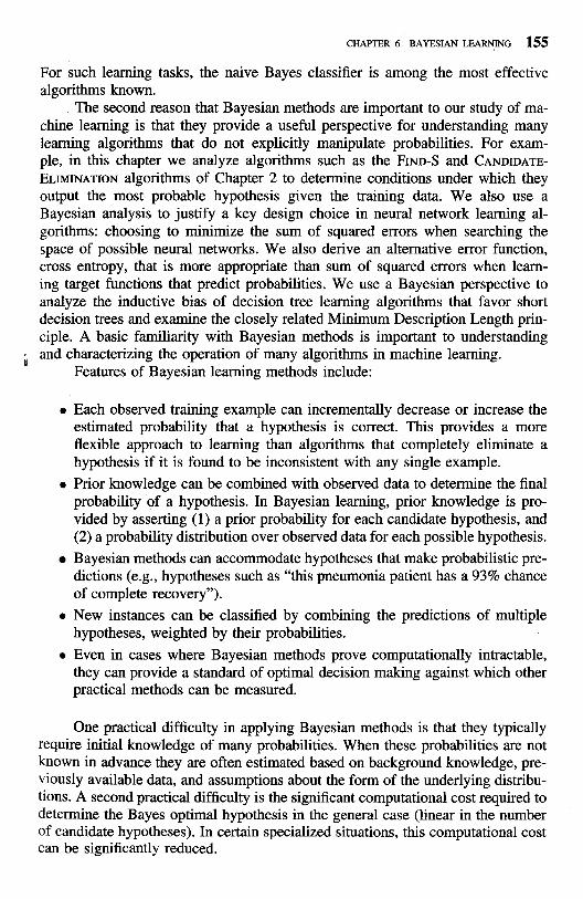
Bayesian reasoning provides a probabilistic approach to inference. It is based on the assumption that the quantities of interest are governed by probability distri- butions and that optimal decisions can be made by reasoning about these proba- bilities together with observed data. It is important to machine learning because it provides a quantitative approach to weighing the evidence supporting alterna- tive hypotheses. Bayesian reasoning provides the basis for learning algorithms that directly manipulate probabilities, as well as a framework for analyzing the operation of other algorithms that do not explicitly manipulate probabilities.
6.1 INTRODUCTION Bayesian learning methods are relevant to our study of machine learning for two different reasons. First, Bayesian learning algorithms that calculate explicit probabilities for hypotheses, such as the naive Bayes classifier, are among the most practical approaches to certain types of learning problems. For example, Michie et al. (1994) provide a detailed study comparing the naive Bayes classifier to other learning algorithms, including decision tree and neural network algorithms. These researchers show that the naive Bayes classifier is competitive with these other learning algorithms in many cases and that in some cases it outperforms these other methods. In this chapter we describe the naive Bayes classifier and provide a detailed example of its use. In particular, we discuss its application to the problem of learning to classify text documents such as electronic news articles.
CHAFER 6 BAYESIAN LEARNING 155
For such learning tasks, the naive Bayes classifier is among the most effective algorithms known.
The second reason that Bayesian methods are important to our study of ma- chine learning is that they provide a useful perspective for understanding many learning algorithms that do not explicitly manipulate probabilities. For exam- ple, in this chapter we analyze algorithms such as the FIND-S and CANDIDATE- ELIMINATION algorithms of Chapter 2 to determine conditions under which they output the most probable hypothesis given the training data. We also use a Bayesian analysis to justify a key design choice in neural network learning al- gorithms: choosing to minimize the sum of squared errors when searching the space of possible neural networks. We also derive an alternative error function, cross entropy, that is more appropriate than sum of squared errors when learn- ing target functions that predict probabilities. We use a Bayesian perspective to analyze the inductive bias of decision tree learning algorithms that favor short decision trees and examine the closely related Minimum Description Length prin- ciple. A basic familiarity with Bayesian methods is important to understanding
U and characterizing the operation of many algorithms in machine learning.
Features of Bayesian learning methods include:
0 Each observed training example can incrementally decrease or increase the estimated probability that a hypothesis is correct. This provides a more flexible approach to learning than algorithms that completely eliminate a hypothesis if it is found to be inconsistent with any single example.
0 Prior knowledge can be combined with observed data to determine the final probability ~f a hypothesis. In Bayesian learning, prior knowledge is pro- vided by asserting (1) a prior probability for each candidate hypothesis, and (2) a probability distribution over observed data for each possible hypothesis. Bayesian methods can accommodate hypotheses that make probabilistic pre- dictions (e.g., hypotheses such as "this pneumonia patient has a 93% chance of complete recovery").
0 New instances can be classified by combining the predictions of multiple hypotheses, weighted by their probabilities.
0 Even in cases where Bayesian methods prove computationally intractable, they can provide a standard of optimal decision making against which other practical methods can be measured.
One practical difficulty in applying Bayesian methods is that they typically require initial knowledge of many probabilities. When these probabilities are not known in advance they are often estimated based on background knowledge, pre- viously available data, and assumptions about the form of the underlying distribu- tions. A second practical difficulty is the significant computational cost required to determine the Bayes optimal hypothesis in the general case (linear in the number of candidate hypotheses). In certain specialized situations, this computational cost can be significantly reduced.
The remainder of this chapter is organized as follows. Section 6.2 intro- duces Bayes theorem and defines maximum likelihood and maximum a posteriori probability hypotheses. The four subsequent sections then apply this probabilistic framework to analyze several issues and learning algorithms discussed in earlier chapters. For example, we show that several previously described algorithms out- put maximum likelihood hypotheses, under certain assumptions. The remaining sections then introduce a number of learning algorithms that explicitly manip- ulate probabilities. These include the Bayes optimal classifier, Gibbs algorithm, and naive Bayes classifier. Finally, we discuss Bayesian belief networks, a rela- tively recent approach to learning based on probabilistic reasoning, and the EM algorithm, a widely used algorithm for learning in the presence of unobserved variables.
6.2 BAYES THEOREM In machine learning we are often interested in determining the best hypothesis from some space H, given the observed training data D. One way to specify what we mean by the best hypothesis is to say that we demand the most probable hypothesis, given the data D plus any initial knowledge about the prior probabil- ities of the various hypotheses in H. Bayes theorem provides a direct method for calculating such probabilities. More precisely, Bayes theorem provides a way to calculate the probability of a hypothesis based on its prior probability, the proba- bilities of observing various data given the hypothesis, and the observed data itself.
To define Bayes theorem precisely, let us first introduce a little notation. We shall write P(h) to denote the initial probability that hypothesis h holds, before we have observed the training data. P(h) is often called the priorprobability of h and may reflect any background knowledge we have about the chance that h is a correct hypothesis. If we have no such prior knowledge, then we might simply assign the same prior probability to each candidate hypothesis. Similarly, we will write P ( D ) to denote the prior probability that training data D will be observed (i.e., the probability of D given no knowledge about which hypothesis holds). Next, we will write P(D1h) to denote the probability of observing data D given some world in which hypothesis h holds. More generally, we write P(xly) to denote the probability of x given y. In machine learning problems we are interested in the probability P (h 1 D ) that h holds given the observed training data D. P (h 1 D ) is called the posteriorprobability of h, because it reflects our confidence that h holds after we have seen the training data D . Notice the posterior probability P(h1D) reflects the influence of the training data D, in contrast to the prior probability P(h) , which is independent of D.
Bayes theorem is the cornerstone of Bayesian learning methods because it provides a way to calculate the posterior probability P(hlD), from the prior probability P(h), together with P ( D ) and P(D(h) .
Bayes theorem:
CHAPTER 6 BAYESIAN LEARNING 157
As one might intuitively expect, P(h ID) increases with P(h) and with P(D1h) according to Bayes theorem. It is also reasonable to see that P(hl D) decreases as P(D) increases, because the more probable it is that D will be observed indepen- dent of h, the less evidence D provides in support of h.
In many learning scenarios, the learner considers some set of candidate hypotheses H and is interested in finding the most probable hypothesis h E H given the observed data D (or at least one of the maximally probable if there are several). Any such maximally probable hypothesis is called a maximum a posteriori (MAP) hypothesis. We can determine the MAP hypotheses by using Bayes theorem to calculate the posterior probability of each candidate hypothesis. More precisely, we will say that MAP is a MAP hypothesis provided
h ~ ~ p = argmax P(hlD) h€H
= argmax P(D 1 h) P (h) h€H
(6.2)
Notice in the final step above we dropped the term P ( D ) because it is a constant independent of h.
In some cases, we will assume that every hypothesis in H is equally probable a priori (P(hi ) = P(h;) for all hi and h; in H). In this case we can further simplify Equation (6.2) and need only consider the term P(D1h) to find the most probable hypothesis. P(Dlh) is often called the likelihood of the data D given h, and any hypothesis that maximizes P(Dlh) is called a maximum likelihood (ML) hypothesis, hML.
hML = argmax P(Dlh) h €H
In order to make clear the connection to machine learning problems, we introduced Bayes theorem above by referring to the data D as training examples of some target function and referring to H as the space of candidate target functions. In fact, Bayes theorem is much more general than suggested by this discussion. It can be applied equally well to any set H of mutually exclusive propositions whose probabilities sum to one (e.g., "the sky is blue," and "the sky is not blue"). In this chapter, we will at times consider cases where H is a hypothesis space containing possible target functions and the data D are training examples. At other times we will consider cases where H is some other set of mutually exclusive propositions, and D is some other kind of data.
6.2.1 An Example To illustrate Bayes rule, consider a medical diagnosis problem in which there are two alternative hypotheses: (1) that the patien; has a- articular form of cancer. and (2) that the patient does not. The avaiiable data is from a particular laboratory
test with two possible outcomes: $ (positive) and 8 (negative). We have prior knowledge that over the entire population of people only .008 have this disease. Furthermore, the lab test is only an imperfect indicator of the disease. The test returns a correct positive result in only 98% of the cases in which the disease is actually present and a correct negative result in only 97% of the cases in which the disease is not present. In other cases, the test returns the opposite result. The above situation can be summarized by the following probabilities:
Suppose we now observe a new patient for whom the lab test returns a positive result. Should we diagnose the patient as having cancer or not? The maximum a posteriori hypothesis can be found using Equation (6.2):
Thus, h ~ ~ p = -cancer. The exact posterior hobabilities can also be determined by normalizing the above quantities so that they sum to 1 (e.g., P(cancer($) = .00;~~298 = .21). This step is warranted because Bayes theorem states that the posterior probabilities are just the above quantities divided by the probability of the data, P(@). Although P($) was not provided directly as part of the problem statement, we can calculate it in this fashion because we know that P(cancerl$) and P(-cancerl$) must sum to 1 (i.e., either the patient has cancer or they do not). Notice that while the posterior probability of cancer is significantly higher than its prior probability, the most probable hypothesis is still that the patient does not have cancer.
As this example illustrates, the result of Bayesian inference depends strongly on the prior probabilities, which must be available in order to apply the method directly. Note also that in this example the hypotheses are not completely accepted or rejected, but rather become more or less probable as more data is observed.
Basic formulas for calculating probabilities are summarized in Table 6.1.
6.3 BAYES THEOREM AND CONCEPT LEARNING What is the relationship between Bayes theorem and the problem of concept learn- ing? Since Bayes theorem provides a principled way to calculate the posterior probability of each hypothesis given the training data, we can use it as the basis for a straightforward learning algorithm that calculates the probability for each possible hypothesis, then outputs the most probable. This section considers such a brute-force Bayesian concept learning algorithm, then compares it to concept learning algorithms we considered in Chapter 2. As we shall see, one interesting result of this comparison is that under certain conditions several algorithms dis- cussed in earlier chapters output the same hypotheses as this brute-force Bayesian
CHAPTER 6 BAYESIAN LEARNING 159 - . Product rule: probability P ( A A B) of a conjunction of two events A and B
Sum rule: probability of a disjunction of two events A and B
Bayes theorem: the posterior probability P(hl D ) of h given D
. Theorem of totalprobability: if events A 1 , . . . , A, are mutually exclusive with xy=l P ( A i ) = 1 , then
TABLE 6.1 Summary of basic probability formulas.
11
t algorithm, despite the fact that they do not explicitly manipulate probabilities and are considerably more efficient.
6.3.1 Brute-Force Bayes Concept Learning Consider the concept learning problem first introduced in Chapter 2. In particular, assume the learner considers some finite hypothesis space H defined over the instance space X, in which the task is to learn some target concept c : X + {0,1}. As usual, we assume that the learner is given some sequence of training examples ( ( x ~ , d l ) . . . (xm, dm)) where xi is some instance from X and where di is the target value of xi (i.e., di = c(xi)). To simplify the discussion in this section, we assume the sequence of instances (xl . . . xm) is held fixed, so that the training data D can be written simply as the sequence of target values D = (dl . . . dm) . It can be shown (see Exercise 6.4) that this simplification does not alter the main conclusions of this section.
We can design a straightforward concept learning algorithm to output the maximum a posteriori hypothesis, based on Bayes theorem, as follows:
BRUTE-FORCE MAP LEARNING algorithm 1. For each hypothesis h in H, calculate the posterior probability
2. Output the hypothesis hMAP with the highest posterior probability
160 MACHINE LEARNING
This algorithm may require significant computation, because it applies Bayes theo- rem to each hypothesis in H to calculate P(hJ D ) . While this may prove impractical for large hypothesis spaces, the algorithm is still of interest because it provides a standard against which we may judge the performance of other concept learning algorithms.
In order specify a Iearning problem for the BRUTE-FORCE MAP LEARNING algorithm we must specify what values are to be used for P(h) and for P(D1h) (as we shall see, P ( D ) will be determined once we choose the other two). We may choose the probability distributions P(h) and P(D1h) in any way we wish, to describe our prior knowledge about the learning task. Here let us choose them to be consistent with the following assumptions:
1. The training data D is noise free (i.e., di = c(xi) ) .
2. The target concept c is contained in the hypothesis space H
3. We have no a priori reason to believe that any hypothesis is more probable than any other.
Given these assumptions, what values should we specify for P(h)? Given no prior knowledge that one hypothesis is more likely than another, it is reasonable to assign the same prior probability to every hypothesis h in H . Furthermore, because we assume the target concept is contained in H we should require that these prior probabilities sum to 1. Together these constraints imply that we should choose
1 P(h) = - for all h in H
IHI
What choice shall we make for P(Dlh)? P(D1h) is the probability of ob- serving the target values D = (dl . . .dm) for the fixed set of instances ( X I . . . x,), given a world in which hypothesis h holds (i.e., given a world in which h is the correct description of the target concept c). Since we assume noise-free training data, the probability of observing classification di given h is just 1 if di = h(xi) and 0 if di # h(xi). Therefore,
1 if di = h(xi) for all di in D P(D1h) = (6.4)
0 otherwise
In other words, the probability of data D given hypothesis h is 1 if D is consistent with h, and 0 otherwise.
Given these choices for P(h) and for P(Dlh) we now have a fully-defined problem for the above BRUTE-FORCE MAP LEARNING algorithm. Let us consider the first step of this algorithm, which uses Bayes theorem to compute the posterior probability P(h1D) of each hypothesis h given the observed training data D .
CHAPTER 6 BAYESIAN LEARNING 161
Recalling Bayes theorem, we have
First consider the case where h is inconsistent with the training data D. Since Equation (6.4) defines P(D)h ) to be 0 when h is inconsistent with D, we have
P ( ~ ( D ) = - ' P(h) - - o if h is inconsistent with D P(D)
The posterior probability of a hypothesis inconsistent with D is zero. Now consider the case where h is consistent with D. Since Equation (6.4)
defines P(Dlh) to be 1 when h is consistent with D, we have
- 1 -- if h is consistent with D IVSH,DI
where V S H , ~ is the subset of hypotheses from H that are consistent with D (i.e., V S H , ~ is the version space of H with respect to D as defined in Chapter 2). It is easy to verify that P(D) = above, because the sum over all hypotheses of P(h ID) must be one and because the number of hypotheses from H consistent with D is by definition IVSH,DI. Alternatively, we can derive P(D) from the theorem of total probability (see Table 6.1) and the fact that the hypotheses are mutually exclusive (i.e., (Vi # j ) (P(hi A hj ) = 0 ) )
To summarize, Bayes theorem implies that the posterior probability P(h ID) under our assumed P(h) and P(D1h) is
if h is consistent with D P(hlD) = (6 .3
0 otherwise
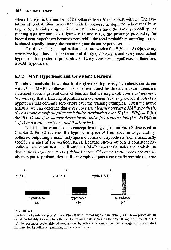
where IVSH,DI is the number of hypotheses from H consistent with D. The evo- lution of probabilities associated with hypotheses is depicted schematically in Figure 6.1. Initially (Figure 6 . 1 ~ ) all hypotheses have the same probability. As training data accumulates (Figures 6.1 b and 6. lc), the posterior probability for inconsistent hypotheses becomes zero while the total probability summing to one is shared equally among the remaining consistent hypotheses.
The above analysis implies that under our choice for P(h) and P(Dlh), every consistent hypothesis has posterior probability (1 / I V SH, I), and every inconsistent hypothesis has posterior probability 0. Every consistent hypothesis is, therefore, a MAP hypothesis.
6.3.2 MAP Hypotheses and Consistent Learners The above analysis shows that in the given setting, every hypothesis consistent with D is a MAP hypothesis. This statement translates directly into an interesting statement about a general class of learners that we might call consistent learners. We will say that a learning algorithm is a consistent learner provided it outputs a hypothesis that commits zero errors over the training examples. Given the above analysis, we can conclude that every consistent learner outputs a MAP hypothesis, i f we assume a uniform prior probability distribution over H (i.e., P(hi) = P(hj) for all i, j ) , and ifwe assume deterministic, noise free training data (i.e., P(D Ih) = 1 i f D and h are consistent, and 0 otherwise).
Consider, for example, the concept learning algorithm FIND-S discussed in Chapter 2. FIND-S searches the hypothesis space H from specific to general hy- potheses, outputting a maximally specific consistent hypothesis (i.e., a maximally specific member of the version space). Because FIND-S outputs a consistent hy- pothesis, we know that it will output a MAP hypothesis under the probability distributions P(h) and P(D1h) defined above. Of course FIND-S does not explic- itly manipulate probabilities at all-it simply outputs a maximally specific member
hypotheses hypotheses ( a ) (4
hypotheses ( c )
FIGURE 6.1 Evolution of posterior probabilities P(hlD) with increasing training data. (a) Uniform priors assign equal probability to each hypothesis. As training data increases first to Dl (b), then to Dl A 0 2 (c), the posterior probability of inconsistent hypotheses becomes zero, while posterior probabilities increase for hypotheses remaining in the version space.
CHAPTER 6 BAYESIAN LEARNING 163
of the version space. However, by identifying distributions for P ( h ) and P ( D ( h ) under which its output hypotheses will be MAP hypotheses, we have a useful way of characterizing the behavior of FIND-S.
Are there other probability distributions for P(h) and P(D1h) under which FIND-S outputs MAP hypotheses? Yes. Because FIND-S outputs a maximally spe- cz$c hypothesis from the version space, its output hypothesis will be a MAP hypothesis relative to any prior probability distribution that favors more specific hypotheses. More precisely, suppose 3-1 is any probability distribution P(h) over H that assigns P(h1) 2 P(hz ) if hl is more specific than h2. Then it can be shown that FIND-S outputs a MAP hypothesis assuming the prior distribution 3-1 and the same distribution P(D1h) discussed above.
To summarize the above discussion, the Bayesian framework allows one way to characterize the behavior of learning algorithms (e.g., FIND-S), even when the learning algorithm does not explicitly manipulate probabilities. By identifying probability distributions P(h) and P(Dlh) under which the algorithm outputs optimal (i.e., MAP) hypotheses, we can characterize the implicit assumptions
, under which this algorithm behaves optimally. ( Using the Bayesian perspective to characterize learning algorithms in this
way is similar in spirit to characterizing the inductive bias of the learner. Recall that in Chapter 2 we defined the inductive bias of a learning algorithm to be the set of assumptions B sufficient to deductively justify the inductive inference performed by the learner. For example, we described the inductive bias of the CANDIDATE-ELIMINATION algorithm as the assumption that the target concept c is included in the hypothesis space H. Furthermore, we showed there that the output of this learning algorithm follows deductively from its inputs plus this implicit inductive bias assumption. The above Bayesian interpretation provides an alter- native way to characterize the assumptions implicit in learning algorithms. Here, instead of modeling the inductive inference method by an equivalent deductive system, we model it by an equivalent probabilistic reasoning system based on Bayes theorem. And here the implicit assumptions that we attribute to the learner are assumptions of the form "the prior probabilities over H are given by the distribution P(h) , and the strength of data in rejecting or accepting a hypothesis is given by P(Dlh)." The definitions of P(h) and P ( D ( h ) given in this section characterize the implicit assumptions of the CANDIDATE-ELIMINATION and FIND-S algorithms. A probabilistic reasoning system based on Bayes theorem will exhibit input-output behavior equivalent to these algorithms, provided it is given these assumed probability distributions.
The discussion throughout this section corresponds to a special case of Bayesian reasoning, because we considered the case where P(D1h) takes on val- ues of only 0 and 1, reflecting the deterministic predictions of hypotheses and the assumption of noise-free training data. As we shall see in the next section, we can also model learning from noisy training data, by allowing P(D1h) to take on values other than 0 and 1, and by introducing into P(D1h) additional assumptions about the probability distributions that govern the noise.
6.4 MAXIMUM LIKELIHOOD AND LEAST-SQUARED ERROR HYPOTHESES As illustrated in the above section, Bayesian analysis can sometimes be used to show that a particular learning algorithm outputs MAP hypotheses even though it may not explicitly use Bayes rule or calculate probabilities in any form.
In this section we consider the problem of learning a continuous-valued target function-a problem faced by many learning approaches such as neural network learning, linear regression, and polynomial curve fitting. A straightfor- ward Bayesian analysis will show that under certain assumptions any learning algorithm that minimizes the squared error between the output hypothesis pre- dictions and the training data will output a maximum likelihood hypothesis. The significance of this result is that it provides a Bayesian justification (under cer- tain assumptions) for many neural network and other curve fitting methods that attempt to minimize the sum of squared errors over the training data.
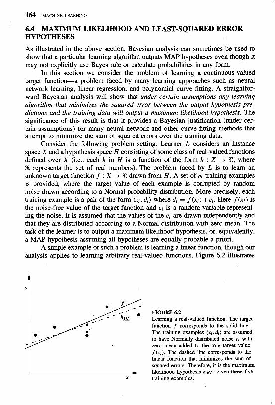
Consider the following problem setting. Learner L considers an instance space X and a hypothesis space H consisting of some class of real-valued functions defined over X (i.e., each h in H is a function of the form h : X -+ 8, where 8 represents the set of real numbers). The problem faced by L is to learn an unknown target function f : X -+ 8 drawn from H. A set of m training examples is provided, where the target value of each example is corrupted by random noise drawn according to a Normal probability distribution. More precisely, each training example is a pair of the form (xi, d i ) where di = f (xi) + ei. Here f (xi) is the noise-free value of the target function and ei is a random variable represent- ing the noise. It is assumed that the values of the ei are drawn independently and that they are distributed according to a Normal distribution with zero mean. The task of the learner is to output a maximum likelihood hypothesis, or, equivalently, a MAP hypothesis assuming all hypotheses are equally probable a priori.
A simple example of such a problem is learning a linear function, though our analysis applies to learning arbitrary real-valued functions. Figure 6.2 illustrates
FIGURE 6.2 Learning a real-valued function. The target function f corresponds to the solid line. The training examples (xi, di ) are assumed to have Normally distributed noise ei with zero mean added to the true target value f (xi). The dashed line corresponds to the linear function that minimizes the sum of squared errors. Therefore, it is the maximum
I likelihood hypothesis ~ M L , given these five x training examples.
CHAPTER 6 BAYESIAN LEARNING 165
a linear target function f depicted by the solid line, and a set of noisy training examples of this target function. The dashed line corresponds to the hypothesis hML with least-squared training error, hence the maximum likelihood hypothesis. Notice that the maximum likelihood hypothesis is not necessarily identical to the correct hypothesis, f , because it is inferred from only a limited sample of noisy training data.
Before showing why a hypothesis that minimizes the sum of squared errors in this setting is also a maximum likelihood hypothesis, let us quickly review two basic concepts from probability theory: probability densities and Normal distribu- tions. First, in order to discuss probabilities over continuous variables such as e, we must introduce probability densities. The reason, roughly, is that we wish for the total probability over all possible values of the random variable to sum to one. In the case of continuous variables we cannot achieve this by assigning a finite probability to each of the infinite set of possible values for the random variable. Instead, we speak of a probability density for continuous variables such as e and require that the integral of this probability density over all possible values be one. In general we will use lower case p to refer to the probability density function, to distinguish it from a finite probability P (which we will sometimes refer to as a probability mass). The probability density p(x0) is the limit as E goes to zero, of times the probability that x will take on a value in the interval [xo, xo + 6 ) .
Probability density function:
Second, we stated that the random noise variable e is generated by a Normal probability distribution. A Normal distribution is a smooth, bell-shaped distribu- tion that can be completely characterized by its mean p and its standard deviation a. See Table 5.4 for a precise definition.
Given this background we now return to the main issue: showing that the least-squared error hypothesis is, in fact, the maximum likelihood hypothesis within our problem setting. We will show this by deriving the maximum like- lihood hypothesis starting with our earlier definition Equation (6.3), but using lower case p to refer to the probability density
As before, we assume a fixed set of training instances (xl . . . xm) and there- fore consider the data D to be the corresponding sequence of target values D = (d l . . . d m ) . Here di = f (x i ) + ei. Assuming the training examples are mu- tually independent given h, we can write P ( D J h ) as the product of the various ~ ( d i lh)
Given that the noise ei obeys a Normal distribution with zero mean and unknown variance a 2 , each di must also obey a Normal distribution with variance a2 cen- tered around the true target value f (x i ) rather than zero. Therefore p(di lh) can be written as a Normal distribution with variance a2 and mean p = f (x i ) . Let us write the formula for this Normal distribution to describe p(di Ih), beginning with the general formula for a Normal distribution from Table 5.4 and substituting the appropriate p and a 2 . Because we are writing the expression for the probability of di given that h is the correct description of the target function f , we will also substitute p = f (x i ) = h(xi) , yielding
We now apply a transformation that is common in maximum likelihood calcula- tions: Rather than maximizing the above complicated expression we shall choose to maximize its (less complicated) logarithm. This is justified because lnp is a monotonic function of p. Therefore maximizing In p also maximizes p.
... 1 1 hML = argmax x l n - - -(di - h ( ~ i ) ) ~ h€H i=l dG7 202
The first term in this expression is a constant independent of h, and can therefore be discarded, yielding
1 hMr = argmax C -s(di - h(xi)12
h€H i=l
Maximizing this negative quantity is equivalent to minimizing the corresponding positive quantity.
Finally, we can again discard constants that are independent of h.
Thus, Equation (6.6) shows that the maximum likelihood hypothesis ~ M L is the one that minimizes the sum of the squared errors between the observed training values di and the hypothesis predictions h(x i ) . This holds under the assumption that the observed training values di are generated by adding random noise to
CHAPTER 6 BAYESIAN LEARNING 167
the true target value, where this random noise is drawn independently for each example from a Normal distribution with zero mean. As the above derivation makes clear, the squared error term (di - h ( ~ ~ ) ) ~ follows directly from the exponent in the definition of the Normal distribution. Similar derivations can be performed starting with other assumed noise distributions, producing different results.
Notice the structure of the above derivation involves selecting the hypothesis that maximizes the logarithm of the likelihood (In p(D1h)) in order to determine the most probable hypothesis. As noted earlier, this yields the same result as max- imizing the likelihood p(D1h). This approach of working with the log likelihood is common to many Bayesian analyses, because it is often more mathematically tractable than working directly with the likelihood. Of course, as noted earlier, the maximum likelihood hypothesis might not be the MAP hypothesis, but if one assumes uniform prior probabilities over the hypotheses then it is.
Why is it reasonable to choose the Normal distribution to characterize noise? One reason, it must be admitted, is that it allows for a mathematically straightfor- ward analysis. A second reason is that the smooth, bell-shaped distribution is a good approximation to many types of noise in physical systems. In fact, the Cen- i tral Limit Theorem discussed in Chapter 5 shows that the sum of a sufficiently large number of independent, identically distributed random variables itself obeys a Normal distribution, regardless of the distributions of the individual variables. This implies that noise generated by the sum of very many independent, but identically distributed factors will itself be Normally distributed. Of course, in reality, different components that contribute to noise might not follow identical distributions, in which case this theorem will not necessarily justify our choice.
Minimizing the sum of squared errors is a common approach in many neural network, curve fitting, and other approaches to approximating real-valued func- tions. Chapter 4 describes gradient descent methods that seek the least-squared error hypothesis in neural network learning.
Before leaving our discussion of the relationship between the maximum likelihood hypothesis and the least-squared error hypothesis, it is important to note some limitations of this problem setting. The above analysis considers noise only in the target value of the training example and does not consider noise in the attributes describing the instances themselves. For example, if the problem is to learn to predict the weight of someone based on that person's age and height, then the above analysis assumes noise in measurements of weight, but perfect measurements of age and height. The analysis becomes significantly more complex as these simplifying assumptions are removed.
6.5 MAXIMUM LIKELIHOOD HYPOTHESES FOR PREDICTING PROBABILITIES In the problem setting of the previous section we determined that the maximum likelihood hypothesis is the one that minimizes the sum of squared errors over the training examples. In this section we derive an analogous criterion for a second setting that is common in neural network learning: learning to predict probabilities.
Consider the setting in which we wish to learn a nondeterministic (prob- abilistic) function f : X -+ {0, 11, which has two discrete output values. For example, the instance space X might represent medical patients in terms of their symptoms, and the target function f (x) might be 1 if the patient survives the disease and 0 if not. Alternatively, X might represent loan applicants in terms of their past credit history, and f (x) might be 1 if the applicant successfully repays their next loan and 0 if not. In both of these cases we might well expect f to be probabilistic. For example, among a collection of patients exhibiting the same set of observable symptoms, we might find that 92% survive, and 8% do not. This unpredictability could arise from our inability to observe all the important distin- guishing features of the patients, or from some genuinely probabilistic mechanism in the evolution of the disease. Whatever the source of the problem, the effect is that we have a target function f (x) whose output is a probabilistic function of the input.
Given this problem setting, we might wish to learn a neural network (or other real-valued function approximator) whose output is the probability that f (x) = 1. In other words, we seek to learn the target function, f ' : X + [O, 11, such that f '(x) = P ( f (x) = 1). In the above medical patient example, if x is one of those indistinguishable patients of which 92% survive, then f'(x) = 0.92 whereas the probabilistic function f (x) will be equal to 1 in 92% of cases and equal to 0 in the remaining 8%.
How can we learn f' using, say, a neural network? One obvious, brute- force way would be to first collect the observed frequencies of 1's and 0's for each possible value of x and to then train the neural network to output the target frequency for each x. As we shall see below, we can instead train a neural network directly from the observed training examples of f, yet still derive a maximum likelihood hypothesis for f '.
What criterion should we optimize in order to find a maximum likelihood hypothesis for f' in this setting? To answer this question we must first obtain an expression for P(D1h). Let us assume the training data D is of the form D = {(xl, dl) . . . (x,, dm)}, where di is the observed 0 or 1 value for f (xi).
Recall that in the maximum likelihood, least-squared error analysis of the previous section, we made the simplifying assumption that the instances (xl . . . x,) were fixed. This enabled us to characterize the data by considering only the target values di. Although we could make a similar simplifying assumption in this case, let us avoid it here in order to demonstrate that it has no impact on the final outcome. Thus treating both xi and di as random variables, and assuming that each training example is drawn independently, we can write P(D1h) as
m
P(Dlh) = n ,(xi, 41,) (6.7) i=l
It is reasonable to assume, furthermore, that the probability of encountering any particular instance xi is independent of the hypothesis h. For example, the probability that our training set contains a particular patient xi is independent of our hypothesis about survival rates (though of course the survival d, of the patient
CHAPTER 6 BAYESIAN LEARNING 169
does depend strongly on h). When x is independent of h we can rewrite the above expression (applying the product rule from Table 6.1) as
Now what is the probability P(dilh, xi) of observing di = 1 for a single instance xi, given a world in which hypothesis h holds? Recall that h is our hypothesis regarding the target function, which computes this very probability. Therefore, P(di = 1 1 h, xi) = h(xi), and in general
In order to substitute this into the Equation (6.8) for P(Dlh), let us first " re-express it in a more mathematically manipulable form, as I'
It is easy to verify that the expressions in Equations (6.9) and (6.10) are equivalent. Notice that when di = 1 , the second term from Equation (6.10), ( 1 - h(xi))'-", becomes equal to 1. Hence P(di = l lh,xi) = h(xi), which is equivalent to the first case in Equation (6.9). A similar analysis shows that the two equations are also equivalent when di = 0.
We can use Equation (6.10) to substitute for P(di lh, xi) in Equation (6.8) to obtain
Now we write an expression for the maximum likelihood hypothesis
The last term is a constant independent of h, so it can be dropped
The expression on the right side of Equation (6.12) can be seen as a gen- eralization of the Binomial distribution described in Table 5.3. The expression in Equation (6.12) describes the probability that flipping each of m distinct coins will produce the outcome (dl . . .dm), assuming that each coin xi has probability h(xi) of producing a heads. Note the Binomial distribution described in Table 5.3 is
similar, but makes the additional assumption that the coins have identical proba- bilities of turning up heads (i.e., that h(xi) = h(xj), Vi, j). In both cases we assume the outcomes of the coin flips are mutually independent-an assumption that fits our current setting.
As in earlier cases, we will find it easier to work with the log of the likeli- hood, yielding
Equation (6.13) describes the quantity that must be maximized in order to obtain the maximum likelihood hypothesis in our current problem setting. This result is analogous to our earlier result showing that minimizing the sum of squared errors produces the maximum likelihood hypothesis in the earlier problem setting. Note the similarity between Equation (6.13) and the general form of the entropy function, -xi pi log pi, discussed in Chapter 3. Because of this similarity, the negation of the above quantity is sometimes called the cross entropy.
6.5.1 Gradient Search to Maximize Likelihood in a Neural Net Above we showed that maximizing the quantity in Equation (6.13) yields the maximum likelihood hypothesis. Let us use G(h, D) to denote this quantity. In this section we derive a weight-training rule for neural network learning that seeks to maximize G(h, D) using gradient ascent.
As discussed in Chapter 4, the gradient of G(h, D) is given by the vector of partial derivatives of G(h, D) with respect to the various network weights that define the hypothesis h represented by the learned network (see Chapter 4 for a general discussion of gradient-descent search and for details of the terminology that we reuse here). In this case, the partial derivative of G(h, D) with respect to weight wjk from input k to unit j is
To keep our analysis simple, suppose our neural network is constructed from a single layer of sigmoid units. In this case we have
where xijk is the kth input to unit j for the ith training example, and d ( x ) is the derivative of the sigmoid squashing function (again, see Chapter 4). Finally,
CIUPlER 6 BAYESIAN LEARNING 171
substituting this expression into Equation (6.14), we obtain a simple expression for the derivatives that constitute the gradient
Because we seek to maximize rather than minimize P(D(h), we perform gradient ascent rather than gradient descent search. On each iteration of the search the weight vector is adjusted in the direction of the gradient, using the weight- update rule
where m
Awjk = 7 C ( d i - hbi)) xijk (6.15) i=l
and where 7 is a small positive constant that determines the step size of the i gradient ascent search. It is interesting to compare this weight-update rule to the weight-update
rule used by the BACKPROPAGATION algorithm to minimize the sum of squared errors between predicted and observed network outputs. The BACKPROPAGATION update rule for output unit weights (see Chapter 4), re-expressed using our current notation, is
where
Notice this is similar to the rule given in Equation (6.15) except for the extra term h ( x , ) ( l - h(xi)), which is the derivative of the sigmoid function.
To summarize, these two weight update rules converge toward maximum likelihood hypotheses in two different settings. The rule that minimizes sum of squared error seeks the maximum likelihood hypothesis under the assumption that the training data can be modeled by Normally distributed noise added to the target function value. The rule that minimizes cross entropy seeks the maximum likelihood hypothesis under the assumption that the observed boolean value is a probabilistic function of the input instance.
6.6 MINIMUM DESCRIPTION LENGTH PRINCIPLE Recall from Chapter 3 the discussion of Occam's razor, a popular inductive bias that can be summarized as "choose the shortest explanation for the observed data." In that chapter we discussed several arguments in the long-standing debate regarding Occam's razor. Here we consider a Bayesian perspective on this issue
and a closely related principle called the Minimum Description Length (MDL) principle.
The Minimum Description Length principle is motivated by interpreting the definition of h M ~ p in the light of basic concepts from information theory. Consider again the now familiar definition of MAP.
hMAP = argmax P(Dlh)P(h) h€H
which can be equivalently expressed in terms of maximizing the log,
MAP = argmax log2 P ( D lh) + log, P ( h ) h€H
or alternatively, minimizing the negative of this quantity
hMAp = argmin - log, P ( D 1 h ) - log, P(h) h€H
Somewhat surprisingly, Equation (6.16) can be interpreted as a statement that short hypotheses are preferred, assuming a particular representation scheme for encoding hypotheses and data. To explain this, let us introduce a basic result from information theory: Consider the problem of designing a code to transmit messages drawn at random, where the probability of encountering message i is pi. We are interested here in the most compact code; that is, we are interested in the code that minimizes the expected number of bits we must transmit in order to encode a message drawn at random. Clearly, to minimize the expected code length we should assign shorter codes to messages that are more probable. Shannon and Weaver (1949) showed that the optimal code (i.e., the code that minimizes the expected message length) assigns - log, pi bitst to encode message i . We will refer to the number of bits required to encode message i using code C as the description length of message i with respect to C , which we denote by Lc( i ) .
Let us interpret Equation (6.16) in light of the above result from coding theory.
0 - log, P ( h ) is the description length of h under the optimal encoding for the hypothesis space H. In other words, this is the size of the description of hypothesis h using this optimal representation. In our notation, LC, (h) = - log, P(h) , where CH is the optimal code for hypothesis space H.
0 -log2 P(D1h) is the description length of the training data D given hypothesis h, under its optimal encoding. In our notation, Lc,,,(Dlh) = - log, P(Dlh) , where C D , ~ is the optimal code for describing data D assum- ing that both the sender and receiver know the hypothesis h .
t ~ o t i c e the expected length for transmitting one message is therefore xi -pi logz pi, the formula for the entropy (see Chapter 3) of the set of possible messages.
CHAPTER 6 BAYESIAN LEARNING 173
0 Therefore we can rewrite Equation (6.16) to show that hMAP is the hypothesis h that minimizes the sum given by the description length of the hypothesis plus the description length of the data given the hypothesis.
where CH and CDlh are the optimal encodings for H and for D given h, respectively.
The Minimum Description Length (MDL) principle recommends choosing the hypothesis that minimizes the sum of these two description lengths. Of course to apply this principle in practice we must choose specific encodings or represen- tations appropriate for the given learning task. Assuming we use the codes C1 and CZ to represent the hypothesis and the data given the hypothesis, we can state the MDL principle as
1'
I Minimum Description Length principle: Choose hMDL where
The above analysis shows that if we choose C1 to be the optimal encoding of hypotheses CH, and if we choose C2 to be the optimal encoding CDlh, then ~ M D L = A MAP.
Intuitively, we can think of the MDL principle as recommending the shortest method for re-encoding the training data, where we count both the size of the hypothesis and any additional cost of encoding the data given this hypothesis.
Let us consider an example. Suppose we wish to apply the MDL prin- ciple to the problem of learning decision trees from some training data. What should we choose for the representations C1 and C2 of hypotheses and data? For C1 we might naturally choose some obvious encoding of decision trees, in which the description length grows with the number of nodes in the tree and with the number of edges. How shall we choose the encoding C2 of the data given a particular decision tree hypothesis? To keep things simple, suppose that the sequence of instances (xl . . .x,) is already known to both the transmitter and receiver, so that we need only transmit the classifications (f (XI) . . . f (x,)). (Note the cost of transmitting the instances themselves is independent of the cor- rect hypothesis, so it does not affect the selection of ~ M D L in any case.) Now if the training classifications (f (xl) . . . f (xm)) are identical to the predictions of the hypothesis, then there is no need to transmit any information about these exam- ples (the receiver can compute these values once it has received the hypothesis). The description length of the classifications given the hypothesis in this case is, therefore, zero. In the case where some examples are misclassified by h, then for each misclassification we need to transmit a message that identifies which example is misclassified (which can be done using at most logzm bits) as well
as its correct classification (which can be done using at most log2 k bits, where k is the number of possible classifications). The hypothesis hMDL under the en- coding~ C1 and C2 is just the one that minimizes the sum of these description lengths.
Thus the MDL principle provides a way of trading off hypothesis complexity for the number of errors committed by the hypothesis. It might select a shorter hypothesis that makes a few errors over a longer hypothesis that perfectly classifies the training data. Viewed in this light, it provides one method for dealing with the issue of overjitting the data.
Quinlan and Rivest (1989) describe experiments applying the MDL principle to choose the best size for a decision tree. They report that the MDL-based method produced learned trees whose accuracy was comparable to that of the standard tree- pruning methods discussed in Chapter 3. Mehta et al. (1995) describe an alternative MDL-based approach to decision tree pruning, and describe experiments in which an MDL-based approach produced results comparable to standard tree-pruning methods.
What shall we conclude from this analysis of the Minimum Description Length principle? Does this prove once and for all that short hypotheses are best? No. What we have shown is only that ifa representation of hypotheses is chosen so that the size of hypothesis h is - log2 P(h), and ifa representation for exceptions is chosen so that the encoding length of D given h is equal to -log2 P(Dlh), then the MDL principle produces MAP hypotheses. However, to show that we have such a representation we must know all the prior probabilities P(h), as well as the P(D1h). There is no reason to believe that the MDL hypothesis relative to arbitrary encodings C1 and C2 should be preferred. As a practical matter it might sometimes be easier for a human designer to specify a representation that captures knowledge about the relative probabilities of hypotheses than it is to fully specify the probability of each hypothesis. Descriptions in the literature on the application of MDL to practical learning problems often include arguments providing some form of justification for the encodings chosen for C1 and C2.
6.7 BAYES OPTIMAL CLASSIFIER So far we have considered the question "what is the most probable hypothesis given the training data?' In fact, the question that is often of most significance is the closely related question "what is the most probable classiJication of the new instance given the training data?'Although it may seem that this second question can be answered by simply applying the MAP hypothesis to the new instance, in fact it is possible to do better.
To develop some intuitions consider a hypothesis space containing three hypotheses, hl, h2, and h3. Suppose that the posterior probabilities of these hy- potheses given the training data are .4, .3, and .3 respectively. Thus, hl is the MAP hypothesis. Suppose a new instance x is encountered, which is classified positive by h l , but negative by h2 and h3. Taking all hypotheses into account, the probability that x is positive is .4 (the probability associated with hi ) , and
CHAFER 6 BAYESIAN LEARNING 175
the probability that it is negative is therefore .6. The most probable classification (negative) in this case is different from the classification generated by the MAP hypothesis.
In general, the most probable classification of the new instance is obtained by combining the predictions of all hypotheses, weighted by their posterior prob- abilities. If the possible classification of the new example can take on any value v j from some set V, then the probability P(vjlD) that the correct classification for the new instance is v;, is just
The optimal classification of the new instance is the value v,, for which P (v; 1 D) is maximum.
Bayes optimal classification:
To illustrate in terms of the above example, the set of possible classifications of the new instance is V = (@, 81, and
therefore
and
Any system that classifies new instances according to Equation (6.18) is called a Bayes optimal classzjier, or Bayes optimal learner. No other classification method using the same hypothesis space and same prior knowledge can outperform this method on average. This method maximizes the probability that the new instance is classified correctly, given the available data, hypothesis space, and prior probabilities over the hypotheses.
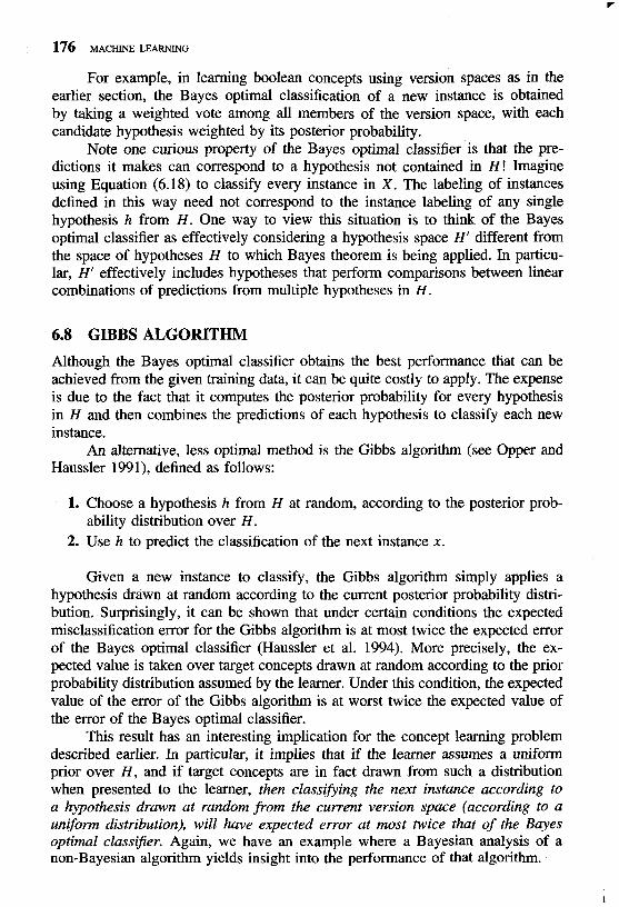
For example, in learning boolean concepts using version spaces as in the earlier section, the Bayes optimal classification of a new instance is obtained by taking a weighted vote among all members of the version space, with each candidate hypothesis weighted by its posterior probability.
Note one curious property of the Bayes optimal classifier is that the pre- dictions it makes can correspond to a hypothesis not contained in H! Imagine using Equation (6.18) to classify every instance in X. The labeling of instances defined in this way need not correspond to the instance labeling of any single hypothesis h from H. One way to view this situation is to think of the Bayes optimal classifier as effectively considering a hypothesis space H' different from the space of hypotheses H to which Bayes theorem is being applied. In particu- lar, H' effectively includes hypotheses that perform comparisons between linear combinations of predictions from multiple hypotheses in H.
6.8 GIBBS ALGORITHM Although the Bayes optimal classifier obtains the best performance that can be achieved from the given training data, it can be quite costly to apply. The expense is due to the fact that it computes the posterior probability for every hypothesis in H and then combines the predictions of each hypothesis to classify each new instance.
An alternative, less optimal method is the Gibbs algorithm (see Opper and Haussler 1991), defined as follows:
1. Choose a hypothesis h from H at random, according to the posterior prob- ability distribution over H.
2. Use h to predict the classification of the next instance x.
Given a new instance to classify, the Gibbs algorithm simply applies a hypothesis drawn at random according to the current posterior probability distri- bution. Surprisingly, it can be shown that under certain conditions the expected misclassification error for the Gibbs algorithm is at most twice the expected error of the Bayes optimal classifier (Haussler et al. 1994). More precisely, the ex- pected value is taken over target concepts drawn at random according to the prior probability distribution assumed by the learner. Under this condition, the expected value of the error of the Gibbs algorithm is at worst twice the expected value of the error of the Bayes optimal classifier.
This result has an interesting implication for the concept learning problem described earlier. In particular, it implies that if the learner assumes a uniform prior over H, and if target concepts are in fact drawn from such a distribution when presented to the learner, then classifying the next instance according to a hypothesis drawn at random from the current version space (according to a uniform distribution), will have expected error at most twice that of the Bayes optimal classijier. Again, we have an example where a Bayesian analysis of a non-Bayesian algorithm yields insight into the performance of that algorithm.
CHAPTJZR 6 BAYESIAN LEARNING 177
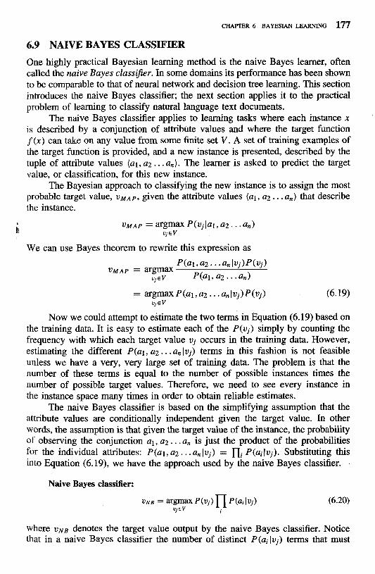
6.9 NAIVE BAYES CLASSIFIER One highly practical Bayesian learning method is the naive Bayes learner, often called the naive Bayes classijier. In some domains its performance has been shown to be comparable to that of neural network and decision tree learning. This section introduces the naive Bayes classifier; the next section applies it to the practical problem of learning to classify natural language text documents.
The naive Bayes classifier applies to learning tasks where each instance x is described by a conjunction of attribute values and where the target function f ( x ) can take on any value from some finite set V. A set of training examples of the target function is provided, and a new instance is presented, described by the tuple of attribute values (a l , a2 . . .a,) . The learner is asked to predict the target value, or classification, for this new instance.
The Bayesian approach to classifying the new instance is to assign the most probable target value, VMAP, given the attribute values ( a l , a2 . . . a,) that describe the instance.
VMAP = argmax P(vj lal , a 2 . . . a,) v j€v
We can use Bayes theorem to rewrite this expression as
Now we could attempt to estimate the two terms in Equation (6.19) based on the training data. It is easy to estimate each of the P(v j ) simply by counting the frequency with which each target value vj occurs in the training data. However, estimating the different P(al , a 2 . . . a,lvj) terms in this fashion is not feasible unless we have a very, very large set of training data. The problem is that the number of these terms is equal to the number of possible instances times the number of possible target values. Therefore, we need to see every instance in the instance space many times in order to obtain reliable estimates.
The naive Bayes classifier is based on the simplifying assumption that the attribute values are conditionally independent given the target value. In other words, the assumption is that given the target value of the instance, the probability of observing the conjunction al , a2 . . .a, is just the product of the probabilities for the individual attributes: P(a1, a2 . . . a, 1 v j ) = ni P(ai lvj) . Substituting this into Equation (6.19), we have the approach used by the naive Bayes classifier.
Naive Bayes classifier:
VNB = argmax P (vj) n P (ai 1vj) (6.20) ujcv
where V N B denotes the target value output by the naive Bayes classifier. Notice that in a naive Bayes classifier the number of distinct P(ailvj) terms that must
be estimated from the training data is just the number of distinct attribute values times the number of distinct target values-a much smaller number than if we were to estimate the P(a1, a2 . . . an lvj) terms as first contemplated.
To summarize, the naive Bayes learning method involves a learning step in which the various P(vj) and P(ai Jvj) terms are estimated, based on their frequen- cies over the training data. The set of these estimates corresponds to the learned hypothesis. This hypothesis is then used to classify each new instance by applying the rule in Equation (6.20). Whenever the naive Bayes assumption of conditional independence is satisfied, this naive Bayes classification VNB is identical to the MAP classification.
One interesting difference between the naive Bayes learning method and other learning methods we have considered is that there is no explicit search through the space of possible hypotheses (in this case, the space of possible hypotheses is the space of possible values that can be assigned to the various P(vj) and P(ailvj) terms). Instead, the hypothesis is formed without searching, simply by counting the frequency of various data combinations within the training examples.
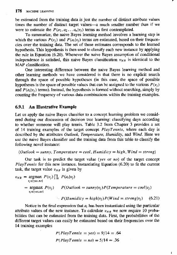
6.9.1 An Illustrative Example Let us apply the naive Bayes classifier to a concept learning problem we consid- ered during our discussion of decision tree learning: classifying days according to whether someone will play tennis. Table 3.2 from Chapter 3 provides a set of 14 training examples of the target concept PlayTennis, where each day is described by the attributes Outlook, Temperature, Humidity, and Wind. Here we use the naive Bayes classifier and the training data from this table to classify the following novel instance:
(Outlook = sunny, Temperature = cool, Humidity = high, Wind = strong) Our task is to predict the target value (yes or no) of the target concept
PlayTennis for this new instance. Instantiating Equation (6.20) to fit the current task, the target value VNB is given by
= argrnax P(vj) P(0utlook = sunny)v,)P(Temperature = coolIvj) vj~(yes,no]
Notice in the final expression that ai has been instantiated using the particular attribute values of the new instance. To calculate VNB we now require 10 proba- bilities that can be estimated from the training data. First, the probabilities of the different target values can easily be estimated based on their frequencies over the 14 training examples
P(P1ayTennis = yes) = 9/14 = .64 P(P1ayTennis = no) = 5/14 = .36
CHAETER 6 BAYESIAN LEARNING 179
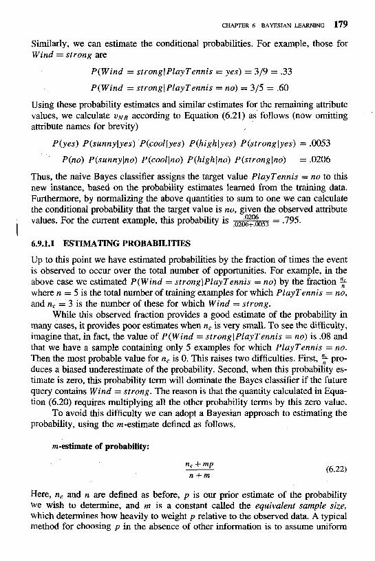
Similarly, we can estimate the conditional probabilities. For example, those for Wind = strong are
P(Wind = stronglPlayTennis = yes) = 319 = .33 P(Wind = strongl PlayTennis = no) = 315 = .60
Using these probability estimates and similar estimates for the remaining attribute values, we calculate V N B according to Equation (6.21) as follows (now omitting attribute names for brevity)
Thus, the naive Bayes classifier assigns the target value PlayTennis = no to this new instance, based on the probability estimates learned from the training data. Furthermore, by normalizing the above quantities to sum to one we can calculate the conditional probability that the target value is no, given the observed attribute values. For the current example, this probability is ,02$ym,, = -795.
6.9.1.1 ESTIMATING PROBABILITIES
Up to this point we have estimated probabilities by the fraction of times the event is observed to occur over the total number of opportunities. For example, in the above case we estimated P(Wind = strong] Play Tennis = no) by the fraction % where n = 5 is the total number of training examples for which PlayTennis = no, and n, = 3 is the number of these for which Wind = strong.
While this observed fraction provides a good estimate of the probability in many cases, it provides poor estimates when n, is very small. To see the difficulty, imagine that, in fact, the value of P(Wind = strongl PlayTennis = no) is .08 and that we have a sample containing only 5 examples for which PlayTennis = no. Then the most probable value for n, is 0 . This raises two difficulties. First, $ pro- duces a biased underestimate of the probability. Second, when this probability es- timate is zero, this probability term will dominate the Bayes classifier if the future query contains Wind = strong. The reason is that the quantity calculated in Equa- tion (6.20) requires multiplying all the other probability terms by this zero value.
To avoid this difficulty we can adopt a Bayesian approach to estimating the probability, using the m-estimate defined as follows.
m-estimate of probability:
Here, n, and n are defined as before, p is our prior estimate of the probability we wish to determine, and m is a constant called the equivalent sample size, which determines how heavily to weight p relative to the observed data. A typical method for choosing p in the absence of other information is to assume uniform
priors; that is, if an attribute has k possible values we set p = i. For example, in estimating P(Wind = stronglPlayTennis = no) we note the attribute Wind has two possible values, so uniform priors would correspond to choosing p = .5. Note that if m is zero, the m-estimate is equivalent to the simple fraction 2. If both n and m are nonzero, then the observed fraction 2 and prior p will be combined according to the weight m. The reason m is called the equivalent sample size is that Equation (6.22) can be interpreted as augmenting the n actual observations by an additional m virtual samples distributed according to p.
6.10 AN EXAMPLE: LEARNING TO CLASSIFY TEXT To illustrate the practical importance of Bayesian learning methods, consider learn- ing problems in which the instances are text documents. For example, we might wish to learn the target concept "electronic news articles that I find interesting," or "pages on the World Wide Web that discuss machine learning topics." In both cases, if a computer could learn the target concept accurately, it could automat- ically filter the large volume of online text documents to present only the most relevant documents to the user.
We present here a general algorithm for learning to classify text, based on the naive Bayes classifier. Interestingly, probabilistic approaches such as the one described here are among the most effective algorithms currently known for learning to classify text documents. Examples of such systems are described by Lewis (1991), Lang (1995), and Joachims (1996).
The naive Bayes algorithm that we shall present applies in the following general setting. Consider an instance space X consisting of all possible text docu- ments (i.e., all possible strings of words and punctuation of all possible lengths). We are given training examples of some unknown target function f ( x ) , which can take on any value from some finite set V. The task is to learn from these training examples to predict the target value for subsequent text documents. For illustration, we will consider the target function classifying documents as interest- ing or uninteresting to a particular person, using the target values like and dislike to indicate these two classes.
The two main design issues involved in applying the naive Bayes classifier to such rext classification problems are first to decide how to represent an arbitrary text document in terms of attribute values, and second to decide how to estimate the probabilities required by the naive Bayes classifier.
Our approach to representing arbitrary text documents is disturbingly simple: Given a text document, such as this paragraph, we define an attribute for each word position in the document and define the value of that attribute to be the English word found in that position. Thus, the current paragraph would be described by 11 1 attribute values, corresponding to the 11 1 word positions. The value of the first attribute is the word "our," the value of the second attribute is the word "approach," and so on. Notice that long text documents will require a larger number of attributes than short documents. As we shall see, this will not cause us any trouble.
CHAPTER 6 BAYESIAN LEARNING 181
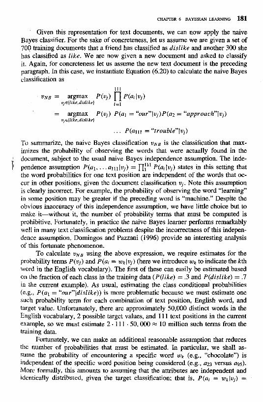
Given this representation for text documents, we can now apply the naive Bayes classifier. For the sake of concreteness, let us assume we are given a set of 700 training documents that a friend has classified as dislike and another 300 she has classified as like. We are now given a new document and asked to classify it. Again, for concreteness let us assume the new text document is the preceding paragraph. In this case, we instantiate Equation (6.20) to calculate the naive Bayes classification as
-a-
Vns = argmax P(Vj) n ~ ( a i lvj) vj~{like,dislike} i=l
- - argmax P(vj) P(a1 = "our"lvj)P(a2 = "approach"lvj) v, ~{like,dislike}
To summarize, the naive Bayes classification VNB is the classification that max- imizes the probability of observing the words that were actually found in the
I document, subject to the usual naive Bayes independence assumption. The inde- F pendence assumption P(al, . . . all l lvj) = nfL1 P(ai lvj) states in this setting that the word probabilities for one text position are independent of the words that oc- cur in other positions, given the document classification vj. Note this assumption is clearly incorrect. For example, the probability of observing the word "learning" in some position may be greater if the preceding word is "machine." Despite the obvious inaccuracy of this independence assumption, we have little choice but to make it-without it, the number of probability terms that must be computed is prohibitive. Fortunately, in practice the naive Bayes learner performs remarkably well in many text classification problems despite the incorrectness of this indepen- dence assumption. Dorningos and Pazzani (1996) provide an interesting analysis of this fortunate phenomenon.
To calculate VNB using the above expression, we require estimates for the probability terms P(vj) and P(ai = wklvj) (here we introduce wk to indicate the kth word in the English vocabulary). The first of these can easily be estimated based on the fraction of each class in the training data (P(1ike) = .3 and P(dis1ike) = .7 in the current example). As usual, estimating the class conditional probabilities (e.g., P(al = "our"ldis1ike)) is more problematic because we must estimate one such probability term for each combination of text position, English word, and target value. Unfortunately, there are approximately 50,000 distinct words in the English vocabulary, 2 possible target values, and 11 1 text positions in the current example, so we must estimate 2 . 11 1 -50,000 = 10 million such terms from the training data.
Fortunately, we can make an additional reasonable assumption that reduces the number of probabilities that must be estimated. In particular, we shall as- sume the probability of encountering a specific word wk (e.g., "chocolate") is independent of the specific word position being considered (e.g., a23 versus agg). More formally, this amounts to assuming that the attributes are independent and identically distributed, given the target classification; that is, P(ai = wk)vj) =
P(a, = wkJvj) for all i, j, k, m. Therefore, we estimate the entire set of proba- bilities P(a1 = wk lvj), P(a2 = wk lv,) . . . by the single position-independent prob- ability P(wklvj), which we will use regardless of the word position. The net effect is that we now require only 2.50,000 distinct terms of the form P(wklvj). This is still a large number, but manageable. Notice in cases where training data is limited, the primary advantage of making this assumption is that it increases the number of examples available to estimate each of the required probabilities, thereby increasing the reliability of the estimates.
To complete the design of our learning algorithm, we must still choose a method for estimating the probability terms. We adopt the m-estimate-Equa- tion (6.22)-with uniform priors and with rn equal to the size of the word vocab- ulary. Thus, the estimate for P(wklvj) will be
where n is the total number of word positions in all training examples whose target value is vj, nk is the number of times word wk is found among these n word positions, and I Vocabulary I is the total number of distinct words (and other tokens) found within the training data.
To summarize, the final algorithm uses a naive Bayes classifier together with the assumption that the probability of word occurrence is independent of position within the text. The final algorithm is shown in Table 6.2. Notice the al- gorithm is quite simple. During learning, the procedure LEARN~AIVEBAYES-TEXT examines all training documents to extract the vocabulary of all words and to- kens that appear in the text, then counts their frequencies among the different target classes to obtain the necessary probability estimates. Later, given a new document to be classified, the procedure CLASSINSAIVEJ~AYES-TEXT uses these probability estimates to calculate VNB according to Equation (6.20). Note that any words appearing in the new document that were not observed in the train- ing set are simply ignored by CLASSIFYSAIVEBAYES-TEXT. Code for this algo- rithm, as well as training data sets, are available on the World Wide Web at http://www.cs.cmu.edu/-tom/book.htrnl.
6.10.1 Experimental Results How effective is the learning algorithm of Table 6.2? In one experiment (see Joachims 1996), a minor variant of this algorithm was applied to the problem of classifying usenet news articles. The target classification for an article in this case was the name of the usenet newsgroup in which the article appeared. One can think of the task as creating a newsgroup posting service that learns to as- sign documents to the appropriate newsgroup. In the experiment described by Joachims (1996), 20 electronic newsgroups were considered (listed in Table 6.3). Then 1,000 articles were collected from each newsgroup, forming a data set of 20,000 documents. The naive Bayes algorithm was then applied using two-thirds of these 20,000 documents as training examples, and performance was measured
CHAPTER 6 BAYESIAN LEARNING 183
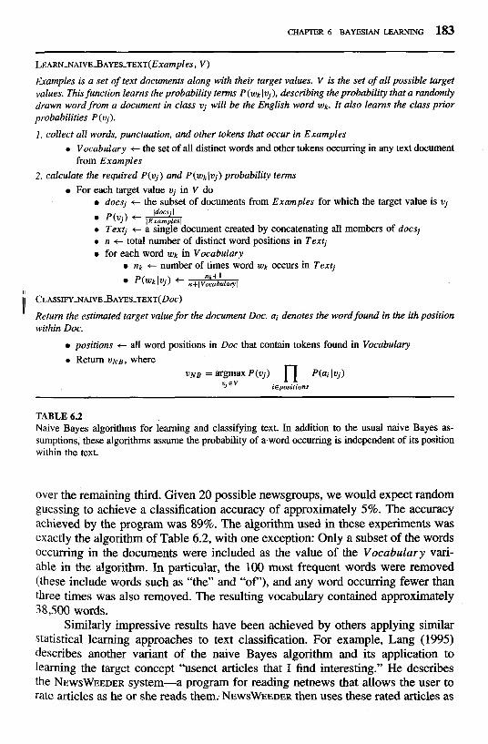
Examples is a set of text documents along with their target values. V is the set of all possible target values. This function learns the probability terms P(wk Iv,), describing the probability that a randomly drawn word from a document in class vj will be the English word wk. It also learns the class prior probabilities P(vj). 1. collect all words, punctwtion, and other tokens that occur in Examples
a Vocabulary c the set of all distinct words and other tokens occurring in any text document from Examples
2. calculate the required P(vj) and P(wkJvj) probability terms For each target value vj in V do
docsj t the subset of documents from Examples for which the target value is vj ldocs . I
P(uj) + 1ExornLlesl a Texti c a single document created by concatenating all members of docsi a n +*total number of distinct word positions in ~ e x c 0 for each word wk in Vocabulary
0 nk c number of times word wk occurs in Textj P(wk lvj) + n+12LLoryl
" Return the estimated target value for the document Doc. ai denotes the word found in the ith position within Doc.
0 positions t all word positions in Doc that contain tokens found in Vocabulary a Return V N B , where
V N B = argmax ~ ( v j ) n P(ai 19) V, E V ieposirions
TABLE 6.2 Naive Bayes algorithms for learning and classifying text. In addition to the usual naive Bayes as- sumptions, these algorithms assume the probability of a word occurring is independent of its position within the text.
over the remaining third. Given 20 possible newsgroups, we would expect random guessing to achieve a classification accuracy of approximately 5%. The accuracy achieved by the program was 89%. The algorithm used in these experiments was exactly the algorithm of Table 6.2, with one exception: Only a subset of the words occurring in the documents were included as the value of the Vocabulary vari- able in the algorithm. In particular, the 100 most frequent words were removed (these include words such as "the" and "of '), and any word occurring fewer than three times was also removed. The resulting vocabulary contained approximately 38,500 words.
Similarly impressive results have been achieved by others applying similar statistical learning approaches to text classification. For example, Lang (1995) describes another variant of the naive Bayes algorithm and its application to learning the target concept "usenet articles that I find interesting." He describes the NEWSWEEDER system-a program for reading netnews that allows the user to rate articles as he or she reads them. NEWSWEEDER then uses these rated articles as

TABLE 6.3 Twenty usenet newsgroups used in the text classification experiment. After training on 667 articles from each newsgroup, a naive Bayes classifier achieved an accuracy of 89% predicting to which newsgroup subsequent articles belonged. Random guessing would produce an accuracy of only 5%.
training examples to learn to predict which subsequent articles will be of interest to the user, so that it can bring these to the user's attention. Lang (1995) reports experiments in which NEWSWEEDER used its learned profile of user interests to suggest the most highly rated new articles each day. By presenting the user with the top 10% of its automatically rated new articles each day, it created a pool of articles containing three to four times as many interesting articles as the general pool of articles read by the user. For example, for one user the fraction of articles rated "interesting" was 16% overall, but was 59% among the articles recommended by NEWSWEEDER.
Several other, non-Bayesian, statistical text learning algorithms are common, many based on similarity metrics initially developed for information retrieval (e.g., see Rocchio 197 1; Salton 199 1). Additional text learning algorithms are described in Hearst and Hirsh (1996).
6.11 BAYESIAN BELIEF NETWORKS As discussed in the previous two sections, the naive Bayes classifier makes signif- icant use of the assumption that the values of the attributes a1 . . .a, are condition- ally independent given the target value v. This assumption dramatically reduces the complexity of learning the target function. When it is met, the naive Bayes classifier outputs the optimal Bayes classification. However, in many cases this conditional independence assumption is clearly overly restrictive.
A Bayesian belief network describes the probability distribution governing a set of variables by specifying a set of conditional independence assumptions along with a set of conditional probabilities. In contrast to the naive Bayes classifier, which assumes that all the variables are conditionally independent given the value of the target variable, Bayesian belief networks allow stating conditional indepen- dence assumptions that apply to subsets of the variables. Thus, Bayesian belief networks provide an intermediate approach that is less constraining than the global assumption of conditional independence made by the naive Bayes classifier, but more tractable than avoiding conditional independence assumptions altogether. Bayesian belief networks are an active focus of current research, and a variety of algorithms have been proposed for learning them and for using them for inference.
CHAPTER 6 BAYESIAN LEARNING 185
In this section we introduce the key concepts and the representation of Bayesian belief networks. More detailed treatments are given by Pearl (1988), Russell and Norvig (1995), Heckerman et al. (1995), and Jensen (1996).
In general, a Bayesian belief network describes the probability distribution over a set of variables. Consider an arbitrary set of random variables Yl . . . Y,, where each variable Yi can take on the set of possible values V(Yi). We define the joint space of the set of variables Y to be the cross product V(Yl) x V(Y2) x . . . V(Y,). In other words, each item in the joint space corresponds to one of the possible assignments of values to the tuple of variables (Yl . . . Y,). The probability distribution over this joint' space is called the joint probability distribution. The joint probability distribution specifies the probability for each of the possible variable bindings for the tuple (Yl . . . Y,). A Bayesian belief network describes the joint probability distribution for a set of variables.
6.11.1 Conditional Independence i Let us begin our discussion of Bayesian belief networks by defining precisely the notion of conditional independence. Let X , Y, and Z be three discrete-valued random variables. We say that X is conditionally independent of Y given Z if the probability distribution governing X is independent of the value of Y given a value for 2; that is, if
where xi E V(X), yj E V(Y), and z k E V(Z). We commonly write the above expression in abbreviated form as P(XIY, Z ) = P(X1Z). This definition of con- ditional independence can be extended to sets of variables as well. We say that the set of variables X1 . . . Xi is conditionally independent of the set of variables Yl . . . Ym given the set of variables 2 1 . . . Z, if
P ( X 1 ... XIJY1 ... Ym, z1 ... Z,) = P ( X l ... X1]Z1 ... Z,)
Note the correspondence between this definition and our use of conditional , independence in the definition of the naive Bayes classifier. The naive Bayes classifier assumes that the instance attribute A1 is conditionally independent of instance attribute A2 given the target value V. This allows the naive Bayes clas- sifier to calculate P ( A l , A21V) in Equation (6.20) as follows
Equation (6.23) is just the general form of the product rule of probability from Table 6.1. Equation (6.24) follows because if A1 is conditionally independent of A2 given V, then by our definition of conditional independence P (A1 IA2, V ) = P(A1IV).
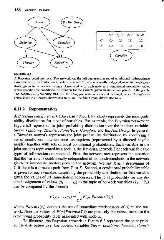
S,B S,-B 7S.B 1s.-B
-C 0.6 0.9 0.2
Campfire
FIGURE 6.3 A Bayesian belief network. The network on the left represents a set of conditional independence assumptions. In particular, each node is asserted to be conditionally independent of its nondescen- dants, given its immediate parents. Associated with each node is a conditional probability table, which specifies the conditional distribution for the variable given its immediate parents in the graph. The conditional probability table for the Campjire node is shown at the right, where Campjire is abbreviated to C, Storm abbreviated to S, and BusTourGroup abbreviated to B.
6.11.2 Representation A Bayesian belief network (Bayesian network for short) represents the joint prob- ability distribution for a set of variables. For example, the Bayesian network in Figure 6.3 represents the joint probability distribution over the boolean variables Storm, Lightning, Thunder, ForestFire, Campjre, and BusTourGroup. In general, a Bayesian network represents the joint probability distribution by specifying a set of conditional independence assumptions (represented by a directed acyclic graph), together with sets of local conditional probabilities. Each variable in the joint space is represented by a node in the Bayesian network. For each variable two types of information are specified. First, the network arcs represent the assertion that the variable is conditionally independent of its nondescendants in the network given its immediate predecessors in the network. We say Xjis a descendant of
, Y if there is a directed path from Y to X. Second, a conditional probability table is given for each variable, describing the probability distribution for that variable given the values of its immediate predecessors. The joint probability for any de- sired assignment of values (y l , . . . , y,) to the tuple of network variables (YI . . . Y,) can be computed by the formula
n
~ ( Y I , . . . , yd = n p ( y i ~ p a r e n t s ( ~ i ) ) i = l
where Parents(Yi) denotes the set of immediate predecessors of Yi in the net- work. Note the values of P(yiJ Parents(Yi)) are precisely the values stored in the conditional probability table associated with node Yi.
To illustrate, the Bayesian network in Figure 6.3 represents the joint prob- ability distribution over the boolean variables Storm, Lightning, Thunder, Forest-
C H m R 6 BAYESIAN LEARNING 187
Fire, Campfire, and BusTourGroup. Consider the node Campjire. The network nodes and arcs represent the assertion that CampJire is conditionally indepen- dent of its nondescendants Lightning and Thunder, given its immediate parents Storm and BusTourGroup. This means that once we know the value of the vari- ables Storm and BusTourGroup, the variables Lightning and Thunder provide no additional information about Campfire. The right side of the figure shows the conditional probability table associated with the variable Campfire. The top left entry in this table, for example, expresses the assertion that
P(Campfire = TruelStorm = True, BusTourGroup = True) = 0.4
Note this table provides only the conditional probabilities of Campjire given its parent variables Storm and BusTourGroup. The set of local conditional probability tables for all the variables, together with the set of conditional independence as- sumptions described by the network, describe the full joint probability distribution for the network.
One attractive feature of Bayesian belief networks is that they allow a con- venient way to represent causal knowledge such as the fact that Lightning causes Thunder. In the terminology of conditional independence, we express this by stat- ing that Thunder is conditionally independent of other variables in the network, given the value of Lightning. Note this conditional independence assumption is implied by the arcs in the Bayesian network of Figure 6.3.
6.11.3 Inference We might wish to use a Bayesian network to infer the value of some target variable (e.g., ForestFire) given the observed values of the other variables. Of course, given that we are dealing with random variables it will not generally be correct to assign the target variable a single determined value. What we really wish to infer is the probability distribution for the target variable, which specifies the probability that it will take on each of its possible values given the observed values of the other variables. This inference step can be straightforward if values for all of the other variables in the network are known exactly. In the more general case we may wish to infer the probability distribution for some variable (e.g., ForestFire) given observed values for only a subset of the other variables (e.g., Thunder and BusTourGroup may be the only observed values available). In general, a Bayesian network can be used to compute the probability distribution for any subset of network variables given the values or distributions for any subset of the remaining variables.
Exact inference of probabilities in general for an arbitrary Bayesian net- work is known to be NP-hard (Cooper 1990). Numerous methods have been proposed for probabilistic inference in Bayesian networks, including exact infer- ence methods and approximate inference methods that sacrifice precision to gain efficiency. For example, Monte Carlo methods provide approximate solutions by randomly sampling the distributions of the unobserved variables (Pradham and Dagum 1996). In theory, even approximate inference of probabilities in Bayesian
networks can be NP-hard (Dagum and Luby 1993). Fortunately, in practice ap- proximate methods have been shown to be useful in many cases. Discussions of inference methods for Bayesian networks are provided by Russell and Norvig (1995) and by Jensen (1996).
6.11.4 Learning Bayesian Belief Networks Can we devise effective algorithms for learning Bayesian belief networks from training data? This question is a focus of much current research. Several different settings for this learning problem can be considered. First, the network structure might be given in advance, or it might have to be inferred from the training data. Second, all the network variables might be directly observable in each training example, or some might be unobservable.
In the case where the network structure is given in advance and the variables are fully observable in the training examples, learning the conditional probability tables is straightforward. We simply estimate the conditional probability table entries just as we would for a naive Bayes classifier.
In the case where the network structure is given but only some of the variable values are observable in the training data, the learning problem is more difficult. This problem is somewhat analogous to learning the weights for the hidden units in an artificial neural network, where the input and output node values are given but the hidden unit values are left unspecified by the training examples. In fact, Russell et al. (1995) propose a similar gradient ascent procedure that learns the entries in the conditional probability tables. This gradient ascent procedure searches through a space of hypotheses that corresponds to the set of all possible entries for the conditional probability tables. The objective function that is maximized during gradient ascent is the probability P(D1h) of the observed training data D given the hypothesis h. By definition, this corresponds to searching for the maximum likelihood hypothesis for the table entries.
6.11.5 Gradient Ascent Training of Bayesian Networks The gradient ascent rule given by Russell et al. (1995) maximizes P(D1h) by following the gradient of In P(D Ih) with respect to the parameters that define the conditional probability tables of the Bayesian network. Let wi;k denote a single entry in one of the conditional probability tables. In particular, let wijk denote the conditional probability that the network variable Yi will take on the value yi, given that its immediate parents Ui take on the values given by uik. For example, if wijk is the top right entry in the conditional probability table in Figure 6.3, then Yi is the variable Campjire, Ui is the tuple of its parents (Stomz, BusTourGroup), yij = True, and uik = (False, False). The gradient of In P(D1h) is given by the derivatives for each of the toijk. As we show below, each of these derivatives can be calculated as
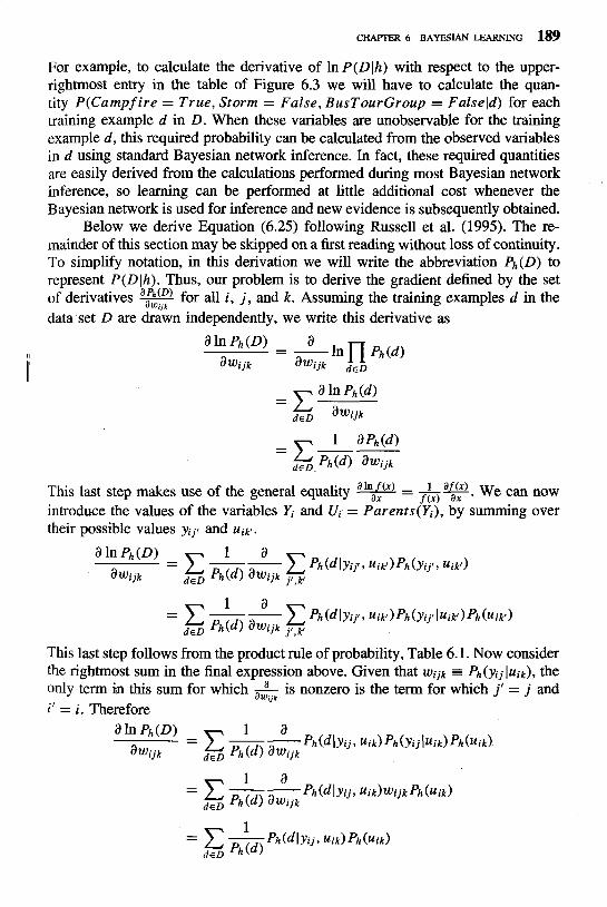
CHAPTER 6 BAYESIAN LEARNING 189
For example, to calculate the derivative of In P(D1h) with respect to the upper- rightmost entry in the table of Figure 6.3 we will have to calculate the quan- tity P(Campf ire = True, Storm = False, BusTourGroup = Falseld) for each training example d in D . When these variables are unobservable for the training example d , this required probability can be calculated from the observed variables in d using standard Bayesian network inference. In fact, these required quantities are easily derived from the calculations performed during most Bayesian network inference, so learning can be performed at little additional cost whenever the Bayesian network is used for inference and new evidence is subsequently obtained.
Below we derive Equation (6.25) following Russell et al. (1995). The re- mainder of this section may be skipped on a first reading without loss of continuity. To simplify notation, in this derivation we will write the abbreviation Ph(D) to represent P ( D J h ) . Thus, our problem is to derive the gradient defined by the set of derivatives for all i , j, and k . Assuming the training examples d in the data set D are drawn independently, we write this derivative as
This last step makes use of the general equality 9 = 1- f ( ~ ) ax . W can now introduce the values of the variables Yi and Ui = Parents(Yi) , by summing over their possible values yijl and uiu.
This last step follows from the product rule of probability, Table 6.1. Now consider the rightmost sum in the final expression above. Given that Wijk = Ph(yijl~ik), the only term in this sum for which & is nonzero is the term for which j' = j and i' = i . Therefore

Applying Bayes theorem to rewrite Ph (dlyi j , uik) , we have
Thus, we have derived the gradient given in Equation (6.25). There is one more item that must be considered before we can state the gradient ascent training procedure. In particular, we require that as the weights wijk are updated they must remain valid probabilities in the interval [0,1]. We also require that the sum xj wijk remains 1 for all i , k. These constraints can be satisfied by updating weights in a two-step process. First we update each wijk by gradient ascent
where q is a small constant called the learning rate. Second, we renormalize the weights wijk to assure that the above constraints are satisfied. As discussed by Russell et al., this process will converge to a locally maximum likelihood hypothesis for the conditional probabilities in the Bayesian network.
As in other gradient-based approaches, this algorithm is guaranteed only to find some local optimum solution. An alternative to gradient ascent is the EM algorithm discussed in Section 6.12, which also finds locally maximum likelihood solutions.
6.11.6 Learning the Structure of Bayesian Networks Learning Bayesian networks when the network structure is not known in advance is also difficult. Cooper and Herskovits (1992) present a Bayesian scoring metric for choosing among alternative networks. They also present a heuristic search algorithm called K2 for learning network structure when the data is fully observ- able. Like most algorithms for learning the structure of Bayesian networks, K2 performs a greedy search that trades off network complexity for accuracy over the training data. In one experiment K2 was given a set of 3,000 training examples generated at random from a manually constructed Bayesian network containing 37 nodes and 46 arcs. This particular network described potential anesthesia prob- lems in a hospital operating room. In addition to the data, the program was also given an initial ordering over the 37 variables that was consistent with the partial
CHAPTER 6 BAYESIAN LEARNING 191
ordering of variable dependencies in the actual network. The program succeeded in reconstructing the correct Bayesian network structure almost exactly, with the exception of one incorrectly deleted arc and one incorrectly added arc.
Constraint-based approaches to learning Bayesian network structure have also been developed (e.g., Spirtes et al. 1993). These approaches infer indepen- dence and dependence relationships from the data, and then use these relation- ships to construct Bayesian networks. Surveys of current approaches to learning Bayesian networks are provided by Heckerman (1995) and Buntine (1994).
6.12 THE EM ALGORITHM In many practical learning settings, only a subset of the relevant instance features might be observable. For example, in training or using the Bayesian belief network of Figure 6.3, we might have data where only a subset of the network variables Storm, Lightning, Thunder, ForestFire, Campfire, and BusTourGroup have been observed. Many approaches have been proposed to handle the problem of learning in the presence of unobserved variables. As we saw in Chapter 3, if some variable / is sometimes observed and sometimes not, then we can use the cases for which it has been observed to learn to predict its values when it is not. In this section we describe the EM algorithm (Dempster et al. 1977), a widely used approach to learning in the presence of unobserved variables. The EM algorithm can be used even for variables whose value is never directly observed, provided the general form of the probability distribution governing these variables is known. The EM algorithm has been used to train Bayesian belief networks (see Heckerman 1995) as well as radial basis function networks discussed in Section 8.4. The EM algorithm is also the basis for many unsupervised clustering algorithms (e.g., Cheeseman et al. 1988), and it is the basis for the widely used Baum-Welch forward-backward algorithm for learning Partially Observable Markov Models (Rabiner 1989).
6.12.1 Estimating Means of k Gaussians The easiest way to introduce the EM algorithm is via an example. Consider a problem in which the data D is a set of instances generated by a probability distribution that is a mixture of k distinct Normal distributions. This problem setting is illustrated in Figure 6.4 for the case where k = 2 and where the instances are the points shown along the x axis. Each instance is generated using a two-step process. First, one of the k Normal distributions is selected at random. Second, a single random instance xi is generated according to this selected distribution. This process is repeated to generate a set of data points as shown in the figure. To simplify our discussion, we consider the special case where the selection of the single Normal distribution at each step is based on choosing each with uniform probability, where each of the k Normal distributions has the same variance a2, and where a2 is known. The learning task is to output a hypothesis h = (FI, . . . pk) that describes the means of each of the k distributions. We would like to find
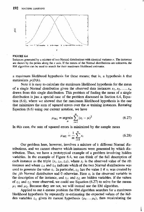
FIGURE 6.4 Instances generated by a mixture of two Normal distributions with identical variance a. The instances are shown by the points along the x axis. If the means of the Normal distributions are unknown, the EM algorithm can be used to search for their maximum likelihood estimates.
a maximum likelihood hypothesis for these means; that is, a hypothesis h that maximizes p ( D lh).
Note it is easy to calculate the maximum likelihood hypothesis for the mean of a single Normal distribution given the observed data instances XI, x2, . . . , xm drawn from this single distribution. This problem of finding the mean of a single distribution is just a special case of the problem discussed in Section 6.4, Equa- tion (6.6), where we showed that the maximum likelihood hypothesis is the one that minimizes the sum of squared errors over the m training instances. Restating Equation (6.6) using our current notation, we have
In this case, the sum of squared errors is minimized by the sample mean
Our problem here, however, involves a mixture of k different Normal dis- tributions, and we cannot observe which instances were generated by which dis- tribution. Thus, we have a prototypical example of a problem involving hidden variables. In the example of Figure 6.4, we can think of the full description of each instance as the triple (xi, zil , ziz), where xi is the observed value of the ith instance and where zil and zi2 indicate which of the two Normal distributions was used to generate the value xi. In particular, zij has the value 1 if xi was created by the jth Normal distribution and 0 otherwise. Here xi is the observed variable in the description of the instance, and zil and zi2 are hidden variables. If the values of zil and zi2 were observed, we could use Equation (6.27) to solve for the means p1 and p2. Because they are not, we will instead use the EM algorithm.
Applied to our k-means problem the EM algorithm searches for a maximum likelihood hypothesis by repeatedly re-estimating the expected values of the hid- den variables zij given its current hypothesis (pI . . . pk), then recalculating the
CHAPTER 6 BAYESIAN LEARNING 193
maximum likelihood hypothesis using these expected values for the hidden vari- ables. We will first describe this instance of the EM algorithm, and later state the EM algorithm in its general form.
'
Applied to the problem of estimating the two means for Figure 6.4, the EM algorithm first initializes the hypothesis to h = (PI, p2), where p1 and p2 are arbitrary initial values. It then iteratively re-estimates h by repeating the following two steps until the procedure converges to a stationary value for h.
Step 1: Calculate the expected value E[zi j ] of each hidden variable zi,, assuming the current hypothesis h = (p1, p2) holds.
Step 2: Calculate a new maximum likelihood hypothesis h' = (pi, p;), assuming the value taken on by each hidden variable zij is its expected value E[z i j ] calculated in Step 1. Then replace the hypothesis h = (pl, p2) by the new hypothesis h' = (pi, pi) and iterate.
Let us examine how both of these steps can be implemented in practice. / Step 1 must calculate the expected value of each zi,. This E [ 4 ] is just the prob- ability that instance xi was generated by the jth Normal distribution
Thus the first step is implemented by substituting the current values (pl, p2) and the observed xi into the above expression.
In the second step we use the E[zij] calculated during Step 1 to derive a new maximum likelihood hypothesis h' = (pi, pi). AS we will discuss later, the maximum likelihood hypothesis in this case is given by
Note this expression is similar to the sample mean from Equation (6.28) that is used to estimate p for a single Normal distribution. Our new expression is just the weighted sample mean for pj , with each instance weighted by the expectation E[z,j] that it was generated by the jth Normal distribution.
The above algorithm for estimating the means of a mixture of k Normal distributions illustrates the essence of the EM approach: The current hypothesis is used to estimate the unobserved variables, and the expected values of these variables are then used to calculate an improved hypothesis. It can be proved that on each iteration through this loop, the EM algorithm increases the likelihood P(Dlh) unless it is at a local maximum. The algorithm thus converges to a local maximum likelihood hypothesis for (pl, w2) .
6.12.2 General Statement of EM Algorithm Above we described an EM algorithm for the problem of estimating means of a mixture of Normal distributions. More generally, the EM algorithm can be applied in many settings where we wish to estimate some set of parameters 8 that describe an underlying probability distribution, given only the observed portion of the full data produced by this distribution. In the above two-means example the parameters of interest were 8 = (PI, p2), and the full data were the triples (xi, zil, zi2) of which only the xi were observed. In general let X = {xl, . . . , x,} denote the observed data in a set of m independently drawn instances, let Z = {zl, . . . , z,} denote the unobserved data in these same instances, and let Y = X U Z denote the full data. Note the unobserved Z can be treated as a random variable whose probability distribution depends on the unknown parameters 8 and on the observed data X. Similarly, Y is a random variable because it is defined in terms of the random variable Z. In the remainder of this section we describe the general form of the EM algorithm. We use h to denote the current hypothesized values of the parameters 8, and h' to denote the revised hypothesis that is estimated on each iteration of the EM algorithm.
The EM algorithm searches for the maximum likelihood hypothesis h' by seeking the h' that maximizes E[ln P(Y (h' ) ] . This expected value is taken over the probability distribution governing Y , which is determined by the unknown parameters 8. Let us consider exactly what this expression signifies. First, P(Ylhl) is the likelihood of the full data Y given hypothesis h'. It is reasonable that we wish to find a h' that maximizes some function of this quantity. Second, maximizing the logarithm of this quantity In P(Ylhl) also maximizes P(Ylhl) , as we have discussed on several occasions already. Third, we introduce the expected value E[ln P(Ylhl)] because the full data Y is itself a random variable. Given that the full data Y is a combination of the observed data X and unobserved data Z, we must average over the possible values of the unobserved Z, weighting each according to its probability. In other words we take the expected value E[ln P(Y lh')] over the probability distribution governing the random variable Y . The distribution governing Y is determined by the completely known values for X, plus the distribution governing Z.
What is the probability distribution governing Y ? In general we will not know this distribution because it is determined by the parameters 0 that we are trying to estimate. Therefore, the EM algorithm uses its current hypothesis h in place of the actual parameters 8 to estimate the distribution governing Y . Let us define a function Q(hllh) that gives E[ln P(Y lh')] as a function of h', under the assumption that 8 = h and given the observed portion X of the full data Y .
We write this function Q in the form Q(hllh) to indicate that it is defined in part by the assumption that the current hypothesis h is equal to 8. In its general form, the EM algorithm repeats the following two steps until convergence:
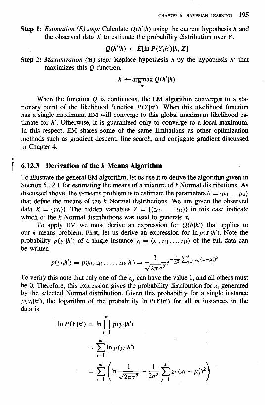
CHAPTER 6 BAYESIAN LEARNING 195
Step 1: Estimation (E) step: Calculate Q(hllh) using the current hypothesis h and the observed data X to estimate the probability distribution over Y .
Q(hf (h) t E[ln P(Ylhl)lh, XI Step 2: Maximization (M) step: Replace hypothesis h by the hypothesis h' that
maximizes this Q function. h t argmax Q (hf 1 h)
h'
When the function Q is continuous, the EM algorithm converges to a sta- tionary point of the likelihood function P(Y(h l ) . When this likelihood function has a single maximum, EM will converge to this global maximum likelihood es- timate for h'. Otherwise, it is guaranteed only to converge to a local maximum. In this respect, EM shares some of the same limitations as other optimization methods such as gradient descent, line search, and conjugate gradient discussed in Chapter 4.
11 6.12.3 Derivation of the k Means Algorithm To illustrate the general EM algorithm, let us use it to derive the algorithm given in Section 6.12.1 for estimating the means of a mixture of k Normal distributions. As discussed above, the k-means problem is to estimate the parameters 0 = ( P I . . . pk) that define the means of the k Normal distributions. We are given the observed data X = { ( x i ) } . The hidden variables Z = { ( z i l , . . . , z i k ) } in this case indicate which of the k Normal distributions was used to generate xi.
To apply EM we must derive an expression for Q(h(hf ) that applies to our k-means problem. First, let us derive an expression for 1np(Y(h1). Note the probability p(yi (h') of a single instance yi = (x i , Z i l , . . . ~ i k ) of the full data can be written
To verify this note that only one of the zij can have the value 1, and all others must be 0. Therefore, this expression gives the probability distribution for xi generated by the selected Normal distribution. Given this probability for a single instance p(yi(hl) , the logarithm of the probability In P(Y(hl) for all m instances in the data is
m
lnP(Ylhf) = l n n p ( , l h l ) i = l
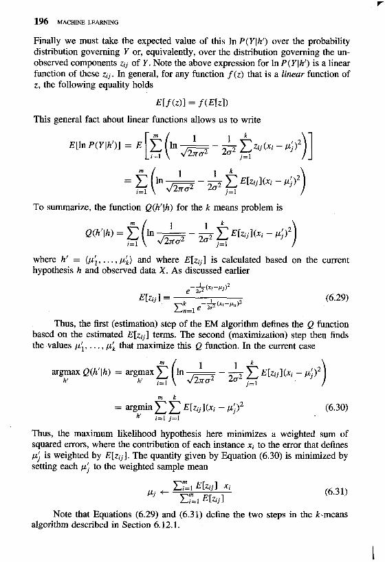
Finally we must take the expected value of this In P(Ylhl) over the probability distribution governing Y or, equivalently, over the distribution governing the un- observed components zij of Y. Note the above expression for In P(Ylhl) is a linear function of these zij. In general, for any function f (z) that is a linear function of z, the following equality holds
E[f (z)l = f (Ek.1) This general fact about linear functions allows us to write
To summarize, the function Q(hllh) for the k means problem is
where h' = (pi , . . . ,p i ) and where E[zij] is calculated based on the current hypothesis h and observed data X. As discussed earlier
e - & ( x ' - ~ ) 2
E[zij] = - --+ - - P " ) ~ (6.29)
EL1 e 2 Thus, the first (estimation) step of the EM algorithm defines the Q function
based on the estimated E[zij] terms. The second (maximization) step then finds the values pi, . . . , pi that maximize this Q function. In the current case
1 1 argmax Q(hllh) = argmax - - - h'
C E[zijI(xi - h1 i=l &2 2u2 j=l
Thus, the maximum likelihood hypothesis here minimizes a weighted sum of squared errors, where the contribution of each instance xi to the error that defines pj is weighted by E[zij]. The quantity given by Equation (6.30) is minimized by setting each pi to the weighted sample mean
Note that Equations (6.29) and (6.31) define the two steps in the k-means algorithm described in Section 6.12.1.
CHAPTER 6 BAYESIAN LEARNING 197
6.13 SUMMARY AND FURTHER READING The main points of this chapter include:
0 Bayesian methods provide the basis for probabilistic learning methods that accommodate (and require) knowledge about the prior probabilities of alter- native hypotheses and about the probability of observing various data given the hypothesis. Bayesian methods allow assigning a posterior probability to each candidate hypothesis, based on these assumed priors and the observed data.
0 Bayesian methods can be used to determine the most probable hypothesis given the data-the maximum a posteriori (MAP) hypothesis. This is the optimal hypothesis in the sense that no other hypothesis is more likely.
0 The Bayes optimal classifier combines the predictions of all alternative hy- potheses, weighted by their posterior probabilities, to calculate the most probable classification of each new instance.
i 0 The naive Bayes classifier is a Bayesian learning method that has been found to be useful in many practical applications. It is called "naive" because it in- corporates the simplifying assumption that attribute values are conditionally independent, given the classification of the instance. When this assumption is met, the naive Bayes classifier outputs the MAP classification. Even when this assumption is not met, as in the case of learning to classify text, the naive Bayes classifier is often quite effective. Bayesian belief networks pro- vide a more expressive representation for sets of conditional independence assumptions among subsets of the attributes.
0 The framework of Bayesian reasoning can provide a useful basis for ana- lyzing certain learning methods that do not directly apply Bayes theorem. For example, under certain conditions it can be shown that minimizing the squared error when learning a real-valued target function corresponds to computing the maximum likelihood hypothesis.
0 The Minimum Description Length principle recommends choosing the hy- pothesis that minimizes the description length of the hypothesis plus the description length of the data given the hypothesis. Bayes theorem and ba- sic results from information theory can be used to provide a rationale for this principle.
0 In many practical learning tasks, some of the relevant instance variables may be unobservable. The EM algorithm provides a quite general approach to learning in the presence of unobservable variables. This algorithm be- gins with an arbitrary initial hypothesis. It then repeatedly calculates the expected values of the hidden variables (assuming the current hypothesis is correct), and then recalculates the maximum likelihood hypothesis (as- suming the hidden variables have the expected values calculated by the first step). This procedure converges to a local maximum likelihood hypothesis, along with estimated values for the hidden variables.

There are many good introductory texts on probability and statistics, such as Casella and Berger (1990). Several quick-reference books (e.g., Maisel 1971; Speigel 1991) also provide excellent treatments of the basic notions of probability and statistics relevant to machine learning.
Many of the basic notions of Bayesian classifiers and least-squared error classifiers are discussed by Duda and Hart (1973). Domingos and Pazzani (1996) provide an analysis of conditions under which naive Bayes will output optimal classifications, even when its independence assumption is violated (the key here is that there are conditions under which it will output optimal classifications even when the associated posterior probability estimates are incorrect).
Cestnik (1990) provides a discussion of using the m-estimate to estimate probabilities.
Experimental results comparing various Bayesian approaches to decision tree learning and other algorithms can be found in Michie et al. (1994). Chauvin and Rumelhart (1995) provide a Bayesian analysis of neural network learning based on the BACKPROPAGATION algorithm.
A discussion of the Minimum Description Length principle can be found in Rissanen (1983, 1989). Quinlan and Rivest (1989) describe its use in avoiding overfitting in decision trees.
EXERCISES 6.1. Consider again the example application of Bayes rule in Section 6.2.1. Suppose the
doctor decides to order a second laboratory test for the same patient, and suppose the second test returns a positive result as well. What are the posterior probabilities of cancer and -cancer following these two tests? Assume that the two tests are independent.
6.2. In the example of Section 6.2.1 we computed the posterior probability of cancer by normalizing the quantities P (+(cancer) . P (cancer) and P (+I-cancer) . P (-cancer) so that they summed to one, Use Bayes theorem and the theorem of total probability (see Table 6.1) to prove that this method is valid (i.e., that normalizing in this way yields the correct value for P(cancerl+)).
6.3. Consider the concept learning algorithm FindG, which outputs a maximally general consistent hypothesis (e.g., some maximally general member of the version space). ( a ) Give a distribution for P(h) and P(D1h) under which FindG is guaranteed to
output a MAP hypothesis. (6) Give a distribution for P(h) and P(D1h) under which FindG is not guaranteed
to output a MAP .hypothesis. ( c ) Give a distribution for P(h) and P(D1h) under which FindG is guaranteed to
output a ML hypothesis but not a MAP hypothesis. 6.4. In the analysis of concept learning in Section 6.3 we assumed that the sequence of
instances (x l . . . x,) was held fixed. Therefore, in deriving an expression for P ( D ( h ) we needed only consider the probability of observing the sequence of target values ( d l . . . dm) for this fixed instance sequence. Consider the more general setting in which the instances are not held fixed, but are drawn independently from some probability distribution defined over the instance space X. The data D must now be described as the set of ordered pairs { ( x i , di)}, and P(D1h) must now reflect the

CHAPTER 6 BAYESIAN LEARNING 199
probability of encountering the specific instance X I , as well as the probability of the observed target value di. Show that Equation (6.5) holds even under this more general setting. Hint: Consider the analysis of Section 6.5.
6.5. Consider the Minimum Description Length principle applied to the hypothesis space H consisting of conjunctions of up to n boolean attributes (e.g., Sunny A Warm). Assume each hypothesis is encoded simply by listing the attributes present in the hypothesis, where the number of bits needed to encode any one of the n boolean at- tributes is log, n. Suppose the encoding of an example given the hypothesis uses zero bits if the example is consistent with the hypothesis and uses log, m bits otherwise (to indicate which of the m examples was misclassified-the correct classification can be inferred to be the opposite of that predicted by the hypothesis). ( a ) Write down the expression for the quantity to be minimized according to the
Minimum Description Length principle. (b) Is it possible to construct a set of training data such that a consistent hypothesis
exists, but MDL chooses a less consistent hypothesis? If so, give such a training set. If not, explain why not.
( c ) Give probability distributions for P ( h ) and P(D1h) such that the above MDL algorithm outputs MAP hypotheses.
6.6. Draw the Bayesian belief network that represents the conditional independence as- sumptions of the naive Bayes classifier for the PlayTennis problem of Section 6.9.1. Give the conditional probability table associated with the node Wind.
REFERENCES Buntine W. L. (1994). Operations for learning with graphical models. Journal of Art$cial Intelligence
Research, 2, 159-225. http://www.cs.washington.edu/research/jair/hom.html. Casella, G., & Berger, R. L. (1990). Statistical inference. Pacific Grove, CA: Wadsworth &
Brooks/Cole. Cestnik, B. (1990). Estimating probabilities: A crucial task in machine learning. Proceedings of the
Ninth European Conference on Am&5al Intelligence (pp. 147-149). London: Pitman. Chauvin, Y., & Rumelhart, D. (1995). Backpropagation: Theory, architectures, and applications,
(edited collection). Hillsdale, NJ: Lawrence Erlbaum Assoc. Cheeseman, P., Kelly, J., Self, M., Stutz, J., Taylor, W., & Freeman, D. (1988). AUTOCLASS: A
bayesian classification system. Proceedings of AAAI I988 (pp. 607-611). Cooper, G. (1990). Computational complexity of probabilistic inference using Bayesian belief net-
works (research note). Art@cial Intelligence, 42, 393-405. Cooper, G., & Herskovits, E. (1992). A Bayesian method for the induction of probabilistic networks
from data. Machine Learning, 9, 309-347. Dagum, P., & Luby, M. (1993). Approximating probabilistic reasoning in Bayesian belief networks
is NP-hard. Art$cial Intelligence, 60(1), 141-153. Dempster, A. P., Laird, N. M., & Rubin, D. B. (1977). Maximum likelihood from incomplete data
via the EM algorithm. Journal of the Royal Statistical Society, Series B, 39(1), 1-38. Domingos, P., & Pazzani, M. (1996). Beyond independence: Conditions for the optimality of the sim-
ple Bayesian classifier. Proceedings of the 13th International Conference on Machine Learning @p. 105-112).
Duda, R. O., & Hart, P. E. (1973). Pattern class$cation and scene analysis. New York: John Wiley & Sons.
Hearst, M., & Hirsh, H. (Eds.) (1996). Papers from the AAAI Spring Symposium on Machine Learning in Information Access, Stanford, March 25-27. http://www.parc.xerox.com/ist~ projects/mlia/
200 MACHINE LEARNING
Heckerman, D., Geiger, D., & Chickering, D. (1995) Learning Bayesian networks: The combination of knowledge and statistical data. Machine Learning, 20, 197. Kluwer Academic Publishers.
Jensen, F. V. (1996). An introduction to Bayesian networks. New York: Springer Verlag. Joachims, T. (1996). A probabilistic analysis of the Rocchio algorithm with TFIDF for text catego-
rization, (Computer Science Technical Report CMU-CS-96-118). Carnegie Mellon University. Lang, K. (1995). Newsweeder: Learning to filter netnews. In Prieditis and Russell (Eds.), Proceedings
of the 12th International Conference on Machine Learning (pp. 331-339). San Francisco: Morgan Kaufmann Publishers.
Lewis, D. (1991). Representation and learning in information retrieval, (Ph.D. thesis), (COINS Tech- nical Report 91-93). Dept. of Computer and Information Science, University of Massachusetts.
Madigan, D., & Rafferty, A. (1994). ~ o d e l selection and accounting for model uncertainty in graphi- cal models using Occam's window. Journal of the American Statistical Association, 89, 1535- 1546.
Maisel, L. (1971). Probability, statistics, and random processes. Simon and Schuster Tech Outlines. New York: Simon and Schuster.
Mehta, M., Rissanen, J., & Agrawal, R. (1995). MDL-based decision tree pruning. In U. M. Fayyard and R. Uthurusamy (Eds.), Proceedings of the First International Conference on Knowledge Discovery and Data Mining. Menlo Park, CA: AAAI Press.
Michie, D., Spiegelhalter, D. J., & Taylor, C. C. (1994). Machine learning, neural and statistical classification, (edited collection). New York: Ellis Horwood.
Opper, M., & Haussler, D. (1991). Generalization performance of Bayes optimal prediction algorithm for learning a perceptron. Physical Review Letters, 66, 2677-2681.
Pearl, J. (1988). Probabilistic reasoning in intelligent systems: Networks of plausible inference. San Mateo, CA: Morgan-Kaufmann.
Pradham, M., & Dagum, P. (1996). Optimal Monte Carlo estimation of belief network inference. In Proceedings of the Conference on Uncertainty in Artijicial Intelligence (pp. 44-53).
Quinlan, J. R., & Rivest, R. (1989). Inferring decision trees using the minimum description length principle. Information and Computation, 80, 227-248.
Rabiner, L. R. (1989). A tutorial on hidden Markov models and selected applications in speech recognition. Proceedings of the IEEE, 77(2), 257-286.
Rissanen, J. (1983). A universal prior for integers and estimation by minimum description length. The Annals of Statistics, 11(2), 41-31.
Rissanen, J., (1989). Stochastic complexity in statistical inquiry. New Jersey: World Scientific Pub. Rissanen, J. (1991). Information theory and neural nets. IBM Research Report RJ 8438 (76446),
IBM Thomas J. Watson Research Center, Yorktown Heights, NY. Rocchio, J. (1971). Relevance feedback in information retrieval. In The SMART retrieval system:
Experiments in automatic document processing, (Chap. 14, pp. 313-323). Englewood Cliffs, NJ: Prentice-Hall.
Russell, S., & Nomig, P. (1995). Artificial intelligence: A modem approach. Englewood Cliffs, NJ: Prentice-Hall.
Russell, S., Binder, J., Koller, D., & Kanazawa, K. (1995). Local learning in probabilistic networks with hidden variables. Proceedings of the 14th International Joint Conference on Artificial Intelligence, Montreal. San Francisco: Morgan Kaufmann.
Salton, G. (1991). Developments in automatic text retrieval. Science, 253, 974-979. Shannon, C. E., & Weaver, W. (1949). The mathematical theory of communication. Urbana: Univer-
sity of Illinois Press. Speigel, M. R. (1991). Theory and problems of probability and statistics. Schaum's Outline Series.
New York: McGraw Hill. Spirtes, P., Glymour, C., & Scheines, R. (1993). Causation, prediction, and search. New York:
Springer Verlag. http://hss.cmu.edu/htmUdepartments/philosophy~~D.BOO~ook.h~


![[PPT]PowerPoint Presentation - Swarthmore Collegeorgs.sccs.swarthmore.edu/swattank/files/2012/11/Final... · Web viewEliot Ingram - Background Swarthmore College, Econ/PoliSci double](https://img.pdfslide.us/doc/110x75/5abfe0e17f8b9add5f8e4712/pptpowerpoint-presentation-swarthmore-vieweliot-ingram-background-swarthmore.jpg)