5.1

1

CHAPTER 5

MEASURING RETURN ON INVESTMENTS

In Chapter 4, we developed a process for estimating costs of equity, debt, and

capital and presented an argument that the cost of capital is the minimum acceptable

hurdle rate when considering new investments. We also argued that an investment has to

earn a return greater than this hurdle rate to create value for the owners of a business. In

this chapter, we turn to the question of how best to measure the return on a project. In

doing so, we will attempt to answer the following questions:

• What is a project? In particular, how general is the definition of an investment and

what are the different types of investment decisions that firms have to make?

• In measuring the return on a project, should we look at the cash flows generated by

the project or at the accounting earnings?

• If the returns on a project are unevenly spread over time, how do we consider (or

should we not consider) differences in returns across time?

We will illustrate the basics of investment analysis using four hypothetical projects: an

online book ordering service for Bookscape, a new theme park in Brazil for Disney, a

plant to manufacture linerboard for Aracruz Celulose and an acquisition of a US

company by Tata Chemicals.

What Is a Project? Investment analysis concerns which projects a company should accept and which

it should reject; accordingly, the question of what makes up a project is central to this and

the following chapters. The conventional project

analyzed in capital budgeting has three criteria: (1)

a large up-front cost, (2) cash flows for a specific

time period, and (3) a salvage value at the end,

which captures the value of the assets of the project when the project ends. Although such

projects undoubtedly form a significant proportion of investment decisions, especially for

manufacturing firms, it would be a mistake to assume that investment analysis stops

there. If a project is defined more broadly to include any decision that results in using the

Salvage Value: The estimated liquidation

value of the assets invested in the projects

at the end of the project life.

5.2

2

scarce resources of a business, then everything from strategic decisions and acquisitions

to decisions about which air conditioning system to use in a building would fall within its

reach.

Defined broadly then, any of the following decisions would qualify as projects:

1. Major strategic decisions to enter new areas of business (such as Disney’s foray into

real estate or Deutsche Bank’s into investment banking) or new markets (such as

Disney television’s expansion into Latin America).

2. Acquisitions of other firms are projects as well, notwithstanding attempts to create

separate sets of rules for them.

3. Decisions on new ventures within existing businesses or markets, such as the one

made by Disney to expand its Orlando theme park to include the Animal Kingdom or

the decision to produce a new animated movie.

4. Decisions that may change the way existing ventures and projects are run, such as

programming schedules on the Disney channel or changing inventory policy at

Bookscape.

5. Decisions on how best to deliver a service that is necessary for the business to run

smoothly. A good example would be Deutsche Bank’s choice of what type of

financial information system to acquire to allow traders and investment bankers to do

their jobs. While the information system itself might not deliver revenues and profits,

it is an indispensable component for other

revenue generating projects.

Investment decisions can be categorized

on a number of different dimensions. The first

relates to how the project affects other projects

the firm is considering and analyzing. Some

projects are independent of other projects, and thus can be analyzed separately, whereas

other projects are mutually exclusive—that is, taking one project will mean rejecting

other projects. At the other extreme, some projects are prerequisites for other projects

down the road and others are complementary. In general, projects can be categorized as

falling somewhere on the continuum between prerequisites and mutually exclusive, as

depicted in Figure 5.1.

Mutually Exclusive Projects: A group

of projects is said to be mutually

exclusive when acceptance of one of the

projects implies that the rest have to be

rejected.

5.3

3

Figure 5.1 The Project Continuum

The second dimension that can be used to classify a project is its ability to

generate revenues or reduce costs. The decision rules that analyze revenue-generating

projects attempt to evaluate whether the earnings or cash flows from the projects justify

the investment needed to implement them. When it comes to cost-reduction projects, the

decision rules examine whether the reduction in costs justifies the up-front investment

needed for the projects.

Illustration 5.1: Project Descriptions.

In this chapter and parts of the next, we will use four hypothetical projects to

illustrate the basics of investment analysis.

• The first project we will look at is a proposal by Bookscape to add an online book

ordering and information service. Although the impetus for this proposal comes from

the success of other online retailers like Amazon.com, Bookscape’s service will be

more focused on helping customers research books and find the ones they need rather

than on price. Thus, if Bookscape decides to add this service, it will have to hire and

train well-qualified individuals to answer customer queries, in addition to investing in

the computer equipment and phone lines that the service will require. This project

analysis will help illustrate some of the issues that come up when private businesses

look at investments and also when businesses take on projects that have risk profiles

different from their existing ones.

• The second project we will analyze is a proposed theme park for Disney in Rio De

Janeiro, Brazil. Rio Disneyworld, which will be patterned on Disneyland Paris and

Walt Disney World in Florida, will require a huge investment in infrastructure and

take several years to complete. This project analysis will bring several issues to the

forefront, including questions of how to deal with projects when the cash flows are in

a foreign currency and what to do when projects have very long lives.

5.4

4

• The third project we will consider is a plant in Brazil to manufacture linerboard for

Aracruz Celulose. Linerboard is a stiffened paper product that can be transformed

into cardboard boxes. This investment is a more conventional one, with an initial

investment, a fixed lifetime, and a salvage value at the end. We will, however, do the

analysis for this project from an equity standpoint to illustrate the generality of

investment analysis. In addition, in light of concerns about inflation in Brazil, we will

do the analysis entirely in real terms.

• The final project that we will examine is Tata Chemical’s proposed acquisition of

Sensient Technologies, a publicly traded US firm that manufactures color, flavor and

fragrance additives for the food business. We will extend the same principles that we

use to value internal investments to analyze how much Tata Chemicals can afford to

pay for the US company and the value of any potential synergies in the merger.

We should also note that while these projects are hypothetical, they are based upon real

projects that these firms have taken in the past.

Hurdle Rates for Firms versus Hurdle Rates for Projects In the previous chapter we developed a process for estimating the costs of equity

and capital for firms. In this chapter, we will extend the discussion to hurdle rates in the

context of new or individual investments.

Using the Firm’s Hurdle Rate for Individual Projects Can we use the costs of equity and capital that we have estimated for the firms for

these projects? In some cases we can, but only if all investments made by a firm are

similar in terms of their risk exposure. As a firm’s investments become more diverse, the

firm will no longer be able to use its cost of equity and capital to evaluate these projects.

Projects that are riskier have to be assessed using a higher cost of equity and capital than

projects that are safer. In this chapter, we consider how to estimate project costs of equity

and capital.

What would happen if a firm chose to use its cost of equity and capital to evaluate

all projects? This firm would find itself overinvesting in risky projects and under

investing in safe projects. Over time, the firm will become riskier, as its safer businesses

find themselves unable to compete with riskier businesses.

5.5

5

Cost of Equity for Projects In assessing the beta for a project, we will consider three possible scenarios. The

first scenario is the one where all the projects considered by a firm are similar in their

exposure to risk; this homogeneity makes risk assessment simple. The second scenario is

one in which a firm is in multiple businesses with different exposures to risk, but projects

within each business have the same risk exposure. The third scenario is the most

complicated wherein each project considered by a firm has a different exposure to risk.

1. Single Business; Project Risk Similar within Business

When a firm operates in only one business and all projects within that business

share the same risk profile, the firm can use its overall cost of equity as the cost of equity

for the project. Because we estimated the cost of equity using a beta for the firm in

Chapter 4, this would mean that we would use the same beta to estimate the cost of equity

for each project that the firm analyzes. The advantage of this approach is that it does not

require risk estimation prior to every project, providing managers with a fixed benchmark

for their project investments. The approach is restricting, though, because it can be

usefully applied only to companies that are in one line of business and take on

homogeneous projects.

2. Multiple Businesses with Different Risk Profiles: Project Risk Similar within Each

Business

When firms operate in more than one line of business, the risk profiles are likely

to be different across different businesses. If we make the assumption that projects taken

within each business have the same risk profile, we can estimate the cost of equity for

each business separately and use that cost of equity for all projects within that business.

Riskier businesses will have higher costs of equity than safer businesses, and projects

taken by riskier businesses will have to cover these higher costs. Imposing the firm’s cost

of equity on all projects in all businesses will lead to overinvesting in risky businesses

(because the cost of equity will be set too low) and under investing in safe businesses

(because the cost of equity will be set too high).

How do we estimate the cost of equity for individual businesses? When the

approach requires equity betas, we cannot fall back on the conventional regression

5.6

6

approach (in the CAPM) or factor analysis (in the APM) because these approaches

require past prices. Instead, we have to use one of the two approaches that we described

in the last section as alternatives to regression betas—bottom-up betas based on other

publicly traded firms in the same business, or accounting betas, estimated based on the

accounting earnings for the division.

3. Projects with Different Risk Profiles

As a purist, you could argue that each project’s risk profile is, in fact, unique and that

it is inappropriate to use either the firm’s cost of equity or divisional costs of equity to

assess projects. Although this may be true, we have to consider the trade-off. Given that

small differences in the cost of equity should not make a significant difference in our

investment decisions, we have to consider whether the added benefits of analyzing each

project individually exceed the costs of doing so.

When would it make sense to assess a project’s risk individually? If a project is large

in terms of investment needs relative to the firm assessing it and has a very different risk

profile from other investments in the firm, it would make sense to assess the cost of

equity for the project independently. The only practical way of estimating betas and costs

of equity for individual projects is the bottom-up beta approach.

Cost of Debt for Projects

In the previous chapter, we noted that the cost of debt for a firm should reflect its

default risk. With individual projects, the assessment of default risk becomes much more

difficult, because projects seldom borrow on their own; most firms borrow money for all

the projects that they undertake. There are three approaches to estimating the cost of debt

for a project:

• One approach is based on the argument that because the borrowing is done by the

firm rather than by individual projects, the cost of debt for a project should be the

cost of debt for the firm considering the project. This approach makes the most

sense when the projects being assessed are small relative to the firm taking them

and thus have little or no appreciable effect on the firm’s default risk.

• Look at the project’s capacity to generate cash flows relative to its financing costs

and estimate default risk and cost of debt for the project, You can also estimate

5.7

7

this default risk by looking at other firms that take similar projects, and use the

typical default risk and cost of debt for these firms. This approach generally

makes sense when the project is large in terms of its capital needs relative to the

firm and has different cash flow characteristics (both in terms of magnitude and

volatility) from other investments taken by the firm and is capable of borrowing

funds against its own cash flows.

• The third approach applies when a project actually borrows its own funds, with

lenders having no recourse against the parent firm, in case the project defaults.

This is unusual, but it can occur when investments have significant tangible assets

of their own and the investment is large relative to the firm considering it. In this

case, the cost of debt for the project can be assessed using its capacity to generate

cash flows relative to its financing obligations. In the last chapter, we used the

bond rating of a firm to come up with the cost of debt for the firm. Although

projects may not be rated, we can still estimate a rating for a project based on

financial ratios, and this can be used to estimate default risk and the cost of debt.

Financing Mix and Cost of Capital for Projects To get from the costs of debt and equity to the cost of capital, we have to weight

each by their relative proportions in financing. Again, the task is much easier at the firm

level, where we use the current market values of debt and equity to arrive at these

weights. We may borrow money to fund a project, but it is often not clear whether we are

using the debt capacity of the project or the firm’s debt capacity. The solution to this

problem will again vary depending on the scenario we face.

• When we are estimating the financing weights for small projects that do not affect

a firm’s debt capacity, the financing weights should be those of the firm before

the project.

• When assessing the financing weights of large projects, with risk profiles different

from that of the firm, we have to be more cautious. Using the firm’s financing

mix to compute the cost of capital for these projects can be misleading, because

the project being analyzed may be riskier than the firm as a whole and thus

incapable of carrying the firm’s debt ratio. In this case, we would argue for the

5.8

8

use of the average debt ratio of the other firms in the business in assessing the cost

of capital of the project.

• The financing weights for stand-alone projects that are large enough to issue their

own debt should be based on the actual amounts borrowed by the projects. For

firms with such projects, the financing weights can vary from project to projects,

as will the cost of debt.

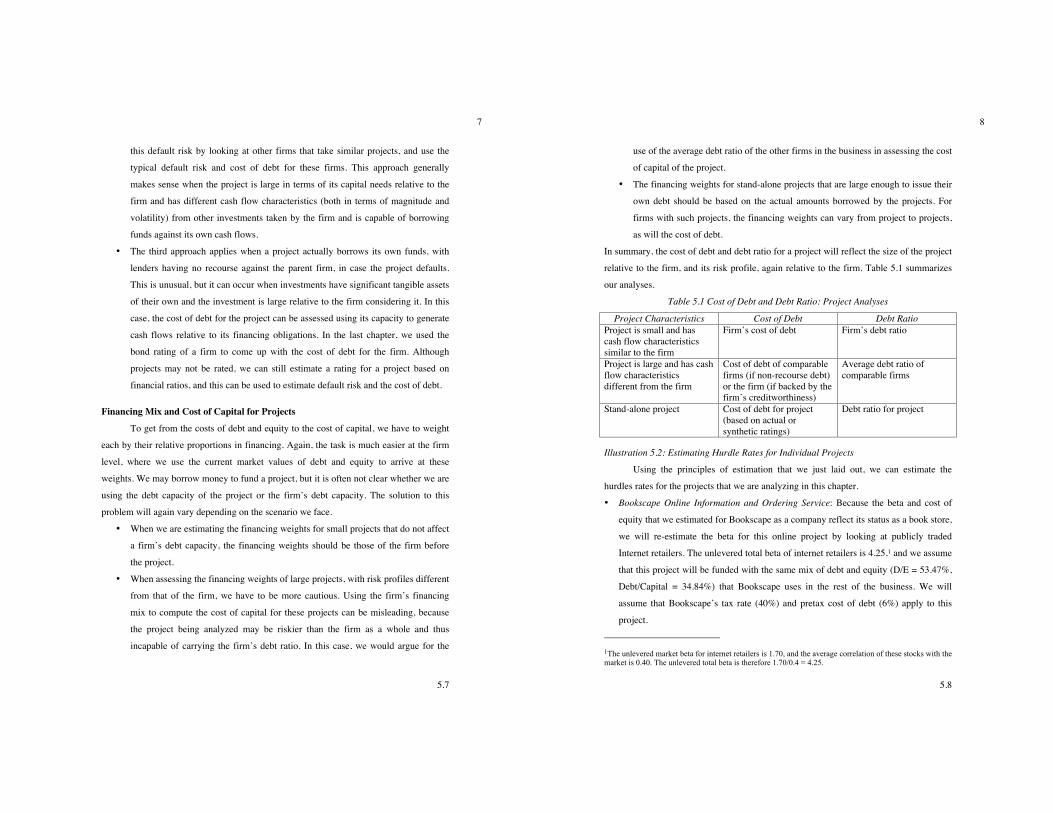
In summary, the cost of debt and debt ratio for a project will reflect the size of the project

relative to the firm, and its risk profile, again relative to the firm. Table 5.1 summarizes

our analyses.

Table 5.1 Cost of Debt and Debt Ratio: Project Analyses

Project Characteristics Cost of Debt Debt Ratio Project is small and has cash flow characteristics similar to the firm

Firm’s cost of debt Firm’s debt ratio

Project is large and has cash flow characteristics different from the firm

Cost of debt of comparable firms (if non-recourse debt) or the firm (if backed by the firm’s creditworthiness)

Average debt ratio of comparable firms

Stand-alone project Cost of debt for project (based on actual or synthetic ratings)

Debt ratio for project

Illustration 5.2: Estimating Hurdle Rates for Individual Projects

Using the principles of estimation that we just laid out, we can estimate the

hurdles rates for the projects that we are analyzing in this chapter.

• Bookscape Online Information and Ordering Service: Because the beta and cost of

equity that we estimated for Bookscape as a company reflect its status as a book store,

we will re-estimate the beta for this online project by looking at publicly traded

Internet retailers. The unlevered total beta of internet retailers is 4.25,1 and we assume

that this project will be funded with the same mix of debt and equity (D/E = 53.47%,

Debt/Capital = 34.84%) that Bookscape uses in the rest of the business. We will

assume that Bookscape’s tax rate (40%) and pretax cost of debt (6%) apply to this

project.

1The unlevered market beta for internet retailers is 1.70, and the average correlation of these stocks with the market is 0.40. The unlevered total beta is therefore 1.70/0.4 = 4.25.

5.9

9

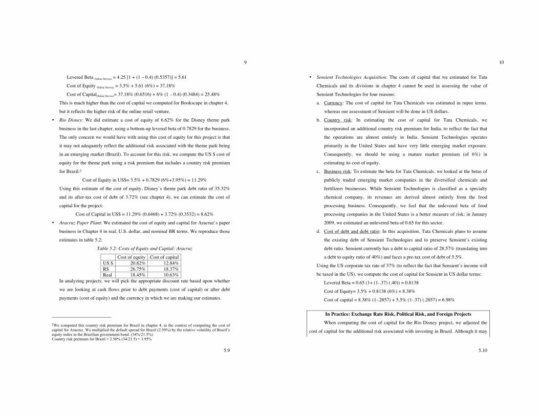
Levered Beta Online Service = 4.25 [1 + (1 – 0.4) (0.5357)] = 5.61

Cost of Equity Online Service = 3.5% + 5.61 (6%) = 37.18%

Cost of CapitalOnline Service= 37.18% (0.6516) + 6% (1 – 0.4) (0.3484) = 25.48%

This is much higher than the cost of capital we computed for Bookscape in chapter 4,

but it reflects the higher risk of the online retail venture.

• Rio Disney: We did estimate a cost of equity of 6.62% for the Disney theme park

business in the last chapter, using a bottom-up levered beta of 0.7829 for the business.

The only concern we would have with using this cost of equity for this project is that

it may not adequately reflect the additional risk associated with the theme park being

in an emerging market (Brazil). To account for this risk, we compute the US $ cost of

equity for the theme park using a risk premium that includes a country risk premium

for Brazil:2

Cost of Equity in US$= 3.5% + 0.7829 (6%+3.95%) = 11.29%

Using this estimate of the cost of equity, Disney’s theme park debt ratio of 35.32%

and its after-tax cost of debt of 3.72% (see chapter 4), we can estimate the cost of

capital for the project:

Cost of Capital in US$ = 11.29% (0.6468) + 3.72% (0.3532) = 8.62%

• Aracruz Paper Plant: We estimated the cost of equity and capital for Aracruz’s paper

business in Chapter 4 in real, U.S. dollar, and nominal BR terms. We reproduce those

estimates in table 5.2:

Table 5.2: Costs of Equity and Capital: Aracruz

Cost of equity Cost of capital US $ 20.82% 12.84% R$ 26.75% 18.37% Real 18.45% 10.63%

In analyzing projects, we will pick the appropriate discount rate based upon whether

we are looking at cash flows prior to debt payments (cost of capital) or after debt

payments (cost of equity) and the currency in which we are making our estimates.

2We computed this country risk premium for Brazil in chapter 4, in the context of computing the cost of capital for Aracruz. We multiplied the default spread for Brazil (2.50%) by the relative volatility of Brazil’s equity index to the Brazilian government bond. (34%/21.5%) Country risk premium for Brazil = 2.50% (34/21.5) = 3.95%

5.10

10

• Sensient Technologies Acquisition: The costs of capital that we estimated for Tata

Chemicals and its divisions in chapter 4 cannot be used in assessing the value of

Sensient Technologies for four reasons:

a. Currency: The cost of capital for Tata Chemicals was estimated in rupee terms,

whereas our assessment of Sensient will be done in US dollars.

b. Country risk: In estimating the cost of capital for Tata Chemicals, we

incorporated an additional country risk premium for India, to reflect the fact that

the operations are almost entirely in India. Sensient Technologies operates

primarily in the United States and have very little emerging market exposure.

Consequently, we should be using a mature market premium (of 6%) in

estimating its cost of equity.

c. Business risk: To estimate the beta for Tata Chemicals, we looked at the betas of

publicly traded emerging market companies in the diversified chemicals and

fertilizers businesses. While Sensient Technologies is classified as a specialty

chemical company, its revenues are derived almost entirely from the food

processing business. Consequently, we feel that the unlevered beta of food

processing companies in the United States is a better measure of risk; in January

2009, we estimated an unlevered beta of 0.65 for this sector.

d. Cost of debt and debt ratio: In this acquisition, Tata Chemicals plans to assume

the existing debt of Sensient Technologies and to preserve Sensient’s existing

debt ratio. Sensient currently has a debt to capital ratio of 28.57% (translating into

a debt to equity ratio of 40%) and faces a pre-tax cost of debt of 5.5%.

Using the US corporate tax rate of 37% (to reflect the fact that Sensient’s income will

be taxed in the US), we compute the cost of capital for Sensient in US dollar terms:

Levered Beta = 0.65 (1+ (1-.37) (.40)) = 0.8138

Cost of Equity= 3.5% + 0.8138 (6%) = 8.38%

Cost of capital = 8.38% (1-.2857) + 5.5% (1-.37) (.2857) = 6.98%

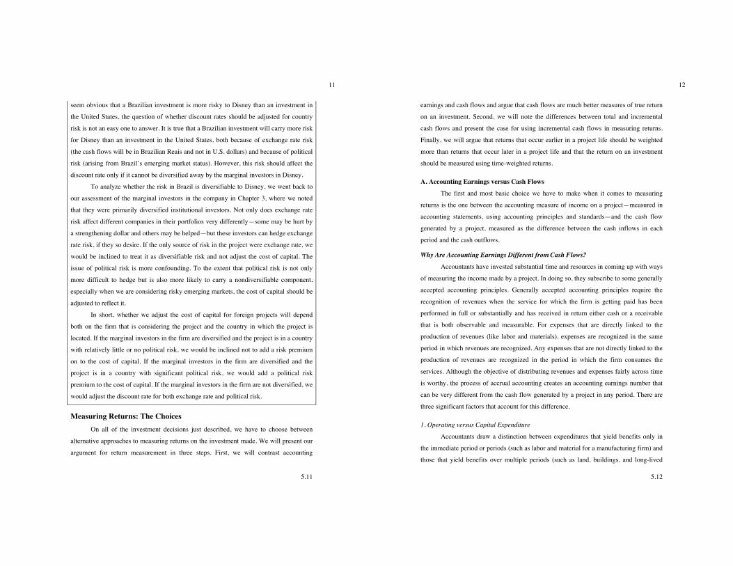
In Practice: Exchange Rate Risk, Political Risk, and Foreign Projects When computing the cost of capital for the Rio Disney project, we adjusted the

cost of capital for the additional risk associated with investing in Brazil. Although it may

5.11

11

seem obvious that a Brazilian investment is more risky to Disney than an investment in

the United States, the question of whether discount rates should be adjusted for country

risk is not an easy one to answer. It is true that a Brazilian investment will carry more risk

for Disney than an investment in the United States, both because of exchange rate risk

(the cash flows will be in Brazilian Reais and not in U.S. dollars) and because of political

risk (arising from Brazil’s emerging market status). However, this risk should affect the

discount rate only if it cannot be diversified away by the marginal investors in Disney.

To analyze whether the risk in Brazil is diversifiable to Disney, we went back to

our assessment of the marginal investors in the company in Chapter 3, where we noted

that they were primarily diversified institutional investors. Not only does exchange rate

risk affect different companies in their portfolios very differently—some may be hurt by

a strengthening dollar and others may be helped—but these investors can hedge exchange

rate risk, if they so desire. If the only source of risk in the project were exchange rate, we

would be inclined to treat it as diversifiable risk and not adjust the cost of capital. The

issue of political risk is more confounding. To the extent that political risk is not only

more difficult to hedge but is also more likely to carry a nondiversifiable component,

especially when we are considering risky emerging markets, the cost of capital should be

adjusted to reflect it.

In short, whether we adjust the cost of capital for foreign projects will depend

both on the firm that is considering the project and the country in which the project is

located. If the marginal investors in the firm are diversified and the project is in a country

with relatively little or no political risk, we would be inclined not to add a risk premium

on to the cost of capital. If the marginal investors in the firm are diversified and the

project is in a country with significant political risk, we would add a political risk

premium to the cost of capital. If the marginal investors in the firm are not diversified, we

would adjust the discount rate for both exchange rate and political risk.

Measuring Returns: The Choices On all of the investment decisions just described, we have to choose between

alternative approaches to measuring returns on the investment made. We will present our

argument for return measurement in three steps. First, we will contrast accounting

5.12

12

earnings and cash flows and argue that cash flows are much better measures of true return

on an investment. Second, we will note the differences between total and incremental

cash flows and present the case for using incremental cash flows in measuring returns.

Finally, we will argue that returns that occur earlier in a project life should be weighted

more than returns that occur later in a project life and that the return on an investment

should be measured using time-weighted returns.

A. Accounting Earnings versus Cash Flows The first and most basic choice we have to make when it comes to measuring

returns is the one between the accounting measure of income on a project—measured in

accounting statements, using accounting principles and standards—and the cash flow

generated by a project, measured as the difference between the cash inflows in each

period and the cash outflows.

Why Are Accounting Earnings Different from Cash Flows?

Accountants have invested substantial time and resources in coming up with ways

of measuring the income made by a project. In doing so, they subscribe to some generally

accepted accounting principles. Generally accepted accounting principles require the

recognition of revenues when the service for which the firm is getting paid has been

performed in full or substantially and has received in return either cash or a receivable

that is both observable and measurable. For expenses that are directly linked to the

production of revenues (like labor and materials), expenses are recognized in the same

period in which revenues are recognized. Any expenses that are not directly linked to the

production of revenues are recognized in the period in which the firm consumes the

services. Although the objective of distributing revenues and expenses fairly across time

is worthy, the process of accrual accounting creates an accounting earnings number that

can be very different from the cash flow generated by a project in any period. There are

three significant factors that account for this difference.

1. Operating versus Capital Expenditure

Accountants draw a distinction between expenditures that yield benefits only in

the immediate period or periods (such as labor and material for a manufacturing firm) and

those that yield benefits over multiple periods (such as land, buildings, and long-lived

5.13

13

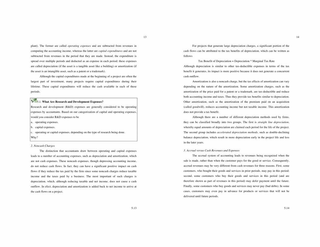
plant). The former are called operating expenses and are subtracted from revenues in

computing the accounting income, whereas the latter are capital expenditures and are not

subtracted from revenues in the period that they are made. Instead, the expenditure is

spread over multiple periods and deducted as an expense in each period; these expenses

are called depreciation (if the asset is a tangible asset like a building) or amortization (if

the asset is an intangible asset, such as a patent or a trademark).

Although the capital expenditures made at the beginning of a project are often the

largest part of investment, many projects require capital expenditures during their

lifetime. These capital expenditures will reduce the cash available in each of these

periods.

5.1. What Are Research and Development Expenses?

Research and development (R&D) expenses are generally considered to be operating

expenses by accountants. Based on our categorization of capital and operating expenses,

would you consider R&D expenses to be

a. operating expenses.

b. capital expenses.

c. operating or capital expenses, depending on the type of research being done.

Why?

2. Noncash Charges

The distinction that accountants draw between operating and capital expenses

leads to a number of accounting expenses, such as depreciation and amortization, which

are not cash expenses. These noncash expenses, though depressing accounting income,

do not reduce cash flows. In fact, they can have a significant positive impact on cash

flows if they reduce the tax paid by the firm since some noncash charges reduce taxable

income and the taxes paid by a business. The most important of such charges is

depreciation, which, although reducing taxable and net income, does not cause a cash

outflow. In efect, depreciation and amortization is added back to net income to arrive at

the cash flows on a project.

5.14

14

For projects that generate large depreciation charges, a significant portion of the

cash flows can be attributed to the tax benefits of depreciation, which can be written as

follows

Tax Benefit of Depreciation = Depreciation * Marginal Tax Rate

Although depreciation is similar to other tax-deductible expenses in terms of the tax

benefit it generates, its impact is more positive because it does not generate a concurrent

cash outflow.

Amortization is also a noncash charge, but the tax effects of amortization can vary

depending on the nature of the amortization. Some amortization charges, such as the

amortization of the price paid for a patent or a trademark, are tax-deductible and reduce

both accounting income and taxes. Thus they provide tax benefits similar to depreciation.

Other amortization, such as the amortization of the premium paid on an acquisition

(called goodwill), reduces accounting income but not taxable income. This amortization

does not provide a tax benefit.

Although there are a number of different depreciation methods used by firms,

they can be classified broadly into two groups. The first is straight line depreciation,

whereby equal amounts of depreciation are claimed each period for the life of the project.

The second group includes accelerated depreciation methods, such as double-declining

balance depreciation, which result in more depreciation early in the project life and less

in the later years.

3. Accrual versus Cash Revenues and Expenses

The accrual system of accounting leads to revenues being recognized when the

sale is made, rather than when the customer pays for the good or service. Consequently,

accrual revenues may be very different from cash revenues for three reasons. First, some

customers, who bought their goods and services in prior periods, may pay in this period;

second, some customers who buy their goods and services in this period (and are

therefore shown as part of revenues in this period) may defer payment until the future.

Finally, some customers who buy goods and services may never pay (bad debts). In some

cases, customers may even pay in advance for products or services that will not be

delivered until future periods.

5.15

15

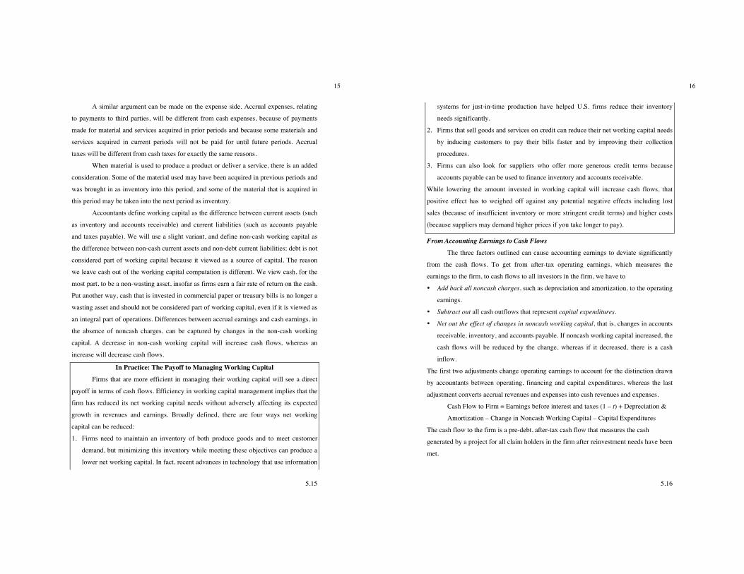
A similar argument can be made on the expense side. Accrual expenses, relating

to payments to third parties, will be different from cash expenses, because of payments

made for material and services acquired in prior periods and because some materials and

services acquired in current periods will not be paid for until future periods. Accrual

taxes will be different from cash taxes for exactly the same reasons.

When material is used to produce a product or deliver a service, there is an added

consideration. Some of the material used may have been acquired in previous periods and

was brought in as inventory into this period, and some of the material that is acquired in

this period may be taken into the next period as inventory.

Accountants define working capital as the difference between current assets (such

as inventory and accounts receivable) and current liabilities (such as accounts payable

and taxes payable). We will use a slight variant, and define non-cash working capital as

the difference between non-cash current assets and non-debt current liabilities; debt is not

considered part of working capital because it viewed as a source of capital. The reason

we leave cash out of the working capital computation is different. We view cash, for the

most part, to be a non-wasting asset, insofar as firms earn a fair rate of return on the cash.

Put another way, cash that is invested in commercial paper or treasury bills is no longer a

wasting asset and should not be considered part of working capital, even if it is viewed as

an integral part of operations. Differences between accrual earnings and cash earnings, in

the absence of noncash charges, can be captured by changes in the non-cash working

capital. A decrease in non-cash working capital will increase cash flows, whereas an

increase will decrease cash flows.

In Practice: The Payoff to Managing Working Capital Firms that are more efficient in managing their working capital will see a direct

payoff in terms of cash flows. Efficiency in working capital management implies that the

firm has reduced its net working capital needs without adversely affecting its expected

growth in revenues and earnings. Broadly defined, there are four ways net working

capital can be reduced:

1. Firms need to maintain an inventory of both produce goods and to meet customer

demand, but minimizing this inventory while meeting these objectives can produce a

lower net working capital. In fact, recent advances in technology that use information

5.16

16

systems for just-in-time production have helped U.S. firms reduce their inventory

needs significantly.

2. Firms that sell goods and services on credit can reduce their net working capital needs

by inducing customers to pay their bills faster and by improving their collection

procedures.

3. Firms can also look for suppliers who offer more generous credit terms because

accounts payable can be used to finance inventory and accounts receivable.

While lowering the amount invested in working capital will increase cash flows, that

positive effect has to weighed off against any potential negative effects including lost

sales (because of insufficient inventory or more stringent credit terms) and higher costs

(because suppliers may demand higher prices if you take longer to pay).

From Accounting Earnings to Cash Flows

The three factors outlined can cause accounting earnings to deviate significantly

from the cash flows. To get from after-tax operating earnings, which measures the

earnings to the firm, to cash flows to all investors in the firm, we have to

• Add back all noncash charges, such as depreciation and amortization, to the operating

earnings.

• Subtract out all cash outflows that represent capital expenditures.

• Net out the effect of changes in noncash working capital, that is, changes in accounts

receivable, inventory, and accounts payable. If noncash working capital increased, the

cash flows will be reduced by the change, whereas if it decreased, there is a cash

inflow.

The first two adjustments change operating earnings to account for the distinction drawn

by accountants between operating, financing and capital expenditures, whereas the last

adjustment converts accrual revenues and expenses into cash revenues and expenses.

Cash Flow to Firm = Earnings before interest and taxes (1 – t) + Depreciation &

Amortization – Change in Noncash Working Capital – Capital Expenditures

The cash flow to the firm is a pre-debt, after-tax cash flow that measures the cash

generated by a project for all claim holders in the firm after reinvestment needs have been

met.

5.17

17

To get from net income, which measures the earnings of equity investors in the

firm, to cash flows to equity investors requires the additional step of considering the net

cash flow created by repaying old debt and taking on new debt. The difference between

new debt issues and debt repayments is called the net debt, and it has to be added back to

arrive at cash flows to equity. In addition, other cash flows to nonequity claim holders in

the firm, such as preferred dividends, have to be netted from cash flows.

Cash Flow to Equity = Net Income + Depreciation & Amortization – Change in

Noncash Working Capital – Capital Expenditures + (New Debt Issues – Debt

Repayments) – Preferred Dividends

The cash flow to equity measures the cash flows generated by a project for equity

investors in the firm, after taxes, debt payments, and reinvestment needs.

5.2. Earnings and Cash Flows If the earnings for a firm are positive, the cash flows will also be positive.

a. True

b. False

Why or why not?

Earnings Management: A Behavioral Perspective

Accounting standards allow some leeway for firms to move earnings across

periods by deferring revenues or expenses or choosing a different accounting method for

recording expenses. Companies not only work at holding down expectations on the part

of analysts following them but also use their growth and accounting flexibility to move

earnings across time to beat expectations and to smooth out earning. It should come as

no surprise that firms such as Microsoft and Intel consistently beat analyst estimates of

earnings. Studies indicate that the tools for accounting earnings management range the

spectrum and include choices on when revenues get recognized, how inventory gets

valued, how leases and option expenses are treated and how fair values get estimated for

5.18

18

assets. Earnings can also be affected by decisions on when to invest in R&D and how

acquisitions are structured.

In response to earnings management, FASB has created more stringent rules but

the reasons why companies manage earnings may have behavioral roots. One study, for

instance, finds that the performance anxiety created among managers by frequent internal

auditing can lead to more earnings management. Thus, more rules and regulations may

have the perverse impact of increasing earnings management. In addition, surveys

indicate that managerial worries about personal reputation can induce them to try to meet

earnings benchmarks set by external entities (such as equity research analysts) Finally,

there is evidence that managers with ‘short horizons” are more likely to manage earnings,

with the intent of fooling investors.

The phenomenon of managing earnings has profound implications for a number

of actions that firms may take, from how they sell their products and services to what

kinds of projects they invest in or the firms they acquire and how they account for such

investments. A survey of CFOs uncovers the troubling finding that more than 40% of

them will reject an investment that will create value for a firm, if the investment will

result in the firm reporting earnings that fall below analyst estimates.

The Case for Cash Flows

When earnings and cash flows are different, as they are for many projects, we

must examine which one provides a more reliable measure of performance. Accounting

earnings, especially at the equity level (net income), can be manipulated at least for

individual periods, through the use of creative accounting techniques. A book titled

Accounting for Growth, which garnered national headlines in the United Kingdom and

cost the author, Terry Smith, his job as an analyst at UBS Phillips & Drew, examined

twelve legal accounting techniques commonly used to mislead investors about the

profitability of individual firms. To show how creative accounting techniques can

increase reported profits, Smith highlighted such companies as Maxwell Communications

and Polly Peck, both of which eventually succumbed to bankruptcy.

The second reason for using cash flow is much more direct. No business that we

know off accepts earnings as payment for goods and services delivered; all of them

require cash. Thus, a project with positive earnings and negative cash flows will drain

5.19

19

cash from the business undertaking it. Conversely, a project with negative earnings and

positive cash flows might make the accounting bottom line look worse but will generate

cash for the business undertaking it.

B. Total versus Incremental Cash Flows

The objective when analyzing a project is to answer the question: Will investing

in this project make the entire firm or business more valuable? Consequently, the cash

flows we should look at in investment analysis are the cash flows the project creates for

the firm or business considering it. We will call these incremental cash flows.

Differences between Incremental and Total Cash Flows

The total and the incremental cash flows on a project will generally be different

for two reasons. First, some of the cash flows on an investment may have occurred

already and therefore are unaffected by whether we take the investment or not. Such cash

flows are called sunk costs and should be removed from the analysis. The second is that

some of the projected cash flows on an investment will be generated by the firm, whether

this investment is accepted or rejected. Allocations of fixed expenses, such as general and

administrative costs, usually fall into this category. These cash flows are not incremental,

and the analysis needs to be cleansed of their impact.

1. Sunk Costs

There are some expenses related to a project that are incurred before the project

analysis is done. One example would be expenses associated with a test market done to

assess the potential market for a product prior to conducting a full-blown investment

analysis. Such expenses are called sunk costs. Because they will not be recovered if the

project is rejected, sunk costs are not incremental and therefore should not be considered

as part of the investment analysis. This contrasts with their treatment in accounting

statements, which do not distinguish between expenses that have already been incurred

and expenses that are still to be incurred.

One category of expenses that consistently falls into the sunk cost column in

project analysis is research and development (R&D), which occurs well before a product

is even considered for introduction. Firms that spend large amounts on R&D, such as

5.20

20

Merck and Intel, have struggled to come to terms with the fact that the analysis of these

expenses generally occur after the fact, when little can be done about them.

Although sunk costs should not be treated as part of investment analysis, a firm

does need to cover its sunk costs over time or it will cease to exist. Consider, for

example, a firm like McDonald’s, which expends considerable resources in test

marketing products before introducing them. Assume, on the ill-fated McLean Deluxe (a

low-fat hamburger introduced in 1990), that the test market expenses amounted to $30

million and that the net present value of the project, analyzed after the test market,

amounted to $20 million. The project should be taken. If this is the pattern for every

project McDonald’s takes on, however, it will collapse under the weight of its test

marketing expenses. To be successful, the cumulative net present value of its successful

projects will have to exceed the cumulative test marketing expenses on both its successful

and unsuccessful products.

The Psychology of Sunk Costs

While the argument that sunk costs should not alter decisions is unassailable,

studies indicate that ignoring sunk costs does not come easily to managers. In an

experiment, Arkes and Blumer presented 48 people with a hypothetical scenario: Assume

that you are investing $10 million in research project to come up with a plane that cannot

be detected by radar. When the project is 90% complete ($ 9 million spent), another firm

begins marketing a plane that cannot be detected by radar and is faster and cheaper than

the one you are working on. Would you invest the last 10% to complete the project? Of

the group, 40 individuals said they would go ahead. Another group of 60 was asked the

question, with the same facts about the competing firm and its plane, but with the cost

issue framed differently. Rather than mention that the firm had already spent $ 9 million,

they were asked whether they would spend an extra million to continue with this

investment. Almost none of this group would fund the investment.3 Other studies confirm

this finding, which has been labeled the Concorde fallacy.

3 Arkes, H. R. & C. Blumer, 1985, The Psychology of Sunk Cost. Organizational Behavior and Human Decision Processes, 35, 124-140.

5.21

21

Rather than view this behavior as irrational, we should lecturing managers to

ignore sunk costs in their decisions will accomplish little. The findings in these studies

indicate one possible way of bridging the gap. If we can frame investment analysis

primarily around incremental earnings and cash flows, with little emphasis on past costs

and decisions (even if that is provided for historical perspective), we are far more likely

to see good decisions and far less likely to see good money thrown after bad. It can be

argued that conventional accounting, which mixes sunk costs and incremental costs, acts

as an impediment in this process.

2. Allocated Costs

An accounting device created to ensure that every part of a business bears its fair

share of costs is allocation, whereby costs that are not directly traceable to revenues

generated by individual products or divisions are allocated across these units, based on

revenues, profits, or assets. Although the purpose of such allocations may be fairness,

their effect on investment analyses have to be viewed in terms of whether they create

incremental cash flows. An allocated cost that will exist with or without the project being

analyzed does not belong in the investment analysis.

Any increase in administrative or staff costs that can be traced to the project is an

incremental cost and belongs in the analysis. One way to estimate the incremental

component of these costs is to break them down on the basis of whether they are fixed or

variable and, if variable, what they are a function of. Thus, a portion of administrative

costs may be related to revenue, and the revenue projections of a new project can be used

to estimate the administrative costs to be assigned to it.

Illustration 5.3: Dealing with Allocated Costs

Case 1: Assume that you are analyzing a retail firm with general and administrative

(G&A) costs currently of $600,000 a year. The firm currently has five stores and the

G&A costs are allocated evenly across the stores; the allocation to each store is $120,000.

The firm is considering opening a new store; with six stores, the allocation of G&A

expenses to each store will be $100,000.

5.22

22

In this case, assigning a cost of $100,000 for G&A costs to the new store in the

investment analysis would be a mistake, because it is not an incremental cost—the total

G&A cost will be $600,000, whether the project is taken or not.

Case 2: In the previous analysis, assume that all the facts remain unchanged except for

one. The total G&A costs are expected to increase from $600,000 to $660,000 as a

consequence of the new store. Each store is still allocated an equal amount; the new store

will be allocated one-sixth of the total costs, or $110,000.

In this case, the allocated cost of $110,000 should not be considered in the investment

analysis for the new store. The incremental cost of $60,000 ($660,000 – $600,000),

however, should be considered as part of the analysis.

In Practice: Who Will Pay for Headquarters?

As in the case of sunk costs, the right thing to do in project analysis (i.e.,

considering only direct incremental costs) may not add up to create a firm that is

financially healthy. Thus, if a company like Disney does not require individual movies

that it analyzes to cover the allocated costs of general administrative expenses of the

movie division, it is difficult to see how these costs will be covered at the level of the

firm.

In 2008, Disney’s corporate shared costs amounted to $471 million. Assuming

that these general administrative costs serve a purpose, which otherwise would have to be

borne by each of Disney’s business, and that there is a positive relationship between the

magnitude of these costs and revenues, it seems reasonable to argue that the firm should

estimate a fixed charge for these costs that every new investment has to cover, even

though this cost may not occur immediately or as a direct consequence of the new

investment.

The Argument for Incremental Cash Flows

When analyzing investments it is easy to get tunnel vision and focus on the

project or investment at hand, acting as if the objective of the exercise is to maximize the

value of the individual investment. There is also the tendency, with perfect hindsight, to

require projects to cover all costs that they have generated for the firm, even if such costs

will not be recovered by rejecting the project. The objective in investment analysis is to

maximize the value of the business or firm taking the investment. Consequently, it is the

5.23

23

cash flows that an investment will add on in the future to the business, that is, the

incremental cash flows, that we should focus on.

Illustration 5.4: Estimating Cash Flows for an Online Book Ordering Service: Bookscape

As described in Illustration 5.1, Bookscape is considering investing in an online

book ordering and information service, which will be staffed by two full-time employees.

The following estimates relate to the costs of starting the service and the subsequent

revenues from it.

1. The initial investment needed to start the service, including the installation of

additional phone lines and computer equipment, will be $1 million. These

investments are expected to have a life of four years, at which point they will have no

salvage value. The investments will be depreciated straight line over the four-year

life.

2. The revenues in the first year are expected to be $1.5 million, growing 20% in year

two, and 10% in the two years following.

3. The salaries and other benefits for the employees are estimated to be $150,000 in year

one, and grow 10% a year for the following three years.

4. The cost of the books is assumed to be 60% of the revenues in each of the four years.

5. The working capital, which includes the inventory of books needed for the service

and the accounts receivable (associated with selling books on credit) is expected to

amount to 10% of the revenues; the investments in working capital have to be made

at the beginning of each year. At the end of year four, the entire working capital is

assumed to be salvaged.

6. The tax rate on income is expected to be 40%, which is also the marginal tax rate for

Bookscape.

Based on this information, we estimate the operating income for Bookscape Online in

Table 5.3:

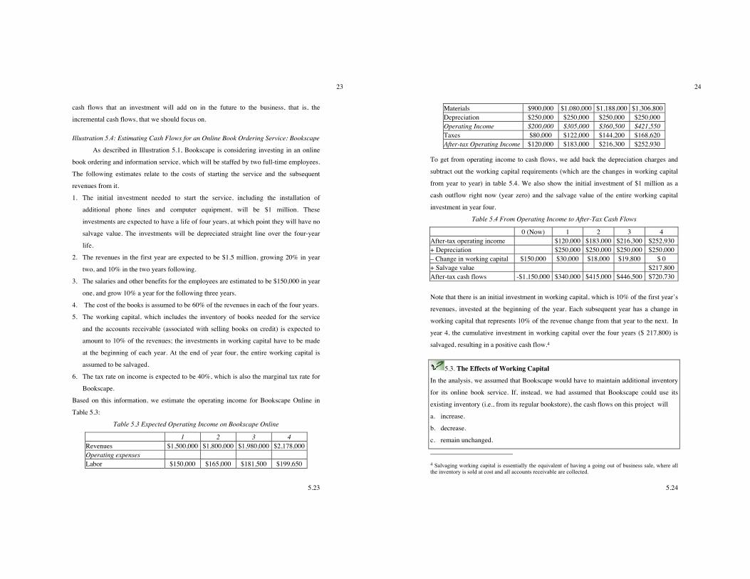
Table 5.3 Expected Operating Income on Bookscape Online

1 2 3 4 Revenues $1,500,000 $1,800,000 $1,980,000 $2,178,000 Operating expenses Labor $150,000 $165,000 $181,500 $199,650

5.24

24

Materials $900,000 $1,080,000 $1,188,000 $1,306,800 Depreciation $250,000 $250,000 $250,000 $250,000 Operating Income $200,000 $305,000 $360,500 $421,550 Taxes $80,000 $122,000 $144,200 $168,620 After-tax Operating Income $120,000 $183,000 $216,300 $252,930

To get from operating income to cash flows, we add back the depreciation charges and

subtract out the working capital requirements (which are the changes in working capital

from year to year) in table 5.4. We also show the initial investment of $1 million as a

cash outflow right now (year zero) and the salvage value of the entire working capital

investment in year four.

Table 5.4 From Operating Income to After-Tax Cash Flows

0 (Now) 1 2 3 4 After-tax operating income $120,000 $183,000 $216,300 $252,930 + Depreciation $250,000 $250,000 $250,000 $250,000 – Change in working capital $150,000 $30,000 $18,000 $19,800 $ 0 + Salvage value $217,800 After-tax cash flows -$1,150,000 $340,000 $415,000 $446,500 $720,730

Note that there is an initial investment in working capital, which is 10% of the first year’s

revenues, invested at the beginning of the year. Each subsequent year has a change in

working capital that represents 10% of the revenue change from that year to the next. In

year 4, the cumulative investment in working capital over the four years ($ 217,800) is

salvaged, resulting in a positive cash flow.4

5.3. The Effects of Working Capital In the analysis, we assumed that Bookscape would have to maintain additional inventory

for its online book service. If, instead, we had assumed that Bookscape could use its

existing inventory (i.e., from its regular bookstore), the cash flows on this project will

a. increase.

b. decrease.

c. remain unchanged.

4 Salvaging working capital is essentially the equivalent of having a going out of business sale, where all the inventory is sold at cost and all accounts receivable are collected.

5.25

25

Explain.

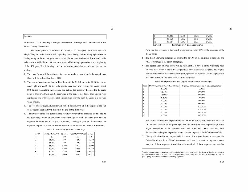
Illustration 5.5: Estimating Earnings, Incremental Earnings and Incremental Cash

Flows: Disney Theme Park

The theme parks to be built near Rio, modeled on Disneyland Paris, will include a

Magic Kingdom to be constructed, beginning immediately, and becoming operational at

the beginning of the second year, and a second theme park modeled on Epcot at Orlando

to be constructed in the second and third year and becoming operational at the beginning

of the fifth year. The following is the set of assumptions that underlie the investment

analysis.

1. The cash flows will be estimated in nominal dollars, even thought he actual cash

flows will be in Brazilian Reals (R$).

2. The cost of constructing Magic Kingdom will be $3 billion, with $2 billion to be

spent right now and $1 billion to be spent a year from now. Disney has already spent

$0.5 billion researching the proposal and getting the necessary licenses for the park;

none of this investment can be recovered if the park is not built. This amount was

capitalized and will be depreciated straight line over the next 10 years to a salvage

value of zero.

3. The cost of constructing Epcot II will be $1.5 billion, with $1 billion spent at the end

of the second year and $0.5 billion at the end of the third year.

4. The revenues at the two parks and the resort properties at the parks are assumed to be

the following, based on projected attendance figures until the tenth year and an

expected inflation rate of 2% (in U.S. dollars). Starting in year ten, the revenues are

expected to grow at the inflation rate. Table 5.5 summarizes the revenue projections:

Table 5.5 Revenue Projections: Rio Disney

Year Magic Kingdom Epcot II Resort Properties Total 1 $0 $0 $0 $0 2 $1,000 $0 $250 $1,250 3 $1,400 $0 $350 $1,750 4 $1,700 $300 $500 $2,500 5 $2,000 $500 $625 $3,125 6 $2,200 $550 $688 $3,438 7 $2,420 $605 $756 $3,781

5.26

26

8 $2,662 $666 $832 $4,159 9 $2,928 $732 $915 $4,559 10 $2,987 $747 $933 $4,667 Beyond Revenues grow 2% a year forever

Note that the revenues at the resort properties are set at 25% of the revenues at the

theme parks.

5. The direct operating expenses are assumed to be 60% of the revenues at the parks and

75% of revenues at the resort properties.

6. The depreciation on fixed assets will be calculated as a percent of the remaining book

value of these assets at the end of the previous year. In addition, the parks will require

capital maintenance investments each year, specified as a percent of the depreciation

that year. Table 5.6 lists both these statistics by year:5

Table 5.6 Depreciation and Capital Maintenance Percentages

Year Depreciation as % of Book Value Capital Maintenance as % of Depreciation 1 0.00% 0.00% 2 12.50% 50.00% 3 11.00% 60.00% 4 9.50% 70.00% 5 8.00% 80.00% 6 8.00% 90.00% 7 8.00% 100.00% 8 8.00% 105.00% 9 8.00% 110.00% 10 8.00% 110.00%

The capital maintenance expenditures are low in the early years, when the parks are

still new but increase as the parks age since old attractions have to go through either

major renovations or be replaced with new attractions. After year ten, both

depreciation and capital expenditures are assumed to grow at the inflation rate (2%).

7. Disney will also allocate corporate G&A costs to this project, based on revenues; the

G&A allocation will be 15% of the revenues each year. It is worth noting that a recent

analysis of these expenses found that only one-third of these expenses are variable

5Capital maintenance expenditures are capital expenditures to replace fixed assets that break down or become obsolete. This is in addition to the regular maintenance expenses that will be necessary to keep the parks going, which are included in operating expenses.

5.27

27

(and a function of total revenue) and that two-thirds are fixed. After year ten, these

expenses are also assumed to grow at the inflation rate of 2%.

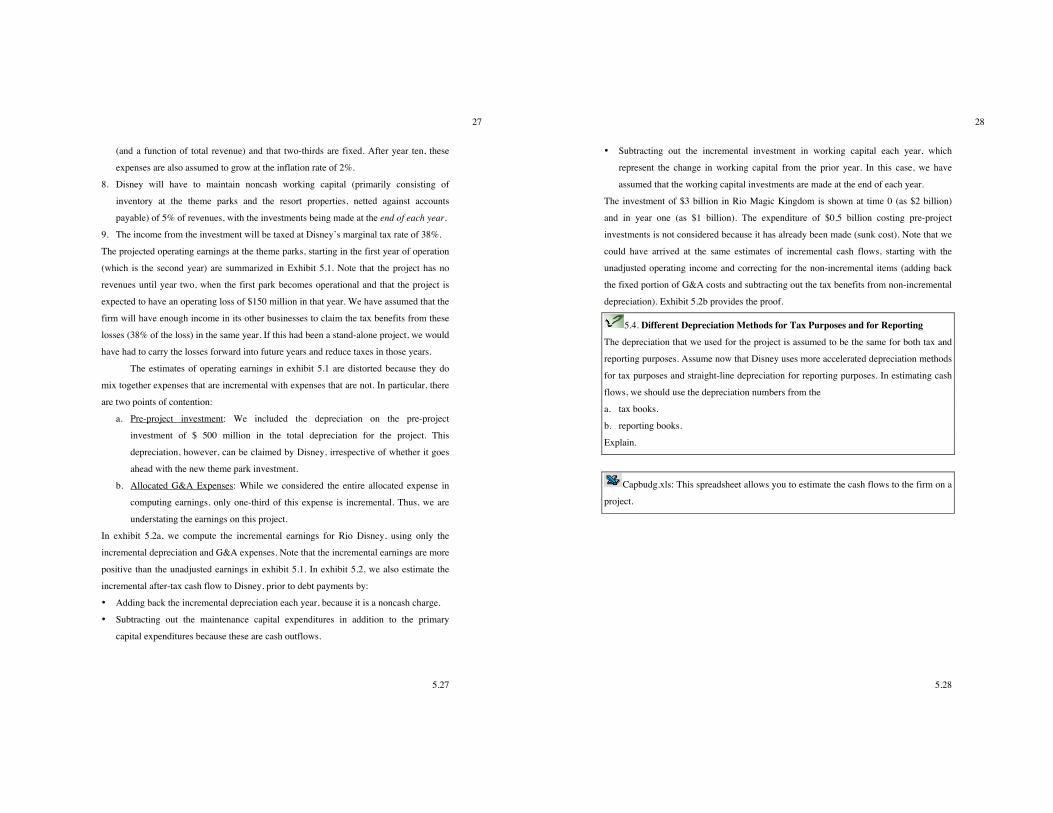
8. Disney will have to maintain noncash working capital (primarily consisting of

inventory at the theme parks and the resort properties, netted against accounts

payable) of 5% of revenues, with the investments being made at the end of each year.

9. The income from the investment will be taxed at Disney’s marginal tax rate of 38%.

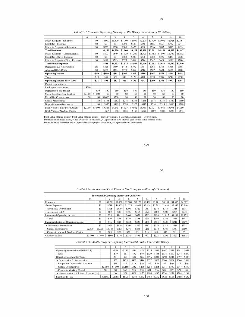
The projected operating earnings at the theme parks, starting in the first year of operation

(which is the second year) are summarized in Exhibit 5.1. Note that the project has no

revenues until year two, when the first park becomes operational and that the project is

expected to have an operating loss of $150 million in that year. We have assumed that the

firm will have enough income in its other businesses to claim the tax benefits from these

losses (38% of the loss) in the same year. If this had been a stand-alone project, we would

have had to carry the losses forward into future years and reduce taxes in those years.

The estimates of operating earnings in exhibit 5.1 are distorted because they do

mix together expenses that are incremental with expenses that are not. In particular, there

are two points of contention:

a. Pre-project investment: We included the depreciation on the pre-project

investment of $ 500 million in the total depreciation for the project. This

depreciation, however, can be claimed by Disney, irrespective of whether it goes

ahead with the new theme park investment.

b. Allocated G&A Expenses: While we considered the entire allocated expense in

computing earnings, only one-third of this expense is incremental. Thus, we are

understating the earnings on this project.

In exhibit 5.2a, we compute the incremental earnings for Rio Disney, using only the

incremental depreciation and G&A expenses. Note that the incremental earnings are more

positive than the unadjusted earnings in exhibit 5.1. In exhibit 5.2, we also estimate the

incremental after-tax cash flow to Disney, prior to debt payments by:

• Adding back the incremental depreciation each year, because it is a noncash charge.

• Subtracting out the maintenance capital expenditures in addition to the primary

capital expenditures because these are cash outflows.

5.28

28

• Subtracting out the incremental investment in working capital each year, which

represent the change in working capital from the prior year. In this case, we have

assumed that the working capital investments are made at the end of each year.

The investment of $3 billion in Rio Magic Kingdom is shown at time 0 (as $2 billion)

and in year one (as $1 billion). The expenditure of $0.5 billion costing pre-project

investments is not considered because it has already been made (sunk cost). Note that we

could have arrived at the same estimates of incremental cash flows, starting with the

unadjusted operating income and correcting for the non-incremental items (adding back

the fixed portion of G&A costs and subtracting out the tax benefits from non-incremental

depreciation). Exhibit 5.2b provides the proof.

5.4. Different Depreciation Methods for Tax Purposes and for Reporting

The depreciation that we used for the project is assumed to be the same for both tax and

reporting purposes. Assume now that Disney uses more accelerated depreciation methods

for tax purposes and straight-line depreciation for reporting purposes. In estimating cash

flows, we should use the depreciation numbers from the

a. tax books.

b. reporting books.

Explain.

Capbudg.xls: This spreadsheet allows you to estimate the cash flows to the firm on a

project.

5.29

29

Exhibit 5.1 Estimated Operating Earnings at Rio Disney (in millions of US dollars)

0 1 2 3 4 5 6 7 8 9 10 Magic Kingdom - Revenues $0 $1,000 $1,400 $1,700 $2,000 $2,200 $2,420 $2,662 $2,928 $2,987 Epcot Rio - Revenues $0 $0 $0 $300 $500 $550 $605 $666 $732 $747 Resort & Properties - Revenues $0 $250 $350 $500 $625 $688 $756 $832 $915 $933 Total Revenues $1,250 $1,750 $2,500 $3,125 $3,438 $3,781 $4,159 $4,575 $4,667 Magic Kingdom – Direct Expenses $0 $600 $840 $1,020 $1,200 $1,320 $1,452 $1,597 $1,757 $1,792 Epcot Rio – Direct Expenses $0 $0 $0 $180 $300 $330 $363 $399 $439 $448 Resort & Property – Direct Expenses $0 $188 $263 $375 $469 $516 $567 $624 $686 $700 Total Direct Expenses $788 $1,103 $1,575 $1,969 $2,166 $2,382 $2,620 $2,882 $2,940 Depreciation & Amortization $50 $425 $469 $444 $372 $367 $364 $364 $366 $368 Allocated G&A Costs $0 $188 $263 $375 $469 $516 $567 $624 $686 $700 Operating Income -$50 -$150 -$84 $106 $315 $389 $467 $551 $641 $658 Taxes -$19 -$57 -$32 $40 $120 $148 $178 $209 $244 $250 Operating Income after Taxes -$31 -$93 -$52 $66 $196 $241 $290 $341 $397 $408 Capital Expenditures Pre-Project investments $500 Depreciation: Pre-Project $50 $50 $50 $50 $50 $50 $50 $50 $50 $50 Magic Kingdom: Construction $2,000 $1,000 $0 $0 $0 $0 $0 $0 $0 $0 $0 Epcot Rio: Construction $0 $0 $1,000 $500 $0 $0 $0 $0 $0 $0 $0 Capital Maintenance $0 $188 $252 $276 $258 $285 $314 $330 $347 $350 Depreciation on fixed assets $0 $375 $419 $394 $322 $317 $314 $314 $316 $318 Book Value of New Fixed Assets $2,000 $3,000 $3,813 $4,145 $4,027 $3,962 $3,931 $3,931 $3,946 $3,978 $4,010 Book Value of Working Capital $63 $88 $125 $156 $172 $189 $208 $229 $233

Book value of fixed assetst= Book value of fixed assetst-1+ New Investmentt + Capital Maintenancet – Depreciationt Depreciation on fixed assetst = Book value of fixed assetst-1* Depreciation as % of prior year’s book value of fixed assets Depreciation & Amortizationt = Depreciation: Pre-project investmentt + Depreciation on fixed assets

5.30

30

Exhibit 5.2a: Incremental Cash Flows at Rio Disney (in millions of US dollars)

Incremental Operating Income and Cash Flow 0 1 2 3 4 5 6 7 8 9 10

Revenues $0 $1,250 $1,750 $2,500 $3,125 $3,438 $3,781 $4,159 $4,575 $4,667 -Direct Expenses $0 $788 $1,103 $1,575 $1,969 $2,166 $2,382 $2,620 $2,882 $2,940 - Incremental Depreciation $0 $375 $419 $394 $322 $317 $314 $314 $316 $318 - Incremental G&A $0 $63 $88 $125 $156 $172 $189 $208 $229 $233 Incremental Operating Income $0 $25 $141 $406 $678 $783 $896 $1,017 $1,148 $1,175 - Taxes $0 $10 $53 $154 $258 $298 $340 $386 $436 $447 Incremental after-tax Operating income $0 $16 $87 $252 $420 $485 $555 $630 $712 $729 + Incremental Depreciation $0 $375 $419 $394 $322 $317 $314 $314 $316 $318 - Capital Expenditures $2,000 $1,000 $1,188 $752 $276 $258 $285 $314 $330 $347 $350 - Change in non-cash Working Capital $0 $63 $25 $38 $31 $16 $17 $19 $21 $5 Cashflow to firm -$2,000 -$1,000 -$860 -$270 $332 $453 $502 $538 $596 $660 $692

Exhibit 5.2b: Another way of computing Incremental Cash Flows at Rio Disney

0 1 2 3 4 5 6 7 8 9 10 Operating income (from Exhibit 5.1) -$50 -$150 -$84 $106 $315 $389 $467 $551 $641 $658 - Taxes -$19 -$57 -$32 $40 $120 $148 $178 $209 $244 $250 Operating Income after Taxes -$31 -$93 -$52 $66 $196 $241 $290 $341 $397 $408 + Depreciation & Amortization $50 $425 $469 $444 $372 $367 $364 $364 $366 $368 - Pre-project Depreciation * tax rate $19 $19 $19 $19 $19 $19 $19 $19 $19 $19 - Capital Expenditures $2,000 $1,000 $1,188 $752 $276 $258 $285 $314 $330 $347 $350 - Change in Working Capital $0 $0 $63 $25 $38 $31 $16 $17 $19 $21 $5 + Non-incremental Allocated Expense (1-t) $0 $78 $109 $155 $194 $213 $234 $258 $284 $289 Cashflow to Firm -$2,000 -$1,000 -$860 -$270 $332 $453 $502 $538 $596 $660 $692

5.31

31

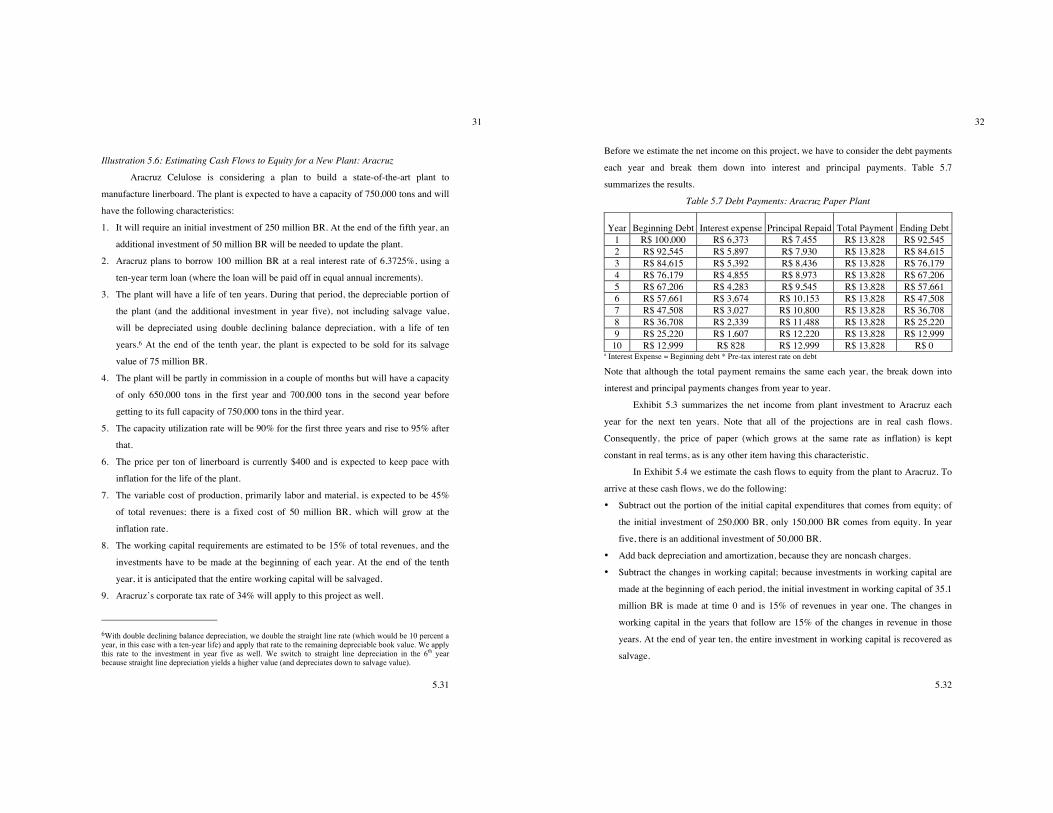
Illustration 5.6: Estimating Cash Flows to Equity for a New Plant: Aracruz

Aracruz Celulose is considering a plan to build a state-of-the-art plant to

manufacture linerboard. The plant is expected to have a capacity of 750,000 tons and will

have the following characteristics:

1. It will require an initial investment of 250 million BR. At the end of the fifth year, an

additional investment of 50 million BR will be needed to update the plant.

2. Aracruz plans to borrow 100 million BR at a real interest rate of 6.3725%, using a

ten-year term loan (where the loan will be paid off in equal annual increments).

3. The plant will have a life of ten years. During that period, the depreciable portion of

the plant (and the additional investment in year five), not including salvage value,

will be depreciated using double declining balance depreciation, with a life of ten

years.6 At the end of the tenth year, the plant is expected to be sold for its salvage

value of 75 million BR.

4. The plant will be partly in commission in a couple of months but will have a capacity

of only 650,000 tons in the first year and 700,000 tons in the second year before

getting to its full capacity of 750,000 tons in the third year.

5. The capacity utilization rate will be 90% for the first three years and rise to 95% after

that.

6. The price per ton of linerboard is currently $400 and is expected to keep pace with

inflation for the life of the plant.

7. The variable cost of production, primarily labor and material, is expected to be 45%

of total revenues; there is a fixed cost of 50 million BR, which will grow at the

inflation rate.

8. The working capital requirements are estimated to be 15% of total revenues, and the

investments have to be made at the beginning of each year. At the end of the tenth

year, it is anticipated that the entire working capital will be salvaged.

9. Aracruz’s corporate tax rate of 34% will apply to this project as well.

6With double declining balance depreciation, we double the straight line rate (which would be 10 percent a year, in this case with a ten-year life) and apply that rate to the remaining depreciable book value. We apply this rate to the investment in year five as well. We switch to straight line depreciation in the 6th year because straight line depreciation yields a higher value (and depreciates down to salvage value).

5.32

32

Before we estimate the net income on this project, we have to consider the debt payments

each year and break them down into interest and principal payments. Table 5.7

summarizes the results.

Table 5.7 Debt Payments: Aracruz Paper Plant

Year Beginning Debt Interest expense Principal Repaid Total Payment Ending Debt 1 R$ 100,000 R$ 6,373 R$ 7,455 R$ 13,828 R$ 92,545 2 R$ 92,545 R$ 5,897 R$ 7,930 R$ 13,828 R$ 84,615 3 R$ 84,615 R$ 5,392 R$ 8,436 R$ 13,828 R$ 76,179 4 R$ 76,179 R$ 4,855 R$ 8,973 R$ 13,828 R$ 67,206 5 R$ 67,206 R$ 4,283 R$ 9,545 R$ 13,828 R$ 57,661 6 R$ 57,661 R$ 3,674 R$ 10,153 R$ 13,828 R$ 47,508 7 R$ 47,508 R$ 3,027 R$ 10,800 R$ 13,828 R$ 36,708 8 R$ 36,708 R$ 2,339 R$ 11,488 R$ 13,828 R$ 25,220 9 R$ 25,220 R$ 1,607 R$ 12,220 R$ 13,828 R$ 12,999

10 R$ 12,999 R$ 828 R$ 12,999 R$ 13,828 R$ 0 a Interest Expense = Beginning debt * Pre-tax interest rate on debt

Note that although the total payment remains the same each year, the break down into

interest and principal payments changes from year to year.

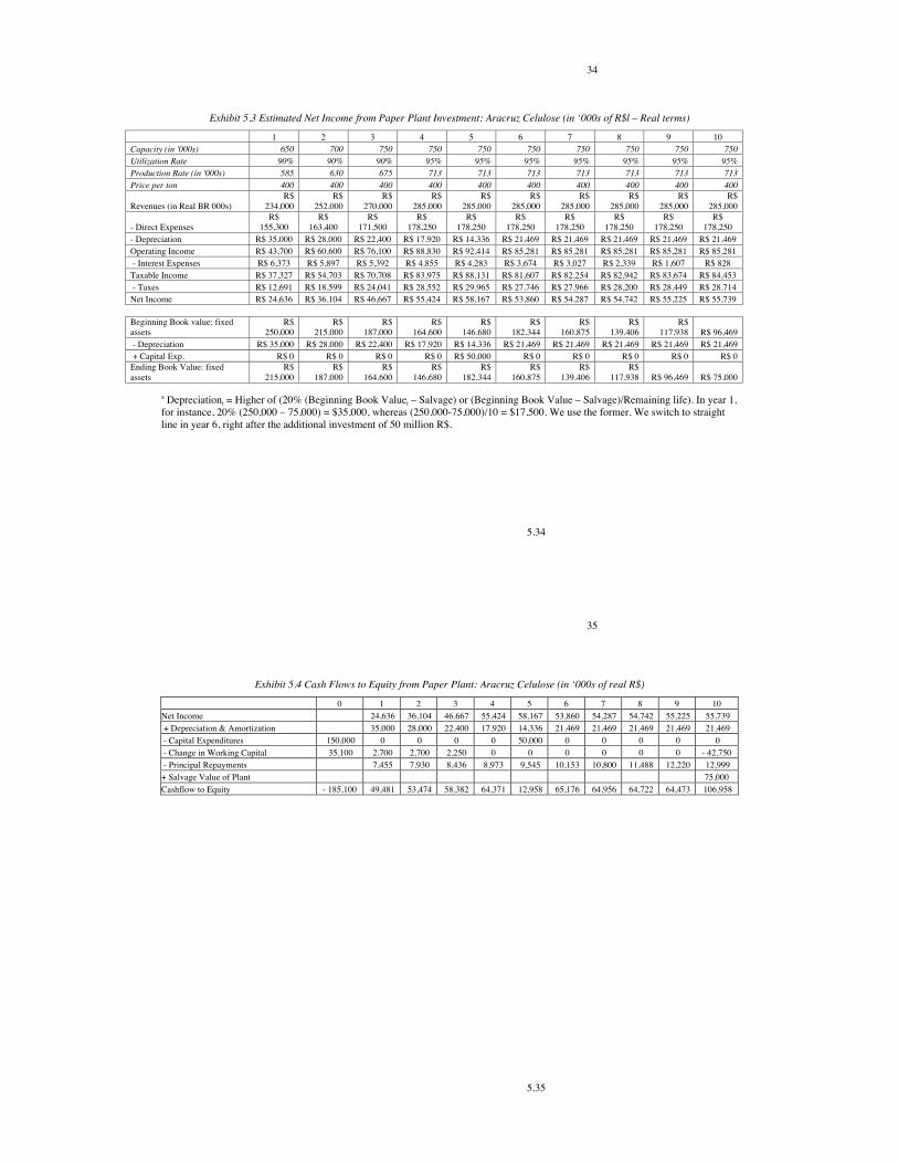
Exhibit 5.3 summarizes the net income from plant investment to Aracruz each

year for the next ten years. Note that all of the projections are in real cash flows.

Consequently, the price of paper (which grows at the same rate as inflation) is kept

constant in real terms, as is any other item having this characteristic.

In Exhibit 5.4 we estimate the cash flows to equity from the plant to Aracruz. To

arrive at these cash flows, we do the following:

• Subtract out the portion of the initial capital expenditures that comes from equity; of

the initial investment of 250,000 BR, only 150,000 BR comes from equity. In year

five, there is an additional investment of 50,000 BR.

• Add back depreciation and amortization, because they are noncash charges.

• Subtract the changes in working capital; because investments in working capital are

made at the beginning of each period, the initial investment in working capital of 35.1

million BR is made at time 0 and is 15% of revenues in year one. The changes in

working capital in the years that follow are 15% of the changes in revenue in those

years. At the end of year ten, the entire investment in working capital is recovered as

salvage.

5.33

33

• Subtract the principal payments that are made to the bank in each period, because

these are cash outflows to the nonequity claimholders in the firm.

• Add the salvage value of the plant in year ten to the total cash flows, because this is a

cash inflow to equity investors.

The cash flows to equity measure the cash flows that equity investors at Aracruz can

expect to receive from investing in the plant.

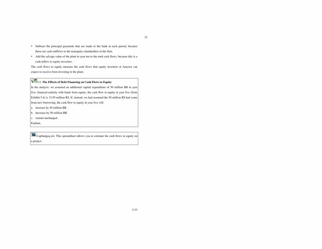
5.5. The Effects of Debt Financing on Cash Flows to Equity

In the analysis, we assumed an additional capital expenditure of 50 million BR in year

five, financed entirely with funds from equity; the cash flow to equity in year five (from

Exhibit 5.4) is 12.95 million R$. If, instead, we had assumed the 50 million R$ had come

from new borrowing, the cash flow to equity in year five will

a. increase by 50 million BR.

b. decrease by 50 million BR.

c. remain unchanged.

Explain.

Capbudgeq.xls: This spreadsheet allows you to estimate the cash flows to equity on

a project.

5.34

34

Exhibit 5.3 Estimated Net Income from Paper Plant Investment: Aracruz Celulose (in ‘000s of R$l – Real terms)

1 2 3 4 5 6 7 8 9 10 Capacity (in '000s) 650 700 750 750 750 750 750 750 750 750 Utilization Rate 90% 90% 90% 95% 95% 95% 95% 95% 95% 95% Production Rate (in '000s) 585 630 675 713 713 713 713 713 713 713 Price per ton 400 400 400 400 400 400 400 400 400 400

Revenues (in Real BR 000s) R$

234,000 R$

252,000 R$

270,000 R$

285,000 R$

285,000 R$

285,000 R$

285,000 R$

285,000 R$

285,000 R$

285,000

- Direct Expenses R$

155,300 R$

163,400 R$

171,500 R$

178,250 R$

178,250 R$

178,250 R$

178,250 R$

178,250 R$

178,250 R$

178,250 - Depreciation R$ 35,000 R$ 28,000 R$ 22,400 R$ 17,920 R$ 14,336 R$ 21,469 R$ 21,469 R$ 21,469 R$ 21,469 R$ 21,469 Operating Income R$ 43,700 R$ 60,600 R$ 76,100 R$ 88,830 R$ 92,414 R$ 85,281 R$ 85,281 R$ 85,281 R$ 85,281 R$ 85,281 - Interest Expenses R$ 6,373 R$ 5,897 R$ 5,392 R$ 4,855 R$ 4,283 R$ 3,674 R$ 3,027 R$ 2,339 R$ 1,607 R$ 828 Taxable Income R$ 37,327 R$ 54,703 R$ 70,708 R$ 83,975 R$ 88,131 R$ 81,607 R$ 82,254 R$ 82,942 R$ 83,674 R$ 84,453 - Taxes R$ 12,691 R$ 18,599 R$ 24,041 R$ 28,552 R$ 29,965 R$ 27,746 R$ 27,966 R$ 28,200 R$ 28,449 R$ 28,714 Net Income R$ 24,636 R$ 36,104 R$ 46,667 R$ 55,424 R$ 58,167 R$ 53,860 R$ 54,287 R$ 54,742 R$ 55,225 R$ 55,739 Beginning Book value: fixed assets

R$ 250,000

R$ 215,000

R$ 187,000

R$ 164,600

R$ 146,680

R$ 182,344

R$ 160,875

R$ 139,406

R$ 117,938 R$ 96,469

- Depreciation R$ 35,000 R$ 28,000 R$ 22,400 R$ 17,920 R$ 14,336 R$ 21,469 R$ 21,469 R$ 21,469 R$ 21,469 R$ 21,469 + Capital Exp. R$ 0 R$ 0 R$ 0 R$ 0 R$ 50,000 R$ 0 R$ 0 R$ 0 R$ 0 R$ 0 Ending Book Value: fixed assets

R$ 215,000

R$ 187,000

R$ 164,600

R$ 146,680

R$ 182,344

R$ 160,875

R$ 139,406

R$ 117,938 R$ 96,469 R$ 75,000

a Depreciationt = Higher of (20% (Beginning Book Valuet – Salvage) or (Beginning Book Value – Salvage)/Remaining life). In year 1, for instance, 20% (250,000 – 75,000) = $35,000, whereas (250,000-75,000)/10 = $17,500. We use the former. We switch to straight line in year 6, right after the additional investment of 50 million R$.

5.35

35

Exhibit 5.4 Cash Flows to Equity from Paper Plant: Aracruz Celulose (in ‘000s of real R$)

0 1 2 3 4 5 6 7 8 9 10 Net Income 24,636 36,104 46,667 55,424 58,167 53,860 54,287 54,742 55,225 55,739 + Depreciation & Amortization 35,000 28,000 22,400 17,920 14,336 21,469 21,469 21,469 21,469 21,469 - Capital Expenditures 150,000 0 0 0 0 50,000 0 0 0 0 0 - Change in Working Capital 35,100 2,700 2,700 2,250 0 0 0 0 0 0 - 42,750 - Principal Repayments 7,455 7,930 8,436 8,973 9,545 10,153 10,800 11,488 12,220 12,999 + Salvage Value of Plant 75,000 Cashflow to Equity - 185,100 49,481 53,474 58,382 64,371 12,958 65,176 64,956 64,722 64,473 106,958

5.36

36

Illustration 5.7: Estimating Cash flows from an acquisition: Sensient Technologies

To evaluate how much Tata Chemicals should pay for Sensient Technologies, we

estimated the cash flows from the entire firm. As with the Disney analysis, we will

estimate pre-debt cash flows, i.e., cash flow to the firm, using the same steps. We will

begin with the after-tax operating income, add back depreciation and other non-cash

charges and subtract out changes in non-cash working capital. There are two key

differences between valuing a firm and valuing a project. The first is that a publicly

traded firm, at least in theory, can have a perpetual life. Most projects have finite lives,

though we will argue that projects such as theme parks may have lives so long that we

could treat them as having infinite lives. The second is that a firm can be considered a

portfolio of projects, current and future. As a consequence, to value a firm, we have to

make judgments about the quantity and quality of future projects.

For Sensient Technologies, we started with the 2008 financial statements and

obtained the following inputs for cash flow in 2008:

a. Operating Income: The firm reported operating income of $162 million on

revenues of $1.23 billion for the year. The firm paid 37% of its income as taxes in

2008, and we will use this as both the effective and marginal tax rate.

b. Capital Expenditures and depreciation: Depreciation in 2008 amounted to $44

million, whereas capital expenditures for the year was $54 million. Non-cash

working capital increased by approximately $16 million during the year.

The cash flow to the firm for Sensient Technologies in 2008 can be estimated as follows:

Cash Flow to the firm = After-tax Operating Income + Depreciation – Capital

Expenditures – Change in Non-cash Working Capital = 162 (1-.37) + 44 – 54 –

16 = $76.06 million

We will assume that the firm is mature and that all of the inputs to this computation –

earnings, capital expenditures, depreciation and working capital – will grow 2% a year in

perpetuity.7

7 For the moment, this assumption seems to be an arbitrary one. Clearly, we need to give more thought to not only what a reasonable growth rate for a firm is but what may cause that growth rate to change. We will return to this issue in much more depth in chapter 12 and use this simplified example for this chapter.

5.37

37

In Practice: Estimating Expected Revenues and Cash Flows

How do we estimate a project’s expected revenues and expenses? The key word

in this question is estimate. No one, no matter what his or her skill at forecasting and

degree of preparation, can forecast with certainty how a risky project will do. There are

generally three ways in which we can make these forecasts:

a. Experience and History: The process of estimating project revenues and expenses is

simplest for firms that consider the same kind of projects repeatedly. These firms can

use their experience from similar projects that are already in operation to estimate

expected values for new projects. Disney, for instance, can use its experiences with its

existing theme parks in making its estimates for Rio Disney.

b. Market Testing: If the project being assessed is different from the firm’s existing

business, we may need a preliminary assessment of the market before actually

investing in the project. In a market survey, potential customers are asked about the

product or service being considered to gauge the interest they would have in

acquiring it. The results usually are qualitative and indicate whether the interest is

strong or weak, allowing the firm to decide whether to use optimistic forecasts for

revenues (if the interest is strong) or pessimistic forecasts (if the interest is weak).

Companies that need more information will often test market the concept on smaller

markets, before introducing it on a larger scale. Test marketing not only allows firms

to test out the product or service directly but also yields far more detailed information

about the potential size of the market.

c. Scenario Analysis: There are cases in which a firm is considering introducing a

product to a market it knows well, but there is considerable uncertainty introduced by

external factors that the firm cannot control. In such cases, a firm may decide to

consider different scenarios, and the revenues and expenses on the project under each

scenario. We will return to this approach later in this chapter.

We have laid out three ways of estimating revenues and expenses for projects, but none

of these approaches yields perfect estimates. Although some project risk may come from

estimation error, a large portion of risk comes from real uncertainty about the future.

Improving estimation techniques, using more market testing, and performing scenario

5.38

38

analysis may reduce estimation error but cannot eliminate real uncertainty. This is why

we incorporate a risk premium into the discount rate.

C. Time-Weighted versus Nominal Cash Flows Very few projects with long lifetimes generate earnings or cash flows evenly over

their lives. In sectors with huge investments in infrastructure, such as

telecommunications, the earnings and cash flows might be negative for an extended

period (say, ten to twenty years) before they turn positive. In other sectors, the cashflows

peak early and then gradually decrease over time. Whatever the reason for the

unevenness of cash flows, a basic question that has to be addressed when measuring

returns is whether they should reflect the timing of the earnings or cash flows. We will

argue that they should, with earlier earnings and cash flows being weighted more when

computing returns than earnings and cash flows later in a project life.

Why Cash Flows across Time Are Not Comparable

There are three reasons why cash flows across time are not comparable, and a cash

flow in the future is worth less than a similar cash flow today:

1. Individuals prefer present consumption to future consumption. People would have to

be offered more in the future to give up present consumption—this is called the real

rate of return. The greater the real rate of return, the greater the difference in value

between a cash flow today and an equal cash flow in the future.

2. When there is monetary inflation, the value of currency decreases over time. The

greater the inflation, the greater the difference in value between a cash flow today and

an equal cash flow in the future.

3. Any uncertainty (risk) associated with the cash flow in the future reduces the value of

the cash flow. The greater the uncertainty associated with the cash flow, the greater the

difference between receiving the cash flow today and receiving an equal amount in the

future.

The process by which future cash flows are adjusted to reflect these factors is called

discounting, and the magnitude of these factors is reflected in the discount rate. Thus the

present value of a cash flow (CFt) at a point in time t in the future, when the discount rate

is r, can be written as follows:

5.39

39

Present Value of Cash Flow = CFt 1

(1+ r)t!

" # $

%

Note that the second term in the brackets, (1/[1 + r]t), is called the discount factor and

effectively weights the cash flow by when it occurs. The differences in weights across

time will depend entirely on the level of the discount rate. Consequently, when discount

rates are high, which could be due to high real rates, high inflation, and/or high

uncertainty, returns that occur further in the future will be weighted less. Appendix 3

includes a more complete discussion of the mechanics of present value.

The Case for Time-Weighted Returns

If we accept the arguments that cash flows measure returns more accurately than

earnings and that the incremental cash flows more precisely estimate returns than total

cash flows, we should logically follow up by using discounted cash flows (i.e., time-

weighted returns) rather than nominal cash flows for two reasons.

1. Nominal cash flows at different points in time are not comparable and cannot be

aggregated to arrive at returns. Discounted cash flows, on the other hand, convert all

cash flows on a project to today’s terms and allow us to compute returns more

consistently.

2. If the objective in investment analysis is to maximize the value of the business taking

the investments, we should be weighting cash flows that occur early more than cash

flow that occur later, because investors in the business will also do so.

5.6. Time Horizons and Time Weighting

Calculating present values for cash flows leads to a greater weighting for cash flows that

occur sooner and a lower weighting for cash flows that occur later. Does it necessarily

follow that using present value (as opposed to nominal value) makes managers more

likely to take short-term projects over long-term projects?

Yes

No

Why or why not?

5.40

40

Managerial Optimism and Cash Flow Estimation

There is substantial evidence that managers tend to be too optimistic when

assessing outcomes from an investment, and systematically overestimate the cash flows

on investments. From capital budgeting projects, where expected revenues are higher

than expected and costs are lower than expected, to acquisitions, where the projected cash

flows on target companies are much higher than actual cash flows, there is an “optimism

bias” that leads firms to take many investments that should not be accepted.8

The literature on managerial optimism also has two key sub-findings. The first is

that people are more optimistic about outcomes that they believe that they can control.

Thus, managers often over estimate their capacity to deliver market share and profit

margins, in the face of competition. The second is that optimism tends to increase with

commitment; the more committed a manager is to an investment, the more he or she is

likely to over estimate the cash flows from that investment. These findings suggests two

possible solutions to the optimism bias. The first is to take away the project analysis

duties away from the project advocates. In other words, managers should not be given the

task of generating the expected cash flows from expansion opportunities that they have

initiated. In the same vein, investment bankers touting potential target companies for

acquisitions should not be generating the expected cash flows for the valuations of these

companies. The second is a requirement that all investments, no matter what their

pedigree and who advocates them, be put through stress tests, where key assumptions are

questioned, changed and analyzed.

To those who believe that hiring more experienced or intelligent managers will

solve this problem, there is substantial evidence that the optimism bias becomes worse as

managers become more intelligent and with greater experience. In fact, it is to counter

this bias that firms often set hurdle rates well above the cost of capital or require net

present values to be much greater than zero for a project to pass muster.

8 Heaton, J.B., 2002, “Managerial optimism and corporate finance.” Financial Management 33-45.

5.41

41

Investment Decision Rules Having estimated the accounting earnings, cash flows, and time-weighted cash

flows on an investment, we are still faced with the crucial decision of whether we should

take the investment. In this section, we will consider a series of investment decision rules

and put them to the test.

What Is an Investment Decision Rule? When faced with new investments and projects, firms have to decide whether to

invest in them or not. We have been leading up to this decision over the last few chapters,

but investment decision rules allow us to formalize the process and specify what

conditions need to be met for a project to be acceptable. Although we will be looking at a

variety of investment decision rules in this section, it is worth keeping in mind what

characteristics we would like a good investment decision rule to have.

• First, a good investment decision rule has to maintain a fair balance between allowing

a manager analyzing a project to bring in his or her subjective assessments into the

decision and ensuring that different projects are judged consistently. Thus, an

investment decision rule that is too mechanical (by not allowing for subjective inputs)

or too malleable (where managers can bend the rule to match their biases) is not a

good rule.

• Second, a good investment decision rule will allow the firm to further the stated

objective in corporate finance, which is to maximize the value of the firm. Projects

that are acceptable using the decision rule should increase the value of the firm

accepting them, whereas projects that do not meet the requirements would destroy

value if the firm invested in them.

• Third, a good investment decision rule should work across a variety of investments.

Investments can be revenue-generating investments (such as Home Depot opening a

new store) or they can be cost-saving investments (as would be the case if Boeing

adopted a new system to manage inventory). Some projects have large up-front costs

(as is the case with the Boeing Super Jumbo aircraft), whereas other projects may

have costs spread out across time. A good investment rule will provide an answer on

all of these different kinds of investments.

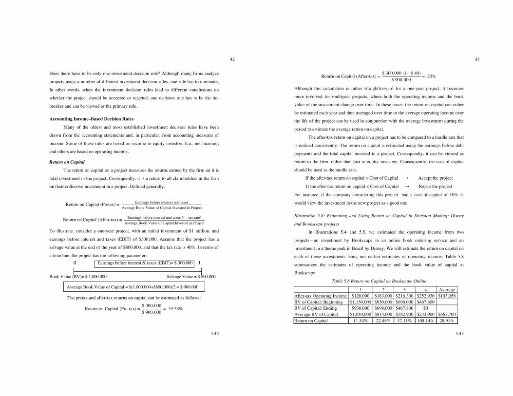
5.42

42

Does there have to be only one investment decision rule? Although many firms analyze

projects using a number of different investment decision rules, one rule has to dominate.

In other words, when the investment decision rules lead to different conclusions on

whether the project should be accepted or rejected, one decision rule has to be the tie-

breaker and can be viewed as the primary rule.

Accounting Income–Based Decision Rules

Many of the oldest and most established investment decision rules have been

drawn from the accounting statements and, in particular, from accounting measures of

income. Some of these rules are based on income to equity investors (i.e., net income),

and others are based on operating income.

Return on Capital

The return on capital on a project measures the returns earned by the firm on it is

total investment in the project. Consequently, it is a return to all claimholders in the firm

on their collective investment in a project. Defined generally,

Return on Capital (Pretax) =

!

Earnings before interest and taxesAverage Book Value of Capital Invested in Project

Return on Capital (After-tax) =

!

Earnings before interest and taxes (1- tax rate)Average Book Value of Capital Invested in Project

To illustrate, consider a one-year project, with an initial investment of $1 million, and

earnings before interest and taxes (EBIT) of $300,000. Assume that the project has a

salvage value at the end of the year of $800,000, and that the tax rate is 40%. In terms of

a time line, the project has the following parameters:

Book Value (BV)= $ 1,000,000 Salvage Value = $ 800,000

Earnings before interest & taxes (EBIT)= $ 300,000

Average Book Value of Capital = $(1,000,000+$800,000)/2 = $ 900,000

0 1

The pretax and after-tax returns on capital can be estimated as follows:

Return on Capital (Pre-tax) = $ 300,000$ 900,000

= 33.33%

5.43

43

Return on Capital (After-tax) = $ 300,000 (1- 0.40)$ 900,000

= 20%

Although this calculation is rather straightforward for a one-year project, it becomes

more involved for multiyear projects, where both the operating income and the book

value of the investment change over time. In these cases, the return on capital can either

be estimated each year and then averaged over time or the average operating income over

the life of the project can be used in conjunction with the average investment during the

period to estimate the average return on capital.

The after-tax return on capital on a project has to be compared to a hurdle rate that

is defined consistently. The return on capital is estimated using the earnings before debt

payments and the total capital invested in a project. Consequently, it can be viewed as

return to the firm, rather than just to equity investors. Consequently, the cost of capital

should be used as the hurdle rate.

If the after-tax return on capital > Cost of Capital ! Accept the project

If the after-tax return on capital < Cost of Capital ! Reject the project

For instance, if the company considering this project had a cost of capital of 10%, it

would view the investment in the new project as a good one.

Illustration 5.8: Estimating and Using Return on Capital in Decision Making: Disney

and Bookscape projects

In Illustrations 5.4 and 5.5, we estimated the operating income from two

projects—an investment by Bookscape in an online book ordering service and an

investment in a theme park in Brazil by Disney. We will estimate the return on capital on

each of these investments using our earlier estimates of operating income. Table 5.8

summarizes the estimates of operating income and the book value of capital at

Bookscape.

Table 5.8 Return on Capital on Bookscape Online

1 2 3 4 Average After-tax Operating Income $120,000 $183,000 $216,300 $252,930 $193,058 BV of Capital: Beginning $1,150,000 $930,000 $698,000 $467,800 BV of Capital: Ending $930,000 $698,000 $467,800 $0 Average BV of Capital $1,040,000 $814,000 $582,900 $233,900 $667,700 Return on Capital 11.54% 22.48% 37.11% 108.14% 28.91%

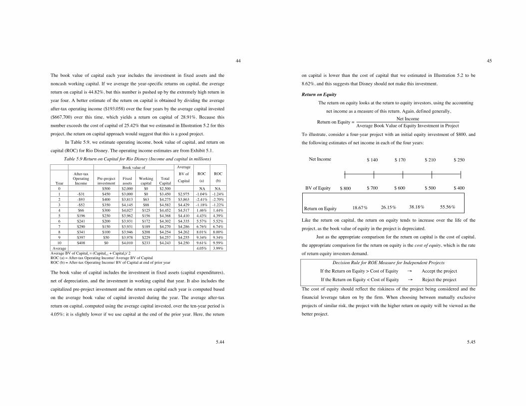
5.44

44

The book value of capital each year includes the investment in fixed assets and the

noncash working capital. If we average the year-specific returns on capital, the average

return on capital is 44.82%, but this number is pushed up by the extremely high return in

year four. A better estimate of the return on capital is obtained by dividing the average

after-tax operating income ($193,058) over the four years by the average capital invested

($667,700) over this time, which yields a return on capital of 28.91%. Because this

number exceeds the cost of capital of 25.42% that we estimated in Illustration 5.2 for this

project, the return on capital approach would suggest that this is a good project.

In Table 5.9, we estimate operating income, book value of capital, and return on

capital (ROC) for Rio Disney. The operating income estimates are from Exhibit 5.1.

Table 5.9 Return on Capital for Rio Disney (Income and capital in millions)

Book value of

Year

After-tax Operating

Income Pre-project investment

Fixed assets

Working capital

Total Capital

Average

BV of

Capital

ROC

(a)

ROC

(b)

0 $500 $2,000 $0 $2,500 NA NA 1 -$31 $450 $3,000 $0 $3,450 $2,975 -1.04% -1.24% 2 -$93 $400 $3,813 $63 $4,275 $3,863 -2.41% -2.70% 3 -$52 $350 $4,145 $88 $4,582 $4,429 -1.18% -1.22% 4 $66 $300 $4,027 $125 $4,452 $4,517 1.46% 1.44% 5 $196 $250 $3,962 $156 $4,368 $4,410 4.43% 4.39% 6 $241 $200 $3,931 $172 $4,302 $4,335 5.57% 5.52% 7 $290 $150 $3,931 $189 $4,270 $4,286 6.76% 6.74% 8 $341 $100 $3,946 $208 $4,254 $4,262 8.01% 8.00% 9 $397 $50 $3,978 $229 $4,257 $4,255 9.34% 9.34%

10 $408 $0 $4,010 $233 $4,243 $4,250 9.61% 9.59% Average 4.05% 3.99%

Average BV of Capitalt = (Capitalt-1 + Capitalt)/ 2 ROC (a) = After-tax Operating Income/ Average BV of Capital ROC (b) = After-tax Operating Income/ BV of Capital at end of prior year

The book value of capital includes the investment in fixed assets (capital expenditures),

net of depreciation, and the investment in working capital that year. It also includes the

capitalized pre-project investment and the return on capital each year is computed based

on the average book value of capital invested during the year. The average after-tax

return on capital, computed using the average capital invested, over the ten-year period is

4.05%; it is slightly lower if we use capital at the end of the prior year. Here, the return

5.45

45

on capital is lower than the cost of capital that we estimated in Illustration 5.2 to be

8.62%, and this suggests that Disney should not make this investment.

Return on Equity

The return on equity looks at the return to equity investors, using the accounting

net income as a measure of this return. Again, defined generally,

Return on Equity = Net IncomeAverage Book Value of Equity Investment in Project

To illustrate, consider a four-year project with an initial equity investment of $800, and

the following estimates of net income in each of the four years:

Net Income

BV of Equity

$ 140 $ 170 $ 210 $ 250

$ 800 $ 700 $ 600 $ 500 $ 400

Return on Equity 18.67% 26.15% 38.18% 55.56%

Like the return on capital, the return on equity tends to increase over the life of the

project, as the book value of equity in the project is depreciated.

Just as the appropriate comparison for the return on capital is the cost of capital,

the appropriate comparison for the return on equity is the cost of equity, which is the rate

of return equity investors demand.

Decision Rule for ROE Measure for Independent Projects

If the Return on Equity > Cost of Equity ! Accept the project

If the Return on Equity < Cost of Equity ! Reject the project

The cost of equity should reflect the riskiness of the project being considered and the

financial leverage taken on by the firm. When choosing between mutually exclusive

projects of similar risk, the project with the higher return on equity will be viewed as the

better project.

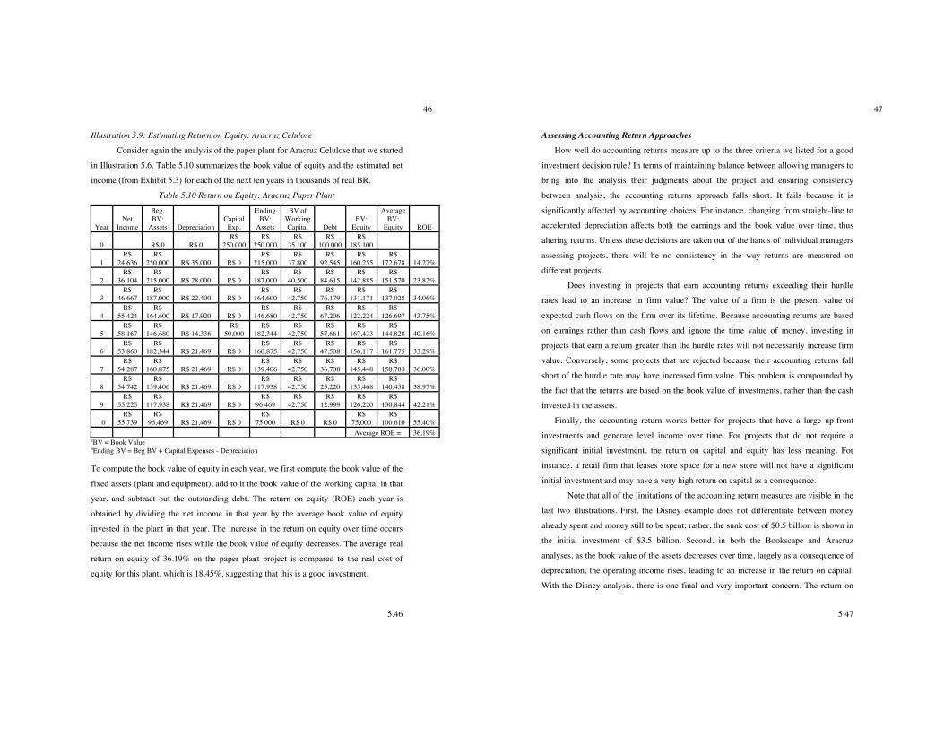
5.46

46

Illustration 5.9: Estimating Return on Equity: Aracruz Celulose

Consider again the analysis of the paper plant for Aracruz Celulose that we started

in Illustration 5.6. Table 5.10 summarizes the book value of equity and the estimated net

income (from Exhibit 5.3) for each of the next ten years in thousands of real BR.

Table 5.10 Return on Equity: Aracruz Paper Plant

Year Net

Income

Beg. BV:

Assets Depreciation Capital

Exp.

Ending BV:

Assets

BV of Working Capital Debt

BV: Equity

Average BV:

Equity ROE

0 R$ 0 R$ 0 R$

250,000 R$

250,000 R$

35,100 R$

100,000 R$

185,100

1 R$

24,636 R$

250,000 R$ 35,000 R$ 0 R$

215,000 R$

37,800 R$

92,545 R$

160,255 R$

172,678 14.27%

2 R$

36,104 R$

215,000 R$ 28,000 R$ 0 R$

187,000 R$

40,500 R$

84,615 R$

142,885 R$

151,570 23.82%

3 R$

46,667 R$

187,000 R$ 22,400 R$ 0 R$

164,600 R$

42,750 R$

76,179 R$

131,171 R$

137,028 34.06%

4 R$

55,424 R$

164,600 R$ 17,920 R$ 0 R$

146,680 R$

42,750 R$

67,206 R$

122,224 R$

126,697 43.75%

5 R$

58,167 R$

146,680 R$ 14,336 R$

50,000 R$

182,344 R$

42,750 R$

57,661 R$

167,433 R$

144,828 40.16%

6 R$

53,860 R$

182,344 R$ 21,469 R$ 0 R$

160,875 R$

42,750 R$

47,508 R$

156,117 R$

161,775 33.29%

7 R$

54,287 R$

160,875 R$ 21,469 R$ 0 R$

139,406 R$

42,750 R$

36,708 R$

145,448 R$

150,783 36.00%

8 R$

54,742 R$

139,406 R$ 21,469 R$ 0 R$

117,938 R$

42,750 R$

25,220 R$

135,468 R$

140,458 38.97%

9 R$

55,225 R$

117,938 R$ 21,469 R$ 0 R$

96,469 R$

42,750 R$

12,999 R$

126,220 R$

130,844 42.21%

10 R$

55,739 R$

96,469 R$ 21,469 R$ 0 R$

75,000 R$ 0 R$ 0 R$

75,000 R$

100,610 55.40% Average ROE = 36.19%

aBV = Book Value bEnding BV = Beg BV + Capital Expenses - Depreciation

To compute the book value of equity in each year, we first compute the book value of the

fixed assets (plant and equipment), add to it the book value of the working capital in that

year, and subtract out the outstanding debt. The return on equity (ROE) each year is

obtained by dividing the net income in that year by the average book value of equity

invested in the plant in that year. The increase in the return on equity over time occurs

because the net income rises while the book value of equity decreases. The average real

return on equity of 36.19% on the paper plant project is compared to the real cost of

equity for this plant, which is 18.45%, suggesting that this is a good investment.

5.47

47

Assessing Accounting Return Approaches

How well do accounting returns measure up to the three criteria we listed for a good

investment decision rule? In terms of maintaining balance between allowing managers to

bring into the analysis their judgments about the project and ensuring consistency

between analysis, the accounting returns approach falls short. It fails because it is

significantly affected by accounting choices. For instance, changing from straight-line to

accelerated depreciation affects both the earnings and the book value over time, thus

altering returns. Unless these decisions are taken out of the hands of individual managers

assessing projects, there will be no consistency in the way returns are measured on

different projects.

Does investing in projects that earn accounting returns exceeding their hurdle

rates lead to an increase in firm value? The value of a firm is the present value of

expected cash flows on the firm over its lifetime. Because accounting returns are based

on earnings rather than cash flows and ignore the time value of money, investing in

projects that earn a return greater than the hurdle rates will not necessarily increase firm

value. Conversely, some projects that are rejected because their accounting returns fall

short of the hurdle rate may have increased firm value. This problem is compounded by

the fact that the returns are based on the book value of investments, rather than the cash

invested in the assets.

Finally, the accounting return works better for projects that have a large up-front

investments and generate level income over time. For projects that do not require a

significant initial investment, the return on capital and equity has less meaning. For

instance, a retail firm that leases store space for a new store will not have a significant

initial investment and may have a very high return on capital as a consequence.

Note that all of the limitations of the accounting return measures are visible in the

last two illustrations. First, the Disney example does not differentiate between money

already spent and money still to be spent; rather, the sunk cost of $0.5 billion is shown in

the initial investment of $3.5 billion. Second, in both the Bookscape and Aracruz

analyses, as the book value of the assets decreases over time, largely as a consequence of

depreciation, the operating income rises, leading to an increase in the return on capital.

With the Disney analysis, there is one final and very important concern. The return on

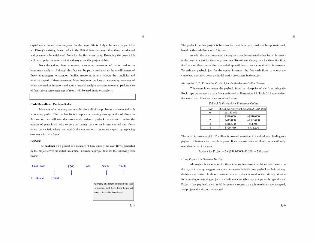
5.48

48

capital was estimated over ten years, but the project life is likely to be much longer. After

all, Disney’s existing theme parks in the United States are more than three decades old

and generate substantial cash flows for the firm even today. Extending the project life

will push up the return on capital and may make this project viable.

Notwithstanding these concerns, accounting measures of return endure in

investment analysis. Although this fact can be partly attributed to the unwillingness of

financial managers to abandon familiar measures, it also reflects the simplicity and

intuitive appeal of these measures. More important, as long as accounting measures of

return are used by investors and equity research analysts to assess to overall performance

of firms, these same measures of return will be used in project analysis.

Cash Flow–Based Decision Rules

Measures of accounting return suffer from all of the problems that we noted with

accounting profits. The simplest fix is to replace accounting earnings with cash flows. In

this section, we will consider two simple variants: payback, where we examine the

number of years it will take to get your money back on an investment and cash flows

return on capital, where we modify the conventional return on capital by replacing

earnings with cash flows.

Payback

The payback on a project is a measure of how quickly the cash flows generated

by the project cover the initial investment. Consider a project that has the following cash

flows:

Payback: The length of time it will take

for nominal cash flows from the project

to cover the initial investment.

5.49

49

The payback on this project is between two and three years and can be approximated,

based on the cash flows to be 2.6 years.

As with the other measures, the payback can be estimated either for all investors

in the project or just for the equity investors. To estimate the payback for the entire firm,

the free cash flows to the firm are added up until they cover the total initial investment.

To estimate payback just for the equity investors, the free cash flows to equity are

cumulated until they cover the initial equity investment in the project.

Illustration 5.10: Estimating Payback for the Bookscape Online Service

This example estimates the payback from the viewpoint of the firm, using the

Bookscape online service cash flows estimated in Illustration 5.4. Table 5.11 summarizes

the annual cash flows and their cumulated value.

Table 5.11 Payback for Bookscape Online

Year Cash flow in year Cumulated Cash flow 0 –$1,150,000 1 $340,000 –$810,000 2 $415,000 –$395,000 3 $446,500 $51,500 4 $720,730 $772,230

The initial investment of $1.15 million is covered sometime in the third year, leading to a

payback of between two and three years. If we assume that cash flows occur uniformly

over the course of the year:

Payback for Project = 2 + ($395,000/$446,500) = 2.88 years

Using Payback in Decision Making

Although it is uncommon for firms to make investment decisions based solely on

the payback, surveys suggest that some businesses do in fact use payback as their primary

decision mechanism. In those situations where payback is used as the primary criterion

for accepting or rejecting projects, a maximum acceptable payback period is typically set.

Projects that pay back their initial investment sooner than this maximum are accepted,

and projects that do not are rejected.

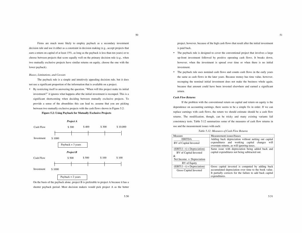
5.50

50

Firms are much more likely to employ payback as a secondary investment

decision rule and use it either as a constraint in decision making (e.g., accept projects that

earn a return on capital of at least 15%, as long as the payback is less than ten years) or to

choose between projects that score equally well on the primary decision rule (e.g., when

two mutually exclusive projects have similar returns on equity, choose the one with the

lower payback).

Biases, Limitations, and Caveats

The payback rule is a simple and intuitively appealing decision rule, but it does

not use a significant proportion of the information that is available on a project.

• By restricting itself to answering the question, “When will this project make its initial

investment?” it ignores what happens after the initial investment is recouped. This is a

significant shortcoming when deciding between mutually exclusive projects. To

provide a sense of the absurdities this can lead to, assume that you are picking

between two mutually exclusive projects with the cash flows shown in Figure 5.2:

Cash Flow

Investment

$ 300 $ 400 $ 300 $ 10,000

$ 1000

Figure 5.2: Using Payback for Mutually Exclusive Projects

Project A

Cash Flow

Investment

$ 500 $ 500 $ 100 $ 100

$ 1000

Project B

Payback = 3 years

Payback = 2 years

On the basis of the payback alone, project B is preferable to project A because it has a

shorter payback period. Most decision makers would pick project A as the better

5.51

51

project, however, because of the high cash flows that result after the initial investment

is paid back.

• The payback rule is designed to cover the conventional project that involves a large

up-front investment followed by positive operating cash flows. It breaks down,

however, when the investment is spread over time or when there is no initial

investment.

• The payback rule uses nominal cash flows and counts cash flows in the early years

the same as cash flows in the later years. Because money has time value, however,

recouping the nominal initial investment does not make the business whole again,

because that amount could have been invested elsewhere and earned a significant

return.

Cash Flow Returns

If the problem with the conventional return on capital and return on equity is the

dependence on accounting earnings, there seems to be a simple fix in order. If we can

replace earnings with cash flows, the return we should estimate should be a cash flow

returns. The modification, though, can be tricky and many existing variants fail

consistency tests. Table 5.12 summarizes some of the measures of cash flow returns in

use and the measurement issues with each:

Table 5.12: Measures of Cash Flow Returns

Measure Measurement issues/biases

!

EBITDABV of Capital Invested

Adding back depreciation without netting out capital expenditures and working capital changes will overstate returns, as will ignoring taxes.

!

(EBIT(1" t) + Depreciation)BV of Capital Invested

&

!

Net Income + DepreciationBV of Equity

Same issue with depreciation being added back and capital expenditures not being subtracted out.

!

(EBIT(1" t) + Depreciation)Gross Capital Invested

Gross capital invested is computed by adding back accumulated depreciation over time to the book value. It partially corrects for the failure to add back capital expenditures.

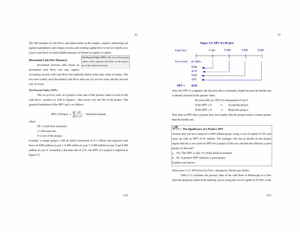
5.52

52

The full estimate of cash flows, described earlier in the chapter, requires subtracting out

capital expenditures and changes in non-cash working capital but it is far too volatile on a

year-to-year basis to yield reliable measures of returns on equity or capital.

Discounted Cash Flow Measures

Investment decision rules based on

discounted cash flows not only replace

accounting income with cash flows but explicitly factor in the time value of money. The

two most widely used discounted cash flows rules are net present value and the internal

rate of return.

Net Present Value (NPV)

The net present value of a project is the sum of the present values of each of the

cash flows—positive as well as negative—that occurs over the life of the project. The

general formulation of the NPV rule is as follows:

!

NPV of Project = CFt

(1+r)tt =1

t =N

" - Initial Investment

where

CFt = Cash flow in period t

r = Discount rate

N = Life of the project.

Consider a simple project, with an initial investment of $ 1 billion and expected cash

flows of $300 million in year 1, $ 400 million in year 2, $ 500 million in year 3 and $ 600

million in year 4. Assuming a discount rate of 12%, the NPV of a project is depicted in

figure 5.3:

Net Present Value (NPV): The sum of the present

values of the expected cash flows on the project,

net of the initial investment.

5.53

53

Once the NPV is computed, the decision rule is extremely simple because the hurdle rate

is already factored in the present value.

Decision Rule for NPV for Independent Projects

If the NPV > 0 ! Accept the project

If the NPV < 0 ! Reject the project

Note that an NPV that is greater than zero implies that the project makes a return greater

than the hurdle rate.

5.7. The Significance of a Positive NPV

Assume that you have analyzed a $100 million project using a cost of capital of 15% and

come up with an NPV of $1 million. The manager who has to decide on the project

argues that this is too small an NPV for a project of this size and that this indicates a poor

project. Is this true?

a. Yes. The NPV is only 1% of the initial investment.

b. No. A positive NPV indicates a good project.

Explain your answer.

Illustration 5.11: NPV from the Firm’s Standpoint: Bookscape Online

Table 5.13 calculates the present value of the cash flows to Bookscape as a firm

from the proposed online book ordering service using the cost of capital of 25.48% as the

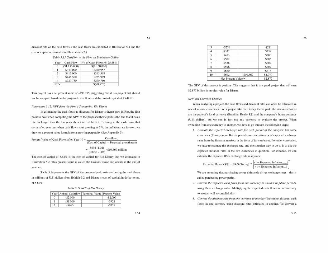
5.54

54

discount rate on the cash flows. (The cash flows are estimated in Illustration 5.4 and the

cost of capital is estimated in Illustration 5.2.)

Table 5.13 Cashflow to the Firm on Bookscape Online

Year Cash Flow PV of Cash Flows @ 25.48% 0 ($1,150,000) $(1,150,000) 1 $340,000 $270,957 2 $415,000 $263,568 3 $446,500 $225,989 4 $720,730 $290,710

NPV $(98,775)

This project has a net present value of –$98,775, suggesting that it is a project that should

not be accepted based on the projected cash flows and the cost of capital of 25.48%.

Illustration 5.12: NPV from the Firm’s Standpoint: Rio Disney

In estimating the cash flows to discount for Disney’s theme park in Rio, the first

point to note when computing the NPV of the proposed theme park is the fact that it has a

life far longer than the ten years shown in Exhibit 5.2. To bring in the cash flows that

occur after year ten, when cash flows start growing at 2%, the inflation rate forever, we

draw on a present value formula for a growing perpetuity (See Appendix 3):

Present Value of Cash Flows after Year 10 =

!

Cashflow11

(Cost of Capital - Perpetual growth rate)

=

!

$692 (1.02)(.0862 - .02)

=$10,669 million

The cost of capital of 8.62% is the cost of capital for Rio Disney that we estimated in

Illustration 5.2. This present value is called the terminal value and occurs at the end of

year ten.

Table 5.14 presents the NPV of the proposed park estimated using the cash flows

in millions of U.S. dollars from Exhibit 5.2 and Disney’s cost of capital, in dollar terms,

of 8.62%.

Table 5.14 NPV of Rio Disney

Year Annual Cashflow Terminal Value Present Value 0 -$2,000 -$2,000 1 -$1,000 -$921 2 -$860 -$729

5.55

55

3 -$270 -$211 4 $332 $239 5 $453 $300 6 $502 $305 7 $538 $302 8 $596 $307 9 $660 $313

10 $692 $10,669 $4,970 Net Present Value = $2,877

The NPV of this project is positive. This suggests that it is a good project that will earn

$2.877 billion in surplus value for Disney.

NPV and Currency Choices

When analyzing a project, the cash flows and discount rates can often be estimated in

one of several currencies. For a project like the Disney theme park, the obvious choices

are the project’s local currency (Brazilian Reals- R$) and the company’s home currency

(U.S. dollars), but we can in fact use any currency to evaluate the project. When

switching from one currency to another, we have to go through the following steps:

1. Estimate the expected exchange rate for each period of the analysis: For some

currencies (Euro, yen, or British pound), we can estimates of expected exchange

rates from the financial markets in the form of forward rates. For other currencies,

we have to estimate the exchange rate, and the soundest way to do so is to use the

expected inflation rates in the two currencies in question. For instance, we can

estimate the expected R$/$ exchange rate in n years:

Expected Rate (R$/$) =

!

$R/$ (Today) * (1+ Expected InflationBrazil )(1 + Expected InflationUS)

"

# $

%

& '

n

We are assuming that purchasing power ultimately drives exchange rates—this is

called purchasing power parity.

2. Convert the expected cash flows from one currency to another in future periods,

using these exchange rates: Multiplying the expected cash flows in one currency

to another will accomplish this.

3. Convert the discount rate from one currency to another: We cannot discount cash

flows in one currency using discount rates estimated in another. To convert a

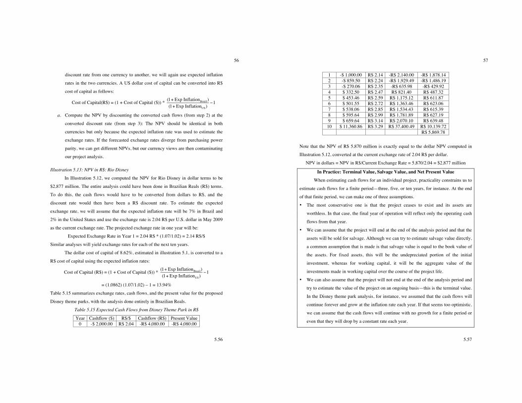
5.56

56

discount rate from one currency to another, we will again use expected inflation

rates in the two currencies. A US dollar cost of capital can be converted into R$

cost of capital as follows:

Cost of Capital(R$) = (1 + Cost of Capital ($)) *

!

(1+ Exp InflationBrazil)(1+ Exp InflationUS)

"1

a. Compute the NPV by discounting the converted cash flows (from step 2) at the

converted discount rate (from step 3): The NPV should be identical in both

currencies but only because the expected inflation rate was used to estimate the

exchange rates. If the forecasted exchange rates diverge from purchasing power

parity, we can get different NPVs, but our currency views are then contaminating

our project analysis.

Illustration 5.13: NPV in R$: Rio Disney

In Illustration 5.12, we computed the NPV for Rio Disney in dollar terms to be

$2,877 million. The entire analysis could have been done in Brazilian Reals (R$) terms.

To do this, the cash flows would have to be converted from dollars to R$, and the

discount rate would then have been a R$ discount rate. To estimate the expected

exchange rate, we will assume that the expected inflation rate will be 7% in Brazil and

2% in the United States and use the exchange rate is 2.04 R$ per U.S. dollar in May 2009

as the current exchange rate. The projected exchange rate in one year will be:

Expected Exchange Rate in Year 1 = 2.04 R$ * (1.07/1.02) = 2.14 R$/$

Similar analyses will yield exchange rates for each of the next ten years.

The dollar cost of capital of 8.62%, estimated in illustration 5.1, is converted to a

R$ cost of capital using the expected inflation rates:

Cost of Capital (R$) = (1 + Cost of Capital ($)) *

!

(1+ Exp InflationBrazil)(1+ Exp InflationUS)

"1

= (1.0862) (1.07/1.02) – 1 = 13.94%

Table 5.15 summarizes exchange rates, cash flows, and the present value for the proposed

Disney theme parks, with the analysis done entirely in Brazilian Reals.

Table 5.15 Expected Cash Flows from Disney Theme Park in R$

Year Cashflow ($) R$/$ Cashflow (R$) Present Value 0 -$ 2,000.00 R$ 2.04 -R$ 4,080.00 -R$ 4,080.00

5.57

57

1 -$ 1,000.00 R$ 2.14 -R$ 2,140.00 -R$ 1,878.14 2 -$ 859.50 R$ 2.24 -R$ 1,929.49 -R$ 1,486.19 3 -$ 270.06 R$ 2.35 -R$ 635.98 -R$ 429.92 4 $ 332.50 R$ 2.47 R$ 821.40 R$ 487.32 5 $ 453.46 R$ 2.59 R$ 1,175.12 R$ 611.87 6 $ 501.55 R$ 2.72 R$ 1,363.46 R$ 623.06 7 $ 538.06 R$ 2.85 R$ 1,534.43 R$ 615.39 8 $ 595.64 R$ 2.99 R$ 1,781.89 R$ 627.19 9 $ 659.64 R$ 3.14 R$ 2,070.10 R$ 639.48 10 $ 11,360.86 R$ 3.29 R$ 37,400.49 R$ 10,139.72 R$ 5,869.78

Note that the NPV of R$ 5,870 million is exactly equal to the dollar NPV computed in

Illustration 5.12, converted at the current exchange rate of 2.04 R$ per dollar.

NPV in dollars = NPV in R$/Current Exchange Rate = 5,870/2.04 = $2,877 million

In Practice: Terminal Value, Salvage Value, and Net Present Value

When estimating cash flows for an individual project, practicality constrains us to

estimate cash flows for a finite period—three, five, or ten years, for instance. At the end

of that finite period, we can make one of three assumptions.

• The most conservative one is that the project ceases to exist and its assets are

worthless. In that case, the final year of operation will reflect only the operating cash

flows from that year.

• We can assume that the project will end at the end of the analysis period and that the

assets will be sold for salvage. Although we can try to estimate salvage value directly,

a common assumption that is made is that salvage value is equal to the book value of

the assets. For fixed assets, this will be the undepreciated portion of the initial

investment, whereas for working capital, it will be the aggregate value of the

investments made in working capital over the course of the project life.

• We can also assume that the project will not end at the end of the analysis period and

try to estimate the value of the project on an ongoing basis—this is the terminal value.

In the Disney theme park analysis, for instance, we assumed that the cash flows will

continue forever and grow at the inflation rate each year. If that seems too optimistic,

we can assume that the cash flows will continue with no growth for a finite period or

even that they will drop by a constant rate each year.

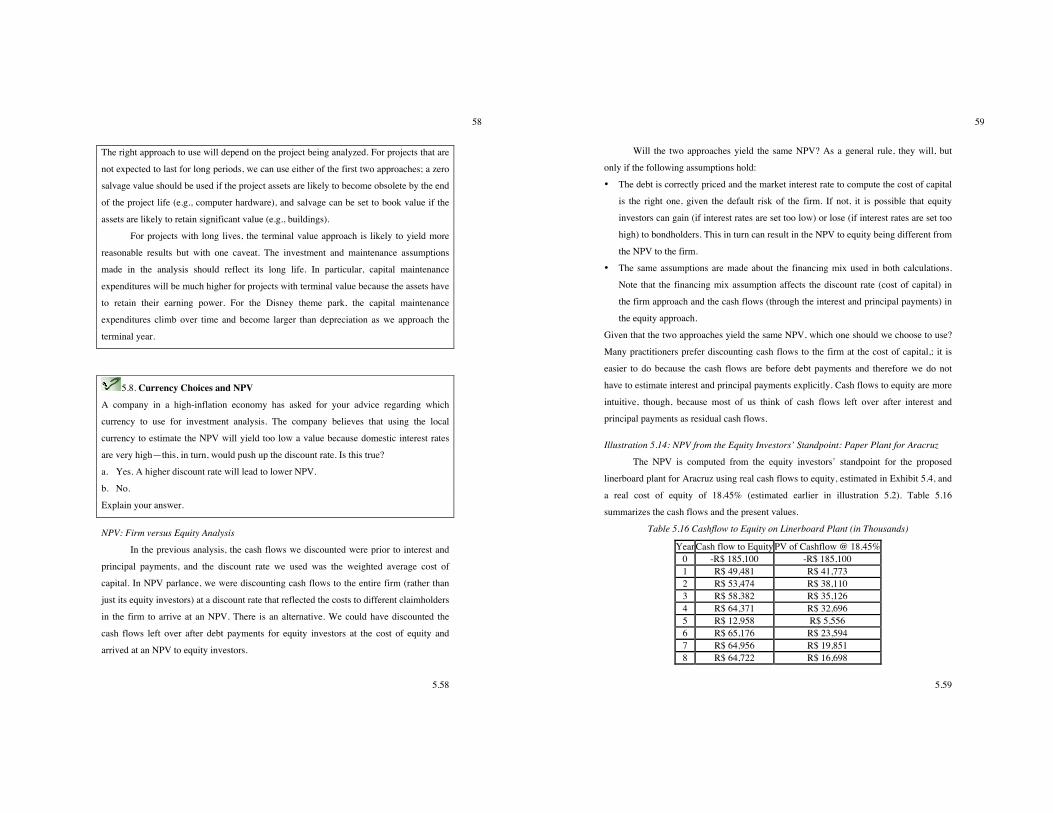
5.58

58

The right approach to use will depend on the project being analyzed. For projects that are

not expected to last for long periods, we can use either of the first two approaches; a zero

salvage value should be used if the project assets are likely to become obsolete by the end

of the project life (e.g., computer hardware), and salvage can be set to book value if the

assets are likely to retain significant value (e.g., buildings).

For projects with long lives, the terminal value approach is likely to yield more

reasonable results but with one caveat. The investment and maintenance assumptions

made in the analysis should reflect its long life. In particular, capital maintenance

expenditures will be much higher for projects with terminal value because the assets have

to retain their earning power. For the Disney theme park, the capital maintenance

expenditures climb over time and become larger than depreciation as we approach the

terminal year.

5.8. Currency Choices and NPV

A company in a high-inflation economy has asked for your advice regarding which

currency to use for investment analysis. The company believes that using the local

currency to estimate the NPV will yield too low a value because domestic interest rates

are very high—this, in turn, would push up the discount rate. Is this true?

a. Yes. A higher discount rate will lead to lower NPV.

b. No.

Explain your answer.

NPV: Firm versus Equity Analysis

In the previous analysis, the cash flows we discounted were prior to interest and

principal payments, and the discount rate we used was the weighted average cost of

capital. In NPV parlance, we were discounting cash flows to the entire firm (rather than

just its equity investors) at a discount rate that reflected the costs to different claimholders

in the firm to arrive at an NPV. There is an alternative. We could have discounted the

cash flows left over after debt payments for equity investors at the cost of equity and

arrived at an NPV to equity investors.

5.59

59

Will the two approaches yield the same NPV? As a general rule, they will, but

only if the following assumptions hold:

• The debt is correctly priced and the market interest rate to compute the cost of capital

is the right one, given the default risk of the firm. If not, it is possible that equity

investors can gain (if interest rates are set too low) or lose (if interest rates are set too

high) to bondholders. This in turn can result in the NPV to equity being different from

the NPV to the firm.

• The same assumptions are made about the financing mix used in both calculations.

Note that the financing mix assumption affects the discount rate (cost of capital) in

the firm approach and the cash flows (through the interest and principal payments) in

the equity approach.

Given that the two approaches yield the same NPV, which one should we choose to use?

Many practitioners prefer discounting cash flows to the firm at the cost of capital,; it is

easier to do because the cash flows are before debt payments and therefore we do not

have to estimate interest and principal payments explicitly. Cash flows to equity are more

intuitive, though, because most of us think of cash flows left over after interest and

principal payments as residual cash flows.

Illustration 5.14: NPV from the Equity Investors’ Standpoint: Paper Plant for Aracruz

The NPV is computed from the equity investors’ standpoint for the proposed

linerboard plant for Aracruz using real cash flows to equity, estimated in Exhibit 5.4, and

a real cost of equity of 18.45% (estimated earlier in illustration 5.2). Table 5.16

summarizes the cash flows and the present values.

Table 5.16 Cashflow to Equity on Linerboard Plant (in Thousands)

Year Cash flow to Equity PV of Cashflow @ 18.45% 0 -R$ 185,100 -R$ 185,100 1 R$ 49,481 R$ 41,773 2 R$ 53,474 R$ 38,110 3 R$ 58,382 R$ 35,126 4 R$ 64,371 R$ 32,696 5 R$ 12,958 R$ 5,556 6 R$ 65,176 R$ 23,594 7 R$ 64,956 R$ 19,851 8 R$ 64,722 R$ 16,698

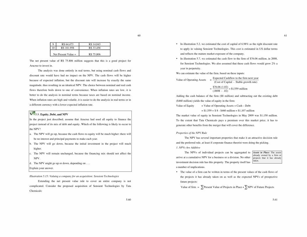
5.60

60

9 R$ 64,473 R$ 14,043 10 R$ 181,958 R$ 33,458

Net Present Value = R$ 75,806

The net present value of R$ 75.806 million suggests that this is a good project for

Aracruz to invest in.

The analysis was done entirely in real terms, but using nominal cash flows and

discount rate would have had no impact on the NPV. The cash flows will be higher

because of expected inflation, but the discount rate will increase by exactly the same

magnitude, thus resulting in an identical NPV. The choice between nominal and real cash

flows therefore boils down to one of convenience. When inflation rates are low, it is

better to do the analysis in nominal terms because taxes are based on nominal income.

When inflation rates are high and volatile, it is easier to do the analysis in real terms or in

a different currency with a lower expected inflation rate.

5.9. Equity, Debt, and NPV

In the project just described, assume that Aracruz had used all equity to finance the

project instead of its mix of debt and equity. Which of the following is likely to occur to

the NPV?

a. The NPV will go up, because the cash flows to equity will be much higher; there will

be no interest and principal payments to make each year.

b. The NPV will go down, because the initial investment in the project will much

higher.

c. The NPV will remain unchanged, because the financing mix should not affect the

NPV.

d. The NPV might go up or down, depending on . . .

Explain your answer.

Illustration 5.15: Valuing a company for an acquisition: Sensient Technologies

Extending the net present value rule to cover an entire company is not

complicated. Consider the proposed acquisition of Sensient Technologies by Tata

Chemicals:

5.61

61

• In illustration 5.2, we estimated the cost of capital of 6.98% as the right discount rate

to apply in valuing Sensient Technologies. This cost is estimated in US dollar terms

and reflects the mature market exposure of the company.

• In illustration 5.7, we estimated the cash flow to the firm of $76.06 million, in 2008,

for Sensient Technologies. We also assumed that these cash flows would grow 2% a

year in perpetuity.

We can estimate the value of the firm, based on these inputs:

Value of Operating Assets =

!

Expected Cashflow to the firm next year(Cost of Capital - Stable growth rate)

=

!

$76.06 (1.02)(.0698 - .02)

= $1,559 million

Adding the cash balance of the firm ($8 million) and subtracting out the existing debt

($460 million) yields the value of equity in the firm:

Value of Equity = Value of Operating Assets + Cash – Debt

= $1,559 + $ 8 - $460 million = $1,107 million

The market value of equity in Sensient Technologies in May 2009 was $1,150 million.

To the extent that Tata Chemicals pays a premium over this market price, it has to

generate other benefits from the merger that will cover the difference.

Properties of the NPV Rule

The NPV has several important properties that make it an attractive decision rule

and the preferred rule, at least if corporate finance theorist were doing the picking.

1. NPVs Are Additive

The NPVs of individual projects can be aggregated to

arrive at a cumulative NPV for a business or a division. No other

investment decision rule has this property. The property itself has

a number of implications.

• The value of a firm can be written in terms of the present values of the cash flows of

the projects it has already taken on as well as the expected NPVs of prospective

future projects:

!

Value of firm = Present Value of Projects in Place + NPV of Future Projects""

Assets in Place: The assets already owned by a firm or projects that it has already taken.

5.62

62

The first term in this equation captures the value of assets in place, whereas the

second term measures the value of expected future growth. Note that the present value

of projects in place is based on anticipated future cash flows on these projects.

• When a firm terminates an existing project that has a negative present value based on

anticipated future cash flows, the value of the firm will increase by that amount.

Similarly, when a invests in a new project, with an expected negative NPV, the value

of the firm will decrease by that amount.

• When a firm divests itself of an existing asset, the price received for that asset will

affect the value of the firm. If the price received exceeds the present value of the

anticipated cash flows on that project to the firm, the value of the firm will increase

with the divestiture; otherwise, it will decrease.

• When a firm invests in a new project with a positive NPV, the value of the firm will

be affected depending on whether the NPV meets expectations. For example, a firm

like Microsoft is expected to take on high positive NPV projects, and this expectation

is built into value. Even if the new projects taken on by Microsoft have positive NPV,

there may be a drop in value if the NPV does not meet the high expectations of

financial markets.

• When a firm makes an acquisition and pays a price that exceeds the present value of

the expected cash flows from the firm being acquired, it is the equivalent of taking on

a negative NPV project and will lead to a drop in value.

5.10. Firm Value and Overpayment on Acquisitions Megatech Corporation, a large software firm with a market value for its equity of $100

million, announces that it will be acquiring FastMail Corporation, a smaller software

firm, for $15 million. On the announcement, Megatech’s stock price drops by 3%. Based

on these facts, estimate the amount the market thinks Megatech should have paid for

FastMail.

a. $15 million

b. $3 million

c. $12 million

How does NPV additivity enter into your answer?

5.63

63

2. Intermediate Cash Flows Are Invested at the Hurdle Rate

Implicit in all present value calculations are assumptions about the rate at which

intermediate cash flows get reinvested. The NPV

rule assumes that intermediate cash flows on a

projects—that is, cash flows that occur between

the initiation and the end of the project—get

reinvested at the hurdle rate, which is the cost of capital if the cash flows are to the firm

and the cost of equity if the cash flows are to equity investors. Given that both the cost of

equity and capital are based on the returns that can be made on alternative investments of

equivalent risk, this assumption should be reasonable.

3. NPV Calculations Allow for Expected Term Structure and Interest Rate Shifts

In all the examples throughout in this chapter, we have assumed that the discount

rate remains unchanged over time. This is not always the case, however; the NPV can be

computed using time-varying discount rates. The general formulation for the NPV rule is

as follows:

NPV of Project = CFt

j=1

j= t

! (1 + rt )t=1

t = N

" - Initial Investment

where

CFt = Cash flow in period t

rt = One-period discount rate that applies to period t

N = Life of the project.

The discount rates may change for three reasons:

• The level of interest rates may change over time, and the term structure may provide

some insight on expected rates in the future.

• The risk characteristics of the project may be expected to change in a predictable way

over time, resulting in changes in the discount rate.

• The financing mix on the project may change over time, resulting in changes in both

the cost of equity and the cost of capital.

Hurdle Rate: The minimum acceptable rate

of return that a firm will accept for taking a

given project.

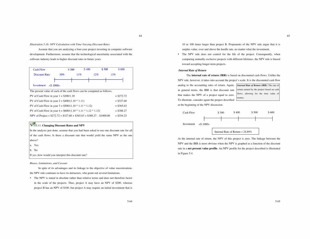
5.64

64

Illustration 5.16: NPV Calculation with Time-Varying Discount Rates

Assume that you are analyzing a four-year project investing in computer software

development. Furthermore, assume that the technological uncertainty associated with the

software industry leads to higher discount rates in future years.

The present value of each of the cash flows can be computed as follows.

PV of Cash Flow in year 1 = $300/1.10 = $272.72

PV of Cash Flow in year 2 = $400/(1.10 * 1.11) = $327.60

PV of Cash Flow in year 3 = $500/(1.10 * 1.11 * 1.12) = $365.63

PV of Cash Flow in year 4 = $600/(1.10 * 1.11 * 1.12 * 1.13) = $388.27

NPV of Project = $272.72 + $327.60 + $365.63 + $388.27 – $1000.00 = $354.23

5.11. Changing Discount Rates and NPV In the analysis just done, assume that you had been asked to use one discount rate for all

of the cash flows. Is there a discount rate that would yield the same NPV as the one

above?

a. Yes

b. No

If yes, how would you interpret this discount rate?

Biases, Limitations, and Caveats

In spite of its advantages and its linkage to the objective of value maximization,

the NPV rule continues to have its detractors, who point out several limitations.

• The NPV is stated in absolute rather than relative terms and does not therefore factor

in the scale of the projects. Thus, project A may have an NPV of $200, whereas

project B has an NPV of $100, but project A may require an initial investment that is

5.65

65

10 or 100 times larger than project B. Proponents of the NPV rule argue that it is

surplus value, over and above the hurdle rate, no matter what the investment.

• The NPV rule does not control for the life of the project. Consequently, when

comparing mutually exclusive projects with different lifetimes, the NPV rule is biased

toward accepting longer-term projects.

Internal Rate of Return

The internal rate of return (IRR) is based on discounted cash flows. Unlike the

NPV rule, however, it takes into account the project’s scale. It is the discounted cash flow

analog to the accounting rates of return. Again,

in general terms, the IRR is that discount rate

that makes the NPV of a project equal to zero.

To illustrate, consider again the project described

at the beginning of the NPV discussion.

Cash Flow

Investment

$ 300 $ 400 $ 500 $ 600

<$ 1000>

Internal Rate of Return = 24.89%

At the internal rate of return, the NPV of this project is zero. The linkage between the

NPV and the IRR is most obvious when the NPV is graphed as a function of the discount

rate in a net present value profile. An NPV profile for the project described is illustrated

in Figure 5.4.

Internal Rate of Return (IRR): The rate of

return earned by the project based on cash

flows, allowing for the time value of

money.

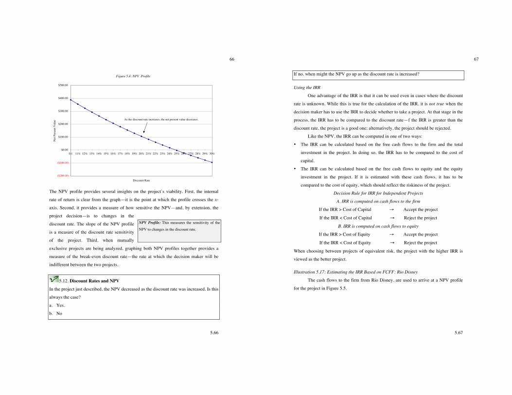
5.66

66

Figure 5.4: NPV Profile

($200.00)

($100.00)

$0.00

$100.00

$200.00

$300.00

$400.00

$500.00

0.1 11% 12% 13% 14% 15% 16% 17% 18% 19% 20% 21% 22% 23% 24% 25% 26% 27% 28% 29% 30%

Discount Rate

Net

Pre

sent

Val

ue

As the discount rate increases, the net present value decreases.

The NPV profile provides several insights on the project’s viability. First, the internal

rate of return is clear from the graph—it is the point at which the profile crosses the x-

axis. Second, it provides a measure of how sensitive the NPV—and, by extension, the

project decision—is to changes in the

discount rate. The slope of the NPV profile

is a measure of the discount rate sensitivity

of the project. Third, when mutually

exclusive projects are being analyzed, graphing both NPV profiles together provides a

measure of the break-even discount rate—the rate at which the decision maker will be

indifferent between the two projects.

5.12. Discount Rates and NPV

In the project just described, the NPV decreased as the discount rate was increased. Is this

always the case?

a. Yes.

b. No

NPV Profile: This measures the sensitivity of the

NPV to changes in the discount rate.

5.67

67

If no, when might the NPV go up as the discount rate is increased?

Using the IRR

One advantage of the IRR is that it can be used even in cases where the discount

rate is unknown. While this is true for the calculation of the IRR, it is not true when the

decision maker has to use the IRR to decide whether to take a project. At that stage in the

process, the IRR has to be compared to the discount rate—f the IRR is greater than the

discount rate, the project is a good one; alternatively, the project should be rejected.

Like the NPV, the IRR can be computed in one of two ways:

• The IRR can be calculated based on the free cash flows to the firm and the total

investment in the project. In doing so, the IRR has to be compared to the cost of

capital.

• The IRR can be calculated based on the free cash flows to equity and the equity

investment in the project. If it is estimated with these cash flows, it has to be

compared to the cost of equity, which should reflect the riskiness of the project.

Decision Rule for IRR for Independent Projects

A. IRR is computed on cash flows to the firm

If the IRR > Cost of Capital ! Accept the project

If the IRR < Cost of Capital ! Reject the project

B. IRR is computed on cash flows to equity

If the IRR > Cost of Equity ! Accept the project

If the IRR < Cost of Equity ! Reject the project

When choosing between projects of equivalent risk, the project with the higher IRR is

viewed as the better project.

Illustration 5.17: Estimating the IRR Based on FCFF: Rio Disney

The cash flows to the firm from Rio Disney, are used to arrive at a NPV profile

for the project in Figure 5.5.

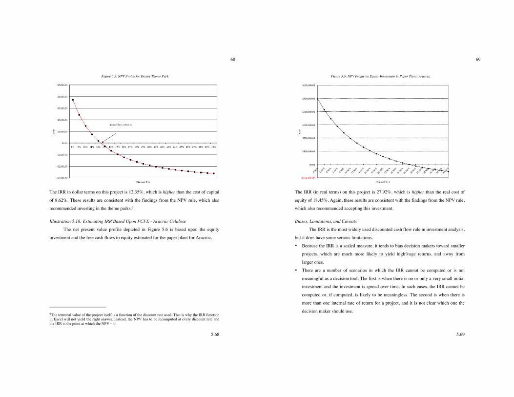
5.68

68

The IRR in dollar terms on this project is 12.35%, which is higher than the cost of capital

of 8.62%. These results are consistent with the findings from the NPV rule, which also

recommended investing in the theme parks.9

Illustration 5.18: Estimating IRR Based Upon FCFE - Aracruz Celulose

The net present value profile depicted in Figure 5.6 is based upon the equity

investment and the free cash flows to equity estimated for the paper plant for Aracruz.

9The terminal value of the project itself is a function of the discount rate used. That is why the IRR function in Excel will not yield the right answer. Instead, the NPV has to be recomputed at every discount rate and the IRR is the point at which the NPV = 0.

5.69

69

The IRR (in real terms) on this project is 27.92%, which is higher than the real cost of

equity of 18.45%. Again, these results are consistent with the findings from the NPV rule,

which also recommended accepting this investment.

Biases, Limitations, and Caveats

The IRR is the most widely used discounted cash flow rule in investment analysis,

but it does have some serious limitations.

• Because the IRR is a scaled measure, it tends to bias decision makers toward smaller

projects, which are much more likely to yield high%age returns, and away from

larger ones.

• There are a number of scenarios in which the IRR cannot be computed or is not

meaningful as a decision tool. The first is when there is no or only a very small initial

investment and the investment is spread over time. In such cases, the IRR cannot be

computed or, if computed, is likely to be meaningless. The second is when there is

more than one internal rate of return for a project, and it is not clear which one the

decision maker should use.

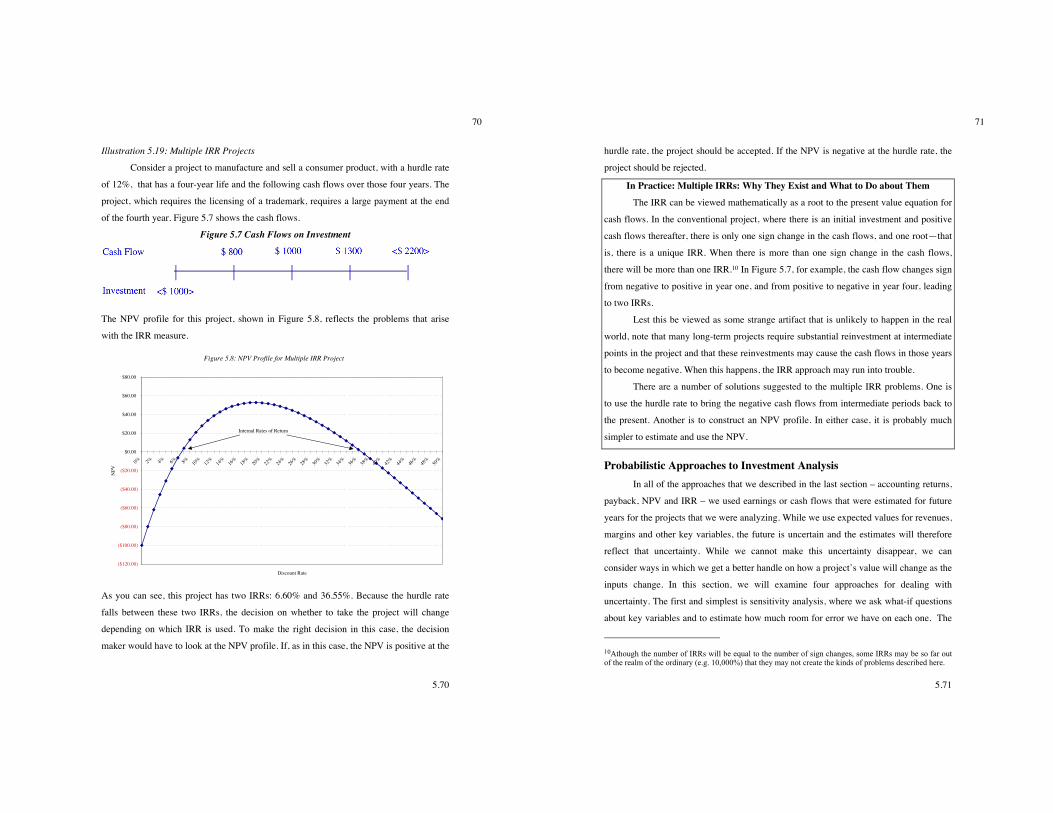
5.70

70

Illustration 5.19: Multiple IRR Projects

Consider a project to manufacture and sell a consumer product, with a hurdle rate

of 12%, that has a four-year life and the following cash flows over those four years. The

project, which requires the licensing of a trademark, requires a large payment at the end

of the fourth year. Figure 5.7 shows the cash flows.

Figure 5.7 Cash Flows on Investment

The NPV profile for this project, shown in Figure 5.8, reflects the problems that arise

with the IRR measure.

Figure 5.8: NPV Profile for Multiple IRR Project

($120.00)

($100.00)

($80.00)

($60.00)

($40.00)

($20.00)

$0.00

$20.00

$40.00

$60.00

$80.00

0% 2% 4% 6% 8% 10%

12%

14%

16%

18%

20%

22%

24%

26%

28%

30%

32%

34%

36%

38%

40%

42%

44%

46%

48%

50%

Discount Rate

NPV

Internal Rates of Return

As you can see, this project has two IRRs: 6.60% and 36.55%. Because the hurdle rate

falls between these two IRRs, the decision on whether to take the project will change

depending on which IRR is used. To make the right decision in this case, the decision

maker would have to look at the NPV profile. If, as in this case, the NPV is positive at the

5.71

71

hurdle rate, the project should be accepted. If the NPV is negative at the hurdle rate, the

project should be rejected.

In Practice: Multiple IRRs: Why They Exist and What to Do about Them The IRR can be viewed mathematically as a root to the present value equation for

cash flows. In the conventional project, where there is an initial investment and positive

cash flows thereafter, there is only one sign change in the cash flows, and one root—that

is, there is a unique IRR. When there is more than one sign change in the cash flows,

there will be more than one IRR.10 In Figure 5.7, for example, the cash flow changes sign

from negative to positive in year one, and from positive to negative in year four, leading

to two IRRs.

Lest this be viewed as some strange artifact that is unlikely to happen in the real

world, note that many long-term projects require substantial reinvestment at intermediate

points in the project and that these reinvestments may cause the cash flows in those years

to become negative. When this happens, the IRR approach may run into trouble.

There are a number of solutions suggested to the multiple IRR problems. One is

to use the hurdle rate to bring the negative cash flows from intermediate periods back to

the present. Another is to construct an NPV profile. In either case, it is probably much

simpler to estimate and use the NPV.

Probabilistic Approaches to Investment Analysis In all of the approaches that we described in the last section – accounting returns,

payback, NPV and IRR – we used earnings or cash flows that were estimated for future

years for the projects that we were analyzing. While we use expected values for revenues,

margins and other key variables, the future is uncertain and the estimates will therefore

reflect that uncertainty. While we cannot make this uncertainty disappear, we can

consider ways in which we get a better handle on how a project’s value will change as the

inputs change. In this section, we will examine four approaches for dealing with

uncertainty. The first and simplest is sensitivity analysis, where we ask what-if questions

about key variables and to estimate how much room for error we have on each one. The

10Athough the number of IRRs will be equal to the number of sign changes, some IRRs may be so far out of the realm of the ordinary (e.g. 10,000%) that they may not create the kinds of problems described here.

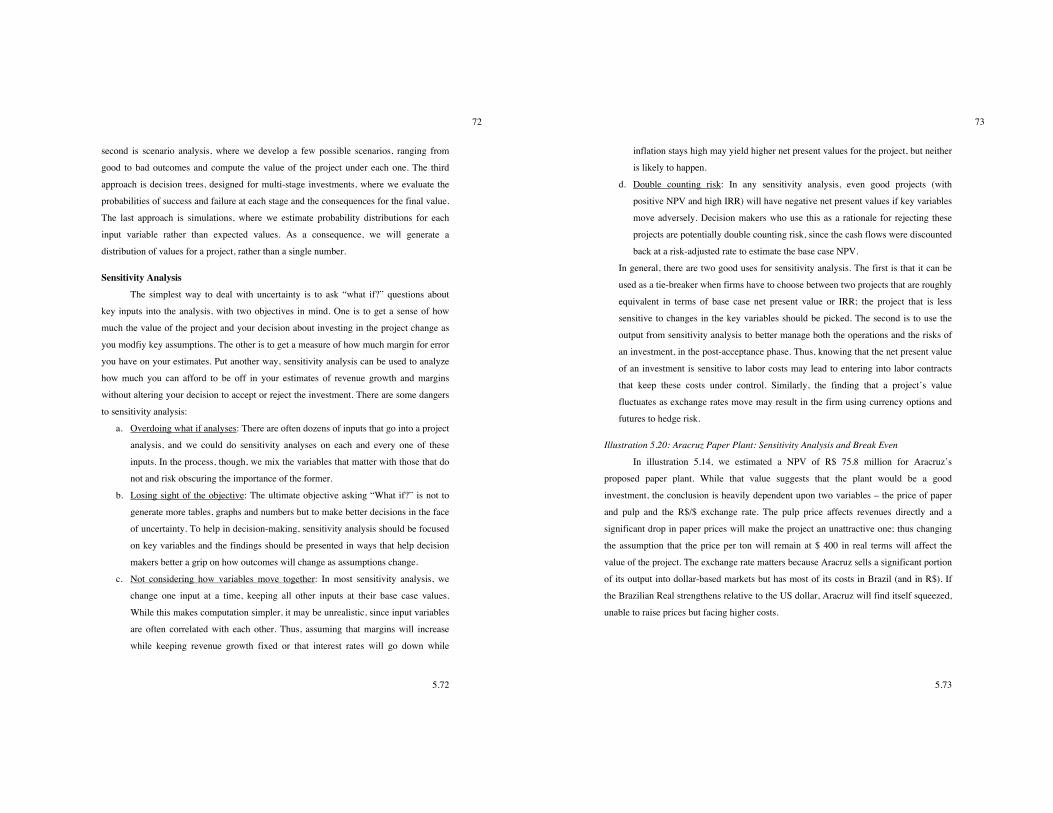
5.72

72

second is scenario analysis, where we develop a few possible scenarios, ranging from

good to bad outcomes and compute the value of the project under each one. The third

approach is decision trees, designed for multi-stage investments, where we evaluate the

probabilities of success and failure at each stage and the consequences for the final value.

The last approach is simulations, where we estimate probability distributions for each

input variable rather than expected values. As a consequence, we will generate a

distribution of values for a project, rather than a single number.

Sensitivity Analysis The simplest way to deal with uncertainty is to ask “what if?” questions about

key inputs into the analysis, with two objectives in mind. One is to get a sense of how

much the value of the project and your decision about investing in the project change as

you modfiy key assumptions. The other is to get a measure of how much margin for error

you have on your estimates. Put another way, sensitivity analysis can be used to analyze

how much you can afford to be off in your estimates of revenue growth and margins

without altering your decision to accept or reject the investment. There are some dangers

to sensitivity analysis:

a. Overdoing what if analyses: There are often dozens of inputs that go into a project

analysis, and we could do sensitivity analyses on each and every one of these

inputs. In the process, though, we mix the variables that matter with those that do

not and risk obscuring the importance of the former.

b. Losing sight of the objective: The ultimate objective asking “What if?” is not to

generate more tables, graphs and numbers but to make better decisions in the face

of uncertainty. To help in decision-making, sensitivity analysis should be focused

on key variables and the findings should be presented in ways that help decision

makers better a grip on how outcomes will change as assumptions change.

c. Not considering how variables move together: In most sensitivity analysis, we

change one input at a time, keeping all other inputs at their base case values.

While this makes computation simpler, it may be unrealistic, since input variables

are often correlated with each other. Thus, assuming that margins will increase

while keeping revenue growth fixed or that interest rates will go down while

5.73

73

inflation stays high may yield higher net present values for the project, but neither

is likely to happen.

d. Double counting risk: In any sensitivity analysis, even good projects (with

positive NPV and high IRR) will have negative net present values if key variables

move adversely. Decision makers who use this as a rationale for rejecting these

projects are potentially double counting risk, since the cash flows were discounted

back at a risk-adjusted rate to estimate the base case NPV.

In general, there are two good uses for sensitivity analysis. The first is that it can be

used as a tie-breaker when firms have to choose between two projects that are roughly

equivalent in terms of base case net present value or IRR; the project that is less

sensitive to changes in the key variables should be picked. The second is to use the

output from sensitivity analysis to better manage both the operations and the risks of

an investment, in the post-acceptance phase. Thus, knowing that the net present value

of an investment is sensitive to labor costs may lead to entering into labor contracts

that keep these costs under control. Similarly, the finding that a project’s value

fluctuates as exchange rates move may result in the firm using currency options and

futures to hedge risk.

Illustration 5.20: Aracruz Paper Plant: Sensitivity Analysis and Break Even

In illustration 5.14, we estimated a NPV of R$ 75.8 million for Aracruz’s

proposed paper plant. While that value suggests that the plant would be a good

investment, the conclusion is heavily dependent upon two variables – the price of paper

and pulp and the R$/$ exchange rate. The pulp price affects revenues directly and a

significant drop in paper prices will make the project an unattractive one; thus changing

the assumption that the price per ton will remain at $ 400 in real terms will affect the

value of the project. The exchange rate matters because Aracruz sells a significant portion

of its output into dollar-based markets but has most of its costs in Brazil (and in R$). If

the Brazilian Real strengthens relative to the US dollar, Aracruz will find itself squeezed,

unable to raise prices but facing higher costs.

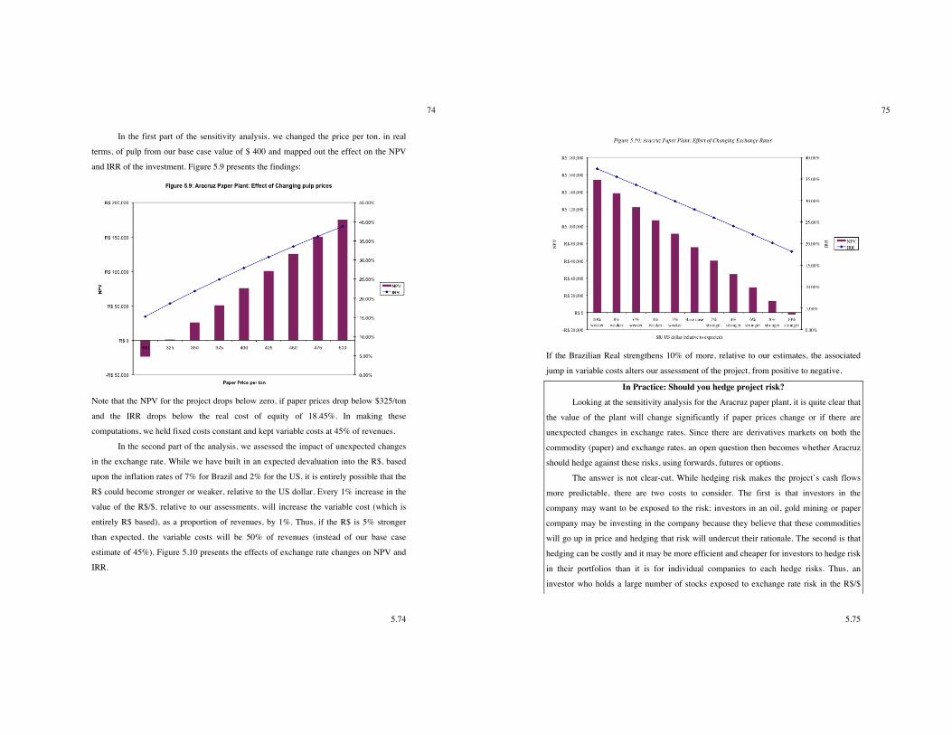
5.74

74

In the first part of the sensitivity analysis, we changed the price per ton, in real

terms, of pulp from our base case value of $ 400 and mapped out the effect on the NPV

and IRR of the investment. Figure 5.9 presents the findings:

Note that the NPV for the project drops below zero, if paper prices drop below $325/ton

and the IRR drops below the real cost of equity of 18.45%. In making these

computations, we held fixed costs constant and kept variable costs at 45% of revenues.

In the second part of the analysis, we assessed the impact of unexpected changes

in the exchange rate. While we have built in an expected devaluation into the R$, based

upon the inflation rates of 7% for Brazil and 2% for the US, it is entirely possible that the

R$ could become stronger or weaker, relative to the US dollar. Every 1% increase in the

value of the R$/$, relative to our assessments, will increase the variable cost (which is

entirely R$ based), as a proportion of revenues, by 1%. Thus, if the R$ is 5% stronger

than expected, the variable costs will be 50% of revenues (instead of our base case

estimate of 45%). Figure 5.10 presents the effects of exchange rate changes on NPV and

IRR.

5.75

75

If the Brazilian Real strengthens 10% of more, relative to our estimates, the associated

jump in variable costs alters our assessment of the project, from positive to negative.

In Practice: Should you hedge project risk? Looking at the sensitivity analysis for the Aracruz paper plant, it is quite clear that

the value of the plant will change significantly if paper prices change or if there are

unexpected changes in exchange rates. Since there are derivatives markets on both the

commodity (paper) and exchange rates, an open question then becomes whether Aracruz

should hedge against these risks, using forwards, futures or options.

The answer is not clear-cut. While hedging risk makes the project’s cash flows

more predictable, there are two costs to consider. The first is that investors in the

company may want to be exposed to the risk; investors in an oil, gold mining or paper

company may be investing in the company because they believe that these commodities

will go up in price and hedging that risk will undercut their rationale. The second is that

hedging can be costly and it may be more efficient and cheaper for investors to hedge risk

in their portfolios than it is for individual companies to each hedge risks. Thus, an

investor who holds a large number of stocks exposed to exchange rate risk in the R$/$

5.76

76

rate may be able to diversify away a large component of that risk in his portfolio and then

can choose to hedge or not hedge the remaining risk. These costs have to be weighed

against two potential benefits. The first is that hedging against risks that can cause large

losses, relative to the size of the firm, may reduce the chance of default, especially if a

firm has significant debt obligations. The second is that hedging risk can sometimes yield

tax benefits, both in the form of tax-deductible expenses for hedging and from smoothing

out earnings.

Applying this trade off to Aracruz, we come to a mixed conclusion. The firm has

significant debt obligations and cannot risk large losses. Consequently, we think it makes

sense for the firm to hedge exchange rate risk, especially because it is relatively

inexpensive to do so, using futures and forward contracts. Given that it is a commodity

company, we are reluctant to suggest the same path for paper prices, since investors in

the company may want that exposure. One compromise that will allow these investors to

retain the upside, while protecting against very adverse moves in pulp prices, would be

for Aracruz to buy put options on paper at a price of around $325 (the breakeven point

for NPV). Since the put options will be deep out of the money, the costs should be

moderate and investors will still get most of the upside on paper prices.

Scenario Analysis In sensitivity analysis, we change one input variable at a time and examine the

effect on the output variables – NPV, IRR and accounting returns. In scenario analysis,

we outline scenarios that are different from the base case, where many or all of the inputs

can have different values, and evaluate the project’s value under these scenarios. In

general, scenario analysis can take one of two forms: a best case/worst case analysis or an

analysis of multiple possible scenarios.

Best Case, Worst Case

With risky projects, the actual cash flows can be very different from expectations.

At the minimum, we can estimate the cash flows if everything works to perfection – a

best case scenario – and if nothing does – a worse case scenario. In practice, there are two

ways in which this analysis can be structured. In the first, each input into the project

analysis is set to its best (or worst) possible outcome and the cash flows estimated with

5.77

77

those values. Thus, when analyzing a project, you may set the revenue growth rate and

operating margin at the highest possible level while setting the discount rate at its lowest

level, and compute the value as the best-case scenario. The problem with this approach is

that it may not be feasible; after all, to get the high revenue growth, the firm may have to

lower prices and accept lower margins. In the second, the best possible scenario is

defined in terms of what is feasible while allowing for the relationship between the

inputs. Thus, instead of assuming that revenue growth and margins will both be

maximized, we will choose that combination of growth and margin that is feasible and

yields the maximum value. While this approach is more realistic, it does require more

work to put into practice.

There are two ways in which the results from this analysis can help decision

makers. First, the difference between the best case and worst case value can be used as a

measure of risk on an asset; the range in value (scaled to size) should be higher for riskier

investments. Second, firms that are concerned about the potential spill over effects on

their operations of an investment going bad may be able to gauge the effects by looking

at the worst case outcome. Thus, a firm that has significant debt obligations may use the

worst case outcome to make a judgment as to whether an investment has the potential to

push them into default. In general, though, best case/worse case analyses are not very

informative. After all, there should be no surprise in knowing that an investment is worth

a great deal in the best case and does badly in the worst case.

Multiple Scenario Analysis

Scenario analysis does not have to be restricted to the best and worst cases. In its

most general form, the value of a risky investment can be computed under a number of

different scenarios, varying the assumptions about both macro economic and asset-

specific variables. While the concept of sensitivity analysis is a simple one, it has four

critical components:

• The first is the determination of which factors the scenarios will be built around.

These factors can range from the state of the economy for an automobile firm

considering a new plant, to the response of competitors for a consumer product firm

introducing a new product, to the behavior of regulatory authorities for a phone

company, considering a new phone service.

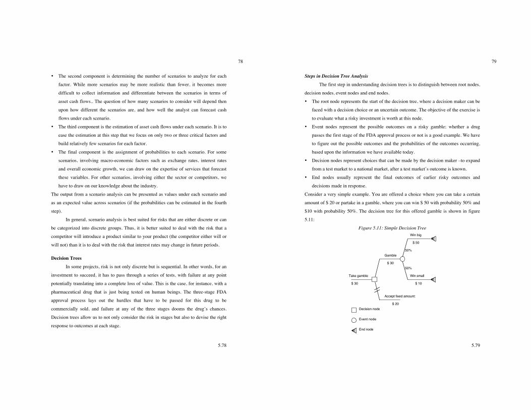
5.78

78

• The second component is determining the number of scenarios to analyze for each

factor. While more scenarios may be more realistic than fewer, it becomes more

difficult to collect information and differentiate between the scenarios in terms of

asset cash flows.. The question of how many scenarios to consider will depend then

upon how different the scenarios are, and how well the analyst can forecast cash

flows under each scenario.

• The third component is the estimation of asset cash flows under each scenario. It is to

ease the estimation at this step that we focus on only two or three critical factors and

build relatively few scenarios for each factor.

• The final component is the assignment of probabilities to each scenario. For some

scenarios, involving macro-economic factors such as exchange rates, interest rates

and overall economic growth, we can draw on the expertise of services that forecast

these variables. For other scenarios, involving either the sector or competitors, we

have to draw on our knowledge about the industry.

The output from a scenario analysis can be presented as values under each scenario and

as an expected value across scenarios (if the probabilities can be estimated in the fourth

step).

In general, scenario analysis is best suited for risks that are either discrete or can

be categorized into discrete groups. Thus, it is better suited to deal with the risk that a

competitor will introduce a product similar to your product (the competitor either will or

will not) than it is to deal with the risk that interest rates may change in future periods.

Decision Trees

In some projects, risk is not only discrete but is sequential. In other words, for an

investment to succeed, it has to pass through a series of tests, with failure at any point

potentially translating into a complete loss of value. This is the case, for instance, with a

pharmaceutical drug that is just being tested on human beings. The three-stage FDA

approval process lays out the hurdles that have to be passed for this drug to be

commercially sold, and failure at any of the three stages dooms the drug’s chances.

Decision trees allow us to not only consider the risk in stages but also to devise the right

response to outcomes at each stage.

5.79

79

Steps in Decision Tree Analysis

The first step in understanding decision trees is to distinguish between root nodes,

decision nodes, event nodes and end nodes.

• The root node represents the start of the decision tree, where a decision maker can be

faced with a decision choice or an uncertain outcome. The objective of the exercise is

to evaluate what a risky investment is worth at this node.

• Event nodes represent the possible outcomes on a risky gamble; whether a drug

passes the first stage of the FDA approval process or not is a good example. We have

to figure out the possible outcomes and the probabilities of the outcomes occurring,

based upon the information we have available today.

• Decision nodes represent choices that can be made by the decision maker –to expand

from a test market to a national market, after a test market’s outcome is known.

• End nodes usually represent the final outcomes of earlier risky outcomes and

decisions made in response.

Consider a very simple example. You are offered a choice where you can take a certain

amount of $ 20 or partake in a gamble, where you can win $ 50 with probability 50% and

$10 with probability 50%. The decision tree for this offered gamble is shown in figure

5.11:

Figure 5.11: Simple Decision Tree

Take gamble

Accept fixed amount:

$ 20

Gamble

$ 30

Win big

Win small

$ 50

$ 10$ 30

50%

50%

Decision node

Event node

End node

5.80

80

Note the key elements in the decision tree. First, only the event nodes represent uncertain

outcomes and have probabilities attached to them. Second, the decision node represents a

choice. On a pure expected value basis, the gamble is better (with an expected value of $

30) than the guaranteed amount of $20; the double slash on the latter branch indicates

that it would not be selected. While this example may be simplistic, the elements of

building a decision tree are in it.

Step 1: Divide analysis into risk phases: The key to developing a decision tree is

outlining the phases of risk that you will be exposed to in the future. In some cases, such

as the FDA approval process, this will be easy to do since there are only two outcomes –

the drug gets approved to move on to the next phase or it does not. In other cases, it will

be more difficult. For instance, a test market of a new consumer product can yield

hundreds of potential outcomes; here, you will have to create discrete categories for the

success of the test market.

Step 2: In each phase, estimate the probabilities of the outcomes: Once the phases of risk

have been put down and the outcomes at each phase are defined, the probabilities of the

outcomes have to be computed. In addition to the obvious requirement that the

probabilities across outcomes has to sum up to one, the analyst will also have to consider

whether the probabilities of outcomes in one phase can be affected by outcomes in earlier

phases. For example, how does the probability of a successful national product

introduction change when the test market outcome is only average?

Step 3: Define decision points: Embedded in the decision tree will be decision points

where you will get to determine, based upon observing the outcomes at earlier stages, and

expectations of what will occur in the future, what your best course of action will be.

With the test market example, for instance, you will get to determine, at the end of the

test market, whether you want to conduct a second test market, abandon the product or

move directly to a national product introduction.

Step 4: Compute cash flows/value at end nodes: The next step in the decision tree process

is estimating what the final cash flow and value outcomes will be at each end node. In

some cases, such as abandonment of a test market product, this will be easy to do and

will represent the money spent on the test marketing of the product. In other cases, such

as a national launch of the same product, this will be more difficult to do since you will

5.81

81

have to estimate expected cash flows over the life of the product and discount these cash

flows to arrive at value.

Step 5: Folding back the tree: The last step in a decision tree analysis is termed “folding

back’ the tree, where the expected values are computed working backwards through the

tree. If the node is a chance node, the expected value is computed as the probability

weighted average of all of the possible outcomes. If it is a decision node, the expected

value is computed for each branch, and the highest value is chosen (as the optimal

decision). The process culminates in an expected value for the asset or investment

today.11

There are two key pieces of output that emerge from a decision tree. The first is the

expected value today of going through the entire decision tree. This expected value will

incorporate the potential upside and downside from risk and the actions that you will take

along the way in response to this risk. In effect, this is analogous to the risk adjusted

value that we talked about in the last chapter. The second is the range of values at the end

nodes, which should encapsulate the potential risk in the investment.

Use in Decision Making

There are several benefits that accrue from using decision trees and it is surprising

that they are not used more often in analysis.

1. Dynamic response to Risk: By linking actions and choices to outcomes of uncertain

events, decision trees encourage firms to consider how they should act under different

circumstances. As a consequence, firms will be prepared for whatever outcome may

arise rather than be surprised. In the example in the last section, for instance, the firm

will be ready with a plan of action, no matter what the outcome of phase 3 happens to

be.

2. Value of Information: Decision trees provide a useful perspective on the value of

information in decision making. While it is not as obvious in the drug development

example, it can be seen clearly when a firm considers whether to test market a

product before commercially developing it. By test marketing a product, you acquire

11 There is a significant body of literature examining the assumptions that have to hold for this folding back process to yield consistent values. In particular, if a decision tree is used to portray concurrent risks, the

5.82

82

more information on the chances of eventual success. We can measure the expected

value of this improved information in a decision tree and compare it to the test

marketing cost.

3. Risk Management: Since decision trees provide a picture of how cash flows unfold

over time, they are useful in deciding what risks should be protected against and the

benefits of doing so. Consider a decision tree on an asset, where the worst-case

scenario unfolds if the dollar is weak against the Euro. Since we can hedge against

this risk, the cost of hedging the risk can be compared to the loss in cash flows in the

worst-case scenario.

In summary, decision trees provide a flexible and powerful approach for dealing with risk

that occurs in phases, with decisions in each phase depending upon outcomes in the

previous one. In addition to providing us with measures of risk exposure, they also force

to think through how we will react to both adverse and positive outcomes that may occur

at each phase.

Issues

There are some types of risk that decision trees are capable of handling and others

that they are not. In particular, decision trees are best suited for risk that is sequential; the

FDA process where approval occurs in phases is a good example. Risks that affect an

asset concurrently cannot be easily modeled in a decision tree.12 As with scenario

analysis, decision trees generally look at risk in terms of discrete outcomes. Again, this is

not a problem with the FDA approval process where there are only two outcomes –

success or failure. There is a much wider range of outcomes with most other risks and we

have to create discrete categories for the outcomes to stay within he decision tree

framework. For instance, when looking at a market test, we may conclude that selling

more than 100,000 units in a test market qualifies as a great success, between 60,000 ad

100,000 units as an average outcome and below 60,000 as a failure.

Assuming risk is sequential and can be categorized into discrete boxes, we are

faced with estimation questions to which there may be no easy answers. In particular, we

risks should be independent of each other. See Sarin, R. and P.Wakker, 1994, Folding Back in Decision Tree Analysis, Management Science, v40, pg 625-628.

5.83

83

have to estimate the cash flows under each outcome and the associated probability. With

the drug development example, we had to estimate the cost and the probability of success

of each phase. The advantage that we have when it comes to these estimates is that we

can draw on empirical data on how frequently drugs that enter each phase make it to the

next one and historical costs associated with drug testing. To the extent that there may be

wide differences across different phase 1 drugs in terms of success – some may be longer

shots than others – there can still be errors that creep into decision trees.

The expected value of a decision tree is heavily dependent upon the assumption

that we will stay disciplined at the decision points in the tree. In other words, if the

optimal decision is to abandon if a test market fails and the expected value is computed,

based on this assumption, the integrity of the process and the expected value will quickly

fall apart, if managers decide to overlook the market testing failure and go with a full

launch of the product anyway.

Simulations If scenario analysis and decision trees are techniques that help us to assess the

effects of discrete risk, simulations provide a way of examining the consequences of

continuous risk. To the extent that most risks that we face in the real world can generate

hundreds of possible outcomes, a simulation will give us a fuller picture of the risk in an

asset or investment.

Steps in simulation

Unlike scenario analysis, where we look at the values under discrete scenarios,

simulations allow for more flexibility in how we deal with uncertainty. In its classic form,

distributions of values are estimated for each parameter in the valuation (growth, market

share, operating margin, beta etc.). In each simulation, we draw one outcome from each

distribution to generate a unique set of cashflows and value. Across a large number of

simulations, we can derive a distribution for the value of investment or an asset that will

reflect the underlying uncertainty we face in estimating the inputs to the valuation. The

steps associated with running a simulation are as follows:

12 If we choose to model such risks in a decision tree, they have to be independent of each other. In other words, the sequencing should not matter.

5.84

84

1. Determine “probabilistic” variables: In any analysis, there are potentially dozens of

inputs, some of which are predictable and some of which are not. Unlike scenario

analysis and decision trees, where the number of variables that are changed and the

potential outcomes have to be few in number, there is no constraint on how many

variables can be allowed to vary in a simulation. At least in theory, we can define

probability distributions for each and every input in a valuation. The reality, though, is

that this will be time consuming and may not provide much of a payoff, especially for

inputs that have only marginal impact on value. Consequently, it makes sense to focus

attention on a few variables that have a significant impact on value.

2. Define probability distributions for these variables: This is a key and the most difficult

step in the analysis. Generically, there are three ways in which we can go about defining

probability distributions. One is to use historical data, especially for variables that have a

long history and reliable data over that history. This approach works best for macro

economic variables such as interest rates and inflation. The second is to use cross

sectional data, from investments similar to the one that is being analyzed. Thus, a retail

store like Target can look at the distribution of profit margins across its existing stores,

when assessing what the margins will be on a new store. The third is to assume a

reasonable statistical distribution for the variable, with parameters for that distribution.13

Thus, we may conclude that operating margins will be distributed uniformly, with a

minimum of 4% and a maximum of 8% and that revenue growth is normally distributed

with an expected value of 8% and a standard deviation of 6%. The probability

distributions can be discrete for some inputs and continuous for others, be based upon

historical data for some and statistical distributions for others.

3. Check for correlation across variables: While it is tempting to jump to running

simulations right after the distributions have been specified, it is important that we check

for correlations across variables. Assume, for instance, that you are developing

probability distributions for both interest rates and inflation. While both inputs may be

critical in determining value, they are likely to be correlated with each other; high

13 For more details on the choices we face in terms of statistical distributions and how to pick the right one for a particular variable, see the paper I have on statistical distributions and simulations on http://www.damodaran/com , under research/papers.

5.85

85

inflation is usually accompanied by high interest rates. When there is strong correlation,

positive or negative, across inputs, you have two choices. One is to pick only one of the

two inputs to vary; it makes sense to focus on the input that has the bigger impact on

value. The other is to build the correlation explicitly into the simulation; this does require

more sophisticated simulation packages and adds more detail to the estimation process.

4. Run the simulation: For the first simulation, you draw one outcome from each

distribution and compute the value based upon those outcomes. This process can be

repeated as many times as desired, though the marginal contribution of each simulation

drops off as the number of simulations increases. The number of simulations you run

should be determined by the following:

a. Number of probabilistic inputs: The larger the number of inputs that have

probability distributions attached to them, the greater will be the required number

of simulations.

b. Characteristics of probability distributions: The greater the diversity of

distributions in an analysis, the larger will be the number of required simulations.

Thus, the number of required simulations will be smaller in a simulation where all

of the inputs have normal distributions than in one where some have normal

distributions, some are based upon historical data distributions and some are

discrete.

c. Range of outcomes: The greater the potential range of outcomes on each input,

the greater will be the number of simulations.

Most simulation packages allow users to run thousands of simulations, with little or no

cost attached to increasing that number. Given that reality, it is better to err on the side of

too many simulations rather than too few.

There have generally been two impediments to good simulations. The first is

informational: estimating distributions of values for each input into a valuation is difficult

to do. In other words, it is far easier to estimate an expected growth rate of 8% in

revenues for the next 5 years than it is to specify the distribution of expected growth rates

– the type of distribution, parameters of that distribution – for revenues. The second is

computational; until the advent of personal computers, simulations tended to be too time

5.86

86

and resource intensive for the typical analyst. Both these constraints have eased in recent

years and simulations have become more feasible.

Use in decision making

A well-done simulation provides us with more than just an expected value for an

asset or investment.

a. Better input estimation: In an ideal simulation, analysts will examine both the

historical and cross sectional data on each input variable before making a

judgment on what distribution to use and the parameters of the distribution. In the

process, they may be able to avoid the sloppiness that is associated with the use of

point estimates; many discounted cash flow valuations are based upon expected

growth rates that are obtained from services such Zack’s or IBES, which report

analysts’ consensus estimates.

b. It yields a distribution for expected value rather than a point estimate: Consider

the valuation example that we completed in the last section. In addition to

reporting an expected value of $11.67 million for the store, we also estimated a

standard deviation of $5.96 million in that value and a break-down of the values,

by percentile. The distribution reinforces the obvious but important point that

valuation models yield estimates of value for risky assets that are imprecise and

explains why different analysts valuing the same asset may arrive at different

estimates of value.

Note that there are two claims about simulations that we are unwilling to make. The first

is that simulations yield better estimates of expected value than conventional risk

adjusted value models. In fact, the expected values from simulations should be fairly

close to the expected value that we would obtain using the expected values for each of the

inputs (rather than the entire distribution). The second is that simulations, by providing

estimates of the expected value and the distribution in that value, lead to better decisions.

This may not always be the case since the benefits that decision-makers get by getting a

fuller picture of the uncertainty in value in a risky asset may be more than offset by

misuse of that risk measure. As we will argue later in this chapter, it is all too common

for risk to be double counted in simulations and for decisions to be based upon the wrong

type of risk.

5.87

87

Illustration 5.21: Rio Disney – Simulation

In illustration 5.*, we estimated a net present value of $2.877 billion for the Rio

Disney theme park, suggesting that Disney sbould make the investment. The analysis,

though, rested on a few key assumptions about revenues, expenses and exchange rates

that may put the value added to the test. We focused on four variables that we felt had the

most uncertainty associated with them:

a. Revenues: In our base case, Rio Magic Kingdom starts generating revenues of # 1

billion in year 2 and revenues at that park grow to almost $ 3 billion in year 10.

Rio Epcot is expected to generate revenues of $ 300 million in year 4 and grow to

$ 750 million in year 10. We assume that the actual revenues will be within 20%

of the estimate in either direction, with a uniform distribution (in figure 5.12):

Figure 5.12: Revenues as % of Predictions: Rio Disney

b. Direct Expenses: In the base case analysis, we assumed that the direct expenses

would be 60% of revenues, but we based those estimates on Disney’s existing

theme parks. To the extent that we are entering a new market (Latin America) and

may be faced with unexpected surprises, we assume that direct expenses will be

normally distributed with an average of 60% and a standard deviation of 6% (in

figure 5.13):

Figure 5.13: Operating Expenses as % of Revenues – Rio Disney

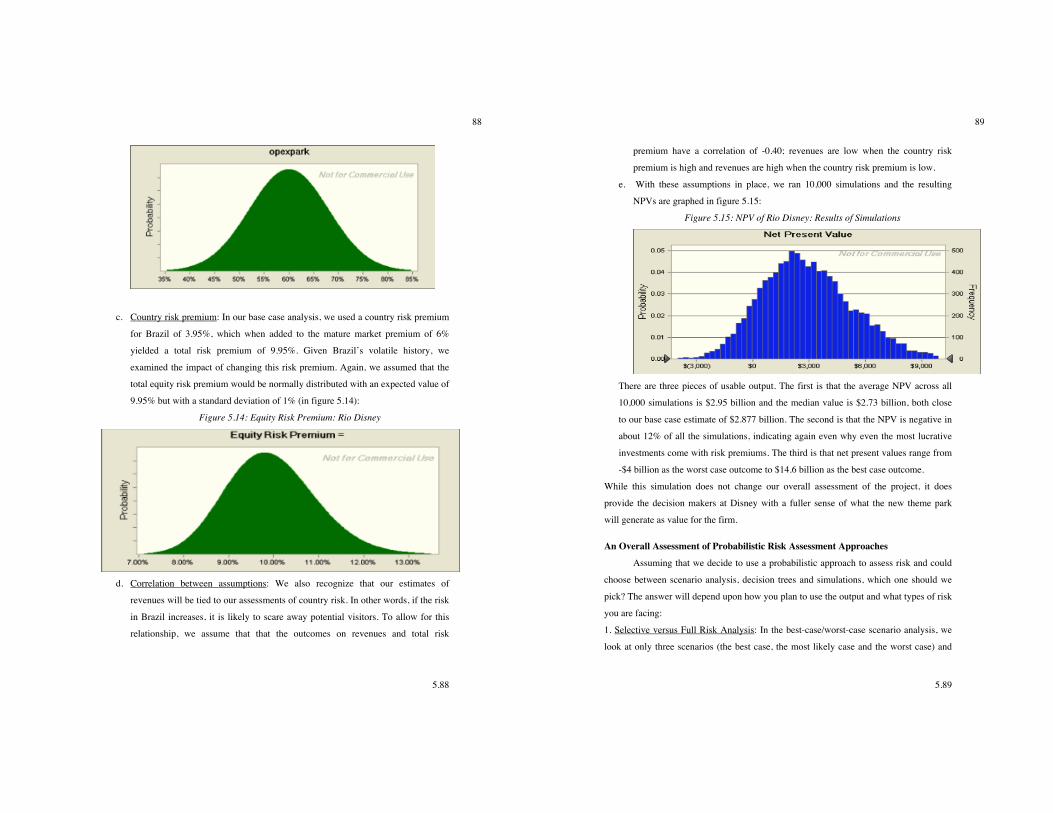
5.88

88

c. Country risk premium: In our base case analysis, we used a country risk premium

for Brazil of 3.95%, which when added to the mature market premium of 6%

yielded a total risk premium of 9.95%. Given Brazil’s volatile history, we

examined the impact of changing this risk premium. Again, we assumed that the

total equity risk premium would be normally distributed with an expected value of

9.95% but with a standard deviation of 1% (in figure 5.14):

Figure 5.14: Equity Risk Premium: Rio Disney

d. Correlation between assumptions: We also recognize that our estimates of

revenues will be tied to our assessments of country risk. In other words, if the risk

in Brazil increases, it is likely to scare away potential visitors. To allow for this

relationship, we assume that that the outcomes on revenues and total risk

5.89

89

premium have a correlation of -0.40; revenues are low when the country risk

premium is high and revenues are high when the country risk premium is low.

e. With these assumptions in place, we ran 10,000 simulations and the resulting

NPVs are graphed in figure 5.15:

Figure 5.15: NPV of Rio Disney: Results of Simulations

There are three pieces of usable output. The first is that the average NPV across all

10,000 simulations is $2.95 billion and the median value is $2.73 billion, both close

to our base case estimate of $2.877 billion. The second is that the NPV is negative in

about 12% of all the simulations, indicating again even why even the most lucrative

investments come with risk premiums. The third is that net present values range from

-$4 billion as the worst case outcome to $14.6 billion as the best case outcome.

While this simulation does not change our overall assessment of the project, it does

provide the decision makers at Disney with a fuller sense of what the new theme park

will generate as value for the firm.

An Overall Assessment of Probabilistic Risk Assessment Approaches Assuming that we decide to use a probabilistic approach to assess risk and could

choose between scenario analysis, decision trees and simulations, which one should we

pick? The answer will depend upon how you plan to use the output and what types of risk

you are facing:

1. Selective versus Full Risk Analysis: In the best-case/worst-case scenario analysis, we

look at only three scenarios (the best case, the most likely case and the worst case) and

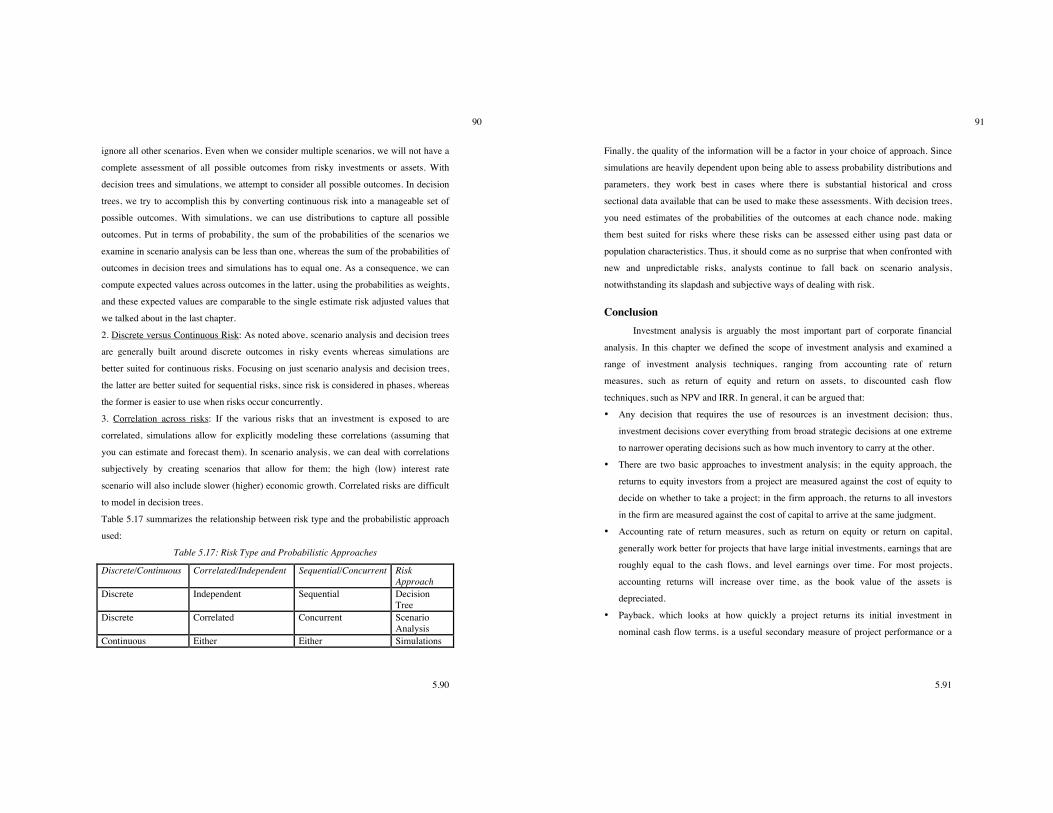
5.90

90

ignore all other scenarios. Even when we consider multiple scenarios, we will not have a

complete assessment of all possible outcomes from risky investments or assets. With

decision trees and simulations, we attempt to consider all possible outcomes. In decision

trees, we try to accomplish this by converting continuous risk into a manageable set of

possible outcomes. With simulations, we can use distributions to capture all possible

outcomes. Put in terms of probability, the sum of the probabilities of the scenarios we

examine in scenario analysis can be less than one, whereas the sum of the probabilities of

outcomes in decision trees and simulations has to equal one. As a consequence, we can

compute expected values across outcomes in the latter, using the probabilities as weights,

and these expected values are comparable to the single estimate risk adjusted values that

we talked about in the last chapter.

2. Discrete versus Continuous Risk: As noted above, scenario analysis and decision trees

are generally built around discrete outcomes in risky events whereas simulations are

better suited for continuous risks. Focusing on just scenario analysis and decision trees,

the latter are better suited for sequential risks, since risk is considered in phases, whereas

the former is easier to use when risks occur concurrently.

3. Correlation across risks: If the various risks that an investment is exposed to are

correlated, simulations allow for explicitly modeling these correlations (assuming that

you can estimate and forecast them). In scenario analysis, we can deal with correlations

subjectively by creating scenarios that allow for them; the high (low) interest rate

scenario will also include slower (higher) economic growth. Correlated risks are difficult

to model in decision trees.

Table 5.17 summarizes the relationship between risk type and the probabilistic approach

used:

Table 5.17: Risk Type and Probabilistic Approaches

Discrete/Continuous Correlated/Independent Sequential/Concurrent Risk Approach

Discrete Independent Sequential Decision Tree

Discrete Correlated Concurrent Scenario Analysis

Continuous Either Either Simulations

5.91

91

Finally, the quality of the information will be a factor in your choice of approach. Since

simulations are heavily dependent upon being able to assess probability distributions and

parameters, they work best in cases where there is substantial historical and cross

sectional data available that can be used to make these assessments. With decision trees,

you need estimates of the probabilities of the outcomes at each chance node, making

them best suited for risks where these risks can be assessed either using past data or

population characteristics. Thus, it should come as no surprise that when confronted with

new and unpredictable risks, analysts continue to fall back on scenario analysis,

notwithstanding its slapdash and subjective ways of dealing with risk.

Conclusion Investment analysis is arguably the most important part of corporate financial

analysis. In this chapter we defined the scope of investment analysis and examined a

range of investment analysis techniques, ranging from accounting rate of return

measures, such as return of equity and return on assets, to discounted cash flow

techniques, such as NPV and IRR. In general, it can be argued that:

• Any decision that requires the use of resources is an investment decision; thus,

investment decisions cover everything from broad strategic decisions at one extreme

to narrower operating decisions such as how much inventory to carry at the other.

• There are two basic approaches to investment analysis; in the equity approach, the

returns to equity investors from a project are measured against the cost of equity to

decide on whether to take a project; in the firm approach, the returns to all investors

in the firm are measured against the cost of capital to arrive at the same judgment.

• Accounting rate of return measures, such as return on equity or return on capital,

generally work better for projects that have large initial investments, earnings that are

roughly equal to the cash flows, and level earnings over time. For most projects,

accounting returns will increase over time, as the book value of the assets is

depreciated.

• Payback, which looks at how quickly a project returns its initial investment in

nominal cash flow terms, is a useful secondary measure of project performance or a

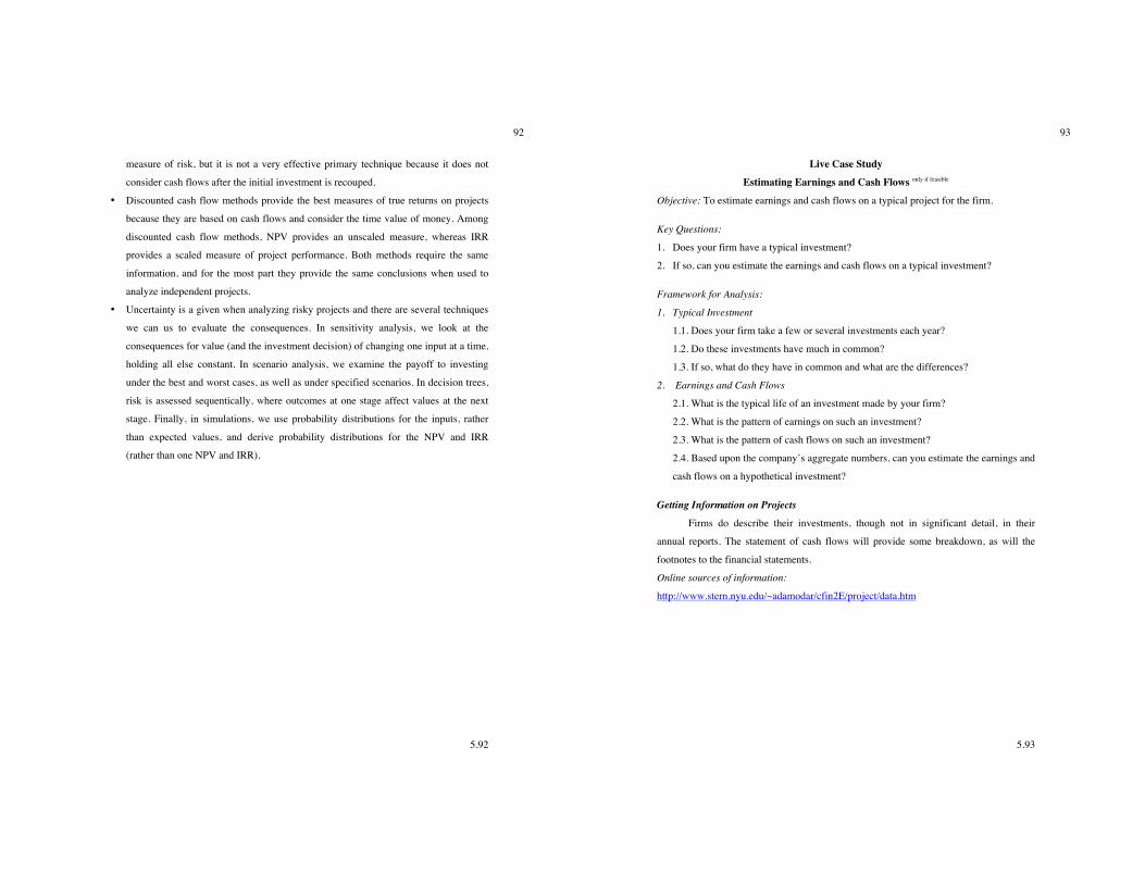
5.92

92

measure of risk, but it is not a very effective primary technique because it does not

consider cash flows after the initial investment is recouped.

• Discounted cash flow methods provide the best measures of true returns on projects

because they are based on cash flows and consider the time value of money. Among

discounted cash flow methods, NPV provides an unscaled measure, whereas IRR

provides a scaled measure of project performance. Both methods require the same

information, and for the most part they provide the same conclusions when used to

analyze independent projects.

• Uncertainty is a given when analyzing risky projects and there are several techniques

we can us to evaluate the consequences. In sensitivity analysis, we look at the

consequences for value (and the investment decision) of changing one input at a time,

holding all else constant. In scenario analysis, we examine the payoff to investing

under the best and worst cases, as well as under specified scenarios. In decision trees,

risk is assessed sequentically, where outcomes at one stage affect values at the next

stage. Finally, in simulations, we use probability distributions for the inputs, rather

than expected values, and derive probability distributions for the NPV and IRR

(rather than one NPV and IRR).

5.93

93

Live Case Study Estimating Earnings and Cash Flows only if feasible

Objective: To estimate earnings and cash flows on a typical project for the firm.

Key Questions:

1. Does your firm have a typical investment?

2. If so, can you estimate the earnings and cash flows on a typical investment?

Framework for Analysis:

1. Typical Investment

1.1. Does your firm take a few or several investments each year?

1.2. Do these investments have much in common?

1.3. If so, what do they have in common and what are the differences?

2. Earnings and Cash Flows

2.1. What is the typical life of an investment made by your firm?

2.2. What is the pattern of earnings on such an investment?

2.3. What is the pattern of cash flows on such an investment?

2.4. Based upon the company’s aggregate numbers, can you estimate the earnings and

cash flows on a hypothetical investment?

Getting Information on Projects

Firms do describe their investments, though not in significant detail, in their

annual reports. The statement of cash flows will provide some breakdown, as will the

footnotes to the financial statements.

Online sources of information:

http://www.stern.nyu.edu/~adamodar/cfin2E/project/data.htm

5.94

94

Problems and Questions 1. You have been given the following information on a project:

• It has a five-year lifetime

• The initial investment in the project will be $25 million, and the investment will be

depreciated straight line, down to a salvage value of $10 million at the end of the fifth

year.

• The revenues are expected to be $20 million next year and to grow 10% a year after

that for the remaining four years.

• The cost of goods sold, excluding depreciation, is expected to be 50% of revenues.

• The tax rate is 40%.

a. Estimate the pretax return on capital, by year and on average, for the project.

b. Estimate the after-tax return on capital, by year and on average, for the project.

c. If the firm faced a cost of capital of 12%, should it take this project?

2. Now assume that the facts in Problem 1 remain unchanged except for the depreciation

method, which is switched to an accelerated method with the following depreciation

schedule:

Year % of Depreciable Asset

1 40%

2 20%

3 14.4%

4 13.3%

5 13.3%

Depreciable Asset = Initial Investment – Salvage Value

a. Estimate the pretax return on capital, by year and on average, for the project.

b. Estimate the after-tax return on capital, by year and on average, for the project.

c. If the firm faced a cost of capital of 12%, should it take this project?

3. Consider again the project described in Problem 1 (assume that the depreciation reverts

to a straight line). Assume that 40% of the initial investment for the project will be

financed with debt, with an annual interest rate of 10% and a balloon payment of the

principal at the end of the fifth year.

5.95

95

a. Estimate the return on equity, by year and on average, for this project.

b. If the cost of equity is 15%, should the firm take this project?

4. Answer true or false to the following statements:

a. The return on equity for a project will always be higher than the return on capital on

the same project.

b. If the return on capital is less than the cost of equity, the project should be rejected.

c. Projects with high financial leverage will have higher interest expenses and lower net

income than projects with low financial leverage and thus end up with a lower return on

equity.

d. Increasing the depreciation on an asset will increase the estimated return on capital and

equity on the project.

e. The average return on equity on a project over its lifetime will increase if we switch

from straight line to double declining balance depreciation.

5. Under what conditions will the return on equity on a project be equal to the IRR,

estimated from cash flows to equity investors, on the same project?

6. You are provided with the projected income statements for a project:

Year 1 2 3 4

Revenues ($) $10,000 $11,000 $12,000 $13,000

– Cost of goods sold ($) $4,000 $4,400 $4,800 $5,200

– Depreciation $4,000 $3,000 $2,000 $1,000

= EBIT $2,000 $3,600 $5,200 $6,800

• The tax rate is 40%.

• The project required an initial investment of $15,000 and an additional investment of

$2,000 at the end of year two.

• The working capital is anticipated to be 10% of revenues, and the working capital

investment has to be made at the beginning of each period.

a. Estimate the free cash flow to the firm for each of the four years.

b. Estimate the payback period for investors in the firm.

c. Estimate the NPV to investors in the firm, if the cost of capital is 12%. Would you

accept the project?

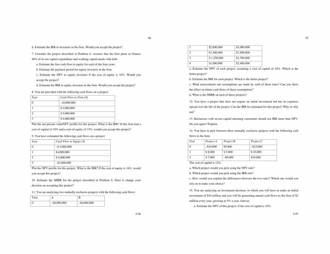
5.96

96

d. Estimate the IRR to investors in the firm. Would you accept the project?

7. Consider the project described in Problem 6. Assume that the firm plans to finance

40% of its net capital expenditure and working capital needs with debt.

a. Estimate the free cash flow to equity for each of the four years.

b. Estimate the payback period for equity investors in the firm.

c. Estimate the NPV to equity investors if the cost of equity is 16%. Would you

accept the project?

d. Estimate the IRR to equity investors in the firm. Would you accept the project?

8. You are provided with the following cash flows on a project:

Year Cash Flow to Firm ($)

0 –10,000,000

1 $ 4,000,000

2 $ 5,000,000

3 $ 6,000,000

Plot the net present valueNPV profile for this project. What is the IRR? If this firm had a

cost of capital of 10% and a cost of equity of 15%, would you accept this project?

9. You have estimated the following cash flows on a project:

Year Cash Flow to Equity ($)

0 –$ 5,000,000

1 $4,000,000

2 $ 4,000,000

3 –$3,000,000

Plot the NPV profile for this project. What is the IRR? If the cost of equity is 16%, would

you accept this project?

10. Estimate the MIRR for the project described in Problem 8. Does it change your

decision on accepting this project?

11. You are analyzing two mutually exclusive projects with the following cash flows:

Year A B

0 –$4,000,000 –$4,000,000

5.97

97

1 $2,000,000 $1,000,000

2 $1,500,000 $1,500,000

3 $ 1,250,000 $1,700,000

4 $1,000,000 $2,400,000

a. Estimate the NPV of each project, assuming a cost of capital of 10%. Which is the

better project?

b. Estimate the IRR for each project. Which is the better project?

c. What reinvestment rate assumptions are made by each of these rules? Can you show

the effect on future cash flows of these assumptions?

d. What is the MIRR on each of these projects?

12. You have a project that does not require an initial investment but has its expenses

spread over the life of the project. Can the IRR be estimated for this project? Why or why

not?

13. Businesses with severe capital rationing constraints should use IRR more than NPV.

Do you agree? Explain.

14. You have to pick between three mutually exclusive projects with the following cash

flows to the firm:

Year Project A Project B Project C

0 –$10,000 $5,000 –$15,000

1 $ 8,000 $ 5,000 $ 10,000

2 $ 7,000 –$8,000 $10,000

The cost of capital is 12%.

a. Which project would you pick using the NPV rule?

b. Which project would you pick using the IRR rule?

c. How would you explain the differences between the two rules? Which one would you

rely on to make your choice?

15. You are analyzing an investment decision, in which you will have to make an initial

investment of $10 million and you will be generating annual cash flows to the firm of $2

million every year, growing at 5% a year, forever.

a. Estimate the NPV of this project, if the cost of capital is 10%.

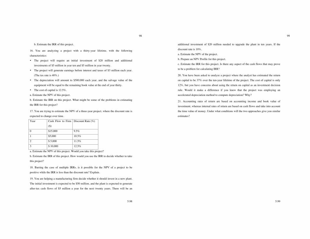
5.98

98

b. Estimate the IRR of this project.

16. You are analyzing a project with a thirty-year lifetime, with the following

characteristics:

• The project will require an initial investment of $20 million and additional

investments of $5 million in year ten and $5 million in year twenty.

• The project will generate earnings before interest and taxes of $3 million each year.

(The tax rate is 40%.)

• The depreciation will amount to $500,000 each year, and the salvage value of the

equipment will be equal to the remaining book value at the end of year thirty.

• The cost of capital is 12.5%.

a. Estimate the NPV of this project.

b. Estimate the IRR on this project. What might be some of the problems in estimating

the IRR for this project?

17. You are trying to estimate the NPV of a three-year project, where the discount rate is

expected to change over time.

Year Cash Flow to Firm

($)

Discount Rate (%)

0 $15,000 9.5%

1 $5,000 10.5%

2 $ 5,000 11.5%

3 $ 10,000 12.5%

a. Estimate the NPV of this project. Would you take this project?

b. Estimate the IRR of this project. How would you use the IRR to decide whether to take

this project?

18. Barring the case of multiple IRRs, is it possible for the NPV of a project to be

positive while the IRR is less than the discount rate? Explain.

19. You are helping a manufacturing firm decide whether it should invest in a new plant.

The initial investment is expected to be $50 million, and the plant is expected to generate

after-tax cash flows of $5 million a year for the next twenty years. There will be an

5.99

99

additional investment of $20 million needed to upgrade the plant in ten years. If the

discount rate is 10%,

a. Estimate the NPV of the project.

b. Prepare an NPV Profile for this project.

c. Estimate the IRR for this project. Is there any aspect of the cash flows that may prove

to be a problem for calculating IRR?

20. You have been asked to analyze a project where the analyst has estimated the return

on capital to be 37% over the ten-year lifetime of the project. The cost of capital is only

12%, but you have concerns about using the return on capital as an investment decision

rule. Would it make a difference if you knew that the project was employing an

accelerated depreciation method to compute depreciation? Why?

21. Accounting rates of return are based on accounting income and book value of

investment, whereas internal rates of return are based on cash flows and take into account

the time value of money. Under what conditions will the two approaches give you similar

estimates?