People around the world are wearing masksto protect themselves against swine flu. (Source: http://www.baltimoresun.com/news/nation-world/ny-swineflu-photos,0,859331.photogallery [Getty Images Photo / May 2, 2009].)

13Wildlife, Fisheries, and Endangered Species

L E A R N I N G O B J E C T I V E S

Wildlife, fish, and endangered species are among the

most popular environmental issues today. People

love to see wildlife; many people enjoy fishing, make

a living from it, or rely on fish as an important part

of their diet; and since the 19th century the fate of

endangered species has drawn public attention. You

would think that by now we would be doing a good

job of conserving and managing these kinds of life,

but often we are not. This chapter tells you how we

are doing and how we can improve our conservation

and management of wildlife, fisheries, and endan-

gered species. After reading this chapter, you should

understand . . .

Why people want to conserve wildlife and endan-

gered species;

The importance of habitat, ecosystems, and land-

scape in the conservation of endangered species;

Current causes of extinction;

Steps we can take to achieve sustainability of wildlife,

fisheries, and endangered species;

The concepts of species persistence, maximum

sustainable yield, the logistic growth curve, carrying

capacity, optimum sustainable yield, and minimum

viable populations.

CH

AP

TE

R

Brown pelicans, once endangered because of DDT, have come back in abundance and are common along both the Atlantic and Pacific coasts. This pelican is fishing from a breakwater on the Atlantic coast of Florida.

258 C H A P T E R 1 3 Wildlife, Fisheries, and Endangered Species

C A S E S T U D Y

The grizzly bear and the American bison illustrate many of the general problems of conserving and managing wildlife and endangered species. In Chapter 2 we pointed out that the standard scientific method sometimes does not seem suited to studies in the environmental sciences. This is also true of some aspects of wildlife management and conservation. Several examples illustrate the needs and problems.

The Grizzly Bear

A classic example of wildlife management is the North American grizzly bear. An endangered species, the grizzly has been the subject of efforts by the U.S. Fish and Wild-life Service to meet the requirements of the U.S. Endan-gered Species Act, which include restoring the population of these bears.

The grizzly became endangered as a result of hunting and habitat destruction. It is arguably the most danger-ous North American mammal, famous for unprovoked attacks on people, and has been eliminated from much of its range for that reason. Males weigh as much as 270 kg (600 pounds), females as much as 160 kg (350 pounds). When they rear up on their hind legs, they are almost 3 m (8 ft) tall. No wonder they are frightening (see Figure 13.1). Despite this, or perhaps because of it, grizzlies intrigue people, and watching grizzlies from a safe distance has become a popular recreation.

At first glance, restoring the grizzly seems simple enough. But then that old question arises: Restore to

what? One answer is to restore the species to its abundance at the time of the European discovery and settlement of North America. But it turns out that there is very little historical information about the abundance of the griz-zly at that time, so it is not easy to determine how many (or what density per unit area) could be considered a “re-stored” population. We also lack a good estimate of the grizzly’s present abundance, and thus we don’t know how far we will have to take the species to “restore” it to some hypothetical past abundance. Moreover, the grizzly is dif-ficult to study—it is large and dangerous and tends to be reclusive. The U.S. Fish and Wildlife Service attempted to count the grizzlies in Yellowstone National Park by in-stalling automatic flash cameras that were set off when the grizzlies took a bait. This seemed a good idea, but the griz-zlies didn’t like the cameras and destroyed them,1 so we still don’t have a good scientific estimate of their present number. The National Wildlife Federation lists 1,200 in the contiguous states, 32,000 in Alaska, and about 25,000 in Canada, but these are crude estimates.2

How do we arrive at an estimate of a population that existed at a time when nobody thought of counting its members? Where possible, we use historical records, as dis-cussed in Chapter 2. We can obtain a crude estimate of the grizzly’s abundance at the beginning of the 19th cen-tury from the journals of the Lewis and Clark expedition. Lewis and Clark did not list the numbers of most wildlife they saw; they simply wrote that they saw “many” bison, elk, and so forth. But the grizzlies were especially danger-ous and tended to travel alone, so Lewis and Clark noted each encounter, stating the exact number they met. On that expedition, they saw 37 grizzly bears over a distance of ap-proximately 1,000 miles (their records were in miles).1

Lewis and Clark saw grizzlies from near what is now Pierre, South Dakota, to what is today Missoula, Montana. A northern and southern geographic limit to the grizzly’s range can be obtained from other explorers. Assuming Lewis and Clark could see a half-mile to each side of their line of travel on average, the density of the bears was ap-proximately 3.7 per 100 square miles. If we estimate that the bears’ geographic range was 320,000 square miles in the mountain and western plains states, we arrive at a total population of 320,000 x 0.37, or about 12,000 bears.

Suppose we phrase this as a hypothesis: “The number of grizzly bears in 1805 in what is now the United States was 12,000.” Is this open to disproof? Not without time

Stories Told by the Grizzly Bear and the Bison

FIGURE 13.1 Grizzly bear. Records of bear sightings by Lewis and Clark have been used to estimate their population at the begin-ning of the 19th century.

Case Study: Stories Told by the Grizzly Bear and the Bison 259

travel. Therefore, it is not a scientific statement; it can only be taken as an educated guess or, more formally, an assumption or premise. Still, it has some basis in histori-cal documents, and it is better than no information, since we have few alternatives to determine what used to be. We can use this assumption to create a plan to restore the grizzly to that abundance. But is this the best approach?

Another approach is to ask what is the minimum viable population of grizzly bears—forget completely about what might have been the situation in the past and make use of modern knowledge of population dynamics and genet-ics, along with food requirements and potential production of that food. Studies of existing populations of brown and grizzly bears suggest that only populations larger than 450 individuals respond to protection with rapid growth.2 Us-ing this approach, we could estimate how many bears ap-pear to be a “safe” number—that is, a number that carries small risk of extinction and loss of genetic diversity. More precisely, we could phrase this statement as “How many bears are necessary so that the probability that the grizzly will become extinct in the next ten years [or some other period that we consider reasonable for planning] is less than 1% [or some other percentage that we would like]?”

With appropriate studies, this approach could have a scientific basis. Consider a statement of this kind phrased as a hypothesis: “A population of 450 bears [or some other number] results in a 99% chance that at least one ma-ture male and one mature female will be alive ten years from today.” We can disprove this statement, but only by waiting for ten years to go by. Although it is a scientific statement, it is a difficult one to deal with in planning for the present.

The American Bison

Another classic case of wildlife management, or mis-management, is the demise of the American bison, or buffalo (Figure 13.2a). The bison was brought close to extinction in the 19th century for two reasons: They were hunted because coats made of bison hides had become fashionable in Europe, and they also were killed as part of warfare against the Plains peoples (Figure 13.2b). U.S. Army Colonel R.I. Dodge was quoted in 1867 as saying, “Kill every buffalo you can. Every buffalo dead is an Indian gone.”1

Unlike the grizzly bear, the bison has recovered, in large part because ranchers have begun to find them profitable to raise and sell for meat and other products. Informal estimates, including herds on private and public ranges, suggest there are 200,000–300,000, and bison are said to occur in every state in the United States, including Hawaii, a habitat quite different from their original Great Plains home range.3 About 20,000 roam wild on public lands in the United States and Canada.4

How many bison were there before European set-tlement of the American West? And how low did their numbers drop? Historical records provide insight. In 1865 the U.S. Army, in response to Indian attacks in the fall of 1864, set fires to drive away the Indi-ans and the buffalo, killing vast numbers of animals.5

The speed with which bison were almost eliminated was surprising—even to many of those involved in hunting them.

Many early writers tell of immense herds of bison, but few counted them. One exception was General Isaac I. Stevens, who, on July 10, 1853, was surveying for the transcontinental railway in North Dakota. He and his men climbed a high hill and saw “for a great dis-tance ahead every square mile” having “a herd of buffalo upon it.” He wrote that “their number was variously estimated by the members of the party—some as high as half a million. I do not think it any exaggeration to

FIGURE 13.2 (a) A bison ranch in the United States. In recent years, interest in growing bison ranches has increased greatly. In part, the goal is to restore bison to a reasonable percentage of its numbers before the Civil War. In part, bison are ranched because people like them. In addition, there is a growing market for bison meat and other products, including cloth made from bison hair. (b) Painting of a buffalo hunt by George Catlin in 1832–1833 at the mouth of the Yellowstone River.

(a)

(b)

260 C H A P T E R 1 3 Wildlife, Fisheries, and Endangered Species

set it down at 200,000.”1 In short, his estimate of just one herd was about the same number of bison that exist in total today!

One of the better attempts to estimate the number of buffalo in a herd was made by Colonel R. I. Dodge, who took a wagon from Fort Zarah to Fort Larned on the Ar-kansas River in May 1871, a distance of 34 miles. For at least 25 of those miles, he found himself in a “dark blan-ket” of buffalo. He estimated that the mass of animals he saw in one day totaled 480,000. At one point, he and his men traveled to the top of a hill from which he estimated that he could see six to ten miles, and from that high point there appeared to be a single solid mass of buffalo extending over 25 miles. At ten animals per acre, not a particularly high density, the herd would have numbered 2.7–8.0 million animals.1

In the fall of 1868, “a train traveled 120 miles be-tween Ellsworth and Sheridan, Wyoming, through a continuous, browsing herd, packed so thick that the en-gineer had to stop several times, mostly because the buf-faloes would scarcely get off the tracks for the whistle and the belching smoke.”5 That spring, a train had been de-layed for eight hours while a single herd passed “in one steady, unending stream.” We can use accounts like this one to set bounds on the possible number of animals seen. At the highest extreme, we can assume that the train bi-sected a circular herd with a diameter of 120 miles. Such a herd would cover 11,310 square miles, or more than 7 million acres. If we suppose that people exaggerated the density of the buffalo, and there were only ten per acre, this single herd would still have numbered 70 million animals!

Some might say that this estimate is probably too high, because the herd would more likely have formed a broad, meandering, migrating line rather than a cir-cle. The impression remains the same—there were huge numbers of buffalo in the American West even as late as 1868, numbering in the tens of millions and probably

50 million or more. Ominously, that same year, the Kan-sas Pacific Railroad advertised a “Grand Railway Excur-sion and Buffalo Hunt.”5 Some say that many hunters believed the buffalo could never be brought to extinction because there were so many. The same was commonly be-lieved about all of America’s living resources throughout the 19th century.

We tend to view environmentalism as a social and political movement of the 20th century, but it is said that after the Civil War there were angry protests in ev-ery legislature over the slaughter of buffalo. In 1871 the U.S. Biological Survey sent George Grinnell to survey the herds along the Platte River. He estimated that only 500,000 buffalo remained there and that at the then-current rate of killing, the animals would not last long. As late as the spring of 1883, a herd of an estimated 75,000 crossed the Yellowstone River near Miles City, Montana, but fewer than 5,000 reached the Canadian border.5 By the end of that year—only 15 years after the Kansas Pacific train was delayed for eight hours by a huge herd of buffalo—only a thousand or so buffalo could be found, 256 in captivity and about 835 roaming the plains. A short time later, there were only 50 buffalo wild on the plains.

Today, more and more ranchers are finding ways to maintain bison, and the market for bison meat and other bison products is growing, along with an increas-ing interest in reestablishing bison herds for aesthetic, spiritual, and moral reasons. The history of the bison once again raises the question of what we mean by “re-store” a population. Even with our crude estimates of original abundances, the numbers would have varied from year to year. So we would have to “restore” bison not to a single number independent of the ability of its habitat to support the population, but to some range of abundances. How do we approach that problem and estimate the range?

13.1 Traditional Single-Species Wildlife ManagementWildlife, fisheries, and endangered species are considered together in this chapter because they have a common history of exploitation, management, and conservation, and because modern attempts to manage and conserve them follow the same approaches. Although any form of life, from bacteria and fungi to flowering plants and ani-mals, can become endangered, concern about endangered species has tended to focus on wildlife. We will maintain

that focus, but we ask you to remember that the general principles apply to all forms of life.

Attempts to apply science to the conservation and management of wildlife and fisheries, and therefore to endangered species, began around the turn of the 20th century and viewed each species as a single population in isolation.

Carrying Capacity and Sustainable Yields

The classical, early-20th-century idea of wildlife and fisheries was formalized in the S-shaped logistic growth curve (Figure 13.3), which we discussed in Chapter 4.

1 3 . 1 Traditional Single-Species Wildlife Management 261

As explained in that chapter, the logistic growth curve assumes that changes in the size of a population are simply the result of the population’s size in relation to a maximum, called the carrying capacity. The logistic characterizes the population only by its total size, noth-ing else—not the ratio of young to old, healthy to sick, males to females, and the environment doesn’t appear at all; it is just assumed to be constant. (See the accompa-nying box Key Characteristics of a Logistic Population.) The carrying capacity is defined simply as the maximum population that can be sustained indefinitely. Implicit in this definition is the idea that if the population exceeds the carrying capacity, it will damage its environment and/or its own ability to grow and reproduce, and therefore the population will decline.

Two management goals resulted from these ideas and the logistic equation: For a species that we intend to harvest, the goal was maximum sustainable yield (MSY); for a species that we wish to conserve, the goal was to have that species reach, and remain at, its carrying capacity. Maximum sus-tainable yield is defined as the maximum growth rate (mea-sured either as a net increase in the number of individuals or in biomass over a specified time period) that the population could sustain indefinitely. The maximum sustainable-yield population is defined as the population size at which the maximum growth rate occurs. More simply, the population was viewed as a factory that could keep churning out exactly the same quantity of a product year after year.

Today a broader view is developing. It acknowledges that a population exists within an ecological community and within an ecosystem, and that the environment is always, or almost always, changing (including human-induced changes). Therefore, the population you are in-terested in interacts with many others, and the size and condition of those can affect the one on which you are focusing. With this new understanding, the harvesting goal is to harvest sustainably, removing in each time pe-riod the maximum number of individuals (or maximum biomass) that can be harvested indefinitely without di-minishing either the population that particularly inter-ests you or its ecosystem. The preservation goal for a threatened or an endangered species becomes more open, with more choices. One is to try to keep the population at its carrying capacity. Another is to sustain a minimum viable population, which is the estimated smallest popu-lation that can maintain itself and its genetic variability indefinitely. A third option, which leads to a population size somewhere between the other two, is the optimum sustainable population.

In the logistic curve, the greatest production occurs when the population is exactly one-half of the carrying capacity (see Figure 13.3). This is nifty because it makes everything seem simple—all you have to do is figure out the carrying capacity and keep the population at one-half of it. But what seems simple can easily become trouble-some. Even if the basic assumptions of the logistic curve were true, which they are not, the slightest overestimate of carrying capacity, and therefore MSY, would lead to over-harvesting, a decline in production, and a decline in the abundance of the species. If a population is harvested as if it were actually at one-half its carrying capacity, then un-less a logistic population is actually maintained at exactly that number, its growth will decline. Since it is almost impossible to maintain a wild population at some exact number, the approach is doomed from the start.

One important result of all of this is that a logistic popu-lation is stable in terms of its carrying capacity—it will return to that number after a disturbance. If the population grows beyond its carrying capacity, deaths exceed births, and the population declines back to the carrying capacity. If the population falls below the carrying capacity, births exceed deaths, and the population increases. Only if the popula-tion is exactly at the carrying capacity do births exactly equal deaths, and then the population does not change.

Despite its limitations, the logistic growth curve was used for all wildlife, especially fisheries and including en-dangered species, throughout much of the 20th century.

The term carrying capacity as used today has three definitions. The first is the carrying capacity as defined by the logistic growth curve, the logistic carrying capacity already discussed. The second definition contains the same idea but is not dependent on that specific equation. It states that the

Key Characteristics of a Logistic Population

The population exists in an environment assumed to be constant.

The population is small in relation to its resources and therefore grows at a nearly exponential rate.

Competition among individuals in the population slows the growth rate.

The greater the number of individuals, the greater the competition and the slower the rate of growth.

Eventually, a point is reached, called the logistic car-rying capacity, at which the number of individuals is just sufficient for the available resources.

At this level, the number of births in a unit time equals the number of deaths, and the population is constant.

A population can be described simply by its total number.

Therefore, all individuals are equal.

262 C H A P T E R 1 3 Wildlife, Fisheries, and Endangered Species

carrying capacity is an abundance at which a population can sustain itself without any detrimental effects that would lessen the ability of that species—in the abstract, treated as separated from all others—to maintain that abundance. The third, the optimum sustainable population, already discussed, leads to a population size between the other two.

An Example of Problems with the Logistic Curve

Suppose you are in charge of managing a deer herd for recreational hunting in one of the 50 U.S. states. Your goal is to maintain the population at its MSY level,

which, as you can see from Figure 13.3, occurs at exactly one-half of the carrying capacity. At this abundance, the population increases by the greatest number during any time period.

To accomplish this goal, first you have to determine the logistic carrying capacity. You are immediately in trouble because, first, only in a few cases has the carry-ing capacity ever been determined by legitimate scientific methods (see Chapter 2) and, second, we now know that the carrying capacity varies with changes in the environ-ment. The procedure in the past was to estimate the car-rying capacity by nonscientific means and then attempt to maintain the population at one-half that level. This method requires accurate counts each year. It also requires

Logi

stic

cur

ve

0 20 40 60 80 1000

20

10

40

30

50

60

80

70

90

100

120 140 160Time

Pop

ulat

ion

size

(th

ousa

nds)

No harvest MSY overharvest MSY correct

Population estimated correctly

Population overestimated

MSYpopulation

size

Carrying capacity

(a)

Sur

plus

of r

ecru

itmen

t ove

r lo

ss(p

oten

tial s

usta

inab

le h

arve

st)

MSY level

Population size

Original level, orcarrying capacity

Maximumsustainable

yield

(b)

FIGURE 13.3 (a) The logistic growth curve, showing the carrying capacity and the maximum sustainable yield (MSY) population (where the population size is one-half the carrying capacity). The figure shows what happens to a population when we assume it is at MSY and it is not. Sup-pose a population grows according to the logistic curve from a small number to a carrying capac-ity of 100,000 with an annual growth rate of 5%. The correct maximum sustainable yield would be 50,000. When the population reaches exactly the calculated maximum sustainable yield, the popu-lation continues to be constant. But if we make a mistake in estimating the size of the population (for example, if we believe that it is 60,000 when it is only 50,000), then the harvest will always be too large, and we will drive the population to extinction. (b) Another view of a logistic popu-lation. Growth in the population here is graphed against population size. Growth peaks when the population is exactly at one-half the carrying capacity. This is a mathematical consequence of the equation for the curve. It is rarely, if ever, observed in nature.

1 3 . 2 Improved Approaches to Wildlife Management 263

that the environment not vary, or, if it does, that it vary in a way that does not affect the population. Since these conditions cannot be met, the logistic curve has to fail as a basis for managing the deer herd.

An interesting example of the staying power of the lo-gistic growth curve can be found in the United States Ma-rine Mammal Protection Act of 1972. This act states that its primary goal is to conserve “the health and stability of marine ecosystems,” which is part of the modern approach, and so the act seems to be off to a good start. But then the act states that the secondary goal is to maintain an “opti-mum sustainable population” of marine mammals. What is this? The wording of the act allows two interpretations. One is the logistic carrying capacity, and the other is the MSY population level of the logistic growth curve. So the act takes us back to square one, the logistic curve.

13.2 Improved Approaches to Wildlife Management The U.S. Council on Environmental Quality (an office within the executive branch of the federal government), the World Wildlife Fund of the United States, the Ecological Society of America, the Smithsonian Institution, and the In-ternational Union for the Conservation of Nature (IUCN) have proposed four principles of wildlife conservation:

A safety factor in terms of population size, to allow for limitations of knowledge and imperfections of proce-dures. An interest in harvesting a population should not allow the population to be depleted to some theoretical minimum size.

Concern with the entire community of organisms and all the renewable resources, so that policies developed for one species are not wasteful of other resources.

Maintenance of the ecosystem of which the wildlife are a part, minimizing risk of irreversible change and long-term adverse effects as a result of use.

Continual monitoring, analysis, and assessment. The application of science and the pursuit of knowledge about the wildlife of interest and its ecosystem should be maintained and the results made available to the public.

These principles broaden the scope of wildlife man-agement from a narrow focus on a single species to inclu-sion of the ecological community and ecosystem. They call for a safety net in terms of population size, meaning that no population should be held at exactly the MSY level or reduced to some theoretical minimum abundance. These new principles provide a starting point for an improved approach to wildlife management.

Time Series and Historical Range of Variation

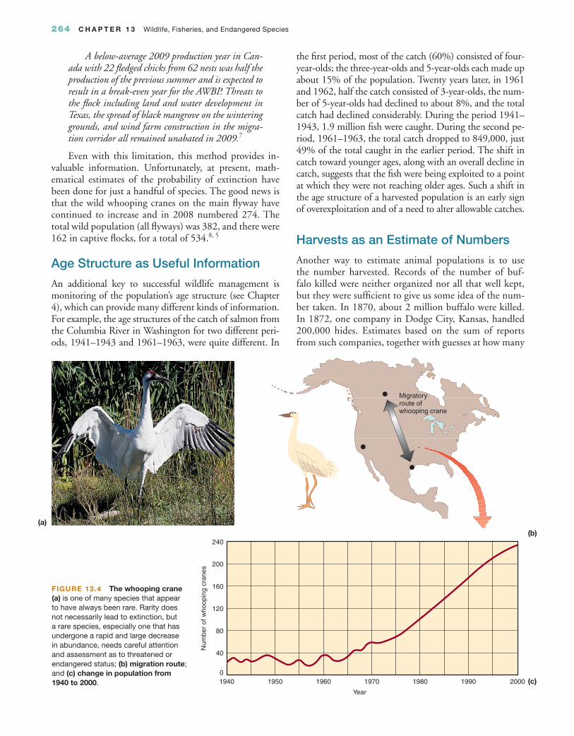
As illustrated by the opening case study about the Ameri-can buffalo and grizzly bears, it is best to have an estimate of population over a number of years. This set of esti-mates is called a time series and could provide us with a measure of the historical range of variation—the known range of abundances of a population or species over some past time interval. Such records exist for few species. One is the American whooping crane (Figure 13.4), America’s tallest bird, standing about 1.6 m (5 ft) tall. Because this species became so rare and because it migrated as a sin-gle flock, people began counting the total population in the late 1930s. At that time, they saw only 14 whooping cranes. They counted not only the total number but also the number born that year. The difference between these two numbers gives the number dying each year as well. And from this time series, we can estimate the probability of extinction.

The first estimate of the probability of extinction based on the historical range of variation, made in the early 1970s, was a surprise. Although the birds were few, the probability of extinction was less than one in a billion.6 How could this number be so low? Use of the historical range of variation carries with it the assump-tion that causes of variation in the future will be only those that occurred during the historical period. For the whooping cranes, one catastrophe—such as a long, un-precedented drought on the wintering grounds—could cause a population decline not observed in the past.

Not that the whooping crane is without threats—current changes in its environment may not be sim-ply repeats of what happened in the past. According to Tom Stehn, Whooping Crane Coordinator for the U.S. Fish and Wildlife Service, the whooping crane popula-tion that winters in Aransas National Wildlife Refuge, Texas, and summers in Wood Buffalo National Park, Canada,

reached a record population of 270 at Aransas in December, 2008. The number would have been sub-stantially higher but for the loss of 34 birds that left Aransas in the spring, 2008 and failed to return in the fall. Faced with food shortages from an “excep-tional” drought that hammered Texas, record high mortality during the 2008–09 winter of 23 cranes (8.5% of the flock) left the AWBP at 247 in the spring, 2009. Total flock mortality for the 12 months following April, 2008 equaled 57 birds (21.4% of the flock). The refuge provided supplemental feed during the 2008–09 winter to provide some cranes with additional calories. Two whooping cranes failed to migrate north, but survived the hot and dry 2009 Aransas summer.

264 C H A P T E R 1 3 Wildlife, Fisheries, and Endangered Species

A below-average 2009 production year in Can-ada with 22 fledged chicks from 62 nests was half the production of the previous summer and is expected to result in a break-even year for the AWBP. Threats to the flock including land and water development in Texas, the spread of black mangrove on the wintering grounds, and wind farm construction in the migra-tion corridor all remained unabated in 2009.7

Even with this limitation, this method provides in-valuable information. Unfortunately, at present, math-ematical estimates of the probability of extinction have been done for just a handful of species. The good news is that the wild whooping cranes on the main flyway have continued to increase and in 2008 numbered 274. The total wild population (all flyways) was 382, and there were 162 in captive flocks, for a total of 534.8, 5

Age Structure as Useful Information

An additional key to successful wildlife management is monitoring of the population’s age structure (see Chapter 4), which can provide many different kinds of information. For example, the age structures of the catch of salmon from the Columbia River in Washington for two different peri-ods, 1941–1943 and 1961–1963, were quite different. In

the first period, most of the catch (60%) consisted of four-year-olds; the three-year-olds and 5-year-olds each made up about 15% of the population. Twenty years later, in 1961 and 1962, half the catch consisted of 3-year-olds, the num-ber of 5-year-olds had declined to about 8%, and the total catch had declined considerably. During the period 1941–1943, 1.9 million fish were caught. During the second pe-riod, 1961–1963, the total catch dropped to 849,000, just 49% of the total caught in the earlier period. The shift in catch toward younger ages, along with an overall decline in catch, suggests that the fish were being exploited to a point at which they were not reaching older ages. Such a shift in the age structure of a harvested population is an early sign of overexploitation and of a need to alter allowable catches.

Harvests as an Estimate of Numbers

Another way to estimate animal populations is to use the number harvested. Records of the number of buf-falo killed were neither organized nor all that well kept, but they were sufficient to give us some idea of the num-ber taken. In 1870, about 2 million buffalo were killed. In 1872, one company in Dodge City, Kansas, handled 200,000 hides. Estimates based on the sum of reports from such companies, together with guesses at how many

1950 1960 1970 1980 1990

Year

Migratoryroute ofwhooping crane

20000

40

80

120

160

200

240

1940

Num

ber

of w

hoop

ing

cran

es

FIGURE 13.4 The whooping crane (a) is one of many species that appear to have always been rare. Rarity does not necessarily lead to extinction, but a rare species, especially one that has undergone a rapid and large decrease in abundance, needs careful attention and assessment as to threatened or endangered status; (b) migration route; and (c) change in population from 1940 to 2000.

(b)

(c)

(a)

1 3 . 3 Fisheries 265

animals were likely taken by small operators and not re-ported, suggest that about 1.5 million hides were shipped in 1872 and again in 1873.5 In those years, buffalo hunt-ing was the main economic activity in Kansas. The In-dians were also killing large numbers of buffalo for their own use and for trade. Estimates range to 3.5 million buffalo killed per year, nationwide, during the 1870s.9 The bison numbered at least in the low millions.

Still another way harvest counts are used to estimate previous animal abundance is the catch per unit effort. This method assumes that the same effort is exerted by all hunters/harvesters per unit of time, as long as they have the same technology. So if you know the total time spent in hunting/harvesting and you know the catch per unit of effort, you can estimate the total population. This method leads to rather crude estimates with a large observational error; but where there is no other source of information, it can offer unique insights.

An interesting application of this method is the re-construction of the harvest of the bowhead whale and, from that, an estimate of the total bowhead population. Taken traditionally by Eskimos, the bowhead was the ob-ject of “Yankee,” or American, whaling from 1820 until the beginning of World War I. (See A Closer Look 13.3 later in this chapter for a general discussion of marine mammals.) Every ship’s voyage was recorded, so we know essentially 100% of all ships that went out to catch bow-heads. In addition, on each ship a daily log was kept, with records including sea conditions, ice conditions, visibility, number of whales caught, and their size in terms of bar-rels of oil. Some 20% of these logbooks still exist, and their entries have been computerized. Using some crude statistical techniques, it was possible to estimate the abun-dance of the bowhead in 1820 at 20,000, plus or minus 10,000. Indeed, it was possible to estimate the total catch of whales and the catch for each year—and therefore the entire history of the hunting of this species.

13.3 Fisheries Fish are important to our diets—they provide about 16% of the world’s protein and are especially important pro-tein sources in developing countries. Fish provide 6.6% of food in North America (where people are less interested in fish than are people in most other areas), 8% in Latin America, 9.7% in Western Europe, 21% in Africa, 22% in central Asia, and 28% in the Far East.

Fishing is an international trade, but a few countries dominate: Japan, China, Russia, Chile, and the United States are among the major fisheries nations. And com-mercial fisheries are concentrated in relatively few areas of the world’s oceans (Figure 13.5). Continental shelves, which make up only 10% of the oceans, provide more than 90% of the fishery harvest. Fish are abundant where their food is abundant and, ultimately, where there is high production of algae at the base of the food chain. Algae are most abundant in areas with relatively high concentra-tions of the chemical elements necessary for life, particu-larly nitrogen and phosphorus. These areas occur most commonly along the continental shelf, particularly in re-gions of wind-induced upwellings and sometimes quite close to shore.

The world’s total fish harvest has increased greatly since the middle of the 20th century. The total harvest was 35 million metric tons (MT) in 1960. It more than doubled in just 20 years (an annual increase of about 3.6%) to 72 million MT in 1980 and has since grown to 132,000 MT, but seems to be leveling off.10 The total global fish harvest doubled in 20 years because of increases in the number of boats, improvements in technology, and especially increases in aquaculture production, which also more than doubled between 1992 and 2001, from about 15 million MT to more than 37 million MT. Aquaculture presently provides more than 20% of all fish harvested, up from 15% in 1992.

FIGURE 13.5 The world’s major fisheries. Red areas are major fish-eries; the darker the red, the greater the harvest and the more important the fishery. Most major fisheries are in areas of ocean upwellings, where currents rise, bringing nutrient-rich waters up from the depths of the ocean. Upwellings tend to occur near continents.11

266 C H A P T E R 1 3 Wildlife, Fisheries, and Endangered Species

Scientists estimate that there are 27,000 species of fish and shellfish in the oceans. People catch many of these species for food, but only a few kinds provide most of the food—anchovies, herrings, and sardines account for almost 20% (Table 13.1).

In summary, new approaches to wildlife conserva-tion and management include (1) historical range of abundance; (2) estimation of the probability of extinc-tion based on historical range of abundance; (3) use of age-structure information; and (4) better use of harvests

as sources of information. These, along with an under-standing of the ecosystem and landscape context for populations, are improving our ability to conserve wild-life.

Although the total marine fisheries catch has in-creased during the past half-century, the effort required to catch a fish has increased as well. More fishing boats with better and better gear sail the oceans (Figure 13.6). That is why the total catch can increase while the total population of a fish species declines.

FIGURE 13.6 Some modern commercial fishing methods. (a) Trawling using large nets; (b) longlines have caught a swordfish; (c) workers on a factory ship.

(c)(a) (b)

Table 13.1 WORLD FISHERIES CATCH

HARVEST (MILLIONS OF ACCUMULATED KIND METRIC TONS) PERCENT PERCENTAGE

Herring, sardines, and anchovies 25 19.23% 19.23%

Carp and relatives 15 11.54% 30.77%

Cod, hake, and haddock 8.6 6.62% 37.38%

Tuna and their relatives 6 4.62% 42.00%

Oysters 4.2 3.23% 45.23%

Shrimp 4 3.08% 48.31%

Squid and octopus 3.7 2.85% 51.15%

Other mollusks 3.7 2.85% 54.00%

Clams and relatives 3 2.31% 56.31%

Tilapia 2.3 1.77% 58.08%

Scallops 1.8 1.38% 59.46%

Mussels and relatives 1.6 1.23% 60.69%

Subtotal 78.9 60.69%

TOTAL ALL SPECIES 130 100%

Source: National Oceanic & Atmospheric Administration World

1 3 . 3 Fisheries 267

The Decline of Fish Populations

Evidence that the fish populations were declining came from the catch per unit effort. A unit of effort varies with the kind of fish sought. For marine fish caught with lines and hooks, the catch rate generally fell from 6–12 fish caught per 100 hooks—the success typical of a previously unex-ploited fish population—to 0.5–2.0 fish per 100 hooks just ten years later (Figure 13.7). These observations suggest that fishing depletes fish quickly—about an 80% decline in 15 years. Many of the fish that people eat are preda-tors, and on fishing grounds the biomass of large predatory fish appears to be only about 10% of pre-industrial levels. These changes indicate that the biomass of most major commercial fish has declined to the point where we are mining, not sustaining, these living resources.

Species suffering these declines include codfish, flat-fishes, tuna, swordfish, sharks, skates, and rays. The North Atlantic, whose Georges Bank and Grand Banks have for centuries provided some of the world’s largest fish harvests, is suffering. The Atlantic codfish catch was 3.7 million MT in 1957, peaked at 7.1 million MT in 1974, declined to 4.3 million MT in 2000, and climbed slightly to 4.7 in 2001.12 European scientists called for a total ban on cod fishing in the North Atlantic, and the European Union came close to accepting this call, stopping just short of a total ban and instead establishing a 65% cut in the al-lowed catch for North Sea cod for 2004 and 2005.12 (See also A Closer Look 13.1.)

Scallops in the western Pacific show a typical harvest pattern, starting with a very low harvest in 1964 at 200 MT, increasing rapidly to 5,887 MT in 1975, declining to 1,489 in 1974, rising to about 7,670 MT in 1993, and then de-clining to 2,964 in 2002.13 Catch of tuna and their relatives peaked in the early 1990s at about 730,000 MT and fell to 680,000 MT in 2000, a decline of 14% (Figure 13.7).

Chesapeake Bay, America’s largest estuary, was an-other of the world’s great fisheries, famous for oysters and crabs and as the breeding and spawning ground for blue-fish, sea bass, and many other commercially valuable spe-cies (Figure 13.8). The bay, 200 miles long and 30 miles wide, drains an area of more than 165,000 km2 from New York State to Maryland and is fed by 48 large rivers and 100 small ones.

Adding to the difficulty of managing the Chesapeake Bay fisheries, food webs are complex. Typical of marine food webs, the food chain of the bluefish that spawns and breeds in Chesapeake Bay shows links to a number of oth-er species, each requiring its own habitat within the space and depending on processes that have a variety of scales of space and time (Figure 13.9).

Furthermore, Chesapeake Bay is influenced by many factors on the surrounding lands in its watershed—runoff from farms, including chicken and turkey farms, that are

highly polluted with fertilizers and pesticides; introduc-tions of exotic species; and direct alteration of habitats from fishing and the development of shoreline homes. There is also the varied salinity of the bay’s waters—freshwater inlets from rivers and streams, seawater from the Atlantic, and brackish water resulting from the mixture of these.

Just determining which of these factors, if any, are re-sponsible for a major change in the abundance of any fish species is difficult enough, let alone finding a solution that is economically feasible and maintains traditional levels of fisheries employment in the bay. The Chesapeake Bay’s fisheries resources are at the limit of what environmental sciences can deal with at this time. Scientific theory remains inadequate, as do observations, especially of fish abundance.

Ironically, this crisis has arisen for one of the living resources most subjected to science-based management. How could this have happened? First, management has been based largely on the logistic growth curve, whose problems we have discussed. Second, fisheries are an open resource, subject to the problems of Garrett Hardin’s

1958 1998199019821974

Bigeye

Yellowfin

Bluefin

Albacore

Billfish

1966

Sub

trop

ical

Atla

ntic

12

9

10

11

8

7

6

5

4

3

2

1

0

FIGURE 13.7 Tuna catch decline. The catch per unit of effort is represented here as the number of fish caught per 100 hooks for tuna and their relatives in the subtropical Atlantic Ocean. The vertical axis shows the number of fish caught per 100 hooks. The catch per unit of effort was 12 in 1958, when heavy modern industrial fishing for tuna began, and declined rapidly to about 2 by 1974. This pattern occurred worldwide in all the major fishing grounds for these species. (Source: Ransom A. Meyers and Boris Worm, “Rapid Worldwide Depletion of Predatory Fish Communities,” Nature [May 15, 2003].)

268 C H A P T E R 1 3 Wildlife, Fisheries, and Endangered Species

Land

ings

, mill

ions

of p

ound

s120

a. Oyster

b. Blue Crab

ND reporting system change

ND moratorium

c. Striped Bass

d. American Shad

504030

807060

100

80

60

40

20

010090

20100876543210

181614121086420

ND landingsWA landings

Year

1880

1901 92908886848280787674727068666462605856545250484644424038363432302090

WA moratorium

ND moratorium AtlanticOcean

PamlicoSound

ChesapeakeBay

DelawareBay

SusquehannaEstuary

Norfolk

SolomonsIsland

Baltimore

Washington,D.C.

Havre de Grace

Cape Henry

Cape CharlesDelmarva Peninsula

Hampton Roads

JamesEstuary

YorkEstuary

RappahannockEstuary

PotomacEstuary

PatuxentEstuary

Tangier IslandSmith Island

Hoopers Island

Virginia Beach

Blackwater NationalWildlife Refuge

FIGURE 13.8 (a) Fish catch in the Chesapeake Bay. Oysters have declined dramatically. (Source: The Chesapeake Bay Foundation.) (b) Map of the Chesapeake Bay Estuary. (Source: U.S. Geological Survey, “The Chesapeake Bay: Geological Product of Rising Sea Level,” 1998.)

BluefishOther non-reef-associated fish

Bluefish juvenileAtlanticcroaker adult

Spot adult

Atlanticcroaker juvenile

Atlanticsilverside

Spot juvenile

Menhaden juvenile

Bay anchovy

Littoralforagefish

Humans

FIGURE 13.9 (a) Bluefish; (b) food chain of the bluefish in Chesapeake Bay (Source: Chesapeake Bay Foundation.)

(a) (b)

(a) (b)

“tragedy of the commons,” discussed in Chapter 7. In an open resource, often in international waters, the numbers of fish that may be harvested can be limited only by inter-national treaties, which are not tightly binding. Open re-sources offer ample opportunity for unregulated or illegal harvest, or harvest contrary to agreements.

Exploitation of a new fishery usually occurs before scientific assessment, so the fish are depleted by the time any reliable information about them is available. Fur-thermore, some fishing gear is destructive to the habitat. Ground-trawling equipment destroys the ocean floor, ru-ining habitat for both the target fish and its food. Long-line fishing kills sea turtles and other nontarget surface animals. Large tuna nets have killed many dolphins that were hunting the tuna.

In addition to highlighting the need for better man-agement methods, the harvest of large predators raises questions about ocean ecological communities, especially whether these large predators play an important role in controlling the abundance of other species.

Human beings began as hunter-gatherers, and some hunter-gatherer cultures still exist. Wildlife on the land used to be a major source of food for hunter-gatherers. It is now a minor source of food for people of developed nations, although still a major food source for some in-digenous peoples, such as the Eskimo. In contrast, even developed nations are still primarily hunter-gatherers in the harvesting of fish (see the discussion of aquaculture in Chapter 11).

Can Fishing Ever Be Sustainable?

Suppose you went into fishing as a business and expected reasonable growth in that business in the first 20 years. The world’s ocean fish catch rose from 39 million MT in 1964 to 68 million MT in 2003, an average of 3.8% per year for a total increase of 77%.15 From a business point of view, even assuming all fish caught are sold, that is not considered rapid sales growth. But it is a heavy burden on a living resource.

There is a general lesson to be learned here: Few wild bi-ological resources can sustain a harvest large enough to meet the requirements of a growing business. Although when the overall economy is poor, such as during the economic down-turn of 2008–2009, these growth rates begin to look pretty good, most wild biological resources really aren’t a good busi-ness over the long run. We learned this lesson also from the demise of the bison, discussed earlier, and it is true for whales as well (see A Closer Look 13.3). There have been a few ex-ceptions, such as the several hundred years of fur trading by the Hudson’s Bay Company in northern Canada. However, past experience suggests that economically beneficial sustain-ability is unlikely for most wild populations.

With that in mind, we note that farming fish—aquaculture, discussed in Chapter 11—has been an important source of food in China for centuries and is an increasingly important food source worldwide. But aquaculture can create its own environmental problems (see A Closer Look 13.1).

1 3 . 3 Fisheries 269

King Salmon Fishing Season Canceled: Can We Save Them from Extinction?

On May 1, 2008, Secretary of Commerce Carlos M. Gutierrez declared “a commercial fishery failure for the West Coast salmon fishery due to historically low salmon returns,” and ordered that salmon fishing be closed. It was an unprecedented decision, the first time since California and Oregon became states, because experts decided that numbers of salmon on the Sacramento River had dropped drastically. The decision was repeated in April 2009, halting all king salmon catch off of California but allowing a small catch off of Oregon, and also allowing a small salmon season on the Sacramento River from mid-November to December 31.12 Figure 13.10 shows an example of the counts that influenced the decision. These counts were done at the Red Bluff Dam, an irrigation dam for part of the flow

of the Sacramento River, completed in 1966. There the fish could be observed as they traversed a fish ladder. Between 1967 and 1969, an average of more than 85,000 adult king salmon crossed the dam. In 2007, there were fewer than 7,000.13

While the evidence from Red Bluff Dam seems persuasive, there are several problems. First, the number of salmon varies greatly from year to year, as you can see from the graph. Second, there is no single, consistent way that all the salmon on the Sacramento River system are counted, and in some places the counts are much more ambiguous, suggesting that the numbers may not have dropped severely, as shown in Figure 13.11.

Lacking the best long-term observations, those in charge of managing the salmon decided to err on the side of caution:

A C L O S E R L O O K 1 3 . 1

270 C H A P T E R 1 3 Wildlife, Fisheries, and Endangered Species

FIGURE 13.10 Salmon on the Sacramento River. (a) Counted at the Red Bluff Diver-sion Dam, Red Bluff, California, between May 14 and Sep-tember 15 each year as they traverse a fish ladder. (Source: http://www.rbuhsd.k12.ca.us/~mpritcha/salmoncount.html); (b) Red Bluff Dam photo.

(a)

(b)

for the fish. As California governor Arnold Schwarzenegger said, “These restrictions will have significant impacts to Cali-fornia’s commercial and recreational ocean salmon and Central Valley in-river recreation salmon fisheries and will result in

severe economic losses throughout the State, including an estimated $255 million economic impact and the loss of an estimated 2,263 jobs.”14

It was a difficult choice and typical of the kinds of deci-sions that arise over the conservation of wildlife, fisheries, and endangered species. Far too often, the data necessary for the wisest planning and decisions are lacking. As we learned in earlier chapters, populations and their environment are always changing, so we can’t assume there is one single, simple number that represents the natural state of affairs. Look at the graph of the counts of salmon at Red Bluff Dam. What would you con-sider an average number of salmon? Is there such a thing? What decision would you have made?

This chapter provides the background necessary to con-serve and manage these kinds of life, and raises the important questions that our society faces about wildlife, fisheries, and endangered species in the next decades.

Sacramento River King Salmon

Adu

lts

1971

1974

1977

1980

1983

1986

1989

1992

1995

1998

2001

2004

2007

Year

100,000

200,000

300,000

400,000

500,000

600,000

700,000

800,000

0

AveragesActual

(a)(b)

FIGURE 13.11 Less precise estimates of king salmon for the entire Sacramento River.16

0

5,000

10,000

15,000

20,000

25,000

30,000

35,000

40,000

45,000

50,000

1999 2000 2001 2002 2003 2004 2005 2006 2007

Total Number of Salmon Counted at the Red Bluff Diversion Dam by Year

1 3 . 4 Endangered Species: Current Status 271

In sum, fish are an important food, and world harvests of fish are large, but the fish populations on which the har-vests depend are generally declining, easily exploited, and difficult to restore. We desperately need new approaches to forecasting acceptable harvests and establishing work-able international agreements to limit catch. This is a major environmental challenge, needing solutions within the next decade.

13.4 Endangered Species: Current Status When we say that we want to save a species, what is it that we really want to save? There are four possible answers:

A wild creature in a wild habitat, as a symbol to us of wilderness.

A wild creature in a managed habitat, so the species can feed and reproduce with little interference and so we can see it in a naturalistic habitat.

A population in a zoo, so the genetic characteristics are maintained in live individuals.

Genetic material only—frozen cells containing DNA from a species for future scientific research.

Which of these goals we choose involves not only science but also values. People have different reasons for wishing to save endangered species—utilitarian, ecological, cultural, recreational, spiritual, inspiration-al, aesthetic, and moral (see A Closer Look 13.2). Poli-cies and actions differ widely, depending on which goal is chosen.

We have managed to turn some once-large popula-tions of wildlife, including fish, into endangered spe-cies. With the expanding public interest in rare and en-dangered species, especially large mammals and birds, it is time for us to turn our attention to these species.

First some facts. The number of species of animals listed as threatened or endangered rose from about 1,700 in 1988 to 3,800 in 1996 and 5,188 in 2004, the most recent assessment by the International Union for the Conservation of Nature (IUCN).16 The IUCN’s Red List of Threatened Species reports that about 20% of all known species of mammals are at risk of extinc-tion, as are 12% of known birds, 4% of known reptiles, 31% of amphibians, and 3% of fish, primarily freshwa-ter fish (see Table 13.2).18 The Red List also estimates that 33,798 species of vascular plants (the familiar kind of plants—trees, grasses, shrubs, flowering herbs), or 12.5% of those known, have recently become extinct

or endangered.17 It lists more than 8,000 plants that are threatened, approximately 3% of all plants.18

What does it mean to call a species “threatened” or “endangered”? The terms can have strictly biological meanings, or they can have legal meanings. The U.S. Endangered Species Act of 1973 defines endangered species as “any species which is in danger of extinction throughout all or a significant portion of its range other than a species of the Class Insecta determined by the Secretary to constitute a pest whose protection under the provisions of this Act would present an overwhelming and overriding risk to man.” In other words, if certain insect species are pests, we want to be rid of them. It is interesting that insect pests can be excluded from protec-tion by this legal definition, but there is no mention of disease-causing bacteria or other microorganisms.

Threatened species, according to the Act, “means any species which is likely to become an endangered species within the foreseeable future throughout all or a significant portion of its range.”

Table 13.2 NUMBER OF THREATENED SPECIES

PERCENT NUMBER OF SPECIES LIFE-FORM THREATENED KNOWN

Vertebrates 5,188 9

Mammals 1,101 20

Birds 1,213 12

Reptiles 304 4

Amphibians 1,770 31

Fish 800 3

Invertebrates 1,992 0.17

Insects 559 0.06

Mollusks 974 1

Crustaceans 429 1

Others 30 0.02

Plants 8,321 2.89

Mosses 80 0.5

Ferns and “Allies” 140 1

Gymnosperms 305 31

Dicots 7,025 4

Monocots 771 1

Total Animals and Plants 31,002 2%

Source: IUCN Red List www.iuenredlist.org/info/table/table1 (2004)

272 C H A P T E R 1 3 Wildlife, Fisheries, and Endangered Species

Reasons for Conserving Endangered Species—and All Life on Earth

Important reasons for conserving endangered species are of two types: those having to do with tangible qualities and those dealing with intangible ones (see Chapter 7 for an explanation of tangible and intangible qualities). The tangible ones are utilitarian and ecological. The intangible are aesthetic, moral, recreational, spiritual, inspirational, and cultural.18

Utilitarian Justification

Many of the arguments for conserving endangered species, and for conserving biological diversity in general, have focused on the utilitarian justification: that many wild species have proved useful to us and many more may yet prove useful now or in

the future, and therefore we should protect every species from extinction.

One example is the need to conserve wild strains of grains and other crops because disease organisms that attack crops evolve continually, and as new disease strains develop, crops become vulnerable. Crops such as wheat and corn depend on the continued introduction of fresh genetic characteristics from wild strains to create new, disease-resistant genetic hybrids. Related to this justification is the possibility of finding new crops among the many species of plants (see Chapter 11).

Another utilitarian justification is that many important chemical compounds come from wild organisms. Medicinal use of plants has an ancient history, going back into human prehistory. For example, a book titled Materia Medica, about the medicinal use of plants, was written in the 6th century A.D. in Constantinople by a man named Dioscorides (Figure 13.12).19 To avoid scurvy, Native Americans advised early European explorers to chew on the bark of eastern hemlock trees (Tsuga canadensis); we know today that this was a way to get a little vitamin C.

Digitalis, an important drug for treating certain heart ailments, comes from purple foxglove, and aspirin is a derivative of willow bark. A more recent example was the discovery of a cancer-fighting chemical, paclitaxel, in the Pacific yew tree (genus name Taxus; hence the trade name Taxol). Well-known medicines derived from tropi-cal forests include anticancer drugs from rosy periwinkles, steroids from Mexican yams, antihypertensive drugs from serpentwood, and antibiotics from tropical fungi.20 Some 25% of prescriptions dispensed in the United States today contain ingredients extracted from vascular plants,21 and these represent only a small fraction of the estimated 500,000 existing plant species. Other plants and organ-isms may produce useful medical compounds that are as yet unknown.

Scientists are testing marine organisms for use in pharmaceutical drugs. Coral reefs offer a promising area of study for such compounds because many coral-reef species produce toxins to defend themselves. According to the Na-tional Oceanic and Atmospheric Administration (NOAA), “Creatures found in coral ecosystems are important sources of new medicines being developed to induce and ease labor; treat cancer, arthritis, asthma, ulcers, human bacte-

A C L O S E R L O O K 1 3 . 2

FIGURE 13.12 Sowbread (Sow cyclamen), a small flowering plant, was believed useful medically at least 1,500 years ago, when this drawing of it appeared in a book published in Constan-tinople. Whether or not it is medically useful, the plant illustrates the ancient history of interest in medicinal plants. (Source: James J. O’Donnell, The Ruin of the Roman Empire [New York: ECCO (HarperCollins), 2008], from Materia Medica by Dioscorides.)

1 3 . 4 Endangered Species: Current Status 273

rial infections, heart disease, viruses, and other diseases; as well as sources of nutritional supplements, enzymes, and cosmetics.”22, 23

Some species are also used directly in medical research. For example, the armadillo, one of only two animal species (the other is us) known to contract leprosy, is used to study cures for that disease. Other animals, such as horseshoe crabs and barnacles, are important because of physiologically active compounds they make. Still others may have similar uses as yet unknown to us.

Tourism provides yet another utilitarian justification. Ecotourism is a growing source of income for many coun-tries. Ecotourists value nature, including its endangered species, for aesthetic or spiritual reasons, but the result can be utilitarian.

Ecological Justification

When we reason that organisms are necessary to maintain the functions of ecosystems and the biosphere, we are us-ing an ecological justification for conserving these organ-isms. Individual species, entire ecosystems, and the biosphere provide public-service functions essential or important to the persistence of life, and as such they are indirectly necessary for our survival. When bees pollinate flowers, for example, they provide a benefit to us that would be costly to replace with human labor. Trees remove certain pollutants from the air; and some soil bacteria fix nitrogen, converting it from molecular nitrogen in the atmosphere to nitrate and ammonia that can be taken up by other living things. That some such functions involve the entire biosphere reminds us of the global perspec-tive on conserving nature and specific species.

Aesthetic Justification

An aesthetic justification asserts that biological diversity en-hances the quality of our lives by providing some of the most beautiful and appealing aspects of our existence. Biological diversity is an important quality of landscape beauty. Many organisms—birds, large land mammals, and flowering plants, as well as many insects and ocean animals—are appreciated for their beauty. This appreciation of nature is ancient. Whatever other reasons Pleistocene people had for creating paintings in caves in France and Spain, their paintings of wildlife, done about 14,000 years ago, are beautiful. The paintings include species that have since become extinct, such as mastodons. Poetry, novels, plays, paintings, and sculpture often celebrate the beauty of nature. It is a very human quality to appreciate nature’s beauty and is a strong reason for the conservation of endangered species.

Moral Justification

Moral justification is based on the belief that species have a right to exist, independent of our need for them; consequently, in our role as global stewards, we are obligated to promote the continued existence of species and to conserve biological diversity. This right to exist was stated in the U.N. General As-sembly World Charter for Nature, 1982. The U.S. Endangered Species Act also includes statements concerning the rights of organisms to exist. Thus, a moral justification for the conserva-tion of endangered species is part of the intent of the law.

Moral justification has deep roots within human culture, religion, and society. Those who focus on cost-benefit analyses tend to downplay moral justification, but although it may not seem to have economic ramifications, in fact it does. As more and more citizens of the world assert the validity of moral justification, more actions that have economic effects are taken to defend a moral position.

The moral justification has grown in popularity in recent decades, as indicated by the increasing interest in the deep-ecology movement. Arne Næss, one of its principal philoso-phers, explains: “The right of all the forms [of life] to live is a universal right which cannot be quantified. No single species of living being has more of this particular right to live and unfold than any other species.”24

Cultural Justification

Certain species, some threatened or endangered, are of great importance to many indigenous peoples, who rely on these species of vegetation and wildlife for food, shelter, tools, fuel, materials for clothing, and medicine. Reduced biological diversity can severely increase the poverty of these people. For poor indigenous people who depend on forests, there may be no reasonable replacement except continual outside assistance, which development projects are supposed to eliminate. Urban residents, too, share in the benefits of biological diversity, even if these benefits may not be apparent or may become apparent too late.

Other Intangible Justifications: Recreational, Spiritual, Inspirational

As any mountain biker, scuba diver, or surfer will tell you, the outdoors is great for recreation, and the more natural, the better. Beyond improving muscle tone and cardiovascular strength, many people find a spiritual uplifting and a connect-edness to nature from the outdoors, especially where there is a lot of diversity of living things. It has inspired poets, novelists, painters, and even scientists.

274 C H A P T E R 1 3 Wildlife, Fisheries, and Endangered Species

13.5 How a Species Becomes Endangered and Extinct Extinction is the rule of nature (see the discussion of bio-logical evolution in Chapter 7). Local extinction means that a species disappears from a part of its range but per-sists elsewhere. Global extinction means a species can no longer be found anywhere. Although extinction is the ul-timate fate of all species, the rate of extinctions has varied greatly over geologic time and has accelerated since the Industrial Revolution.

From 580 million years ago until the beginning of the Industrial Revolution, about one species per year,

on average, became extinct. Over much of the history of life on Earth, the rate of evolution of new species equaled or slightly exceeded the rate of extinction. The average longevity of a species has been about 10 mil-lion years.25 However, as discussed in Chapter 7, the fossil record suggests that there have been periods of catastrophic losses of species and other periods of rapid evolution of new species (see Figures 13.13 and 13.14), which some refer to as “punctuated extinctions.” About 250 million years ago, a mass extinction occurred in which approximately 53% of marine animal species disappeared; and about 65 million years ago, most of the dinosaurs became extinct. Interspersed with the episodes of mass extinctions, there seem to have been periods of hundreds of thousands of years with com-paratively low rates of extinction.

Cen

ozoi

c

Mes

ozoi

c

EpochPleistocene

Pal

eozo

ic

Neogene

Cretaceous

Jurassic

Triassic

Permian

Carboniferous

Devonian

Silurian

Ordovician

Cambrian

Miocene

Oligocene

Eocene

Paleocene

Pliocene1.85

24

37

586565

24

144

213

248

280

320

360

408438

505

600

2.5 billion yrs.

4.6 billion yrs.

Proterozoic Pre

cam

bria

n

Archean

1

2

Era Period

Age

(mill

ion

year

s) The human family appears

Firstmonkeys

First bats First whales

Adaptive radiationof mammalsAdaptive

radiationof flowering

plant

Naked-seedplantsdominatethe land

Marine reptile

Dinosaurs

Mammals Turtles

First birds

Pterosaurus

Widespread coal swamp

First true fishes First insect

Adaptive radiation of marine invertebrates with exoskeletons

First reptiles

Vertebrates reach the land

Adaptive radiation of marineinvertebrate animals

Prokaryotic life only(bacteria)

(a)

1 3 . 5 How a Species Becomes Endangered and Extinct 275

An intriguing example of punctuated extinctions oc-curred about 10,000 years ago, at the end of the last great continental glaciation. At that time, massive extinctions

600 400 2000

300

600

900

0Geologic time (millions of years ago)

Num

ber

of fa

mili

es

1 2

3 4

5

1 Late Ordovician2 Late Devonian3 Late Permian4 Late Triassic5 Late Cretaceous

(–12%)(–14%)(–52%)(–12%)(–11%)

Fish

Birds

Mammals

1760 1800 1850 19000

20

10

40

30

50

19791950

Cum

ulat

ive

num

ber

of e

xtin

ct s

peci

es a

nd s

ubsp

ecie

s

(c)

(b)

FIGURE 13.13 (a) A brief diagrammatic history of evolution and extinction of life on Earth. There have been periods of rapid evolution of new species and episodes of catastrophic losses of species. Two major catastrophes were the Permian loss, which included 52% of marine animals, as well as land plants and ani-mals, and the Cretaceous loss of dinosaurs. (b) Graph of the number of families of marine animals in the fossil records, showing long periods of overall increase in the number of families punctuated by brief periods of major declines. (c) Extinct vertebrate species and subspe-cies, 1760–1979. The number of species becoming extinct increases rapidly after 1860. Note that most of the increase is due to the extinction of birds. (Sources: [a] D.M. Raup, “Diversity Crisis in the Geological Past,” in E.O. Wilson, ed., Biodiversity [Washington, DC: National Academy Press, 1988], p. 53; derived from S.M. Stanley, Earth and Life through Time [New York: W.H. Freeman, 1986]. Reprinted with permission. [b] D.M. Raup and J.J. Sepkoski Jr., “Mass Extinctions in the Marine Fossil Record,” Science 215 [1982]:1501–1502. [c] Council on Environmental Quality; additional data from B. Groom-bridge England: IUCN, 1993].)

FIGURE 13.14 Artist’s restoration of an extinct saber-toothed cat with prey. The cat is an example of one of the many large mammals that became extinct about 10,000 years ago.

of large birds and mammals occurred: 33 genera of large mammals—those weighing 50 kg (110 lb) or more— became extinct, whereas only 13 genera had become ex-tinct in the preceding 1 or 2 million years (Figure 13.13a). Smaller mammals were not as affected, nor were marine mammals. As early as 1876, Alfred Wallace, an English biological geographer, noted that “we live in a zoologically impoverished world, from which all of the hugest, and fiercest, and strangest forms have recently disappeared.” It has been suggested that these sudden extinctions coin-cided with the arrival, on different continents at different times, of Stone Age people and therefore may have been caused by hunting.26

Causes of Extinction

Causes of extinction are usually grouped into four risk categories: population risk, environmental risk, natural catastrophe, and genetic risk. Risk here means the chance that a species or population will become extinct owing to one of these causes.

276 C H A P T E R 1 3 Wildlife, Fisheries, and Endangered Species

Population RiskRandom variations in population rates (birth rates

and death rates) can cause a species in low abundance to become extinct. This is termed population risk. For exam-ple, blue whales swim over vast areas of ocean. Because whaling once reduced their total population to only sev-eral hundred individuals, the success of individual blue whales in finding mates probably varied from year to year. If in one year most whales were unsuccessful in finding mates, then births could be dangerously low. Such ran-dom variation in populations, typical among many spe-cies, can occur without any change in the environment. It is a risk especially to species that consist of only a single population in one habitat. Mathematical models of popu-lation growth can help calculate the population risk and determine the minimum viable population size.

Environmental Risk Population size can be affected by changes in the en-

vironment that occur from day to day, month to month, and year to year, even though the changes are not severe enough to be considered environmental catastrophes. Environmental risk involves variation in the physical or biological environment, including variations in predator, prey, symbiotic species, or competitor species. Some spe-cies are so rare and isolated that such normal variations can lead to their extinction.

For example, Paul and Anne Ehrlich described the local extinction of a population of butterflies in the Colorado mountains.27 These butterflies lay their eggs in the unopened buds of a single species of lupine (a member of the legume family), and the hatched cat-erpillars feed on the flowers. One year, however, a very late snow and freeze killed all the lupine buds, leaving the caterpillars without food and causing local extinction of the butterflies. Had this been the only population of that butterfly, the entire species would have become extinct.

Natural Catastrophe A sudden change in the environment that is not

caused by human action is a natural catastrophe. Fires, major storms, earthquakes, and floods are natural catas-trophes on land; changes in currents and upwellings are ocean catastrophes. For example, the explosion of a volca-no on the island of Krakatoa in Indonesia in 1883 caused one of recent history’s worst natural catastrophes. Most of the island was blown to bits, bringing about local extinc-tion of most life-forms there.

Genetic Risk Detrimental change in genetic characteristics, not

caused by external environmental changes, is called genetic risk. Genetic changes can occur in small populations from reduced genetic variation and from genetic drift and mutation (see Chapter 8). In a small population, only some

of the possible inherited characteristics will be found. The species is vulnerable to extinction because it lacks variety or because a mutation can become fixed in the population.

Consider the last 20 condors in the wild in Califor-nia. It stands to reason that this small number was likely to have less genetic variability than the much larger popu-lation that existed several centuries ago. This increased the condors’ vulnerability. Suppose that the last 20 condors, by chance, had inherited characteristics that made them less able to withstand lack of water. If left in the wild, these condors would have been more vulnerable to extinc-tion than a larger, more genetically varied population.

13.6 The Good News: We Have Improved the Status of Some Species Thanks to the efforts of many people, a number of previ-ously endangered species, such as the Aleutian goose, have recovered. Other recovered species include the following:

The elephant seal, which had dwindled to about a doz-en animals around 1900 and now numbers in the hun-dreds of thousands.

The sea otter, reduced in the 19th century to several hundred and now numbering approximately 10,000.

Many species of birds endangered because the insecti-cide DDT caused thinning of eggshells and failure of reproduction. With the elimination of DDT in the United States, many bird species recovered, including the bald eagle, brown pelican, white pelican, osprey, and peregrine falcon.

The blue whale, thought to have been reduced to about 400 when whaling was still actively pursued by a num-ber of nations. Today, 400 blue whales are sighted annu-ally in the Santa Barbara Channel along the California coast, a sizable fraction of the total population.

The gray whale, which was hunted to near-extinction but is now abundant along the California coast and in its annual migration to Alaska.

Since the U.S. Endangered Species Act became law in 1973, 13 species within the United States have officially recovered (Table 13.3), according to the U.S. Fish and Wildlife Service, which has also “delisted” from protec-tion of the Act 9 species because they have gone extinct, and 17 because they were listed in error or because it was decided that they were not a unique species or a geneti-cally significant unit within a species. (The Act allows list-ing of subspecies so genetically different from the rest of the species that they deserve protection.)28

1 3 . 6 The Good News: We Have Improved the Status of Some Species 277

Table 13.3 RECOVERED SPECIES IN THE UNITED STATES

DATE SPECIES

N FIRST LISTED DATE DELISTED SPECIES NAME

1 7/27/1979 6/4//1987 Alligator, American (Alligator mississippiensis)

2 9/17/1980 8/27/2002 Cinquefoil, Robbins’ (Potentilla robbinsiana)

3 7/24/2003 7/24/2003 Deer, Columbian white-tailed Douglas County DPS (Odocoileus Virginianus leucurus)

4 3/11/1967 7/9/2007 Eagle, bald lower 48 states (Haliaeetus leucocephalus)

5 6/2/1970 8/25/1999 Falcon, Amercian peregrine (Falco peregrinus anatum)

6 6/2/1970 10/5/1994 Falcon, Arctic peregrine (Falco peregrinus tundrius)

7 3/11/1967 3/20/2001 Goose, Aleutian Canada (Branta Canadensis leucopareia)

8 6/2/1970 2/4/1985 Pelican brown U.S. Atlantic coast, FL, AL (Pelecanus occidentails)

9 7/1/1985 8/26/2008 Squirrel, Virginia northern flying (Glaucomys sabrinus fuscus)

10 5/22/1997 8/18/2005 Sunflower, Eggert’s (Helianthus eggertii)

11 6/16/1994 6/16/1994 Whale, gray except where listed (Eschrichtius robustus)

12 3/28/2008 4/2/2009 Wolf, gray Northern Rocky Mountain DPS (Canis lupus)

13 7/19/1990 10/7/2003 Woolly-star, Hoover’s (Eriastrum hooveri)

Source: U.S. Fish and Wildlife Service, Delisting Report, http://ecos.fws.gov/tess_public/DelistingReport.do.

Conservation of Whales and Other Marine Mammals

Fossil records show that all marine mammals were originally inhabitants of the land. During the last 80 million years, several separate groups of mammals returned to the oceans and underwent adaptations to marine life. Each group of marine mammals shows a different degree of transition to ocean life. Understandably, the adaptation is greatest for those that began the transition longest ago. Some marine mammals—such as dolphins, porpoises, and great whales—complete their entire life cycle in the oceans and have organs and limbs that are highly adapted to life in the water; they cannot move on the land. Others, such as seals and sea lions, spend part of their time on shore.

Cetaceans

Whales Whales fit into two major categories: baleen and toothed (Figure 13.15a and b). The sperm whale is the only great whale that is toothed; the rest of the toothed group are smaller whales, dolphins, and porpoises. The other great whales, in the

baleen group, have highly modified teeth that look like giant combs and act as water filters. Baleen whales feed by filtering ocean plankton.

Drawings of whales have been dated as early as 2200 B.C.29 Eskimos used whales for food and clothing as long ago as 1500 B.C. In the 9th century, whaling by Norwegians was reported by travelers whose accounts were written down in the court of the English king Alfred. The earliest whale hunt-ers killed these huge mammals from the shore or from small boats near shore, but gradually whale hunters ventured farther out. In the 11th and 12th centuries, Basques hunted the Atlantic right whale from open boats in the Bay of Biscay, off the western coast of France. Whales were brought ashore for processing, and the boats returned to land once the search for whales was finished.

The Industrial Revolution eventually made whaling pelagic—almost entirely conducted on the open sea. Whalers searched for whales from ships that remained at sea for long periods, and the whales were brought on board and processed

A C L O S E R L O O K 1 3 . 3

278 C H A P T E R 1 3 Wildlife, Fisheries, and Endangered Species

there by newly invented furnaces and boilers for extracting whale oil at sea. With these inventions, whaling grew as an industry. American fleets developed in the 18th century in New England, and by the 19th century the United States dominated the industry, providing most of the whaling ships and even more of the crews.30, 31

Whales provided many 19th-century products. Whale oil was used for cooking, lubrication, and lamps. Whales provided the main ingredients for the base of perfumes. The elongated

teeth (whale-bone or baleen) that enable baleen whales to strain the ocean waters for food are flexible and springy and were used for corset stays and other products before the inven-tion of inexpensive steel springs.

Although the 19th-century whaling ships were made famous by novels such as Moby Dick, more whales were killed in the 20th century than in the 19th. The resulting worldwide decline in most species of whales made this a global environ-mental issue.

Conservationists have been concerned about whales for many years. Attempts to control whaling began with the League of Nations in 1924. The first agreement, the Con-vention for the Regulation of Whaling, was signed by 21 countries in 1931. In 1946 a conference in Washington, DC, initiated the International Whaling Commission (IWC), and in 1982 the IWC established a moratorium on commercial whaling. Currently, 12 of approximately 80 species of whales are protected.32

The IWC has played a major role in reducing (almost eliminating) the commercial harvesting of whales. Since its formation, no whale species has become extinct, the total take of whales has decreased, and harvesting of whale species considered endangered has ceased. Endangered species protected from hunting have had a mixed history (see Table 13.4). Blue whales appear to have recovered somewhat but remain rare and endangered. Gray whales are now relatively abundant, numbering about 26,000.34 However, global climate change, pollution, and ozone depletion now pose greater risks to whale populations than does whaling.

The establishment of the IWC was not only vitally important to whales but also a major landmark in wildlife conservation. It was one of the first major attempts by a group of nations to agree on a reasonable harvest of a biological resource. The annual meeting of the IWC has become a forum for discussing international conservation, working out basic concepts of maximum and optimum sustainable yields, and formulating a scientific basis for commercial harvesting. The

FIGURE 13.15 (a) A sperm whale; (b) a blue whale.

Table 13.4 ESTIMATES OF THE NUMBER OF WHALES

Whales are difficult to count, and the wide range of estimates indicates this difficulty. Of the baleen whales, the most numerous are the smallest—the minke and the pilot. The only toothed great whale, the sperm whale, is thought to be relatively numerous, but actual counts of this species have been made only in comparatively small areas of the ocean.

RANGE OF ESTIMATES

SPECIES MINIMUM MAXIMUM

Blue 400 1,400

Bowhead 6,900 9,200

Fin 27,700 82,000

Gray 21,900 32,400

Humpback 5,900 16,800

Minke 510,000 1,140,000

Pilot 440,000 1,370,000

Sperm 200,000 1,500,000

Source: International Whaling Commission, August 29, 2006, http://www.iwcoffice.org/conservation/estimate.htm. The esti-mate for sperm whale is from U.S. NOAA http://www.nmfs.noaa.gov/pr/species/mammals/cetaceans/spermwhale.htm

(a) (b)

1 3 . 8 How People Cause Extinctions and Affect Biological Diversity 279

IWC demonstrates that even an informal commission whose decisions are accepted voluntarily by nations can function as a powerful force for conservation.

In the past, each marine mammal population was treated as if it were isolated, had a constant supply of food, and was subject only to the effects of human harvesting. That is, its growth was assumed to follow the logistic curve. We now realize that management policies for marine mammals must be expanded to include ecosystem concepts and the understand-ing that populations interact in complex ways.

The goal of marine mammal management is to prevent extinction and maintain large population sizes rather than to maximize production. For this reason, the Marine Mammal Protection Act, enacted by the United States in 1972, has as its goal an optimum sustainable population (OSP) rather than a maximum or an optimum sustainable yield. An OSP is the largest population that can be sustained indefinitely without deleterious effects on the ability of the population or its eco-system to continue to support that same level.

Some of the great whales remain rare.

Dolphins and Other Small Cetaceans Among the many species of small “whales” are dolphins and porpoises, more than 40 species of which have been hunted commercially or have been killed inadvertently by other fishing efforts.33 A classic case is the inadvertent catch of the spinner, spotted, and common dolphins of the eastern Pacific. Because these carnivorous, fish-eating mammals often feed with yellow-fin tuna, a major commercial fish, more than 7 million dolphins have been netted and killed inadvertently in the past 40 years.34

The U.S. Marine Mammal Commission and commercial fishermen have cooperated in seeking ways to reduce dolphin mortality. Research into dolphin behavior helped in the design of new netting procedures that trapped far fewer dolphins. The attempt to reduce dolphin mortality illustrates coopera-tion among fishermen, conservationists, and government agen-cies and indicates the role of scientific research in managing renewable resources.

13.7 Can a Species Be Too Abundant? If So, What to Do? All marine mammals are protected in the United States by the Federal Marine Mammal Protection Act of 1972, which has improved the status of many marine mammals. Sometimes, however, we succeed too well in increasing the populations of a species. Case in point: Sea lions now number more than 190,000 and have become so abun-dant as to be local problems.35, 36 In San Francisco Harbor and in Santa Barbara Harbor, for example, sea lions haul out and sun themselves on boats and pollute the water with their excrement near shore. In one case, so many hauled out on a sailboat in Santa Barbara Harbor that they sank the boat, and some of the animals were trapped and drowned.

Mountain lions, too, have become locally over-abundant. In the 1990s, California voters passed an initiative that protected the endangered mountain lion but contained no provisions for managing the lion if it became overabundant, unless it threatened human life and property. Few people thought the mountain lion could ever recover enough to become a problem, but in several cases in recent years mountain lions have at-tacked and even killed people. Current estimates suggest there may be as many as 4,000 to 6,000 in California.37 These attacks become more frequent as the mountain lion population grows and as the human population grows and people build houses in what was mountain lion habitat.

13.8 How People Cause Extinctions and Affect Biological Diversity People have become an important factor in causing spe-cies to become threatened, endangered, and finally extinct. We do this in several ways:

By intentional hunting or harvesting (for commercial purposes, for sport, or to control a species that is con-sidered a pest).

By disrupting or eliminating habitats.

By introducing exotic species, including new parasites, predators, or competitors of a native species.

By creating pollution.

People have caused extinctions over a long time, not just in recent years. The earliest people probably caused extinctions through hunting. This practice continues, especially for specific animal products considered valu-able, such as elephant ivory and rhinoceros horns. When people learned to use fire, they began to change habitats over large areas. The development of agriculture and the rise of civilization led to rapid deforestation and other habitat changes. Later, as people explored new areas, the introduction of exotic species became a greater cause of extinction (see Chapter 8), especially after Columbus’s voyage to the New World, Magellan’s circumnavigation of the globe, and the resulting spread of European civili-zation and technology. The introduction of thousands of

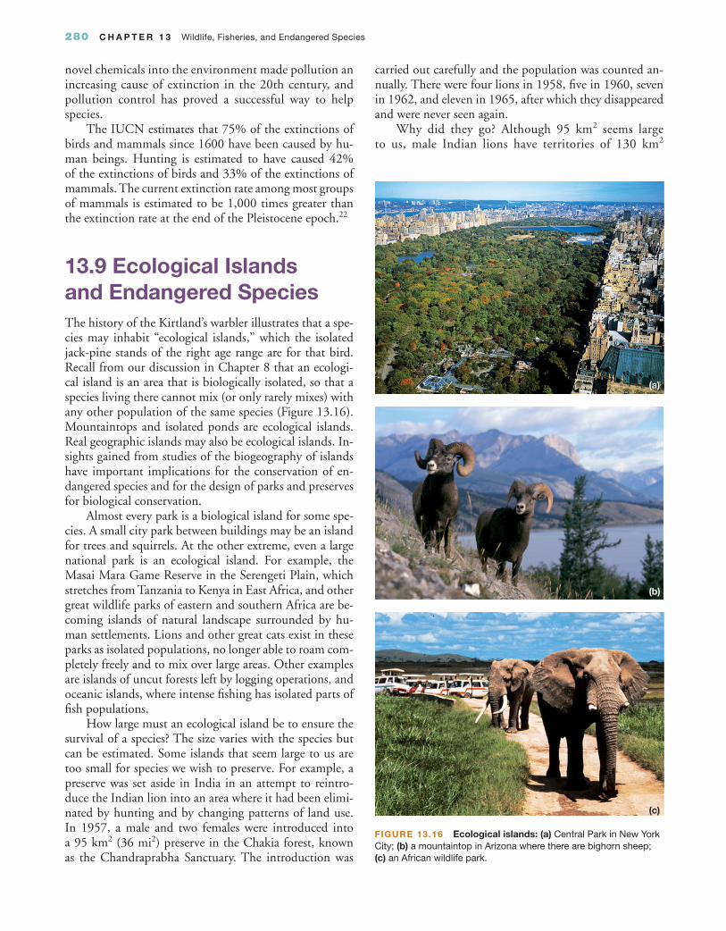
280 C H A P T E R 1 3 Wildlife, Fisheries, and Endangered Species

FIGURE 13.16 Ecological islands: (a) Central Park in New York City; (b) a mountaintop in Arizona where there are bighorn sheep; (c) an African wildlife park.

(a)

(c)

(b)

novel chemicals into the environment made pollution an increasing cause of extinction in the 20th century, and pollution control has proved a successful way to help species.

The IUCN estimates that 75% of the extinctions of birds and mammals since 1600 have been caused by hu-man beings. Hunting is estimated to have caused 42% of the extinctions of birds and 33% of the extinctions of mammals. The current extinction rate among most groups of mammals is estimated to be 1,000 times greater than the extinction rate at the end of the Pleistocene epoch.22

13.9 Ecological Islands and Endangered Species The history of the Kirtland’s warbler illustrates that a spe-cies may inhabit “ecological islands,” which the isolated jack-pine stands of the right age range are for that bird. Recall from our discussion in Chapter 8 that an ecologi-cal island is an area that is biologically isolated, so that a species living there cannot mix (or only rarely mixes) with any other population of the same species (Figure 13.16). Mountaintops and isolated ponds are ecological islands. Real geographic islands may also be ecological islands. In-sights gained from studies of the biogeography of islands have important implications for the conservation of en-dangered species and for the design of parks and preserves for biological conservation.

Almost every park is a biological island for some spe-cies. A small city park between buildings may be an island for trees and squirrels. At the other extreme, even a large national park is an ecological island. For example, the Masai Mara Game Reserve in the Serengeti Plain, which stretches from Tanzania to Kenya in East Africa, and other great wildlife parks of eastern and southern Africa are be-coming islands of natural landscape surrounded by hu-man settlements. Lions and other great cats exist in these parks as isolated populations, no longer able to roam com-pletely freely and to mix over large areas. Other examples are islands of uncut forests left by logging operations, and oceanic islands, where intense fishing has isolated parts of fish populations.

How large must an ecological island be to ensure the survival of a species? The size varies with the species but can be estimated. Some islands that seem large to us are too small for species we wish to preserve. For example, a preserve was set aside in India in an attempt to reintro-duce the Indian lion into an area where it had been elimi-nated by hunting and by changing patterns of land use. In 1957, a male and two females were introduced into a 95 km2 (36 mi2) preserve in the Chakia forest, known as the Chandraprabha Sanctuary. The introduction was

carried out carefully and the population was counted an-nually. There were four lions in 1958, five in 1960, seven in 1962, and eleven in 1965, after which they disappeared and were never seen again.

Why did they go? Although 95 km2 seems large to us, male Indian lions have territories of 130 km2

Critical Thinking Issue 281

(50 mi2), within which females and young also live. A population that could persist for a long time would need a number of such territories, so an adequate pre-serve would require 640–1,300 km2 (247–500 mi2). Various other reasons were also suggested for the disap-pearance of the lions, including poisoning and shooting by villagers. But regardless of the immediate cause, a much larger area was required for long-term persistence of the lions.

13.10 Using Spatial Relationships to Conserve Endangered Species The red-cockaded woodpecker (Figure 13.17a) is an en-dangered species of the American Southeast, numbering approximately 15,000.38 The woodpecker makes its nests in old dead or dying pines, and one of its foods is the pine bark beetle (Figure 13.17b). To conserve this species of woodpecker, these pines must be preserved. But the old pines are home to the beetles, which are pests to the trees and damage them for commercial logging. This presents an intriguing problem: How can we maintain the wood-pecker and its food (which includes the pine bark beetle) and also maintain productive forests?

The classic 20th-century way to view the relationship among the pines, the bark beetle, and the woodpecker would be to show a food chain (see Chapter 6). But this alone does not solve the problem for us. A newer approach is to consider the habitat requirements of the pine bark beetle and the woodpecker. Their requirements are some-what different, but if we overlay a map of one’s habitat

FIGURE 13.17 (a) Endangered red-cockaded woodpecker, and (b) the pine bark beetle, food for the woodpecker.

(a)

(b)

C R I T I C A L T H I N K I N G I S S U EShould Wolves Be Reestablished in the Adirondack Park?

With an area slightly over 24,000 km2, the Adirondack Park in northern New York is the largest park in the lower 48 states. Unlike most parks, however, it is a mixture of private (60%) and public (40%) land and is home to 130,000 people. When European colonists first came to the area, it was, like much of the rest of North America, inhabited by gray wolves. By 1960, wolves had been exterminated in all of the lower 48 states except for northern Minnesota. The last official sighting of a wolf in the Adirondacks was in the 1890s.

Although the gray wolf was not endangered globally—there were more than 60,000 in Canada and Alaska—it was one of the first animals listed as endangered under the 1973 Endangered Species Act. As required, the U.S. Fish and Wildlife Service developed a plan for recovery that included protection of the existing population and reintroduction of wolves to wilderness areas. The recovery plan would be consid-ered a success if survival of the Minnesota wolf population was assured and at least one other population of more than 200

requirements over a map of the other’s, we can compare the co-occurrence of habitats. Beginning with such maps, it becomes possible to design a landscape that would allow the maintenance of all three—pines, beetles, and birds.

282 C H A P T E R 1 3 Wildlife, Fisheries, and Endangered Species

wolves had been established at least 320 km from the Min-nesota population.

Under the plan, Minnesota’s wolf population increased, and some wolves from that population, as well as others from southern Canada, dispersed into northern Michigan and Wis-consin, each of which had populations of approximately 100 wolves in 1998. Also, 31 wolves from Canada were introduced into Yellowstone National Park in 1995, and that population grew to over 100. By the end of 1998, it seemed fairly certain that the criteria for removing the wolf from the Endangered Species list would soon be met.

In 1992, when the results of the recovery plan were still uncertain, the Fish and Wildlife Service proposed to investigate the possibility of reintroducing wolves to northern Maine and the Adirondack Park. A survey of New York State residents in 1996 funded by Defenders of Wildlife found that 76% of peo-ple living in the park supported reintroduction. However, many residents and organizations within the park vigorously opposed reintroduction and questioned the validity of the survey. Con-cerns focused primarily on the potential dangers to people, live-stock, and pets and the possible impact on the deer population. In response to the public outcry, Defenders of Wildlife estab-lished a citizens’ advisory committee that initiated two studies by outside experts, one on the social and economic aspects of reintroduction and another on whether there were sufficient prey and suitable habitat for wolves.

Wolves prey primarily on moose, deer, and beaver. Moose have been returning to the Adirondacks in recent years and now number about 40, but this is far less than the moose population in areas where wolves are successfully reestablishing. Beaver are abundant in the Adirondacks, with an estimated population of over 50,000. Because wolves feed on beaver primarily in the spring and the moose population is small, the main food source for Adirondack wolves would be deer.

Deer thrive in areas of early-successional forest and edge habitats, both of which have declined in the Adirondacks as log-ging has decreased on private forestland and has been eliminated altogether on public lands. Furthermore, the Adirondacks are at the northern limit of the range for white-tailed deer, where harsh winters can result in significant mortality. Deer density in the Adirondacks is estimated at 3.25 per square kilometer, fewer than in the wolf habitat in Minnesota, which also has 8,500 moose. If deer were the only prey available, wolves would kill between

2.5% and 6.5% of the deer population, while hunters take ap-proximately 13% each year. Determining whether there is a suf-ficient prey base to support a population of wolves is complicated by the fact that coyotes have moved into the Adirondacks and occupy the niche once filled by wolves. Whether wolves would add to the deer kill or replace coyotes, with no net impact on the deer population, is difficult to predict.

An area of 14,000 km2 in various parts of the Adiron-dack Park meets criteria established for suitable wolf habitat, but this is about half of the area required to maintain a wolf population for the long term. Based on the average deer den-sity and weight, as well as the food requirements of wolves, biologists estimate that this habitat could support about 155 wolves. However, human communities are scattered through-out much of the park, and many residents are concerned that wolves would not remain on public land and would threaten local residents as well as back-country hikers and hunters. Also, private lands around the edges of the park, with their greater density of deer, dairy cows, and people, could attract wolves.

Critical Thinking Questions

1. Who should make decisions about wildlife management, such as returning wolves to the Adirondacks—scientists, government officials, or the public?

2. Some people advocate leaving the decision to the wolves—that is, waiting for them to disperse from southern Canada and Maine into the Adirondacks. Study a map of the north-eastern United States and southeastern Canada. What do you think is the likelihood of natural recolonization of the Adirondacks by wolves?

3. Do you think wolves should be reintroduced to the Adiron-dack Park? If you lived in the park, would that affect your opinion? How would removal of the wolf from the Endan-gered Species list affect your opinion?

4. Some biologists recently concluded that wolves in Yellow-stone and the Great Lakes region belong to a different sub-species, the Rocky Mountain timber wolf, from those that formerly lived in the northeastern United States, the eastern timber wolf. This means that the eastern timber wolf is still extinct in the lower 48 states. Would this affect your opinion about reintroducing wolves into the Adirondacks?

S U M M A R Y

Modern approaches to management and conservation of wildlife use a broad perspective that considers inter-actions among species as well as the ecosystem and land-scape contexts. To successfully manage wildlife for harvest, conserva-tion, and protection from extinction, we need certain

quantitative information about the wildlife population, including measures of total abundance and of births and deaths, preferably recorded over a long period. The age structure of a population can also help. In addition, we have to characterize the habitat in quantitative terms. However, it is often difficult to obtain these data.

Reexamining Themes and Issues 283

R E E X A M I N I N G T H E M E S A N D I S S U E S

Global Perspective

Human Population

Sustainability

Urban World

Human beings are a primary cause of species extinctions today and also contributed to extinctions in the past. Nonindustrial societies have caused extinction by such activities as hunting and the introduction of exotic spe-cies into new habitats. With the age of exploration in the Renaissance and with the Industrial Revolution, the rate of extinctions accelerated. People altered habitats more rapidly and over greater areas. Hunting efficiency increased, as did the introduction of exotic species into new habitats. As the human population grows, conflicts over habitat between people and wildlife increase. Once again, we find that the human population prob-lem underlies this environmental issue.

At the heart of issues concerning wild living resources is the question of sustainability of species and their ecosystems. One of the key questions is whether we can sustain these resources at a constant abundance. In general, it has been assumed that fish and other wildlife that are hunted for recreation, such as deer, could be maintained at some constant, highly productive level. Constant production is desirable economically because it would provide a reliable, easily forecast income each year. But despite attempts at direct management, few wild living resources have remained at constant levels. New ideas about the intrinsic variability of ecosystems and populations lead us to question the assumption that such resources can or should be maintained at constant levels.

Although the final extinction of a species takes place in one locale, the prob-lem of biological diversity and the extinction of species is global because of the worldwide increase in the rate of extinction and because of the growth of the human population and its effects on wild living resources.

We have tended to think of wild living resources as existing outside of cities, but there is a growing recognition that urban environments will be more and more important in conserving biological diversity. This is partly because cities now occupy many sensitive habitats around the world, such as coastal and inland wetlands. It is also because appropriately designed parks and backyard plantings can provide habitats for some endangered species. As the world becomes increasingly urbanized, this function of cities will become more important.

A common goal of wildlife conservation today is to “re-store” the abundance of a species to some previous number, usually a number thought to have existed prior to the in-fluence of modern technological civilization. Information about long-ago abundances is rarely available, but some-times we can estimate numbers indirectly—for example, by using the Lewis and Clark journals to reconstruct the 1805 population of grizzly bears, or using logbooks from whaling ships. Adding to the complexity, wildlife abun-dances vary over time even in natural systems uninflu-enced by modern civilization. Also, historical information often cannot be subjected to formal tests of disproof and therefore does not by itself qualify as scientific. Adequate information exists for relatively few species.

Another approach is to seek a minimum viable popula-tion, a carrying capacity, or an optimal sustainable pop-ulation or harvest based on data that can be obtained and tested today. This approach abandons the goal of restoring a species to some hypothetical past abundance.

The good news is that many formerly endangered spe-cies have been restored to an abundance that suggests they are unlikely to become extinct. Success is achieved when the habitat is restored to conditions required by a species. The conservation and management of wildlife present great challenges but also offer great rewards of long-standing and deep meaning to people.

284 C H A P T E R 1 3 Wildlife, Fisheries, and Endangered Species

(e) wild strains of potatoes in Peru

(f ) the North American bald eagle

5. Locate an ecological island close to where you live and visit it. Which species are most vulnerable to local extinction?

6. Oysters were once plentiful in the waters around New York City. Create a plan to restore them to numbers that could be the basis for commercial harvest.

7. Using information available in libraries, determine the minimum area required for a minimum viable popula-tion of the following:

(a) domestic cats

(b) cheetahs

(c) the American alligator

(d) swallowtail butterflies

8. Both a ranch and a preserve will be established for the North American bison. The goal of the ranch owner is to show that bison can be a better source of meat than introduced cattle and at the same time have a less det-rimental effect on the land. The goal of the preserve is to maximize the abundance of the bison. How will the plans for the ranch and preserve differ, and how will they be similar?

Science and Values

People and Nature

Wildlife, fish, and endangered species are popular issues. We seem to have a deep feeling of connectedness to many wild animals—we like to watch them, and we like to know that they still exist even when we cannot see them. Wild animals have always been important symbols to people, sometimes sacred ones. The conservation of wildlife of all kinds is there-fore valuable to our sense of ourselves, both as individuals and as mem-bers of a civilization.

The reasons that people want to save endangered species begin with human values, including values placed on the continuation of life and on the public-service functions of ecosystems. Among the most con-troversial environmental issues in terms of values are the conservation of biological diversity and the protection of endangered species. Science tells us what is possible with respect to conserving species, which species are likely to persist, and which are not. Ultimately, therefore, our deci-sions about where to focus our efforts in sustaining wild living resources depend on our values.

K E Y T E R M S

carrying capacity 261catch per unit effort 265global extinction 274historical range of variation 263local extinction 274

logistic carrying capacity 261maximum sustainable yield 261maximum-sustainable-yield

population 261minimum viable population 261

optimum sustainable population 261

time series 263

S T U D Y Q U E S T I O N S

1. Why are we so unsuccessful in making rats an endangered species?

2. What have been the major causes of extinction (a) in recent times and (b) before people existed on Earth?

3. Refer back to the introductory case study about the American buffalo and grizzly bear. The U.S. Fish and Wildlife Service suggested three key indicators of the status of the grizzly bear: (1) sufficient reproduction to offset the existing levels of human-caused mor-tality, (2) adequate distribution of breeding animals throughout the area, and (3) a limit on total human-caused mortality. Are these indicators sufficient to assure the recovery of this species? What would you suggest instead?

4. This chapter discussed eight justifications for preserv-ing endangered species. Which of them apply to the following? (You can decide that none apply.)

(a) the black rhinoceros of Africa

(b) the Furbish lousewort, a rare small flowering plant of New England, seen by few people

(c) an unnamed and newly discovered beetle from the Amazon rain forest

(d) smallpox

Further Reading 285

Botkin, D.B., No Man’s Garden: Thoreau and a New Vision for Civilization and Nature (Washington, DC: Island Press, 2001). A work that discusses deep ecology and its implications for biological conservation, as well as reasons for the conserva-tion of nature, both scientific and beyond science.

Caughley, G., and A.R.E. Sinclair, Wildlife Ecology and Man-agement (London: Blackwell Scientific, 1994). A valuable text-book based on new ideas of wildlife management.

“Estimating the Abundance of Sacramento River Juvenile Win-ter Chinook Salmon with Comparisons to Adult Escape-ment,” Final Report Red Bluff Research Pumping Plant Report Series: Volume 5. Prepared by: U.S. Fish and Wildlife Service, Red Bluff Fish and Wildlife Office, 10950 Tyler Road, Red Bluff, CA 96080. Prepared for: U.S. Bureau of Reclamation,

Red Bluff Fish Passage Program, P.O. Box 159, Red Bluff, CA 96080, July.

MacKay, R., The Penguin Atlas of Endangered Species: A World-wide Guide to Plants and Animals (New York: Penguin, 2002). A geographic guide to endangered species.

Pauly, D., J. Maclean, and J.L. Maclean, The State of Fisheries and Ecosystems in the North Atlantic Ocean (Washington, DC: Island Press, 2002).

Schaller, George B., and Lu Zhi (photographers), Pandas in the Wild: Saving an Endangered Species (New York: Aperture, 2002). A photographic essay about scientists attempting to save an endangered species.

F U R T H E R R E A D I N G