Chapter 9

Tables and Information Retrieval

Tables Introduction

• In chapter 7 we showed that– By use of key comparisons alone, it is impossible

to complete a search of n items in fewer than lg n comparisons.

• Faster methods for searching ?– With an index n to locate the record of item n by

ordinary table lookup.– The time required for retrieving an entry from tab

les is O(1).

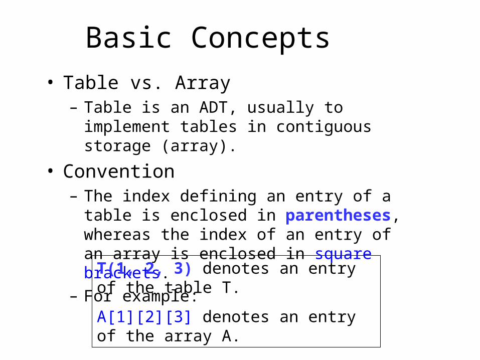
Basic Concepts• Table vs. Array

– Table is an ADT, usually to implement tables in contiguous storage (array).

• Convention– The index defining an entry of a table is enclosed

in parentheses, whereas the index of an entry of an array is enclosed in square brackets.

– For example:

T(1, 2, 3) denotes an entry of the table T.

A[1][2][3] denotes an entry of the array A.

Rectangular Tables• Rectangular Tables are so important that almost all high-

level languages provide 2-dimensional array to store and access them.

• While, computer memory space is a contiguous sequence. The machine must do some work to convert the location with in a rectangle to a position along a line.

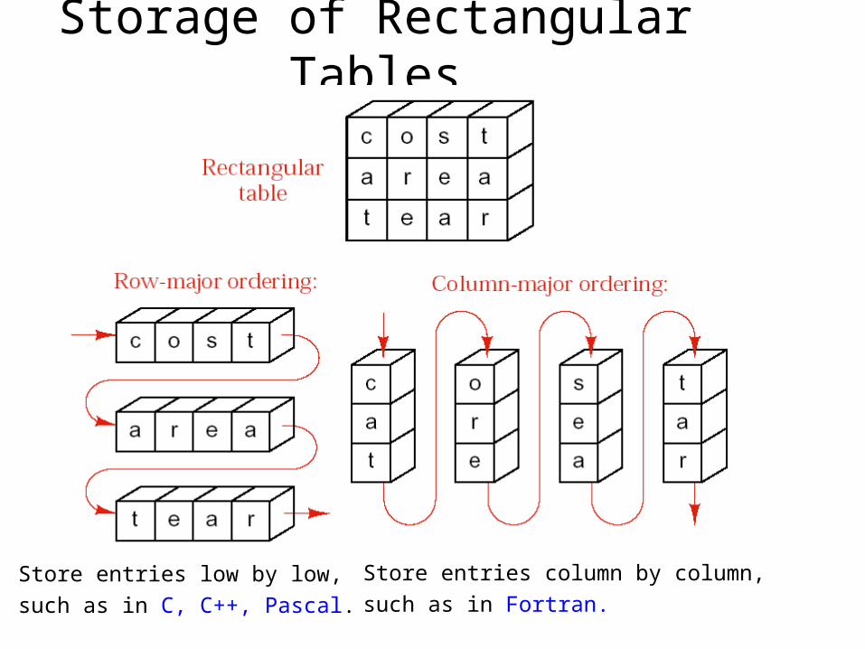
Storage of Rectangular Tables

Store entries low by low,

such as in C, C++, Pascal.

Store entries column by column,

such as in Fortran.

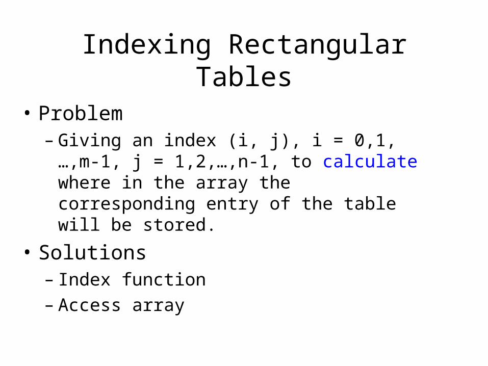
Indexing Rectangular Tables

• Problem – Giving an index (i, j), i = 0,1,…,m-1, j = 1,2,

…,n-1, to calculate where in the array the corresponding entry of the table will be stored.

• Solutions– Index function– Access array

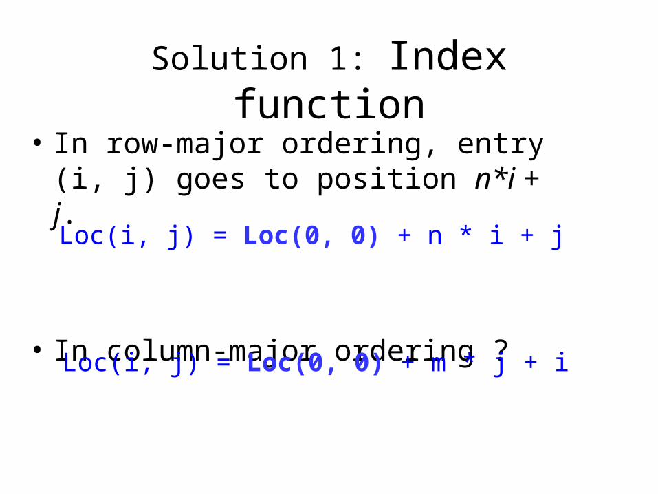
Solution 1: Index function

• In row-major ordering, entry (i, j) goes to position n*i + j.

• In column-major ordering ?

Loc(i, j) = Loc(0, 0) + n * i + j

Loc(i, j) = Loc(0, 0) + m * j + i

Solution 2: Access Array

• Access array is an auxiliary array to store some references and used to find data stored elsewhere.

Index function: Loc(i, j) = Loc(0, 0) + Accessarray[i] + j

n * i

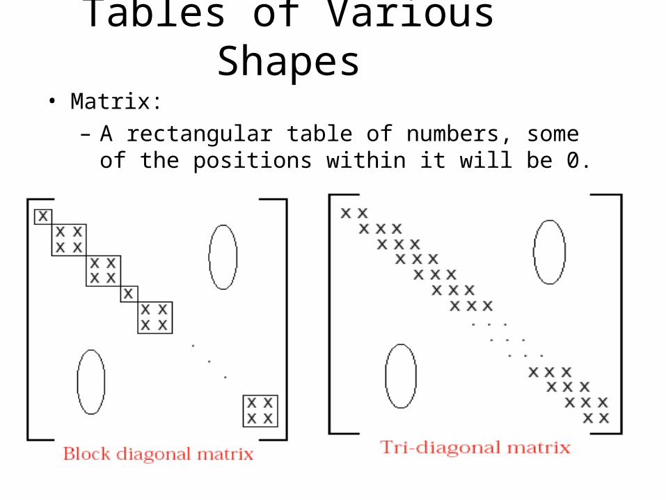
Tables of Various Shapes

• Matrix:

– A rectangular table of numbers, some of the positions within it will be 0.

Tables of Various Shapes (cont.)

• Key point– We do not need to store all entries of the

matrices in the rectangular array and leaving some position vacant. (for 0 entries)

Implementation of Matrices with Various Shapes

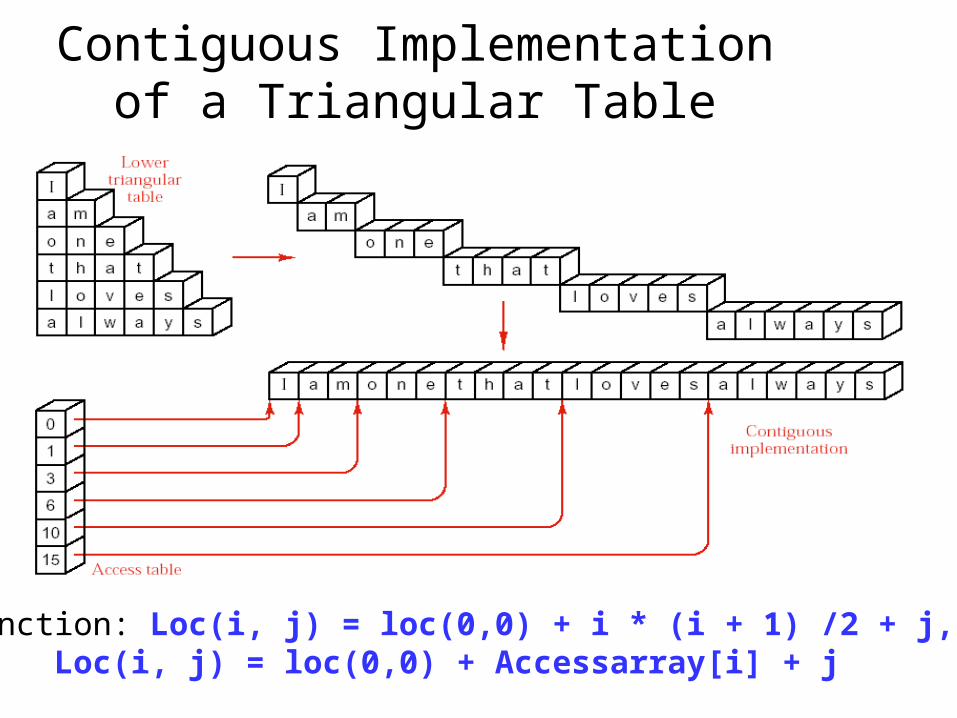
Contiguous Implementation of a Triangular Table

Index function: Loc(i, j) = loc(0,0) + i * (i + 1) /2 + j, or Loc(i, j) = loc(0,0) + Accessarray[i] + j

How about …

• ? the way to store the matrix and give the corresponding index function– Diagonal Matrix– Tri-diagonal Matrix– Upper Triangular Matrix– Symmetrically Matrix– Symmetrically Triangular Table

Exercises 9.3

Jagged Tables

• Jagged Tables– A rectangular array in which each row might have

different length.

• Jagged Table with Access Array

To set up the access array, we must construct the jagged table in its nature order, beginning with its first row.

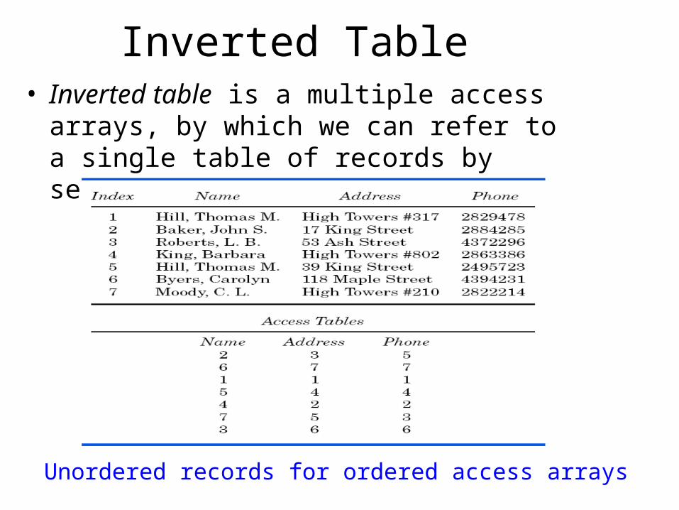
Inverted Table• Inverted table is a multiple access arrays, by

which we can refer to a single table of records by several different keys at once.

Unordered records for ordered access arrays

Formal Definition of Table

Function

Function

• In mathematics a function (函数 )is defined in terms of two sets and a correspondence from elements of the first set to elements of the second. If f is a function from a set A to a set B, then f assigns to each element of A a unique element of B.

• The set A is called the domain (定义域 ) of f , and the set B is called the codomain (值域 ) of f .

• The subset of B containing just those elements that occur as values of f is called the range (取值范围 ) of f .

ADT of Tables

Hashing

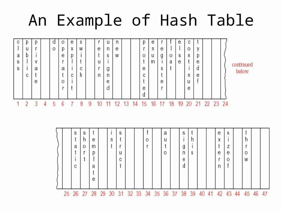
An Example of Hash Table

Hash Table• Start with an array that holds the hash table.• Use a hash function to take a key and map it to

some index in the array. – Loc = h(key), that is, loc can be seen as an index.– Since the function might map several different keys to

the same index. If the desired record is in the location given by the index, then we are finished; otherwise we must use some method to resolve the collision that may have occurred between two records wanting to go to the same location.

• To use hashing we must– (a) Find good hash functions.– (b) Determine how to resolve collisions.

Choosing a Hash Function

• A hash function should be easy and quick to compute.

• A hash function should achieve an even distribution of the keys that actually occur across the range of indices.

• A better spread of keys is often obtained by taking the size of the table (the index range) to be a prime number.

• If the hash function is poor, the performance of hashing can degenerate to that of sequential search.

Ways of Building Hash Function (1)

• Truncation– Ignore part of the key, and use the remaining

part as the index.• For example, keys are 8-digital integers, the hash

table has 1000 locations

21296876 976

– Fast, but often fail to distribute the keys evenly through the table

• Folding– Partition the key into several parts and combine

the parts in a convenient way (+ or *).• For example, keys are 8-digital integers, the hash

table has 1000 locations,

21296876 212 + 968 +76 = 1256 256

– Achieves a better spread of indices than does truncation by itself.

Ways of Building Hash Function (2)

• Modular arithmetic– Convert the key to an integer, divide by the size of the

index range, and take the remainder as the result.

– The best choice for modulus is a prime number.• For example, the hash table has 11 locations,

Loc = Key % 11

• For example, the hash table has 1000 locations,

Loc = Key % 1009

– The best way, it can achieve a good spread of indices and it ensures that the results is in the proper range.

Ways of Building Hash Function (3)

Hash function is H(key) = key mod 10, The record set is:

No. Name Class …5 Zhang c112 Liu c213 Wang c110 Li c3…

Then the hash table will be:

10 Li c3

12 Liu c2

4 Wang c15 Zhang c3

0

1

2

3

4

5

6

7

loc

key

Student No. example：

Hash function is :

C++ Example

Collision Resolutions

1) with Open Addressing (开地址法 )

2) with Chaining (链接法 )3) with Overflow Table (溢出表 )

Collision Resolution with Open Addressing (1)

• Linear Probing (线性探测法 )– Linear probing starts with the hash address and searches s

equentially for the target key or an empty position. The array should be considered circular, so that when the last location is reached, the search proceeds to the first location of the array.

– Clustering Problem• Records start to appear in long strings of adjacent positions with g

aps between the strings.

• This leads to lower hash performance and the distribution of keys become progressively more unbalanced.

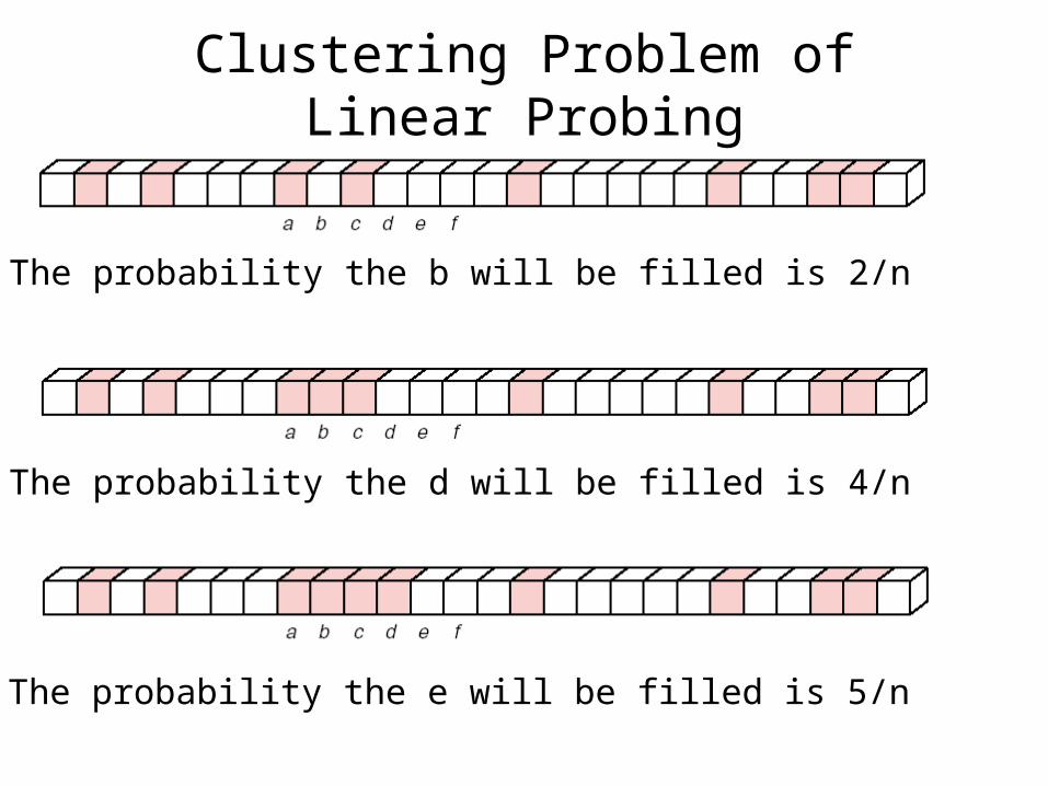
The probability the b will be filled is 2/n

The probability the d will be filled is 4/n

The probability the e will be filled is 5/n

Clustering Problem of Linear Probing

Collision Resolution with Open Addressing (2)

• Increment Functions (Rehashing)– Use a new hash function to obtain the next position to consi

der if the position is filled.– Quadratic Probing (二次探测法 )

h = h + i2, i = 1, 2, …• Quadratic probing can reduce clustering, but usually it d

oes not probe all locations in the table.• The maximum number of probes is: (hash_size+1)/2

– Random Probing (随机探测法 )

h = h + Random_number• Random probing is excellent, but slow

– Key-Dependent Increments

h = h + one character in the key

For example， h(key) = key mod 11, the size of hash table is 11. 3 records {17, 60, 29} have already put into the hash table like this:

If the fourth record with key 38 will insert, The location should be 38 mod 11=5. Now collision occurs. Where to insert it ?

60 17 290 1 2 3 4 5 6 7 8 9 10

60 17 29 380 1 2 3 4 5 6 7 8 9 10

For collision resolution with linear probing.

38 60 17 290 1 2 3 4 5 6 7 8 9 10

For collision resolution with random probing. Suppose the random number is 9.

3860 17 290 1 2 3 4 5 6 7 8 9 10

For collision resolution with quadratic probing.

Collision Resolution by Chaining

• Take the hash table itself as an array of linked list.• The linked lists from the hash table are called chains.

A chained hash table

Giving a list {19,14,23,01,68,20,84,27,55,11,10,79}.The hash function is H(key) = key mod 13. Using chaining for collision resolution. Then the corresponding hash table will be:

0123456789

101112

01 14 27 79

55 68

19 84

10 23

20

11

Count totally how many times of collision happened?

Exercise:

Characteristics of Chained Hash Table

• Advantages– If the records are large, a chained hash table can

save space.– Collision resolution with chaining is simple,

clustering is no problem.– The hash table itself can be smaller than the number

of records; overflow is no problem.– Deletion is quick and easy in a chained hash table.

• Disadvantages– If the records are very small and the table nearly

full, chaining may take more space.

• Idea– Simply put all entries that collide with occupied

location into a overflow table.– Special search method (sequence search, binary

search, etc.) could be used for overflow table.

Collision Resolution with Overflow Table

ADT of Hash Table

const int hash_size = 997; // a prime number of appropriate sizeclass Hash_table {public: Hash_table( ); void clear( ); Error_code insert(const Record &new entry); Error_code retrieve(const Key &target, Record &found) const;private: Record table[hash_size];};

• Page 409. E6.

Exercise

Analysis of Hashing

• A probe(探测 ) is one comparison of a key with the target.

• The load factor (装填因子 ) of the table isλ= n / t , where n positions are occupied out of a total of t positions in the table.

Analysis of Hashing

Analysis of Hashing

Conclusions: Comparison of Methods

• We have studied four principal methods of information retrieval– Sequential search

– Binary search

– Table lookup

– Hash-table retrieval

• The first two for lists and the second two for tables. Often we can choose either lists or tables for our data structures.

Conclusions: Comparison of Methods

• Sequential search is O(n)– Sequential search is the most flexible method. The data may be stored in

any order, with either contiguous or linked representation.

• Binary search is O(log n)– Binary search demands more, but is faster: The keys must be in order, and

the data must be in contiguous storage.

• Table lookup is O(1)– Ordinary lookup in contiguous tables is best, both in speed and

convenience, unless a list is preferred, or the set of keys is sparse, or insertions or deletions are frequent.

• Hash-table retrieval is O(1)– Hashing requires a peculiar ordering of the keys to retrieval from the hash

table, but generally useless for any other purpose.