Chapter 9 Simple Linear Regression - CMU Statisticshseltman/309/Book/chapter9.pdf · Chapter 9 Simple Linear Regression An analysis appropriate for a quantitative outcome and a single

Chapter 9

Simple Linear RegressionAn analysis appropriate for a quantitative outcome and a single quantitative ex-planatory variable.

9.1 The model behind linear regression

When we are examining the relationship between a quantitative outcome and asingle quantitative explanatory variable, simple linear regression is the most com-monly considered analysis method. (The “simple” part tells us we are only con-sidering a single explanatory variable.) In linear regression we usually have manydifferent values of the explanatory variable, and we usually assume that valuesbetween the observed values of the explanatory variables are also possible valuesof the explanatory variables. We postulate a linear relationship between the pop-ulation mean of the outcome and the value of the explanatory variable. If we letY be some outcome, and x be some explanatory variable, then we can express thestructural model using the equation

E(Y |x) = β0 + β1x

where E(), which is read “expected value of”, indicates a population mean; Y |x,which is read “Y given x”, indicates that we are looking at the possible values ofY when x is restricted to some single value; β0, read “beta zero”, is the interceptparameter; and β1, read “beta one”. is the slope parameter. A common term forany parameter or parameter estimate used in an equation for predicting Y from

213

214 CHAPTER 9. SIMPLE LINEAR REGRESSION

x is coefficient. Often the “1” subscript in β1 is replaced by the name of theexplanatory variable or some abbreviation of it.

So the structural model says that for each value of x the population mean of Y(over all of the subjects who have that particular value “x” for their explanatoryvariable) can be calculated using the simple linear expression β0 + β1x. Of coursewe cannot make the calculation exactly, in practice, because the two parametersare unknown “secrets of nature”. In practice, we make estimates of the parametersand substitute the estimates into the equation.

In real life we know that although the equation makes a prediction of the truemean of the outcome for any fixed value of the explanatory variable, it would beunwise to use extrapolation to make predictions outside of the range of x valuesthat we have available for study. On the other hand it is reasonable to interpolate,i.e., to make predictions for unobserved x values in between the observed x values.The structural model is essentially the assumption of “linearity”, at least withinthe range of the observed explanatory data.

It is important to realize that the “linear” in “linear regression” does not implythat only linear relationships can be studied. Technically it only says that thebeta’s must not be in a transformed form. It is OK to transform x or Y , and thatallows many non-linear relationships to be represented on a new scale that makesthe relationship linear.

The structural model underlying a linear regression analysis is thatthe explanatory and outcome variables are linearly related such thatthe population mean of the outcome for any x value is β0 + β1x.

The error model that we use is that for each particular x, if we have or couldcollect many subjects with that x value, their distribution around the populationmean is Gaussian with a spread, say σ2, that is the same value for each valueof x (and corresponding population mean of y). Of course, the value of σ2 isan unknown parameter, and we can make an estimate of it from the data. Theerror model described so far includes not only the assumptions of “Normality” and“equal variance”, but also the assumption of “fixed-x”. The “fixed-x” assumptionis that the explanatory variable is measured without error. Sometimes this ispossible, e.g., if it is a count, such as the number of legs on an insect, but usuallythere is some error in the measurement of the explanatory variable. In practice,

9.1. THE MODEL BEHIND LINEAR REGRESSION 215

we need to be sure that the size of the error in measuring x is small compared tothe variability of Y at any given x value. For more on this topic, see the sectionon robustness, below.

The error model underlying a linear regression analysis includes theassumptions of fixed-x, Normality, equal spread, and independent er-rors.

In addition to the three error model assumptions just discussed, we also assume“independent errors”. This assumption comes down to the idea that the error(deviation of the true outcome value from the population mean of the outcome for agiven x value) for one observational unit (usually a subject) is not predictable fromknowledge of the error for another observational unit. For example, in predictingtime to complete a task from the dose of a drug suspected to affect that time,knowing that the first subject took 3 seconds longer than the mean of all possiblesubjects with the same dose should not tell us anything about how far the nextsubject’s time should be above or below the mean for their dose. This assumptioncan be trivially violated if we happen to have a set of identical twins in the study,in which case it seems likely that if one twin has an outcome that is below the meanfor their assigned dose, then the other twin will also have an outcome that is belowthe mean for their assigned dose (whether the doses are the same or different).

A more interesting cause of correlated errors is when subjects are trained ingroups, and the different trainers have important individual differences that affectthe trainees performance. Then knowing that a particular subject does better thanaverage gives us reason to believe that most of the other subjects in the same groupwill probably perform better than average because the trainer was probably betterthan average.

Another important example of non-independent errors is serial correlationin which the errors of adjacent observations are similar. This includes adjacencyin both time and space. For example, if we are studying the effects of fertilizer onplant growth, then similar soil, water, and lighting conditions would tend to makethe errors of adjacent plants more similar. In many task-oriented experiments, ifwe allow each subject to observe the previous subject perform the task which ismeasured as the outcome, this is likely to induce serial correlation. And worst ofall, if you use the same subject for every observation, just changing the explanatory


variable each time, serial correlation is extremely likely. Breaking the assumptionof independent errors does not indicate that no analysis is possible, only that linearregression is an inappropriate analysis. Other methods such as time series methodsor mixed models are appropriate when errors are correlated.

The worst case of breaking the independent errors assumption in re-gression is when the observations are repeated measurement on thesame experimental unit (subject).

Before going into the details of linear regression, it is worth thinking about thevariable types for the explanatory and outcome variables and the relationship ofANOVA to linear regression. For both ANOVA and linear regression we assumea Normal distribution of the outcome for each value of the explanatory variable.(It is equivalent to say that all of the errors are Normally distributed.) Implic-itly this indicates that the outcome should be a continuous quantitative variable.Practically speaking, real measurements are rounded and therefore some of theircontinuous nature is not available to us. If we round too much, the variable isessentially discrete and, with too much rounding, can no longer be approximatedby the smooth Gaussian curve. Fortunately regression and ANOVA are both quiterobust to deviations from the Normality assumption, and it is OK to use discreteor continuous outcomes that have at least a moderate number of different values,e.g., 10 or more. It can even be reasonable in some circumstances to use regressionor ANOVA when the outcome is ordinal with a fairly small number of levels.

The explanatory variable in ANOVA is categorical and nominal. Imagine weare studying the effects of a drug on some outcome and we first do an experimentcomparing control (no drug) vs. drug (at a particular concentration). Regressionand ANOVA would give equivalent conclusions about the effect of drug on theoutcome, but regression seems inappropriate. Two related reasons are that thereis no way to check the appropriateness of the linearity assumption, and that aftera regression analysis it is appropriate to interpolate between the x (dose) values,and that is inappropriate here.

Now consider another experiment with 0, 50 and 100 mg of drug. Now ANOVAand regression give different answers because ANOVA makes no assumptions aboutthe relationships of the three population means, but regression assumes a linearrelationship. If the truth is linearity, the regression will have a bit more power

9.1. THE MODEL BEHIND LINEAR REGRESSION 217

0 2 4 6 8 10

05

1015

x

Y

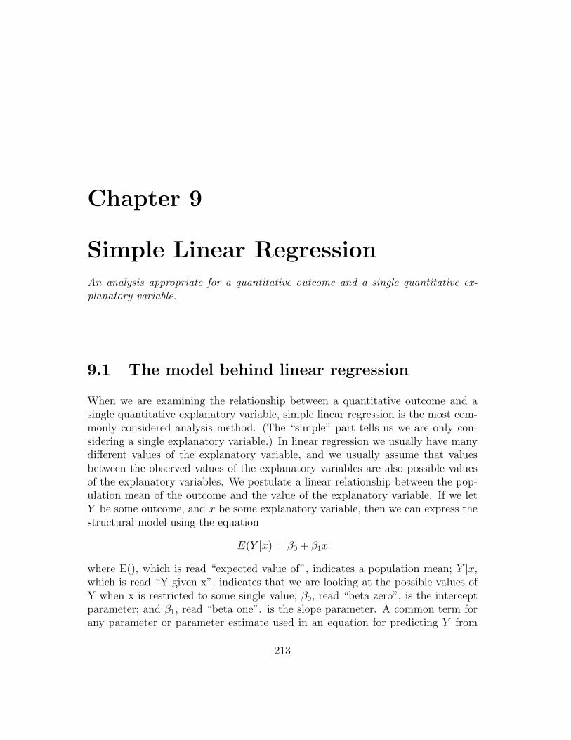
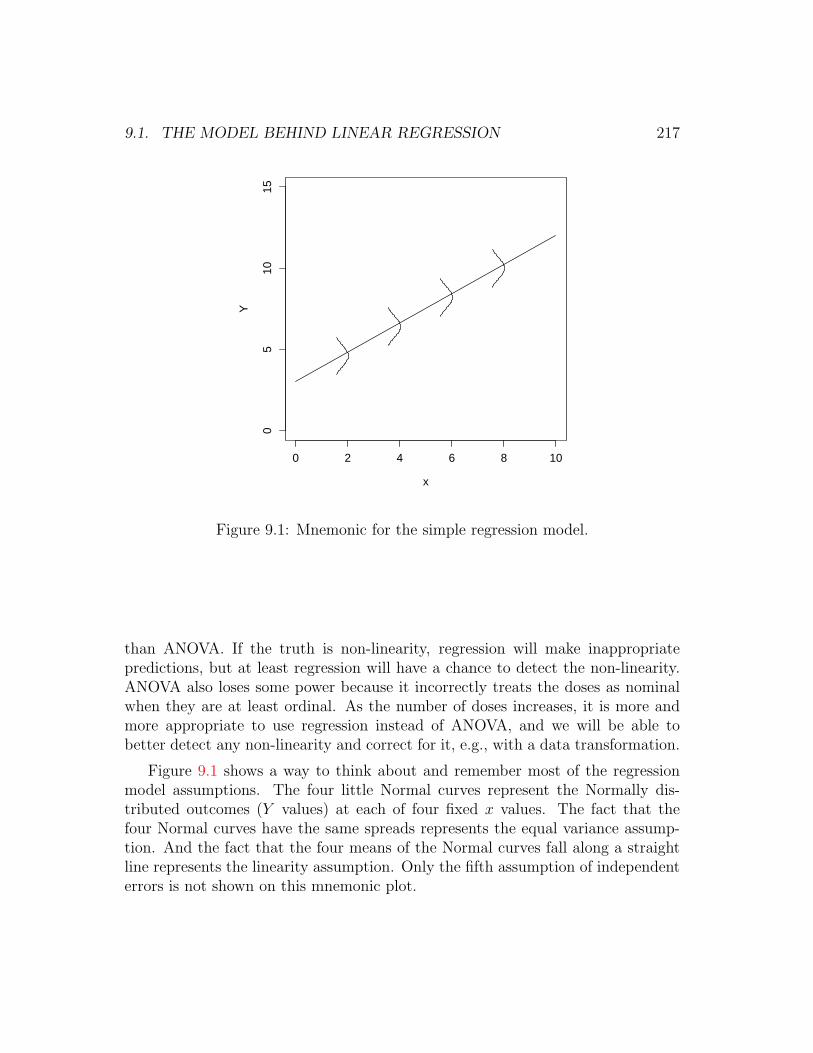
Figure 9.1: Mnemonic for the simple regression model.

than ANOVA. If the truth is non-linearity, regression will make inappropriatepredictions, but at least regression will have a chance to detect the non-linearity.ANOVA also loses some power because it incorrectly treats the doses as nominalwhen they are at least ordinal. As the number of doses increases, it is more andmore appropriate to use regression instead of ANOVA, and we will be able tobetter detect any non-linearity and correct for it, e.g., with a data transformation.

Figure 9.1 shows a way to think about and remember most of the regressionmodel assumptions. The four little Normal curves represent the Normally dis-tributed outcomes (Y values) at each of four fixed x values. The fact that thefour Normal curves have the same spreads represents the equal variance assump-tion. And the fact that the four means of the Normal curves fall along a straightline represents the linearity assumption. Only the fifth assumption of independenterrors is not shown on this mnemonic plot.


9.2 Statistical hypotheses

For simple linear regression, the chief null hypothesis is H0 : β1 = 0, and thecorresponding alternative hypothesis is H1 : β1 6= 0. If this null hypothesis is true,then, from E(Y ) = β0 + β1x we can see that the population mean of Y is β0 forevery x value, which tells us that x has no effect on Y . The alternative is thatchanges in x are associated with changes in Y (or changes in x cause changes inY in a randomized experiment).

Sometimes it is reasonable to choose a different null hypothesis for β1. For ex-ample, if x is some gold standard for a particular measurement, i.e., a best-qualitymeasurement often involving great expense, and y is some cheaper substitute, thenthe obvious null hypothesis is β1 = 1 with alternative β1 6= 1. For example, if x ispercent body fat measured using the cumbersome whole body immersion method,and Y is percent body fat measured using a formula based on a couple of skin foldthickness measurements, then we expect either a slope of 1, indicating equivalenceof measurements (on average) or we expect a different slope indicating that theskin fold method proportionally over- or under-estimates body fat.

Sometimes it also makes sense to construct a null hypothesis for β0, usuallyH0 : β0 = 0. This should only be done if each of the following is true. There aredata that span x = 0, or at least there are data points near x = 0. The statement“the population mean of Y equals zero when x = 0” both makes scientific senseand the difference between equaling zero and not equaling zero is scientificallyinteresting. See the section on interpretation below for more information.

The usual regression null hypothesis is H0 : β1 = 0. Sometimes it isalso meaningful to test H0 : β0 = 0 or H0 : β1 = 1.

9.3 Simple linear regression example

As a (simulated) example, consider an experiment in which corn plants are grown inpots of soil for 30 days after the addition of different amounts of nitrogen fertilizer.The data are in corn.dat, which is a space delimited text file with column headers.Corn plant final weight is in grams, and amount of nitrogen added per pot is in

http://www.stat.cmu.edu/~hseltman/309/Book/data/corn.dat

9.3. SIMPLE LINEAR REGRESSION EXAMPLE 219

●●

●

●

●

●

●

●

●

●

●

●

●

●

●

●

●●

●

●

●

●●

●

0 20 40 60 80 100

100

200

300

400

500

600

Soil Nitrogen (mg/pot)

Fin

al W

eigh

t (gm

)

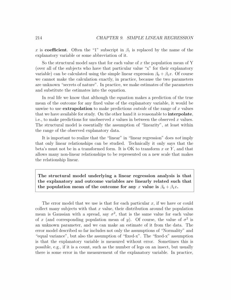
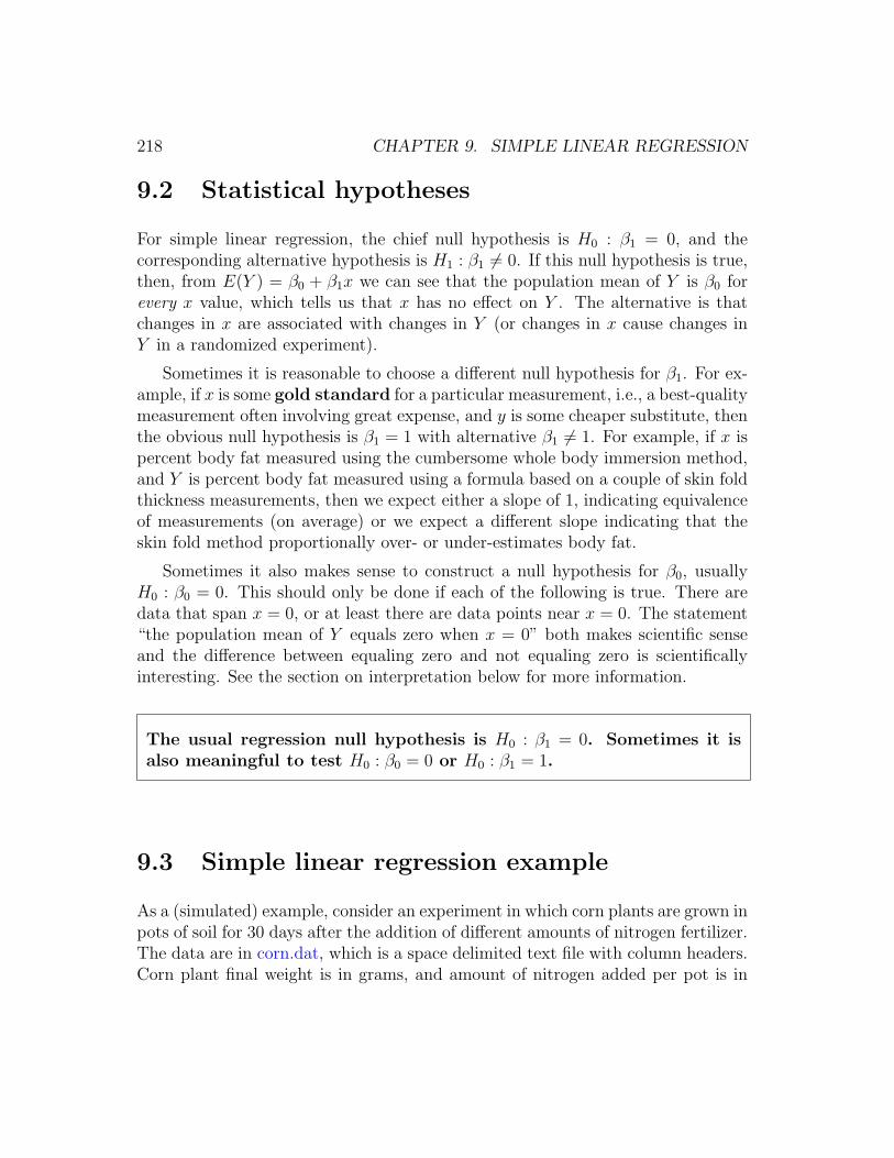
Figure 9.2: Scatterplot of corn data.

mg.

EDA, in the form of a scatterplot is shown in figure 9.2.

We want to use EDA to check that the assumptions are reasonable beforetrying a regression analysis. We can see that the assumptions of linearity seemsplausible because we can imagine a straight line from bottom left to top rightgoing through the center of the points. Also the assumption of equal spread isplausible because for any narrow range of nitrogen values (horizontally), the spreadof weight values (vertically) is fairly similar. These assumptions should only bedoubted at this stage if they are drastically broken. The assumption of Normalityis not something that human beings can test by looking at a scatterplot. But ifwe noticed, for instance, that there were only two possible outcomes in the wholeexperiment, we could reject the idea that the distribution of weights is Normal ateach nitrogen level.

The assumption of fixed-x cannot be seen in the data. Usually we just thinkabout the way the explanatory variable is measured and judge whether or not itis measured precisely (with small spread). Here, it is not too hard to measure theamount of nitrogen fertilizer added to each pot, so we accept the assumption of


fixed-x. In some cases, we can actually perform repeated measurements of x onthe same case to see the spread of x and then do the same thing for y at each ofa few values, then reject the fixed-x assumption if the ratio of x to y variance islarger than, e.g., around 0.1.

The assumption of independent error is usually not visible in the data andmust be judged by the way the experiment was run. But if serial correlation issuspected, there are tests such as the Durbin-Watson test that can be used todetect such correlation.

Once we make an initial judgement that linear regression is not a stupid thingto do for our data, based on plausibility of the model after examining our EDA, weperform the linear regression analysis, then further verify the model assumptionswith residual checking.

9.4 Regression calculations

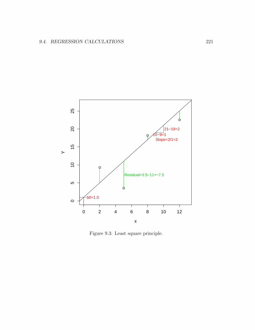
The basic regression analysis uses fairly simple formulas to get estimates of theparameters β0, β1, and σ2. These estimates can be derived from either of twobasic approaches which lead to identical results. We will not discuss the morecomplicated maximum likelihood approach here. The least squares approach isfairly straightforward. It says that we should choose as the best-fit line, that linewhich minimizes the sum of the squared residuals, where the residuals are thevertical distances from individual points to the best-fit “regression” line.

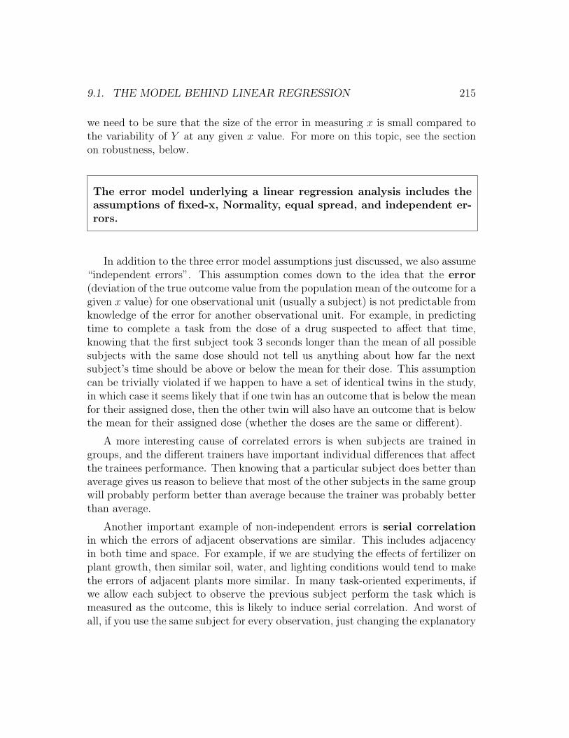
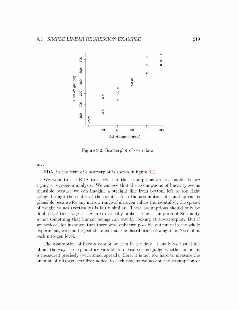
The principle is shown in figure 9.3. The plot shows a simple example withfour data points. The diagonal line shown in black is close to, but not equal to the“best-fit” line.

Any line can be characterized by its intercept and slope. The intercept is they value when x equals zero, which is 1.0 in the example. Be sure to look carefullyat the x-axis scale; if it does not start at zero, you might read off the interceptincorrectly. The slope is the change in y for a one-unit change in x. Because theline is straight, you can read this off anywhere. Also, an equivalent definition is thechange in y divided by the change in x for any segment of the line. In the figure,a segment of the line is marked with a small right triangle. The vertical change is2 units and the horizontal change is 1 unit, therefore the slope is 2/1=2. Using b0

for the intercept and b1 for the slope, the equation of the line is y = b0 + b1x.

9.4. REGRESSION CALCULATIONS 221

●

●

●

●

0 2 4 6 8 10 12

05

1015

2025

x

Y

Residual=3.5−11=−7.5

b0=1.0

10−9=121−19=2

Slope=2/1=2

Figure 9.3: Least square principle.


By plugging different values for x into this equation we can find the corre-sponding y values that are on the line drawn. For any given b0 and b1 we get apotential best-fit line, and the vertical distances of the points from the line arecalled the residuals. We can use the symbol yi, pronounced “y hat sub i”, where“sub” means subscript, to indicate the fitted or predicted value of outcome y forsubject i. (Some people also use the y′i “y-prime sub i”.) For subject i, who hasexplanatory variable xi, the prediction is yi = b0 + b1xi and the residual is yi − yi.The least square principle says that the best-fit line is the one with the smallestsum of squared residuals. It is interesting to note that the sum of the residuals(not squared) is zero for the least-squares best-fit line.

In practice, we don’t really try every possible line. Instead we use calculus tofind the values of b0 and b1 that give the minimum sum of squared residuals. Youdon’t need to memorize or use these equations, but here they are in case you areinterested.

b1 =

∑ni=1(xi − x)(yi − y)

(xi − x)2

b0 = y − b1x

Also, the best estimate of σ2 is

s2 =

∑ni=1(yi − yi)2

n− 2.

Whenever we ask a computer to perform simple linear regression, it uses theseequations to find the best fit line, then shows us the parameter estimates. Some-times the symbols β0 and β1 are used instead of b0 and b1. Even though thesesymbols have Greek letters in them, the “hat” over the beta tells us that we aredealing with statistics, not parameters.

Here are the derivations of the coefficient estimates. SSR indicates sumof squared residuals, the quantity to minimize.

SSR =n∑i=1

(yi − (β0 + β1xi))2 (9.1)

=n∑i=1

(y2i − 2yi(β0 + β1xi) + β2

0 + 2β0β1xi + β21x

2i

)(9.2)


∂SSR

∂β0

=n∑i=1

(−2yi + 2β0 + 2β1xi) (9.3)

0 =n∑i=1

(−yi + β0 + β1xi

)(9.4)

0 = −ny + nβ0 + β1nx (9.5)

β0 = y − β1x (9.6)

∂SSR

∂β1

=n∑i=1

(−2xiyi + 2β0xi + 2β1x

2i

)(9.7)

0 = −n∑i=1

xiyi + β0

n∑i=1

xi + β1

n∑i=1

x2i (9.8)

0 = −n∑i=1

xiyi + (y − β1x)n∑i=1

xi + β1

n∑i=1

x2i (9.9)

β1 =

∑ni=1 xi(yi − y)∑ni=1 xi(xi − x)

(9.10)

A little algebra shows that this formula for β1 is equivalent to the oneshown above because c

∑ni=1(zi − z) = c · 0 = 0 for any constant c and

variable z.

In multiple regression, the matrix formula for the coefficient estimates is(X ′X)−1X ′y, where X is the matrix with all ones in the first column (forthe intercept) and the values of the explanatory variables in subsequentcolumns.

Because the intercept and slope estimates are statistics, they have samplingdistributions, and these are determined by the true values of β0, β1, and σ2, aswell as the positions of the x values and the number of subjects at each x value.If the model assumptions are correct, the sampling distributions of the interceptand slope estimates both have means equal to the true values, β0 and β1, andare Normally distributed with variances that can be calculated according to fairlysimple formulas which involve the x values and σ2.

In practice, we have to estimate σ2 with s2. This has two consequences. Firstwe talk about the standard errors of the sampling distributions of each of the betas


instead of the standard deviations, because, by definition, SE’s are estimates ofs.d.’s of sampling distributions. Second, the sampling distribution of bj − βj (forj=0 or 1) is now the t-distribution with n − 2 df (see section 3.9.5), where n isthe total number of subjects. (Loosely we say that we lose two degrees of freedombecause they are used up in the estimation of the two beta parameters.) Using thenull hypothesis of βj = 0 this reduces to the null sampling distribution bj ∼ tn−2.

The computer will calculate the standard errors of the betas, the t-statisticvalues, and the corresponding p-values (for the usual two-sided alternative hypoth-esis). We then compare these p-values to our pre-chosen alpha (usually α = 0.05)to make the decisions whether to retain or reject the null hypotheses.

The formulas for the standard errors come from the formula for thevariance covariance matrix of the joint sampling distributions of β0 andβ1 which is σ2(X ′X)−1, where X is the matrix with all ones in the firstcolumn (for the intercept) and the values of the explanatory variable inthe second column. This formula also works in multiple regression wherethere is a column for each explanatory variable. The standard errors of thecoefficients are obtained by substituting s2 for the unknown σ2 and takingthe square roots of the diagonal elements.

For simple regression this reduces to

SE(b0) = s

√√√√ ∑x2

n∑

(x2)− (∑x)2

and

SE(b1) = s

√n

n∑

(x2)− (∑x)2

.

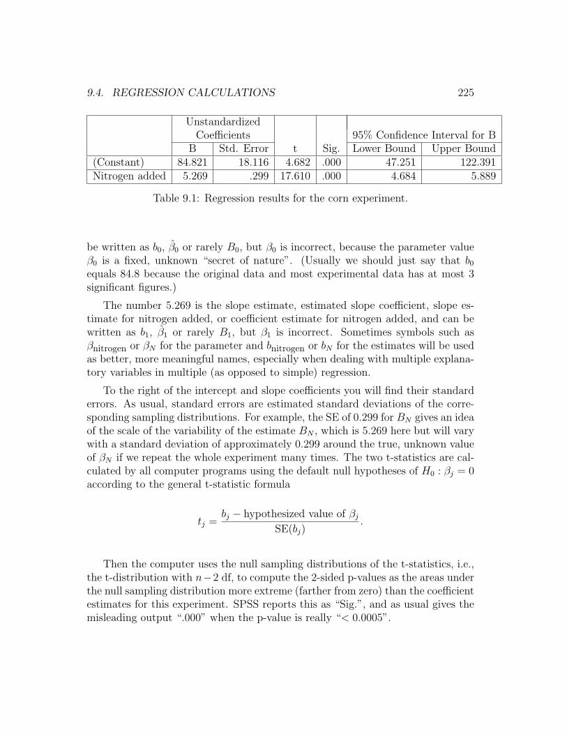
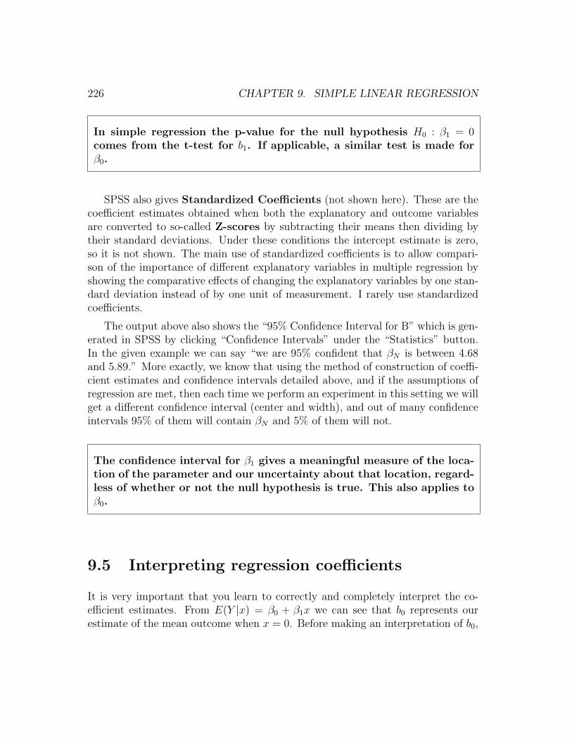
The basic regression output is shown in table 9.1 in a form similar to thatproduced by SPSS, but somewhat abbreviated. Specifically, “standardized coeffi-cients” are not included.

In this table we see the number 84.821 to the right of the “(Constant)” labeland under the labels “Unstandardized Coefficients” and “B”. This is called theintercept estimate, estimated intercept coefficient, or estimated constant, and can


UnstandardizedCoefficients 95% Confidence Interval for B

B Std. Error t Sig. Lower Bound Upper Bound(Constant) 84.821 18.116 4.682 .000 47.251 122.391Nitrogen added 5.269 .299 17.610 .000 4.684 5.889

Table 9.1: Regression results for the corn experiment.

be written as b0, β0 or rarely B0, but β0 is incorrect, because the parameter valueβ0 is a fixed, unknown “secret of nature”. (Usually we should just say that b0

equals 84.8 because the original data and most experimental data has at most 3significant figures.)

The number 5.269 is the slope estimate, estimated slope coefficient, slope es-timate for nitrogen added, or coefficient estimate for nitrogen added, and can bewritten as b1, β1 or rarely B1, but β1 is incorrect. Sometimes symbols such asβnitrogen or βN for the parameter and bnitrogen or bN for the estimates will be usedas better, more meaningful names, especially when dealing with multiple explana-tory variables in multiple (as opposed to simple) regression.

To the right of the intercept and slope coefficients you will find their standarderrors. As usual, standard errors are estimated standard deviations of the corre-sponding sampling distributions. For example, the SE of 0.299 for BN gives an ideaof the scale of the variability of the estimate BN , which is 5.269 here but will varywith a standard deviation of approximately 0.299 around the true, unknown valueof βN if we repeat the whole experiment many times. The two t-statistics are cal-culated by all computer programs using the default null hypotheses of H0 : βj = 0according to the general t-statistic formula

tj =bj − hypothesized value of βj

SE(bj).

Then the computer uses the null sampling distributions of the t-statistics, i.e.,the t-distribution with n−2 df, to compute the 2-sided p-values as the areas underthe null sampling distribution more extreme (farther from zero) than the coefficientestimates for this experiment. SPSS reports this as “Sig.”, and as usual gives themisleading output “.000” when the p-value is really “< 0.0005”.


In simple regression the p-value for the null hypothesis H0 : β1 = 0comes from the t-test for b1. If applicable, a similar test is made forβ0.

SPSS also gives Standardized Coefficients (not shown here). These are thecoefficient estimates obtained when both the explanatory and outcome variablesare converted to so-called Z-scores by subtracting their means then dividing bytheir standard deviations. Under these conditions the intercept estimate is zero,so it is not shown. The main use of standardized coefficients is to allow compari-son of the importance of different explanatory variables in multiple regression byshowing the comparative effects of changing the explanatory variables by one stan-dard deviation instead of by one unit of measurement. I rarely use standardizedcoefficients.

The output above also shows the “95% Confidence Interval for B” which is gen-erated in SPSS by clicking “Confidence Intervals” under the “Statistics” button.In the given example we can say “we are 95% confident that βN is between 4.68and 5.89.” More exactly, we know that using the method of construction of coeffi-cient estimates and confidence intervals detailed above, and if the assumptions ofregression are met, then each time we perform an experiment in this setting we willget a different confidence interval (center and width), and out of many confidenceintervals 95% of them will contain βN and 5% of them will not.

The confidence interval for β1 gives a meaningful measure of the loca-tion of the parameter and our uncertainty about that location, regard-less of whether or not the null hypothesis is true. This also applies toβ0.

9.5 Interpreting regression coefficients

It is very important that you learn to correctly and completely interpret the co-efficient estimates. From E(Y |x) = β0 + β1x we can see that b0 represents ourestimate of the mean outcome when x = 0. Before making an interpretation of b0,

9.5. INTERPRETING REGRESSION COEFFICIENTS 227

first check the range of x values covered by the experimental data. If there is nox data near zero, then the intercept is still needed for calculating y and residualvalues, but it should not be interpreted because it is an extrapolated value.

If there are x values near zero, then to interpret the intercept you must expressit in terms of the actual meanings of the outcome and explanatory variables. Forthe example of this chapter, we would say that b0 (84.8) is the estimated corn plantweight (in grams) when no nitrogen is added to the pots (which is the meaning ofx = 0). This point estimate is of limited value, because it does not express thedegree of uncertainty associated with it. So often it is better to use the CI for b0.In this case we say that we are 95% confident that the mean weight for corn plantswith no added nitrogen is between 47 and 122 gm, which is quite a wide range. (Itwould be quite misleading to report the mean no-nitrogen plant weight as 84.821gm because it gives a false impression of high precision.)

After interpreting the estimate of b0 and it’s CI, you should consider whetherthe null hypothesis, β0 = 0 makes scientific sense. For the corn example, the nullhypothesis is that the mean plant weight equals zero when no nitrogen is added.Because it is unreasonable for plants to weigh nothing, we should stop here and notinterpret the p-value for the intercept. For another example, consider a regressionof weight gain in rats over a 6 week period as it relates to dose of an anabolicsteroid. Because we might be unsure whether the rats were initially at a stableweight, it might make sense to test H0 : β0 = 0. If the null hypothesis is rejectedthen we conclude that it is not true that the weight gain is zero when the dose iszero (control group), so the initial weight was not a stable baseline weight.

Interpret the estimate, b0, only if there are data near zero and settingthe explanatory variable to zero makes scientific sense. The meaningof b0 is the estimate of the mean outcome when x = 0, and shouldalways be stated in terms of the actual variables of the study. The p-value for the intercept should be interpreted (with respect to retainingor rejecting H0 : β0 = 0) only if both the equality and the inequality ofthe mean outcome to zero when the explanatory variable is zero arescientifically plausible.

For interpretation of a slope coefficient, this section will assume that the settingis a randomized experiment, and conclusions will be expressed in terms of causa-


tion. Be sure to substitute association if you are looking at an observational study.The general meaning of a slope coefficient is the change in Y caused by a one-unitincrease in x. It is very important to know in what units x are measured, so thatthe meaning of a one-unit increase can be clearly expressed. For the corn experi-ment, the slope is the change in mean corn plant weight (in grams) caused by a onemg increase in nitrogen added per pot. If a one-unit change is not substantivelymeaningful, the effect of a larger change should be used in the interpretation. Forthe corn example we could say the a 10 mg increase in nitrogen added causes a52.7 gram increase in plant weight on average. We can also interpret the CI forβ1 in the corn experiment by saying that we are 95% confident that the change inmean plant weight caused by a 10 mg increase in nitrogen is 46.8 to 58.9 gm.

Be sure to pay attention to the sign of b1. If it is positive then b1 represents theincrease in outcome caused by each one-unit increase in the explanatory variable. Ifb1 is negative, then each one-unit increase in the explanatory variable is associatedwith a fall in outcome of magnitude equal to the absolute value of b1.

A significant p-value indicates that we should reject the null hypothesis thatβ1 = 0. We can express this as evidence that plant weight is affected by changesin nitrogen added. If the null hypothesis is retained, we should express this ashaving no good evidence that nitrogen added affects plant weight. Particularly inthe case of when we retain the null hypothesis, the interpretation of the CI for β1

is better than simply relying on the general meaning of retain.

The interpretation of b1 is the change (increase or decrease dependingon the sign) in the average outcome when the explanatory variableincreases by one unit. This should always be stated in terms of theactual variables of the study. Retention of the null hypothesis H0 : β1 =0 indicates no evidence that a change in x is associated with (or causesfor a randomized experiment) a change in y. Rejection indicates thatchanges in x cause changes in y (assuming a randomized experiment).

9.6. RESIDUAL CHECKING 229

9.6 Residual checking

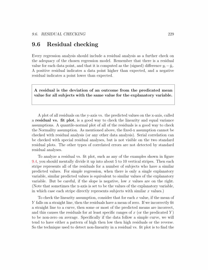
Every regression analysis should include a residual analysis as a further check onthe adequacy of the chosen regression model. Remember that there is a residualvalue for each data point, and that it is computed as the (signed) difference yi− yi.A positive residual indicates a data point higher than expected, and a negativeresidual indicates a point lower than expected.

A residual is the deviation of an outcome from the predicated meanvalue for all subjects with the same value for the explanatory variable.

A plot of all residuals on the y-axis vs. the predicted values on the x-axis, calleda residual vs. fit plot, is a good way to check the linearity and equal varianceassumptions. A quantile-normal plot of all of the residuals is a good way to checkthe Normality assumption. As mentioned above, the fixed-x assumption cannot bechecked with residual analysis (or any other data analysis). Serial correlation canbe checked with special residual analyses, but is not visible on the two standardresidual plots. The other types of correlated errors are not detected by standardresidual analyses.

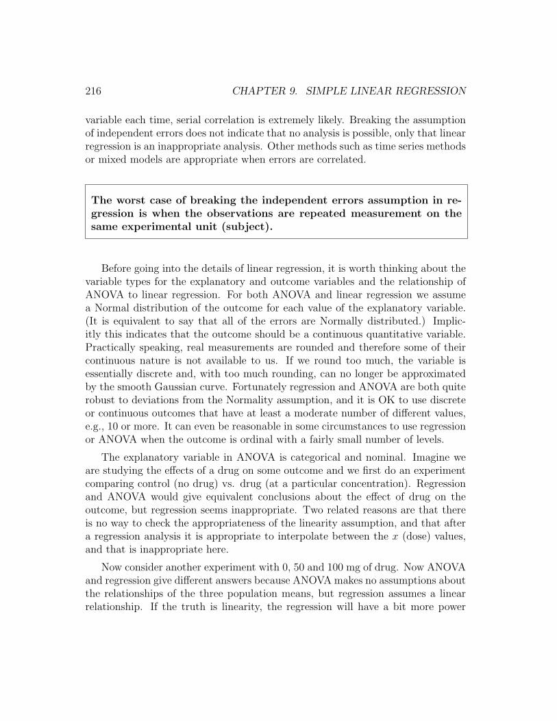
To analyze a residual vs. fit plot, such as any of the examples shown in figure9.4, you should mentally divide it up into about 5 to 10 vertical stripes. Then eachstripe represents all of the residuals for a number of subjects who have a similarpredicted values. For simple regression, when there is only a single explanatoryvariable, similar predicted values is equivalent to similar values of the explanatoryvariable. But be careful, if the slope is negative, low x values are on the right.(Note that sometimes the x-axis is set to be the values of the explanatory variable,in which case each stripe directly represents subjects with similar x values.)

To check the linearity assumption, consider that for each x value, if the mean ofY falls on a straight line, then the residuals have a mean of zero. If we incorrectly fita straight line to a curve, then some or most of the predicted means are incorrect,and this causes the residuals for at least specific ranges of x (or the predicated Y )to be non-zero on average. Specifically if the data follow a simple curve, we willtend to have either a pattern of high then low then high residuals or the reverse.So the technique used to detect non-linearity in a residual vs. fit plot is to find the


●

●

●

●

●

●

●

●

●

●

●

●

●

●

●

●

●

●●

●●

●● ●

●

●

●

●

●

●

●

●

●

●

●

●

●

●

●

●

●

●●

●

●

●●

●

●

●

20 40 60 80 100

−10

−5

05

A

Fitted value

Res

idua

l

●

●

●

●

●

●●

●

●

●● ●

●

●

●

●

●

●

●

●

●

●

●

●

● ●

●

●

●

● ●

●

●

●

●

●

●●

●

●

●●

●

●

●

●

●

●●

●

20 40 60 80 100

−10

−5

05

10

B

Fitted value

Res

idua

l●

●

●

●

●

●

●

●

●

●●

● ●

●●

●

●

●

●

●

●

●

●

●

●

●

●

●

●

●

●●

●

●

●

●

●

●

●

●●

●●●

●

●

●

●●

●

20 25 30 35

−15

−5

515

C

Fitted value

Res

idua

l

●

●

●●

●●

●

●

●

●

●

●

●

●

●

●

●

●●

●

●

●

●

●●

●

●

●

●

●

●

●

●

●

●

●

●

●

●

●

●

●

●

●

●

●

●

●

●

●

0 20 60 100

−10

010

20

D

Fitted value

Res

idua

l

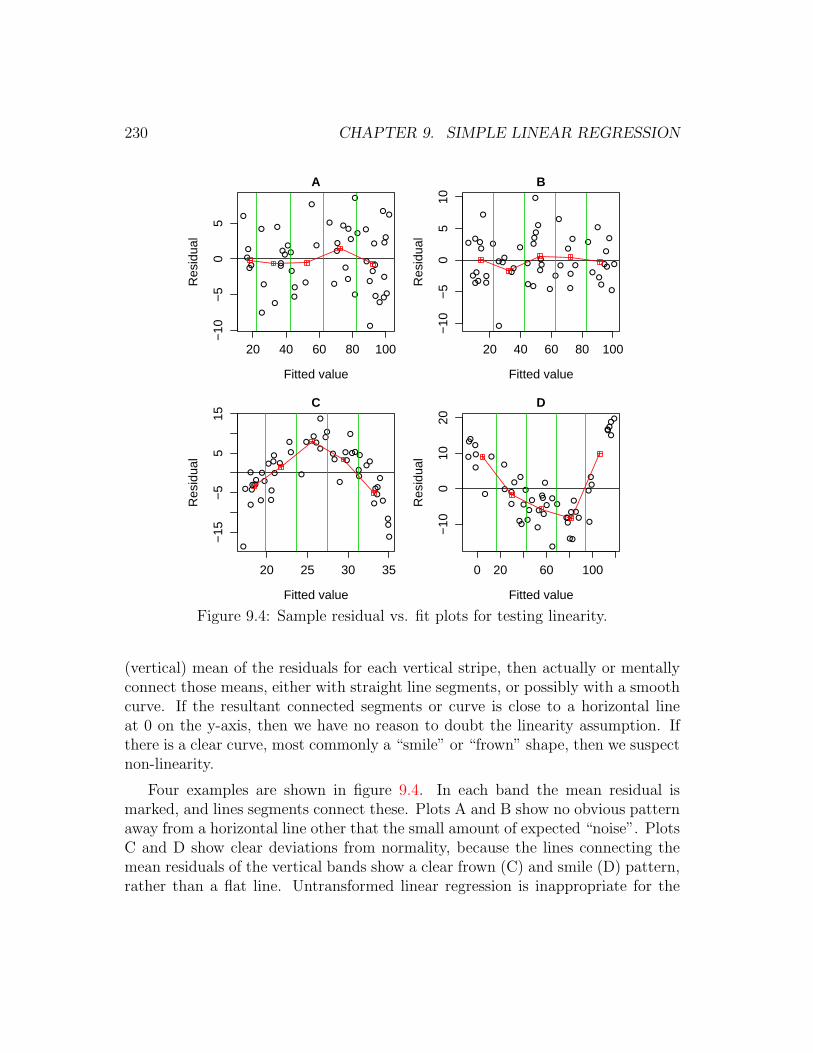
Figure 9.4: Sample residual vs. fit plots for testing linearity.

(vertical) mean of the residuals for each vertical stripe, then actually or mentallyconnect those means, either with straight line segments, or possibly with a smoothcurve. If the resultant connected segments or curve is close to a horizontal lineat 0 on the y-axis, then we have no reason to doubt the linearity assumption. Ifthere is a clear curve, most commonly a “smile” or “frown” shape, then we suspectnon-linearity.

Four examples are shown in figure 9.4. In each band the mean residual ismarked, and lines segments connect these. Plots A and B show no obvious patternaway from a horizontal line other that the small amount of expected “noise”. PlotsC and D show clear deviations from normality, because the lines connecting themean residuals of the vertical bands show a clear frown (C) and smile (D) pattern,rather than a flat line. Untransformed linear regression is inappropriate for the

9.6. RESIDUAL CHECKING 231

●

●

●

●

●

●

●●

●

●●

●

●●

●

●●●

●

●

●

●

●

●

●

●

●

●

●

●

●

●

●

●

●

●

●

●

● ●

●

●

●

●

●

●●

●

●

●●

●●

●●

●●

●

●

●

●

●●

●

●

●

●

●

●

●● ●

●

●

●

●

●●

●

●

20 40 60 80 100

−5

05

10

A

Fitted value

Res

idua

l

●●

●

●

●

●

●

●

●

●

●

●

●

●

●●

●

●

●

●

●

●

●

●

●●

●

●

●●

●

●●

●

●

●●

●

●

●

●

● ●●

●

●●●

●

●

●

●

●

●

●

●

●

●

●●

●

●

●

●

●

●

●

●

●

●

●

●

●

●

●

● ●

●

●

●

0 20 40 60 80 100

−10

−5

05

10

B

Fitted value

Res

idua

l

●

●●

●

●

●

●

●●

●

●

●●

●

●● ●

●●

●● ●

●

●● ●

●

●

●

●

●●

● ●

●

●

●●

●

●●●

●

●

●

●●

●

●●

●

●

●

●

●

●

●●

●

●

●●●

●

●

●

●

●

●

●

●

●

●

●

●

●●

●

●

●

20 40 60 80 100

−10

00

5010

0

C

Fitted value

Res

idua

l

●

●

●●

●

●

● ●●●

●

●

●

●●

●

●

●●

●

●

●

●

●

●

●

●●

●●

●●

●

●●

●

● ●

●●

●

●●

●

●●

●

●

●

●

●● ●

●●

●

●

●

●●

● ●●●

●

●

●

●

●

●

●

●

●●

●

●

●

●

●

●

0 20 40 60 80

−10

00

50

D

Fitted value

Res

idua

l

Figure 9.5: Sample residual vs. fit plots for testing equal variance.

data that produced plots C and D. With practice you will get better at readingthese plots.

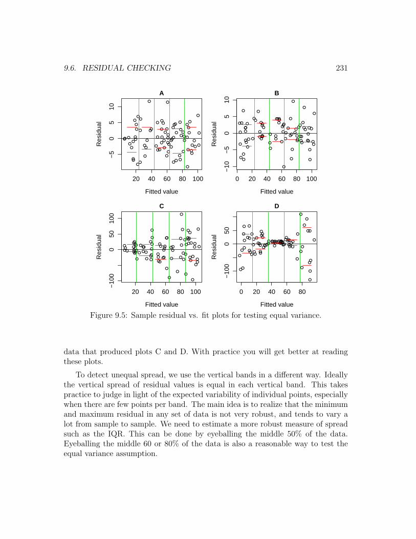
To detect unequal spread, we use the vertical bands in a different way. Ideallythe vertical spread of residual values is equal in each vertical band. This takespractice to judge in light of the expected variability of individual points, especiallywhen there are few points per band. The main idea is to realize that the minimumand maximum residual in any set of data is not very robust, and tends to vary alot from sample to sample. We need to estimate a more robust measure of spreadsuch as the IQR. This can be done by eyeballing the middle 50% of the data.Eyeballing the middle 60 or 80% of the data is also a reasonable way to test theequal variance assumption.


Figure 9.5 shows four residual vs. fit plots, each of which shows good linearity.The red horizontal lines mark the central 60% of the residuals. Plots A and B showno evidence of unequal variance; the red lines are a similar distance apart in eachband. In plot C you can see that the red lines increase in distance apart as youmove from left to right. This indicates unequal variance, with greater variance athigh predicted values (high x values if the slope is positive). Plot D show a patternwith unequal variance in which the smallest variance is in the middle of the rangeof predicted values, with larger variance at both ends. Again, this takes practice,but you should at least recognize obvious patterns like those shown in plots C andD. And you should avoid over-reading the slight variations seen in plots A and B.

The residual vs. fit plot can be used to detect non-linearity and/orunequal variance.

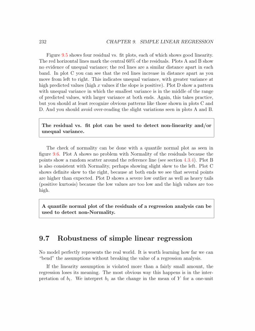
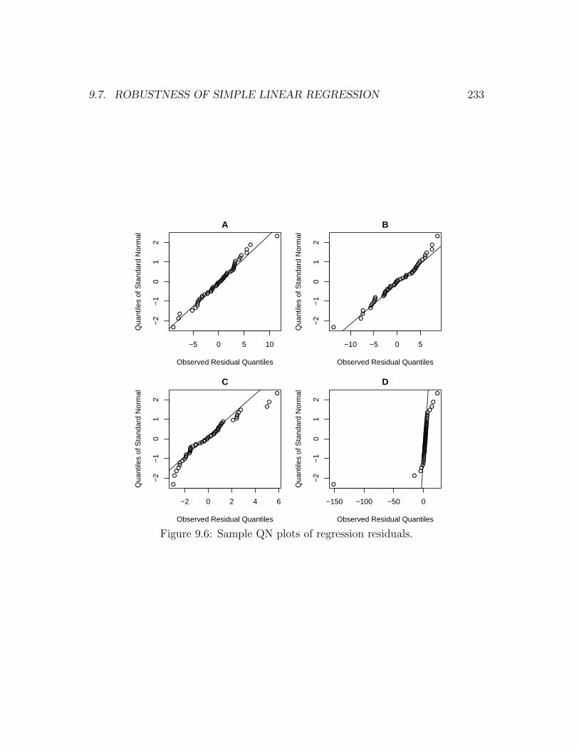
The check of normality can be done with a quantile normal plot as seen infigure 9.6. Plot A shows no problem with Normality of the residuals because thepoints show a random scatter around the reference line (see section 4.3.4). Plot Bis also consistent with Normality, perhaps showing slight skew to the left. Plot Cshows definite skew to the right, because at both ends we see that several pointsare higher than expected. Plot D shows a severe low outlier as well as heavy tails(positive kurtosis) because the low values are too low and the high values are toohigh.

A quantile normal plot of the residuals of a regression analysis can beused to detect non-Normality.

9.7 Robustness of simple linear regression

No model perfectly represents the real world. It is worth learning how far we can“bend” the assumptions without breaking the value of a regression analysis.

If the linearity assumption is violated more than a fairly small amount, theregression loses its meaning. The most obvious way this happens is in the inter-pretation of b1. We interpret b1 as the change in the mean of Y for a one-unit

9.7. ROBUSTNESS OF SIMPLE LINEAR REGRESSION 233

●

●

●

●

●

●

●

●

●

●

●●

●●●

●

●

●

●

●

●

●●

●

●

●

●

●

●

●

●

●

●

●●

●

●

●

●

●

●

●

●

●

●

●●

●

●

●

−5 0 5 10

−2

−1

01

2

A

Observed Residual Quantiles

Qua

ntile

s of

Sta

ndar

d N

orm

al

●

●

●

●

●

●

●●

●●

●●

●●

●●

●

●

●

●

●●

●●

●

●

●

●

●

●

●●

●

●

●

●

●

●

●

●

●

●

●

●

●

●

●

●

●

●

−10 −5 0 5

−2

−1

01

2

B


Qua

ntile

s of

Sta

ndar

d N

orm

al

●

●

●●

●

●

●

●

●

●

●

●

● ●

●

●

●

●

●

●

●

●

●

●

●

●

●

●

●

●●

●

●●

●

●●●

●●●

●

●

●

●●

●

●

●

●

−2 0 2 4 6

−2

−1

01

2

C


Qua

ntile

s of

Sta

ndar

d N

orm

al

●

●

●●

●●

●

●

●

●

●●

●

●

●

●

●

●

●

●

●

●

●

●

●●

●

●

●

●

●

●●

●

●

●

●●

●

●●

●

●

●

●

●

●●

●

●

−150 −100 −50 0

−2

−1

01

2

D


Qua

ntile

s of

Sta

ndar

d N

orm

al

Figure 9.6: Sample QN plots of regression residuals.


increase in x. If the relationship between x and Y is curved, then the change inY for a one-unit increase in x varies at different parts of the curve, invalidatingthe interpretation. Luckily it is fairly easy to detect non-linearity through EDA(scatterplots) and/or residual analysis. If non-linearity is detected, you should tryto fix it by transforming the x and/or y variables. Common transformations arelog and square root. Alternatively it is common to add additional new explanatoryvariables in the form of a square, cube, etc. of the original x variable one at a timeuntil the residual vs. fit plot shows linearity of the residuals. For data that canonly lie between 0 and 1, it is worth knowing (but not memorizing) that the squareroot of the arcsine of y is often a good transformation.

You should not feel that transformations are “cheating”. The original waythe data is measured usually has some degree of arbitrariness. Also, commonmeasurements like pH for acidity, decibels for sound, and the Richter earthquakescale are all log scales. Often transformed values are transformed back to theoriginal scale when results are reported (but the fact that the analysis was on atransformed scale must also be reported).

Regression is reasonably robust to the equal variance assumption. Moderatedegrees of violation, e.g., the band with the widest variation is up to twice as wideas the band with the smallest variation, tend to cause minimal problems. For moresevere violations, the p-values are incorrect in the sense that their null hypothesestend to be rejected more that 100α% of the time when the null hypothesis is true.The confidence intervals (and the SE’s they are based on) are also incorrect. Forworrisome violations of the equal variance assumption, try transformations of they variable (because the assumption applies at each x value, transformation of xwill be ineffective).

Regression is quite robust to the Normality assumption. You only need to worryabout severe violations. For markedly skewed or kurtotic residual distributions,we need to worry that the p-values and confidence intervals are incorrect. In thatcase try transforming the y variable. Also, in the case of data with less than ahandful of different y values or with severe truncation of the data (values pilingup at the ends of a limited width scale), regression may be inappropriate due tonon-Normality.

The fixed-x assumption is actually quite important for regression. If the vari-ability of the x measurement is of similar or larger magnitude to the variability ofthe y measurement, then regression is inappropriate. Regression will tend to givesmaller than correct slopes under these conditions, and the null hypothesis on the

9.8. ADDITIONAL INTERPRETATION OF REGRESSION OUTPUT 235

slope will be retained far too often. Alternate techniques are required if the fixed-xassumption is broken, including so-called Type 2 regression or “errors in variablesregression”.

The independent errors assumption is also critically important to regression.A slight violation, such as a few twins in the study doesn’t matter, but other mildto moderate violations destroy the validity of the p-value and confidence intervals.In that case, use alternate techniques such as the paired t-test, repeated measuresanalysis, mixed models, or time series analysis, all of which model correlated errorsrather than assume zero correlation.

Regression analysis is not very robust to violations of the linearity,fixed-x, and independent errors assumptions. It is somewhat robustto violation of equal variance, and moderately robust to violation ofthe Normality assumption.

9.8 Additional interpretation of regression out-

put

Regression output usually includes a few additional components beyond the slopeand intercept estimates and their t and p-values.

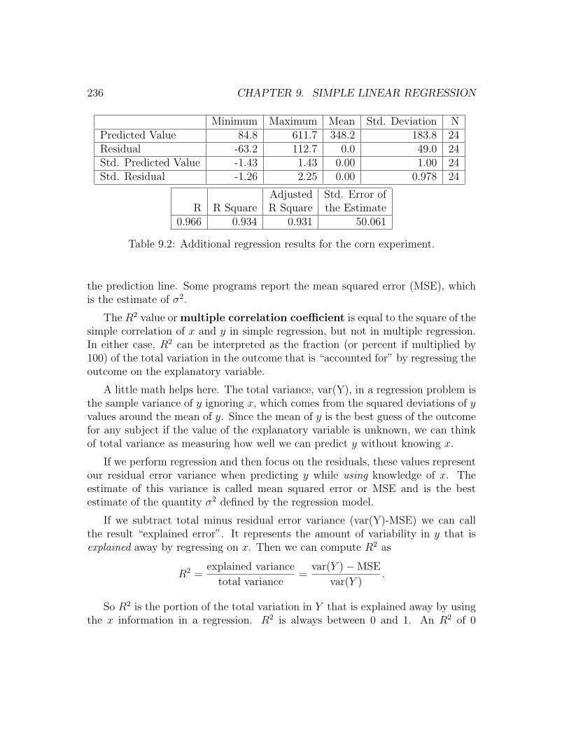
Additional regression output is shown in table 9.2 which has what SPSS labels“Residual Statistics” on top and what it labels “Model Summary” on the bottom.The Residual Statistics summarize the predicted (fit) and residual values, as wellas “standardized” values of these. The standardized values are transformed to Z-scores. You can use this table to detect possible outliers. If you know a lot aboutthe outcome variable, use the unstandardized residual information to see if theminimum, maximum or standard deviation of the residuals is more extreme thanyou expected. If you are less familiar, standardized residuals bigger than about 3in absolute value suggest that those points may be outliers.

The “Standard Error of the Estimate”, s, is the best estimate of σ from ourmodel (on the standard deviation scale). So it represents how far data will fallfrom the regression predictions on the scale of the outcome measurements. For thecorn analysis, only about 5% of the data falls more than 2(49)=98 gm away from


Minimum Maximum Mean Std. Deviation NPredicted Value 84.8 611.7 348.2 183.8 24Residual -63.2 112.7 0.0 49.0 24Std. Predicted Value -1.43 1.43 0.00 1.00 24Std. Residual -1.26 2.25 0.00 0.978 24

Adjusted Std. Error ofR R Square R Square the Estimate

0.966 0.934 0.931 50.061

Table 9.2: Additional regression results for the corn experiment.

the prediction line. Some programs report the mean squared error (MSE), whichis the estimate of σ2.

The R2 value or multiple correlation coefficient is equal to the square of thesimple correlation of x and y in simple regression, but not in multiple regression.In either case, R2 can be interpreted as the fraction (or percent if multiplied by100) of the total variation in the outcome that is “accounted for” by regressing theoutcome on the explanatory variable.

A little math helps here. The total variance, var(Y), in a regression problem isthe sample variance of y ignoring x, which comes from the squared deviations of yvalues around the mean of y. Since the mean of y is the best guess of the outcomefor any subject if the value of the explanatory variable is unknown, we can thinkof total variance as measuring how well we can predict y without knowing x.

If we perform regression and then focus on the residuals, these values representour residual error variance when predicting y while using knowledge of x. Theestimate of this variance is called mean squared error or MSE and is the bestestimate of the quantity σ2 defined by the regression model.

If we subtract total minus residual error variance (var(Y)-MSE) we can callthe result “explained error”. It represents the amount of variability in y that isexplained away by regressing on x. Then we can compute R2 as

R2 =explained variance

total variance=

var(Y )−MSE

var(Y ).

So R2 is the portion of the total variation in Y that is explained away by usingthe x information in a regression. R2 is always between 0 and 1. An R2 of 0

9.9. USING TRANSFORMATIONS 237

means that x provides no information about y. An R2 of 1 means that use ofx information allows perfect prediction of y with every point of the scatterplotexactly on the regression line. Anything in between represents different levels ofcloseness of the scattered points around the regression line.

So for the corn problem we can say the 93.4% of the total variation in plantweight can be explained by regressing on the amount of nitrogen added. Unfortu-nately, there is no clear general interpretation of the values of R2. While R2 = 0.6might indicate a great finding in social sciences, it might indicate a very poorfinding in a chemistry experiment.

R2 is a measure of the fraction of the total variation in the outcomethat can be explained by the explanatory variable. It runs from 0 to1, with 1 indicating perfect prediction of y from x.

9.9 Using transformations

If you find a problem with the equal variance or Normality assumptions, you willprobably want to see if the problem goes away if you use log(y) or y2 or

√y or 1/y

instead of y for the outcome. (It never matters whether you choose natural vs.common log.) For non-linearity problems, you can try transformation of x, y, orboth. If regression on the transformed scale appears to meet the assumptions oflinear regression, then go with the transformations. In most cases, when reportingyour results, you will want to back transform point estimates and the ends ofconfidence intervals for better interpretability. By “back transform” I mean dothe inverse of the transformation to return to the original scale. The inverse ofcommon log of y is 10y; the inverse of natural log of y is ey; the inverse of y2 is√y; the inverse of

√y is y2; and the inverse of 1/y is 1/y again. Do not transform

a p-value – the p-value remains unchanged.

Here are a couple of examples of transformation and how the interpretations ofthe coefficients are modified. If the explanatory variable is dose of a drug and theoutcome is log of time to complete a task, and b0 = 2 and b1 = 1.5, then we cansay the best estimate of the log of the task time when no drug is given is 2 or thatthe the best estimate of the time is 102 = 100 or e2 = 7.39 depending on which log


was used. We also say that for each 1 unit increase in drug, the log of task timeincreases by 1.5 (additively). On the original scale this is a multiplicative increaseof 101.5 = 31.6 or e1.5 = 4.48. Assuming natural log, this says every time the dosegoes up by another 1 unit, the mean task time get multiplied by 4.48.

If the explanatory variable is common log of dose and the outcome is bloodsugar level, and b0 = 85 and b1 = 18 then we can say that when log(dose)=0,blood sugar is 85. Using 100 = 1, this tells us that blood sugar is 85 when doseequals 1. For every 1 unit increase in log dose, the glucose goes up by 18. But aone unit increase in log dose is a ten fold increase in dose (e.g., dose from 10 to 100is log dose from 1 to 2). So we can say that every time the dose increases 10-foldthe glucose goes up by 18.

Transformations of x or y to a different scale are very useful for fixingbroken assumptions.

9.10 How to perform simple linear regression in

SPSS

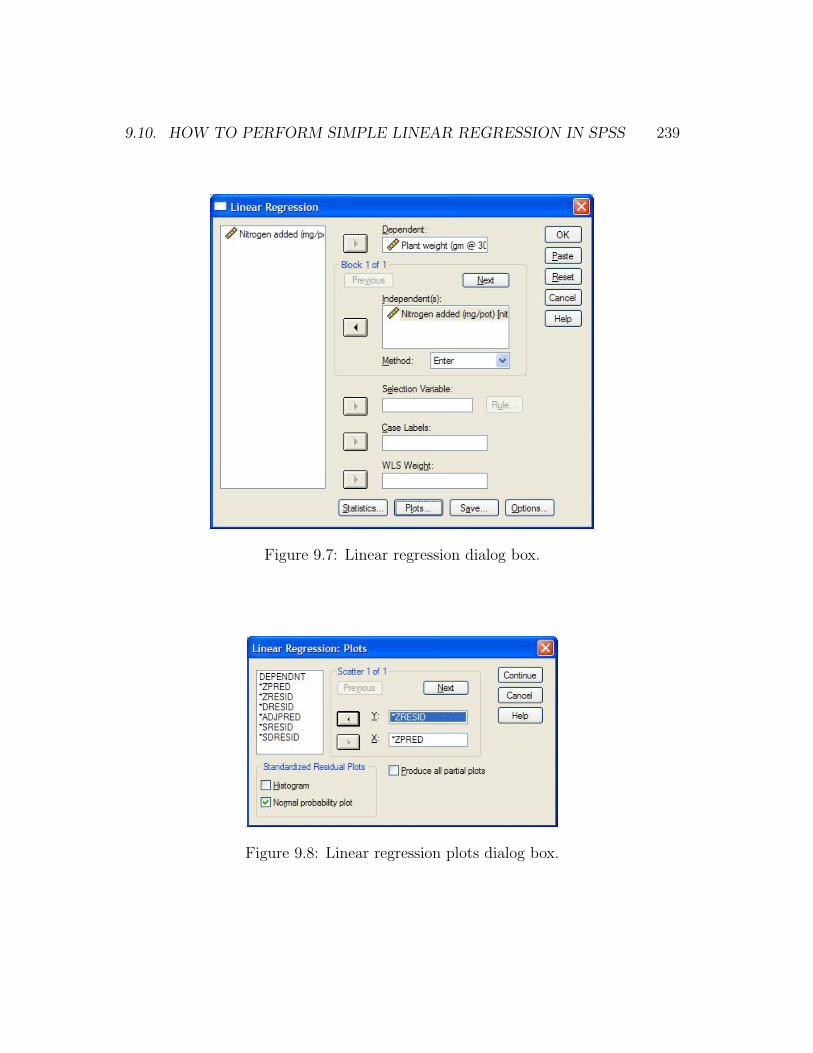
To perform simple linear regression in SPSS, select Analyze/Regression/Linear...from the menu. You will see the “Linear Regression” dialog box as shown in figure9.7. Put the outcome in the “Dependent” box and the explanatory variable in the“Independent(s)” box. I recommend checking the “Confidence intervals” box for“Regression Coefficients” under the “Statistics...” button. Also click the “Plots...”button to get the “Linear Regression: Plots” dialog box shown in figure 9.8. Fromhere under “Scatter” put “*ZRESID” into the “Y” box and “*ZPRED” into the“X” box to produce the residual vs. fit plot. Also check the “Normal probabilityplot” box.

9.10. HOW TO PERFORM SIMPLE LINEAR REGRESSION IN SPSS 239

Figure 9.7: Linear regression dialog box.

Figure 9.8: Linear regression plots dialog box.


In a nutshell: Simple linear regression is used to explore the relation-ship between a quantitative outcome and a quantitative explanatoryvariable. The p-value for the slope, b1, is a test of whether or notchanges in the explanatory variable really are associated with changesin the outcome. The interpretation of the confidence interval for β1 isusually the best way to convey what has been learned from a study.Occasionally there is also interest in the intercept. No interpretationsshould be given if the assumptions are violated, as determined bythinking about the fixed-x and independent errors assumptions, andchecking the residual vs. fit and residual QN plots for the other threeassumptions.

Documents

Chapter 9 Simple Linear Regression - CMU Statisticshseltman/309/Book/chapter9.pdf · Chapter 9 Simple Linear Regression An analysis appropriate for a quantitative outcome and a single