Chapter 9 Slidesnebula2.deanza.edu/~mo/Math10/ch09.pdf · Chapter 9 Slides Maurice Geraghty, 2018 6 Using Box Plot to find outliers The “box” is the region between the 1stand

Chapter 9 Slides

Maurice Geraghty, 2018 1

Inferential Statistics and Probabilitya Holistic Approach

1

Chapter 9One Population Hypothesis

Testing

This Course Material by Maurice Geraghty is licensed under a Creative Commons Attribution-ShareAlike 4.0 International License.

Conditions for use are shown here: https://creativecommons.org/licenses/by-sa/4.0/

Procedures of Hypotheses Testing

2

Hypotheses Testing – Procedure 1

3

General Research Question Decide on a topic or phenomena that you want to

research. Formulate general research questions based on the

topic

4

topic. Example:

Topic: Health Care Reform Some General Questions:

Would a Single Payer Plan be less expensive than Private Insurance? Do HMOs provide the same quality care as PPOs? Would the public support mandated health coverage?

EXAMPLE – General Question

A food company has a policy that the stated contents of a product match the actual results.

A General Question might be “Does the stated net

9-13

5

A General Question might be Does the stated net weight of a food product match (on average) the actual weight?”

The quality control statistician could then decide to test various food products for accuracy.


6

Chapter 9 Slides


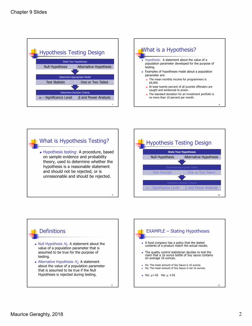
Hypothesis Testing DesignState Your Hypotheses

Null Hypothesis Alternative Hypothesis

7

Determine Decision Criteria

α – Significance Level β and Power Analysis

Determine Appropriate Model

Test Statistic One or Two Tailed

What is a Hypothesis? Hypothesis: A statement about the value of a

population parameter developed for the purpose of testing.

Examples of hypotheses made about a population

9-3

8

a p es o ypot eses ade about a popu at oparameter are: The mean monthly income for programmers is

$9,000. At least twenty percent of all juvenile offenders are

caught and sentenced to prison. The standard deviation for an investment portfolio is

no more than 10 percent per month.

What is Hypothesis Testing?

Hypothesis testing: A procedure, based on sample evidence and probability theory, used to determine whether the

9-4

9

theory, used to determine whether the hypothesis is a reasonable statement and should not be rejected, or is unreasonable and should be rejected.



10





Definitions

Null Hypothesis H0: A statement about the value of a population parameter that is assumed to be true for the purpose of

9-6

11

assumed to be true for the purpose of testing.

Alternative Hypothesis Ha: A statement about the value of a population parameter that is assumed to be true if the Null Hypothesis is rejected during testing.

EXAMPLE – Stating Hypotheses


The quality control statistician decides to test the

9-13

The quality control statistician decides to test the claim that a 16 ounce bottle of Soy sauce contains on average 16 ounces.

Ho: The mean amount of Soy Sauce is 16 ounces Ha: The mean amount of Soy Sauce is not 16 ounces.

Ho: μ=16 Ha: μ ≠16

12

Chapter 9 Slides




13





Definitions Statistical Model: A mathematical model that describes the

behavior of the data being tested. Normal Family = the Standard Normal Distribution (Z) and

functions of independent Standard Normal Distributions

9-7

14

(eg: t, χ2, F). Most Statistical Models will be from the Normal Family due

to the Central Limit Theorem. Model Assumptions: Criteria which must be satisfied to

appropriately use a chosen Statistical Model. Test statistic: A value, determined from sample information,

used to determine whether or not to reject the null hypothesis.

EXAMPLE – Choosing Model

The quality control statistician decides to test the claim that a 16 ounce bottle of Soy sauce contains on average 16 ounces. We will assume the population standard is known

Ho: μ=16 Ha: μ ≠16

9-13

Ho: μ=16 Ha: μ ≠16

Model: One sample test Z test of mean

Test Statistic:

15

0XZn

μσ

−=



16





Definitions

Level of Significance: The probability of rejecting the null hypothesis when it is actually true (signified by )

9-6

17

actually true. (signified by α) Type I Error: Rejecting the null

hypothesis when it is actually true. Type II Error: Failing to reject the null

hypothesis when it is actually false.

Outcomes of Hypothesis Testing

Fail to Reject Ho Reject Ho

18

Ho is true Correct Decision Type I error

Ho is False Type II error Correct Decision

Chapter 9 Slides


EXAMPLE – Type I and Type II Errors

Ho: The mean amount of Soy Sauce is 16 ounces Ha: The mean amount of Soy Sauce is not 16 ounces.

Type I Error: The researcher supports the claim that the t f i t 16 h th t l

9-13

mean amount of soy sauce is not 16 ounces when the actual mean is 16 ounces. The company needlessly “fixes” a machine that is operating properly.

Type II Error: The researcher fails to support the claim that the mean amount of soy sauce is not 16 ounces when the actual mean is not 16 ounces. The company fails to fix a machine that is not operating properly.

19



20





Definitions

Critical value(s): The dividing point(s) between the region where the null hypothesis is rejected and the

9-7

21

region where it is not rejected. The critical value determines the decision rule.

Rejection Region: Region(s) of the Statistical Model which contain the values of the Test Statistic where the Null Hypothesis will be rejected. The area of the Rejection Region = α

One-Tailed Tests of Significance A test is one-tailed when the alternate

hypothesis, Ha , states a direction, such as: H0 : The mean income of females is less than or equal to the

mean income of males.

9-8

22

Ha : The mean income of females is greater than males. Equality is part of H0 Ha determines which tail to test

Ha: μ>μ0 means test upper tail. Ha: μ<μ0 means test lower tail.

One-tailed test

HH

a μμμμ

0

00

::

>

≤

23

n

XZ

a

σμ

αμμ

0

0

05.−=

=

Two-Tailed Tests of Significance A test is two-tailed when no direction is

specified in the alternate hypothesis Ha , such as: H0 : The mean income of females is equal to the mean

9-10

24

H0 : The mean income of females is equal to the mean income of males.

Ha : The mean income of females is not equal to the mean income of the males.

Equality is part of H0 Ha determines which tail to test

Ha: μ≠μ0 means test both tails.

Chapter 9 Slides


Two-tailed test

HH

a μμμμ

0

00

::

≠

=

25

n

XZ

a

σμ

αα

0

0

025.205.

−=

==


26

Collect and Analyze Experimental Data

Collect and Verify Data

Conduct Experiment Check for Outliers

27

Make a Decision about Ho

Reject Ho and support Ha Fail to Reject Ho

Determine Test Statistic and/or p-value

Compare to Critical Value Compare to α




28





Outliers An outlier is data point that is far

removed from the other entries in the data set.

29

data set. Outliers could be

Mistakes made in recording data Data that don’t belong in population True rare events

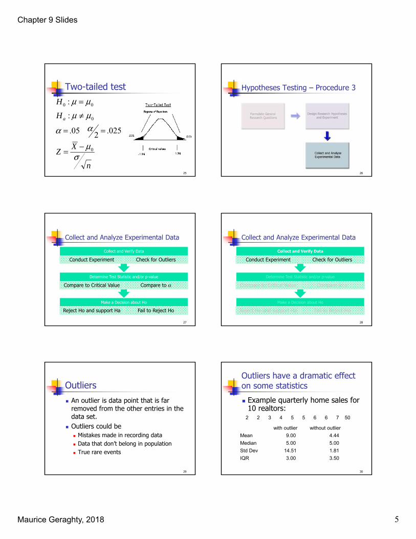
Outliers have a dramatic effect on some statistics Example quarterly home sales for

10 realtors:2 2 3 4 5 5 6 6 7 50

30

2 2 3 4 5 5 6 6 7 50

with outlier without outlierMean 9.00 4.44 Median 5.00 5.00 Std Dev 14.51 1.81 IQR 3.00 3.50

Chapter 9 Slides


Using Box Plot to find outliers The “box” is the region between the 1st and 3rd quartiles. Possible outliers are more than 1.5 IQR’s from the box (inner fence) Probable outliers are more than 3 IQR’s from the box (outer fence) In the box plot below, the dotted lines represent the “fences” that are

31

p p1.5 and 3 IQR’s from the box. See how the data point 50 is well outside the outer fence and therefore an almost certain outlier.

Using Z-score to detect outliers Calculate the mean and standard deviation

without the suspected outlier. Calculate the Z-score of the suspected

32

outlier. If the Z-score is more than 3 or less than -3,

that data point is a probable outlier.

2.2581.1

4.450 =−=Z

Outliers – what to do Remove or not remove, there is no clear answer.

For some populations, outliers don’t dramatically change the overall statistical analysis. Example: the tallest person in the

ld ill t d ti ll h th h i ht f 10000

33

world will not dramatically change the mean height of 10000 people.

However, for some populations, a single outlier will have a dramatic effect on statistical analysis (called “Black Swan” by Nicholas Taleb) and inferential statistics may be invalid in analyzing these populations. Example: the richest person in the world will dramatically change the mean wealth of 10000 people.

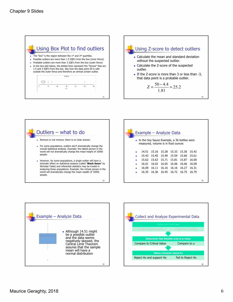
Example – Analyze Data In the Soy Sauce Example, a 36 bottles were

measured, volume is in fluid ounces

14 51 15 16 15 28 15 33 15 36 15 42 14.51 15.16 15.28 15.33 15.36 15.42 15.43 15.45 15.49 15.59 15.60 15.61 15.62 15.63 15.71 15.81 15.87 16.00 16.01 16.02 16.05 16.06 16.06 16.09 16.09 16.11 16.16 16.16 16.27 16.31 16.35 16.36 16.45 16.72 16.75 16.79

34

Example – Analyze Data

Although 14.51 might be a possible outlierbe a possible outlier and the data seems negatively skewed, the Central Limit Theorem assures that the sample mean will have a normal distribution

35




36





Chapter 9 Slides


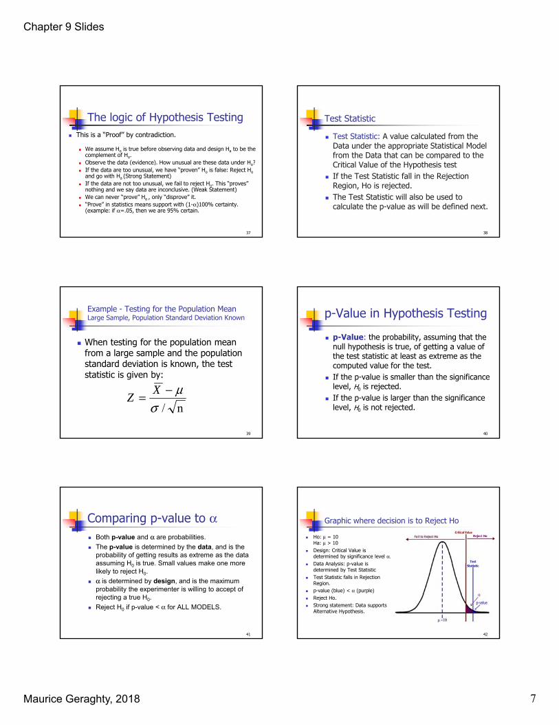
The logic of Hypothesis Testing This is a “Proof” by contradiction.

We assume Ho is true before observing data and design Ha to be the complement of Ho.Observe the data (evidence) How unusual are these data under H ?

37

Observe the data (evidence). How unusual are these data under Ho? If the data are too unusual, we have “proven” Ho is false: Reject Ho

and go with Ha (Strong Statement) If the data are not too unusual, we fail to reject Ho. This “proves”

nothing and we say data are inconclusive. (Weak Statement) We can never “prove” Ho , only “disprove” it. “Prove” in statistics means support with (1-α)100% certainty.

(example: if α=.05, then we are 95% certain.

Test Statistic

Test Statistic: A value calculated from the Data under the appropriate Statistical Model from the Data that can be compared to the

l l f h hCritical Value of the Hypothesis test If the Test Statistic fall in the Rejection

Region, Ho is rejected. The Test Statistic will also be used to

calculate the p-value as will be defined next.

38

Example - Testing for the Population MeanLarge Sample, Population Standard Deviation Known

When testing for the population mean from a large sample and the population standard deviation is known the test

9-12

39

standard deviation is known, the test statistic is given by:

n/σμ−= XZ

p-Value in Hypothesis Testing p-Value: the probability, assuming that the

null hypothesis is true, of getting a value of the test statistic at least as extreme as the

d l f h

9-15

40

computed value for the test. If the p-value is smaller than the significance

level, H0 is rejected. If the p-value is larger than the significance

level, H0 is not rejected.

Comparing p-value to α Both p-value and α are probabilities. The p-value is determined by the data, and is the

probability of getting results as extreme as the data assuming H is true Small values make one more

41

assuming H0 is true. Small values make one more likely to reject H0.

α is determined by design, and is the maximum probability the experimenter is willing to accept of rejecting a true H0.

Reject H0 if p-value < α for ALL MODELS.

Graphic where decision is to Reject Ho

Ho: μ = 10 Ha: μ > 10

Design: Critical Value is determined by significance level α.Data Analysis: p value is Data Analysis: p-value is determined by Test Statistic

Test Statistic falls in Rejection Region.

p-value (blue) < α (purple) Reject Ho. Strong statement: Data supports

Alternative Hypothesis.

42

Chapter 9 Slides


Graphic where decision is Fail to Reject Ho

Ho: μ = 10 Ha: μ > 10

Design: Critical Value is determined by significance level α.Data Analysis: p value is Data Analysis: p-value is determined by Test Statistic

Test Statistic falls in Non-rejection Region.

p-value (blue) > α (purple) Fail to Reject Ho. Weak statement: Data is

inconclusive and does not support Alternative Hypothesis.

43

EXAMPLE – General Question


A General Question might be “Does the stated net

9-13

44

A General Question might be Does the stated net weight of a food product match the actual weight?”

The quality control statistician decides to test the 16 ounce bottle of Soy Sauce.

EXAMPLE – Design Experiment A sample of n=36 bottles will be selected hourly and

the contents weighed.

Ho: μ=16 Ha: μ ≠16

The Statistical Model will be the one population test of mean using the Z Test Statistic.

This model will be appropriate since the sample size insures the sample mean will have a Normal Distribution (Central Limit Theorem)

We will choose a significance level of α = 5%

45

EXAMPLE – Conduct Experiment Last hour a sample of 36 bottles had a mean

weight of 15.88 ounces. From past data, assume the population

standard deviation is 0.5 ounces.standard deviation is 0.5 ounces. Compute the Test Statistic

For a two tailed test, The Critical Values are at Z = ±1.96

46

44.1]36/5/[.]1688.15[ −=−=Z

Decision – Critical Value Method This two-tailed test has

two Critical Value and Two Rejection Regions

The significance level (α) t b di id d b 2must be divided by 2 so

that the sum of both purple areas is 0.05

The Test Statistic does not fall in the Rejection Regions.

Decision is Fail to Reject Ho.

47

Computation of the p-Value

One-Tailed Test: p-Value = P{z absolute value of the computed test statistic value}

≥

9-16

48

Two-Tailed Test: p-Value = 2P{z absolute value of the computed test statistic value}

Example: Z= 1.44, and since it was a two-tailed test, then p-Value = 2P {z 1.44} = 0.0749) = .1498. Since .1498 > .05, do not reject H0.

≥

≥

Chapter 9 Slides


Decision – p-value Method The p-value for a two-

tailed test must include all values (positive and negative) more extreme than the Test Statisticthan the Test Statistic.

p-value = .1498 which exceeds α = .05

Decision is Fail to Reject Ho.

49

p-value form Minitab (shown as p)

One-Sample Z: weight

Test of μ = 16 vs ≠ 16

9-16

50

Test of μ 16 vs ≠ 16The assumed standard deviation = 0.5

Variable N Mean StDev SE Mean Z Pweight 36 15.8800 0.4877 0.0833 -1.44 0.150


51

Converting Decision to Conclusion Conclusion if Decision is Reject Ho: <Ha in the Context of Problem>

Conclusion if Decision is Fail to Reject Ho: “There is insufficient evidence to conclude”

<Ha in the Context of Problem>

52

Example - Conclusion Decision: Fail to Reject Ho

There is insufficient evidence to conclude that the t f b i fill d i t b ttl imean amount of soy sauce being filled into bottles is

not 16 ounces. There is insufficient evidence to conclude machine

that fills 16 ounce soy sauce bottles is operating improperly.

53

Conclusions Conclusions need to

Be consistent with the results of the Hypothesis Test. Use language that is clearly understood in the context of the

problem.p Limit the inference to the population that was sampled. Report sampling methods that could question the integrity of

the random sample assumption. Conclusions should address the potential or necessity of

further research, sending the process back to the first procedure.

54

Chapter 9 Slides


Conclusions need to be consistent with the results of the Hypothesis Test.

Rejecting Ho requires a strong statement in support of Ha. Failing to Reject Ho does NOT support Ho, but requires a weak

statement of insufficient evidence to support Ha. Example:

The researcher wants to support the claim that, on average, students send more than 1000 text messages per month

Ho: μ=1000 Ha: μ>1000 Conclusion if Ho is rejected: The mean number of text messages sent by

students exceeds 1000. Conclusion if Ho is not rejected: There is insufficient evidence to support

the claim that the mean number of text messages sent by students exceeds 1000.

55

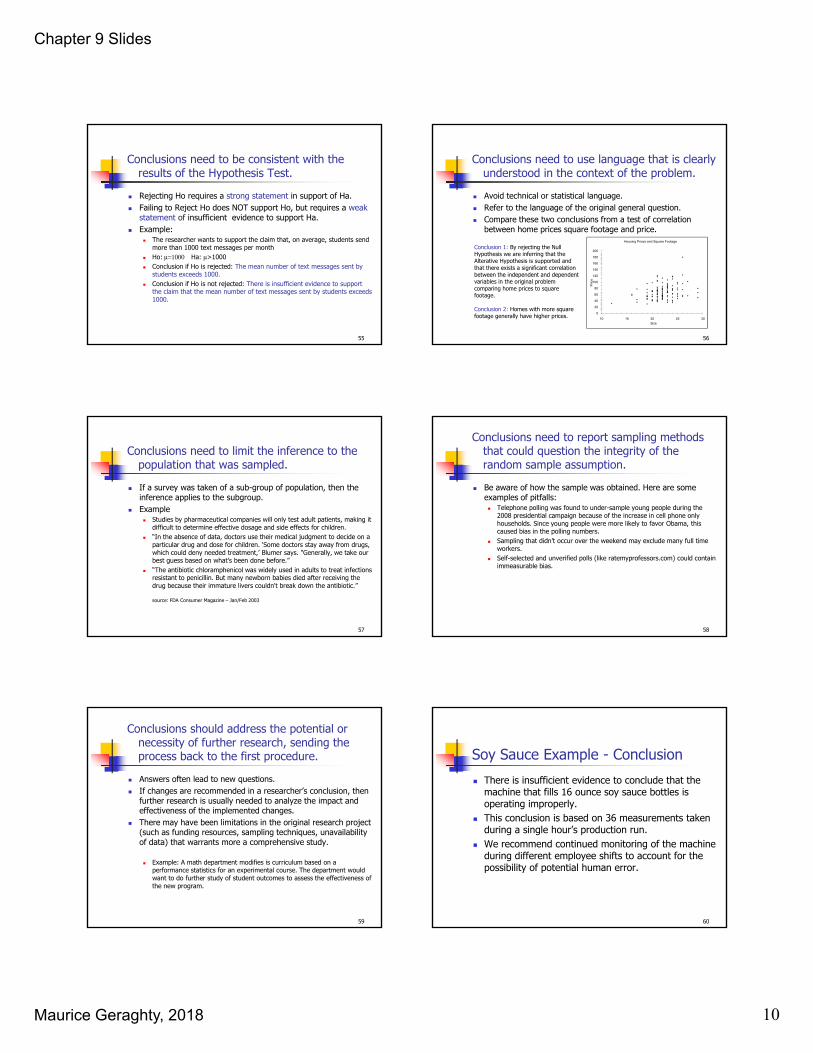
Conclusions need to use language that is clearly understood in the context of the problem.

Avoid technical or statistical language. Refer to the language of the original general question. Compare these two conclusions from a test of correlation

between home prices square footage and price.

56

0

20

40

60

80

100

120

140

160

180

200

10 15 20 25 30

Pric

e

Size

Housing Prices and Square Footage

Conclusion 1: By rejecting the Null Hypothesis we are inferring that the Alterative Hypothesis is supported and that there exists a significant correlation between the independent and dependent variables in the original problem comparing home prices to square footage.

Conclusion 2: Homes with more square footage generally have higher prices.

Conclusions need to limit the inference to the population that was sampled.

If a survey was taken of a sub-group of population, then the inference applies to the subgroup.

Example Studies by pharmaceutical companies will only test adult patients, making it

difficult to determine effective dosage and side effects for childrendifficult to determine effective dosage and side effects for children. “In the absence of data, doctors use their medical judgment to decide on a

particular drug and dose for children. ‘Some doctors stay away from drugs, which could deny needed treatment,’ Blumer says. "Generally, we take our best guess based on what's been done before.”

“The antibiotic chloramphenicol was widely used in adults to treat infections resistant to penicillin. But many newborn babies died after receiving the drug because their immature livers couldn't break down the antibiotic.”

source: FDA Consumer Magazine – Jan/Feb 2003

57

Conclusions need to report sampling methods that could question the integrity of the random sample assumption.

Be aware of how the sample was obtained. Here are some examples of pitfalls: Telephone polling was found to under-sample young people during the

2008 presidential campaign because of the increase in cell phone only households. Since young people were more likely to favor Obama, this y g p p y ,caused bias in the polling numbers.

Sampling that didn’t occur over the weekend may exclude many full time workers.

Self-selected and unverified polls (like ratemyprofessors.com) could contain immeasurable bias.

58

Conclusions should address the potential or necessity of further research, sending the process back to the first procedure.

Answers often lead to new questions. If changes are recommended in a researcher’s conclusion, then

further research is usually needed to analyze the impact and effectiveness of the implemented changes.

There may have been limitations in the original research project (such as funding resources, sampling techniques, unavailability of data) that warrants more a comprehensive study.

Example: A math department modifies is curriculum based on a performance statistics for an experimental course. The department would want to do further study of student outcomes to assess the effectiveness of the new program.

59

Soy Sauce Example - Conclusion There is insufficient evidence to conclude that the

machine that fills 16 ounce soy sauce bottles is operating improperly.

This conclusion is based on 36 measurements taken This conclusion is based on 36 measurements taken during a single hour’s production run.

We recommend continued monitoring of the machine during different employee shifts to account for the possibility of potential human error.

60

Chapter 9 Slides


Procedures of Hypotheses Testing

61



62





Statistical Power and Type II error

Fail to Reject Ho Reject Ho

63

Ho is true 1−αα

Type I error

Ho is False βType II error

1−βPower

Graph of “Four Outcomes”

64

Statistical Power (continued) Power is the probability of rejecting a

false Ho, when μ = μa Power depends on:

65

p Effect size |μo-μa| Choice of α Sample size Standard deviation Choice of statistical test

Statistical Power Example Bus brake pads are claimed to last on average

at least 60,000 miles and the company wants to test this claim.

66

The bus company considers a “practical” value for purposes of bus safety to be that the pads at least 58,000 miles.

If the standard deviation is 5,000 and the sample size is 50, find the Power of the test when the mean is really 58,000 miles. Assume α = .05

Chapter 9 Slides


Statistical Power Example Set up the test

Ho: μ >= 60,000 miles Ha: μ < 60,000 miles α = 5%

67

Determine the Critical Value Reject Ho if

Calculate β and Power β = 12% Power = 1 – β = 88%

837,58>X

Statistical Power Example

68

New Models, Similar Procedures The procedures outlined for the test of population

mean vs. hypothesized value with known population standard deviation will apply to other models as well.

Examples of some other one population models: Examples of some other one population models: Test of population mean vs. hypothesized value, population

standard deviation unknown. Test of population proportion vs. hypothesized value. Test of population standard deviation (or variance) vs.

hypothesized value.

69

Testing for the Population Mean: Population Standard Deviation Unknown

The test statistic for the one sample case is given by:

tX

=− μ

10-5

70

The degrees of freedom for the test is n-1. The shape of the t distribution is similar to the Z,

except the tails are fatter, so the logic of the decision rule is the same.

ts n

=/

Decision Rules

Like the normal distribution, the logic for one and two tail testing is the same.

For a two-tail test using the t-distribution, you will reject the null hypothesis when the value of the test statistic is greater than t or if it is less than - t

10-9

71

greater than tdf,α/2 or if it is less than - tdf,α/2

For a left-tail test using the t-distribution, you will reject the null hypothesis when the value of the test statistic is less than -tdf,α

For a right-tail test using the t-distribution, you will reject the null hypothesis when the value of the test statistic is greater than tdf,α

Example – one population test of mean, σ unknown

Humerus bones from the same species have approximately the same length-to-width ratios. When fossils of humerus bones are discovered, archaeologists can determine the species by examining this ratio. It is known that Species A has a mean ratio of 9.6. A similar Species B has a mean ratio of 9.1 and is often confused with Species A.

10-6

72

of 9.1 and is often confused with Species A. 21 humerus bones were unearthed in an area that was originally thought to

be inhabited Species A. (Assume all unearthed bones are from the same species.)

Design a hypotheses where the alternative claim would be the humerus bones were not from Species A.

Determine the power of this test if the bones actually came from Species B (assume a standard deviation of 0.7)

Conduct the test using at a 5% significance level and state overall conclusions.

Chapter 9 Slides


Example – Designing Test

Research Hypotheses Ho: The humerus bones are from Species A Ha: The humerus bones are not from Species A

In terms of the population mean

10-7

73

In terms of the population mean Ho: μ = 9.6 Ha: μ ≠ 9.6

Significance level α =.05

Test Statistic (Model) t-test of mean vs. hypothesized value.

Example - Power Analysis Information needed for Power Calculation

μo = 9.6 (Species A) μa = 9.1 (Species B) Effect Size =| μo - μa | = 0.5 σ = 0 7 (given)

74

σ = 0.7 (given) α = .05 n = 21 (sample size) Two tailed test

Results using online Power Calculator* Power =.8755 β = 1 - Power = .1245 If humerus bones are from Species B, test has an

87.55% chance of correctly rejecting Ho anda maximum Type II error of 12.55%

*source: Russ Lenth, University of Iowa – http://www.stat.uiowa.edu/~rlenth/Power/

Example – Power Analysis

75

Example – Output of Data Analysis

6 7 8 9 10 11 12

76

P-value = .0308α =.05Since p-value < αHo is rejected and we support Ha.

Example - Conclusions Results:

The evidence supports the claim (pvalue<.05) that the humerus bones are not from Species A.

Sampling Methodology: We are assuming since the bones were unearthed in the same location We are assuming since the bones were unearthed in the same location, they came from the same species.

Limitations: A small sample size limited the power of the test, which prevented us from

making a more definitive conclusion. Further Research

Test if the bone are from Species B or another unknown species. Test to see if bones are the same age to support the sampling

methodology.

77

Tests Concerning Proportion

Proportion: A fraction or percentage that indicates the part of the population or sample having a particular trait of interest.

9-24

78

The population proportion is denoted by .

The sample proportion is denoted by where

samplednumber sample in the successes ofnumber ˆ =p

p̂

p

Chapter 9 Slides


Test Statistic for Testing a Single Population Proportion If sample size is sufficiently large, has an

approximately normal distribution. This approximation is reasonable if np(1-p)>5

9-25

p̂

79

proportionsamplepproportionpopulationp

npp

ppz

ˆ

)1(ˆ

==

−−=

Example

In the past, 15% of the mail order solicitations for a certain charity resulted in a financial contribution.

A new solicitation letter has been drafted and will be sent to a random sample of potential donors.

9-26

80

A hypothesis test will be run to determine if the new letter is more effective.

Determine the sample size so that: The test can be run at the 5% significance level. If the letter has an 18% success rate, (an effect size of 3%), the power

of the test will be 95% After determining the sample size, conduct the test.


Research Hypotheses Ho: The new letter is not more effective. Ha: The new letter is more effective.

In terms of the population proportion

10-7

81

In terms of the population proportion Ho: p = 0.15 Ha: p > 0.15


Test Statistic (Model) Z-test of proportion vs. hypothesized value.

Example - Power Analysis

Information needed for Sample Size Calculation po = 0.15 (current letter) pa = 0.18 (potential new letter) Effect Size =| po - pa | = 0.03 Desired Power = 0 95

82

Desired Power = 0.95 α = .05 One tailed test

Results using online Power Calculator* Sample size = 1652 The charity should send out 1652 new solicitation

letters to potential donors and run the test.

*source: Russ Lenth, University of Iowa – http://www.stat.uiowa.edu/~rlenth/Power/

Example – Power Analysis

83

Example – Output of Data Analysis286

84

1366

Response No Response

P-value = .0042 α =0.05 Since p-value < α, Ho is rejected and we support Ha.

Chapter 9 Slides


EXAMPLECritical Value Alternative Method

Critical Value =1.645 (95th percentile of the Normal Distribution.)

H0 is rejected if Z > 1.645286

9-27

85

Test Statistic:

Since Z = 2.63 > 1.645, H0 is rejected. The new letter is more effective.

63.2

1652)85)(.15(.

15.1652286

=

−

=Z


The evidence supports the claim (pvalue<.01) that the new letter is more effective.

Sampling Methodology: The 1652 test letters were selected as a random sample from the charity’s The 1652 test letters were selected as a random sample from the charity s mailing list. All letters were sent at the same time period.

Limitations: The letters needed to be sent in a specific time period, so we were not able

to control for seasonal or economic factors. Further Research

Test both solicitation methods over the entire year to eliminate seasonal effects.

Send the old letter to another random sample to create a control group.

86

Test for Variance or Standard Deviation vs. Hypothesized Value We often want to make a claim about the variability, volatility or

consistency of a population random variable.

Hypothesized values for population variance σ2 or standard d i ti t t d ith th 2 di t ib ti

9-24

87

deviation σ are tested with the χ2 distribution.

Examples of Hypotheses: Ho: σ = 10 Ha: σ ≠ 10 Ho: σ2 = 100 Ha: σ2 > 100

The sample variance s2 is used in calculating the Test Statistic.

Test Statistic uses χ2 distribtion

s2 is the test statistic for the population variance. Its sampling distribution is a χ2 distribution with n-1 d.f.

88

0 1 0 2 0 3 0 4 0

2

22 )1(

o

snσ

χ −=

Example A state school administrator claims that the standard deviation

of test scores for 8th grade students who took a life-science assessment test is less than 30, meaning the results for the class show consistency. A dit t t t th t l i b l i 41 t d t An auditor wants to support that claim by analyzing 41 students recent test scores, shown here:

The test will be run at 1% significance level.

89


Research Hypotheses Ho: Standard deviation for test scores equals 30. Ha: Standard deviation for test scores is less than 30.

In terms of the population variance

10-7

90

In terms of the population variance Ho: σ2 = 900 Ha: σ2 < 900


Test Statistic (Model) χ2-test of variance vs. hypothesized value.

Chapter 9 Slides


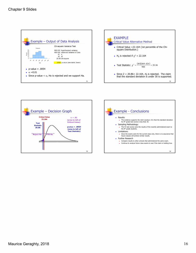
Example – Output of Data Analysis

10152025303540

Perc

ent

Histogram

91

p-value = .0054 α =0.01 Since p-value < α, Ho is rejected and we support Ha.

05

10

data

EXAMPLECritical Value Alternative Method

Critical Value =22.164 (1st percentile of the Chi-square Distribution.)

H0 is rejected if χ2 < 22.164

9-27

92

H0 is rejected if χ < 22.164

Test Statistic:

Since Z = 20.86< 22.164, H0 is rejected. The claim that the standard deviation is under 30 is supported.

( )( ) 86.20900

426.469402 ==χ

Example – Decision Graph

93


The evidence supports the claim (pvalue<.01) that the standard deviation for 8th grade test scores is less than 30.

Sampling Methodology: Th 41 t t th lt f th tl d i i t d t The 41 test scores were the results of the recently administered exam to the 8th grade students.

Limitations: Since the exams were for the current class only, there is no assurance that

future classes will achieve similar results. Further Research

Compare results to other schools that administered the same exam. Continue to analyze future class exams to see if the claim is holding true.

94

Documents

Chapter 9 Slidesnebula2.deanza.edu/~mo/Math10/ch09.pdf · Chapter 9 Slides Maurice Geraghty, 2018 6 Using Box Plot to find outliers The “box” is the region between the 1stand