Embed Size (px)
Citation preview
1
Chapter 9: Impacts of exurban development on water quality
Authors: Kathleen A. Lohse and Adina M. Merenlender
“Nothing is more fundamental to life than water. Not only is water a basic need, but adequate,
safe water underpins the nation’s health, economy, security, and ecology. The strategic challenge
for the future is to ensure adequate quantity and quality of water to meet human and ecological
needs in the face of growing competition among domestic, industrial-commercial, agricultural,
and environmental uses” (National Research Council 2004)
INTRODUCTION
Sustaining water resources has emerged as one of humanity’s greatest challenges
(National Research Council 2004); it requires managing existing threats to surface and ground
water quantity and quality as well as planning for future impacts due to changes in land use and
other global changes (Butcher 1999; Fitzhugh and Richter 2004). In many cases, however,
resource managers, conservationists, and planners have a limited understanding of the impacts of
human activities on stream and ground water conditions. In particular, little is known about how
different types of urban land use, especially low density housing development or exurban
growth, affect stream and groundwater conditions because tools to detect and quantify exurban
development, such as commonly used remotely sensed imagery (e.g., Landsat), cannot
adequately characterize differences in housing densities. Consequently, exurban development is
often excluded from model development and risk assessment. In addition, there is often large
2
uncertainty in how future type and extent of land use will impact these conditions. Together,
these factors make it challenging to predict how watersheds will respond to future changes and
other unforeseen interactions (Nilsson et al. 2003). In this chapter, we contend that despite these
large uncertainties, coupled land use impact--land-use change models can be important decision
support tools to identify areas that are more sensitive to land-use change, to examine the inherent
trade-offs associated with various policy options, and to identify options that result in water and
land conservation.
Agricultural and urban land use activities are often considered key drivers leading to
water quality impairment of streams and other water bodies (US EPA 2000). However, exurban
growth is increasingly recognized as an emerging development pattern in critical need of
ecological and water quality assessment (Theobald 2001; Theobald 2004). Indeed, exurban
development is the fastest-growing land-use type in the United States (US). (Heimlich and
Anderson 2001; Theobald 2003; Brown et al. 2005) and is expanding in Canada and Europe
(Dubost 1998; Azimer and Stone 2003). For example, recent nighttime aerial analyses of the
conterminous US have revealed that exurban development covers 14.3% of the US and
represents 37% of the population; urban areas make up 1.3% and represents 54.7% (Sutton et al.
2006). More importantly, urban and exurban development represent fundamental different types
of growth (Newburn and Berck 2006). Whereas urban development requires sewer and water
infrastructure before higher-density development (<1 acre/house) can be built, exurban
development (5-40 acres per house) is almost invariably serviced by private wells and septic
systems and, thus, not bound to existing or planned sewer and water service areas (SWSA).
These differences between urban and rural-residential development extend the possible range
and associated environmental impacts of rural-residential development such as sedimentation but

3
also temperature, organic wastewater contaminants and nutrient loading from septic systems well
beyond the urban fringe (Hansen et al. 2005; Newburn and Berck 2006; Lohse et al. 2008).
Together, differences in factors controlling urban and exurban development and their differential
land-use impacts indicate that planners and watershed managers will need to determine the
relative effects of exurban versus urban development. Land-use change models will also need to
distinguish between these different residential densities to forecast land-use development
patterns.
Coupling land-use impact models and land-use change models is emerging as a powerful
decision support tool for watershed manager and planners to help inform stakeholders about
inherent trade-offs associated with various land use and policy decisions as well as assist in
guiding conservation planning and development. Different scenarios can be generated from these
integrated models, and scenario planning can assist with environmental problem solving when
there is a high level of uncertainty about the system and manipulating the system is difficult
(Peterson et al. 2003). The difficulties inherent in integrating land-use impact models used by
hydrologists, geomorphologists, and ecologists, and models of land-use change used by planners
and economists are described by Nilsson et al. (2003). In brief, Nilsson et al. (2003) list a
number of improvements that need to be tackled by each discipline in order to develop useful
integrated models; until then, they argue that these disciplinary limitations will prevent the
development of useful integrated models for meaningful forecast relationships between future
expected land-use change and stream ecosystem responses. However, we believe that language
and epistemological barriers are rapidly being lowered by scientists who are increasingly cross-
trained in interdisciplinary environmental sciences. This new breed of scientists has the tools and
language to resolve many of the issues that have plagued earlier attempts at integrated modeling.

4
In particular, spatially explicit economic modeling is rapidly evolving to improve simulation
models of land-use change and consequent development patterns. Also, advances in land-cover
mapping via object recognition and high-resolution imagery, as well as a commitment on the part
of local governments to map cadastral data, have led to rapid improvements in source data for
land use and environmental modeling. So, while we acknowledge the need for continued
advances in each field to improve our disciplinary understanding, integrated models can be
developed that are useful to inform decision makers about inherent trade-offs associated with
various policy decisions and to identify future land-use and water management scenarios that are
more sustainable. With these limitations and goals in mind, we must follow the example set by
climate modelers and improve our modeled predictions, while explicitly addressing uncertainty
in resulting scenarios so as not to weaken our credibility with inaccurate predictions.
In this chapter, we present our current understanding of the impacts of different urban
land use types on water quality. We then outline how interactive decision-support tools or
models can be developed to minimize current and future land use impacts on water resources.
Essential steps in this model development process include: (1) quantifying relationships between
land use and water quality/quantity (land-use impacts), (2) developing land-use change scenarios
that forecast likely future land-use change scenarios, 3) developing economic valuation models,
and 4) integrating these models (land-use impacts, land-use change, and economic valuation) to
evaluate environmental and economic trade-offs (Figure 9.1). We use a case study to
demonstrate the utility of this approach to guide land-use planning that will ultimately improve
water quality and water security for human and natural systems. Our approach emphasizes that
parcel-level data can be used as the fundamental unit of land-use change to integrate and build
forecast models, resolve geographic resolution issues between models, and permit ecologists to
5
detect relative effects of low, medium and high-density housing as well as other land uses on
watershed processes.
REVIEW OF URBAN AND EXURBAN LAND-USE IMPACTS ON WATER QUALITY
Here we provide a brief review of the scientific literature focused on the impacts of
urbanization on water-quality characteristics including nutrients, organic pollutants, metals and
sedimentation. Conversion of land to exurban and urban housing development also alters
hydrology and these impacts are detailed in Chapter 11 of this volume. We focus this review on
differences in housing densities from exurban development (5-40 acres per house) to urban (<1
acres per house). In this chapter, we do not address a recent and growing trend in new
community developments in which developers build towns consisting of commercial, retail and
residential land uses outside of existing city boundaries because the development density is
similar to urban areas, and we expect the impacts of these new town developments will be
similar to urban development.
Water Quality Assessments and Sources
Assessments. States, U.S. territories, and other jurisdictions are required by Section 305b of the
Clean Water Act to assess the quality of the surface and groundwater and report their findings to
the US Environmental Protection Agency (EPA). Water bodies are then classified according to
water quality standards and their ability to meet designated uses, including aquatic life, fish
consumption, primary contact recreation, secondary contact recreation, drinking water supply,
and agricultural use. For example, surface or groundwater quality must not exceed the specified
Maximum Contaminant Level (MCL) established by the US EPA for each of the regulated water

6
quality constituents to meet drinking water standards. Similarly, surveys of sediments are
performed to estimate the probability of adverse effects of contaminated bed sediments on
aquatic and human life as required by the Water Resource Development Act of 1992. The
contaminant concentration in bed sediment that is expected to adversely impact benthic (or
bottom-dwelling) organisms has been specified as the Probable Effect Concentration (PEC).
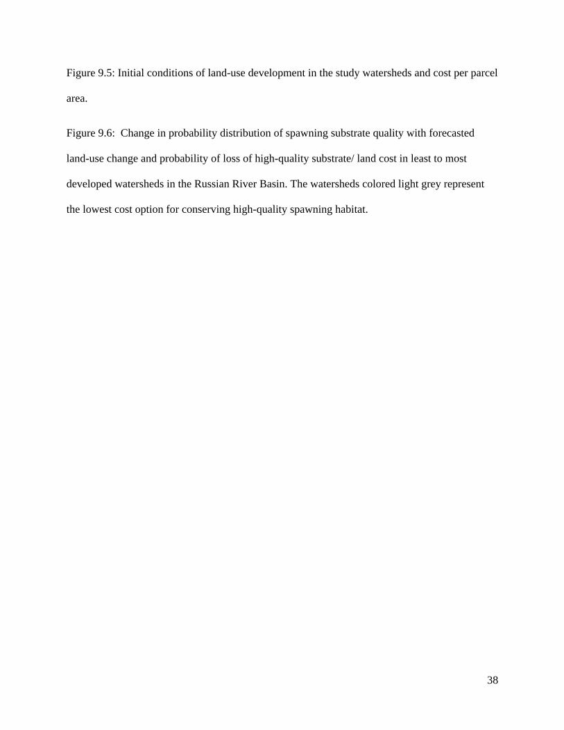
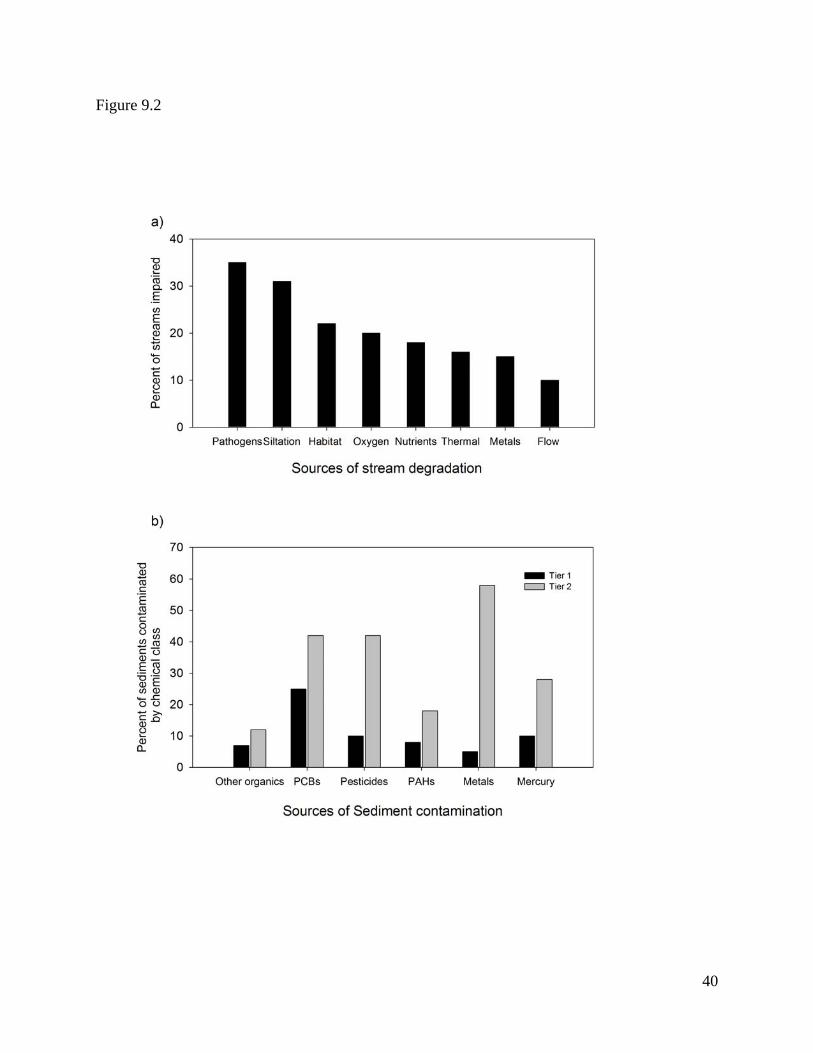
Based on these standards, the US EPA reported that 35,000 miles of river were impaired
by urban runoff and sewers in the US in the year 2000. An additional 28,000 miles were
impaired by municipal point sources, and 129,000 miles of river were impacted by agricultural
land use. Figure 9.2 shows that the leading source of impairment of rivers was pathogens
(bacteria) followed by siltation, nutrients and metals. Figure 9.2 also shows that of the surveyed
sediment (21,000 sites), 26% of the sediment samples were classified as Tier 1, indicating that
the observed contaminant concentrations were likely to have adverse effects on aquatic life and
possibly human health. Another 49% of the sites were classified as Tier 2 indicating possible, but
infrequently expected, adverse effects on aquatic ecosystems or human health. The most
frequently observed contaminants in Tier 1 were toxic organic compounds, specifically
polychlorinated biphenyls (PCBs) (20%), followed by pesticides, mercury (Hg) and then another
class of toxic organic compounds, polycyclic aromatic hydrocarbons (PAHs). Metals were the
most frequently encountered contaminant in Tier 2 (58%).
Sources. Sources of contaminants can be differentiated into point and non-point sources.
Point sources refer to discharge of contaminants from a specific location such as municipal
discharges from waste water treatment plants. Non-point sources are contaminants from more
diffuse sources and can be differentiated into atmospheric and fluvial sources. Atmospheric
deposition is commonly associated with organic pollutants such as PCBs and PAHs and metals

7
such as lead (Pb) and mercury (Hg) derived from coal combustion, burning of leaded gasoline
and other petroleum products. Non-point sources from watershed-derived fluvial transport
include runoff from agricultural fields, mine drainage, or urban areas such as pavement, lawns
and golf courses, and leaking septic tanks. In Table 9.1, we highlight sources of a select set of
contaminants and the predicted enrichment factor from conversion from rural to suburban to
urban land use. In the next sections, we examine in more detail the impacts of urbanization on
occurrence of different contaminants including organic compounds such as biological pathogens
and toxic organic compounds, inorganic compounds including nutrients and metals, and
sediments. We suggest best management practices to watershed managers, planners and
conservationists to minimize sources of contaminants in residential housing developments.
Organic contaminants
Organic contaminants include biological pathogens and other toxic organic substances.
Pathogens consist of a diverse group of bacteria, viruses, protozoa, and parasitic worms that are
responsible for many water-borne diseases such as gastroenteritis, malaria, river blindness
cholera, and typhoid fever (World Health Organization 2008). Although water-borne pathogen
associated fatalities remain low in the US owing to safe drinking water and sanitation practices,
water-borne diarrhoeal diseases (including cholera) claim 1.8 million lives each year, and
malaria claims 1.3 million lives each year in developing counties (World Health Organization
2008). Toxic organic substances include a plethora of human-derived compounds that vary in
weight, toxicity, and persistence in the environment (Miller and Miller 2007). Two common
classes of toxic organic groups known to pose a threat to human and ecosystem health include
polycyclic aromatic hydrocarbons (PAHs) and halogenated hydrocarbons (PCB), and these will
discussed in more detail below.
8
Biological pathogens. Biological pathogens, such as bacteria, protozoa, and viruses, have
emerged as primary stressors in surface waters (US EPA 2000) and have recently been found in
ground waters (Embrey and Runkle 2006). As mentioned above, the 2000 US EPA report
identified pathogens (bacteria) as the leading cause of degradation of rivers impairing
approximately 35% of the rivers assessed or 91,431 river miles (Figure 9.2). In a national survey
of ground water aquifers, Embrey and Runkle (2006) also showed high occurrence of coliform
bacteria; coliform were detected in 33% of the wells sampled. Rather than depth to well,
hydrogeologic characteristics and proximity to contaminated sources such as wastewater
treatment plants appeared to be more important predictors of occurrence of pathogens in
groundwater. These findings have raised awareness of the vulnerability of ground waters to
pathogens and the need to understand controls on transport of bacteria as well as viruses to
ground waters.
The impact of urbanization on pathogen sources, transport and fate is an area of active
research, and researchers are using different tools and techniques to address these questions (see
Field and Samadpour 2007 for a detailed review). Escherichia coli (E. coli) has been
increasingly used in monitoring studies as a reliable indicator of fecal contamination (Doyle and
Erickson 2006). However, the use of E. coli alone as an indicator organism has been questioned
because pathogens have been isolated from ecosystems where only low concentrations of fecal
coliforms exist (AWWA 1999; Field and Samadpour 2007). More studies are expanding to use
molecular techniques to develop microbial source tracking tools to identify the sources (e.g.,
human, domestic animal, wildlife, and/or bovine) and the pathogenic nature of the bacteria (Field
and Samadpour 2007).
9
To the knowledge of the authors, few studies have been published examining the impacts
of urbanization on the occurrence of fecal coliform. One of the few studies on this topic was
conducted in Georgia, US and showed that fecal coliform concentrations were significantly
higher during base and storm flow in urban watersheds compared to nonurban watersheds. In
these systems, fecal coliform typically exceeded EPA review criterion of 400 Most Probable
Number (MPN)/100 ml (Schoonover and Lockaby 2006). Land use impact models developed
from this work suggest fecal coliform will exceed EPA review criterion when development
exceeds 10 and 20% impervious surface cover. Additional studies are warranted in other
environmental settings to see if these patterns hold across different hydroclimates and to
understand the effects of transport versus source processes controlling the delivery of bacteria
and viruses to surface waters.
Until advances are made in terms of understanding the sources, transport, and fate of
bacteria, watershed managers and planners can follow best management practices to reduce
bacteria sources and delivery to streams. These practices include nonstructural and structural
methods. Specifically, nonstructural practices for low density residential development include
routine septic inspection and pump-outs and management of pet waste as well as manure from
domestic animals. For urban areas, management of pet waste and regular inspection of sewer
lines for leaks will reduce unexpected releases of feces into rivers and streams. Structural best
management practices include buffers, constructed wetlands, sand filters, infiltration trenches,
low impact development, and stream fencing. Examples of low impact development includes
permeable pavers, retention areas, grass swales, rain gardens, and minimizing impervious areas
to increase runoff infiltration, storage, filtering, evaporation, and onsite detention (public
communications, Low-Impact Development, www.EPA.gov/owow/nps/lid/). Although these

10
practices can help reduce bacteria in surface water, further studies are needed to evaluate the
effectiveness of these practices.
Halogenated hydrocarbons. Halogenated hydrocarbons are hydrocarbons that contain one or
more atoms of chloride (Cl), bromide (Br) or flouride (F) and are one of the largest and most
important groups of toxic organic contaminants. These chemicals have been linked to adverse
effects on aquatic and human health including cancer, reproductive problems, and nervous and
immune system problems (Miller and Miller 2007). Sources of halogenated hydrocarbons
include solvents, cleansers, and degreasers but also pesticides, electrical equipment, and
commercial products. Examples of halogenated hydrocarbon solvents are trichloroethylene
(TCE) and chloroform. Prominent examples of halogenated hydrocarbon pesticides are Dichloro-
Diphenyl-Trichloroethane (DDT) and 2,4-Dichlorophenoxyacetic acid (2, 4-D). Polychlorinated
biphenyls (PCBs) are also chlorinated hydrocarbons often used in electrical equipment. Although
polychlorinated biphenyls (PCBs) have been banned in the U.S. since the 1970’s, high levels of
PCBs can still be found in river and lake sediments owing to their continued use in equipment
made with PCBs, their slow degradation rate, and persistence in the environment (Miller and
Miller 2007). Dichloro-Diphenyl-Trichloroethane (DDTs) were also banned in the 70’s and take
a long time to break down, tend to accumulate, and bio-magnify in biota. The persistence of
these chemicals was highlighted in a recent national survey of surface waters and ground waters
(1992-2001) showing banned (DDT, PBC) and newer organochlorine compounds (chlordane,
dieldrin) detected in fish and bed sediments in most streams in the US (Gilliom et al. 2007). In
addition, at least one type of pesticide was detected in 90% of the surveyed streams and in 50%
of the groundwater wells (Gilliom 2007; Gilliom et al. 2007)

11
The few studies evaluating relationships between increasing urban intensification (i.e. the
conversion from rural to suburban to urban) and particle-associated and water-associated
halogenated organic compounds have shown that concentrations of halogenated hydrocarbons
increase with the percentage of commercial, industrial, and transportation land use (CIT) in a
watershed. Along a rural to urban gradient in the Northeast US, for example, Chalmers et al.
(2007) showed higher concentrations of halogenated hydrocarbons in sediments in areas with
higher percentage of CIT land use. Land use impact models generated from this work suggest
conversion from rural to suburban will result in 2 fold increase in DDT and PCBs and suburban
conversion to urban will result in a 3-4 fold increase (Figure 9.3) (Chalmers et al. 2007). Despite
the high occurrence of chlorinated hydrocarbons in stream sediments, surveys of urban and
reference lake sediment cores (using lakes as long-term historical records of deposition of
compounds) show that concentrations of DDT and PCBs in sediment cores are declining over
time across the US, suggesting that sources of DDT and PCB in the environment are generally
decreasing as these chemicals are being phased out of use and eventually degraded (Van Metre et
al. 1997; Van Metre et al. 1998; Van Metre and Mahler 2005). Nonetheless, these studies
highlight the persistence of halogenated hydrocarbons in the environment; once released in the
environment, these compounds persist for decades to centuries.
Occurrence of other halogenated hydrocarbons such as pesticides and herbicides in
surface and shallow ground waters is also high in urban to undeveloped areas. In an USGS study,
pesticides were detected in 97% of the surface water and 55% of the ground waters sampled in
urban areas (Gilliom et al. 2007). Surprisingly, the study also detected pesticides in 65% of
surface waters and 29% of ground waters in undeveloped watersheds. In addition, more than half
the fish sampled in undeveloped watersheds contained organochlorines indicating deposition and

12
persistence of these compounds in the environment. In another study across six metropolitan
areas, Sprague and Nowell (2008) showed that insecticide concentrations increased significantly
with increasing urban cover in low flow conditions whereas herbicides increased with increasing
urban cover in three out of the cities examined (Sprague and Nowell 2008). Large agricultural
influences in the other three cities appeared to explain herbicide patterns in stream flow.
Best management practices for reducing halogenated hydrocarbons in urbanizing areas
include nonstructural and structural practices. Examples of structural practices include reducing
halogenated hydrocarbon pesticides and insecticides or using non-halogenated hydrocarbon
pesticide and insecticides. Inspection of older electrical equipment and phasing out of older
and/or leaking equipment that may contain PCBs is also advised. Structural practices include
LID methods and others described in the biological pathogen subsection.
Polycyclic aromatic hydrocarbons. In contrast to PCBs and DDTs that appear to be
declining over time, polycyclic aromatic hydrocarbons (PAHs) are on the rise (Van Metre and
Mahler 2005). Polycyclic aromatic hydrocarbons originate from natural and anthropogenic
combustion of organic material, including fossil-fuel burning in automobiles, power plants, and
heating facilities, and have been identified as potentially carcinogenic. They can also be found in
creosote, roofing tar and asphalt sealant (Mahler et al. 2005). Indeed, coal-tar-emulsion based
and asphalt-emulsion based sealcoats have been recently identified as large sources of PAHs.
These sealants are used by many homeowners and commercially and applied to parking lots
associated with commercial businesses, apartments, condominium complexes, churches, schools,
and business parks, and residential driveways. A study by Mahler et al. (2005) found much
higher PAHs in runoff from parking lots sealed with coal-tar based sealcoat compared to those
sealed with asphalt-based sealant; the average PAH concentrations in particles in runoff from

13
coal-tar sealed parking lots was 3,500 mg/kg or 65 times higher than concentrations in particles
from parking lots not seal coated (54 mg/kg). Average concentrations in particles from asphalt-
based sealcoat were lower, 620 mg/kg. The concentration of total PAHs likely to adversely affect
aquatic organisms, or the PEC, is 22.8 mg/kg (Mahler et al. 2005). Together, these findings
suggest new development and associated vehicular traffic and driveway sealants are major
source of PAHs to streams.
Because PAHs are produced as byproducts from partial combustion of fossil fuels and
other products, several studies have examined atmospheric transport distances of PAHs and also
PCBs. In general, polycyclic aromatic hydrocarbons and PCB’s tend to decline with distance
from urban areas due to lower emission rates. However, persistent gas-phase PAHs, often
alkylated PAHs, increase from urban to rural locations (Gingrich and Diamond 2001). These
persistent gas phase compounds can travel as far as 50 km, whereas more reactive gas-phase and
particle-phase compounds often travel shorter distances, <5 km (Gingrich and Diamond 2001).
The impacts of atmospheric transport of PAHs can be seen at the urban fringe, in areas that are
undergoing rapid urban spawl, where rapid increases in PAHs in lake sediments have been
linked to increased automobile use for commuting (Van Metre et al. 2000). These findings
suggest that urban sprawl may adversely impact water quality within a watershed due to large
increases in traffic to and from urban centers.
Like PBCs and DDTs, polycyclic aromatic hydrocarbons have also been strongly
correlated to the percent of commercial, industrial and transportation (CIT) land use in a
watershed (Figure 9.3). Based on their land use impact model from the Northeast US, Chalmers
et al. (2007) predict that PAHs will increase by a factor of 6 when a rural site becomes suburban
and increase by a factor of 5 when the suburban sites becomes urban. Their model also predicts
14
that the PEC for PAHs will be exceeded at 13% CIT. Research in other regions of the US is
warranted but this study provides evidence for upward trends in PAHs with land use
intensification. Based on these findings and the upward trend in PAHs in urban lake sediment
cores relative to reference lakes (Van Metre and Mahler 2005), it is expected that PAHs will
likely to surpass chlorinated hydrocarbons as a threat to human health and aquatic biota in
streams and lakes in the coming decades.
Polycyclic aromatic hydrocarbons are emerging as threats to human and aquatic health,
and the sources of PAHs include atmospheric deposition from incomplete combustion of fossil
fuels as well as watershed sources such as asphalt sealants. Reducing atmospheric sources of
PAHs such as vehicular traffic remains challenging and will require transportation alternatives
and stricter zoning controls on urban sprawl. On the ground, planners, watershed managers,
developers, and individual homeowners can apply best management practices to reduce
watershed sources of PAHs by reducing or eliminating driveway sealants and/or finding
alternative sealants. Structural practices described above can also reduce delivery of PAHs to
streams.
Other organic compounds. Many organic compounds such as pharmaceutical, hormones, and
other organic wastewater compounds are not currently regulated by the US EPA and cannot be
readily removed by wastewater treatment or septic systems. A recent national survey of 139 US
streams revealed that organic contaminants including pharmaceutical, hormones, and other
organic wastewater compound (OWC) were detected in 80% of the rivers sampled (Kolpin et al.
2002). Most frequently detected compounds included coprostanol (fecal steroid), cholesterol
(plant and animal steroid), N,N-diethyltoluamide (insect repellant), caffeine (stimulant), triclosan
(antimicrobial disinfectant), tri(2-chloroethyl)phosphate (fire retardant), and 4-nonylphenol

15
(nonionic detergent metabolite) (Kolpin et al. 2002). The impact of these individual compounds
and the interaction of them on aquatic and human health remain unclear. Further research is
warranted to understand the aquatic and human health risks of these compounds.
Nutrients
Nutrient concentrations have increased in rivers throughout the US and the world
(Howarth et al. 1996; Mueller and Spahr 2006). Non-point sources of nitrogen (N) and
phosphorus (P) dominate surface waters (Howarth et al. 1996; Carpenter et al. 1998; Caraco and
Cole 1999) and are highly correlated with population density and net anthropogenic inputs to the
watersheds. Dominant sources of nitrogen (N) to watersheds include fertilizers, atmospheric N
deposition, food and animal feed imports, and biological N fixation in leguminous crops.
Because P and sometimes N can limit productivity of surface waters, one of the main impacts of
nutrients is through the process of eutrophication whereby lakes, reservoirs and sometimes rivers
have excess algal or plant growth leading to degradation of water bodies. High levels of nitrate
(>10 mg/L nitrate-N) in surface and ground waters can also have human health consequences,
interfering with the ability of the blood to carry oxygen, particularly in infants.
A growing body of research indicates that nutrient concentrations and loads in rivers
increase as development increases. In a national survey of streams and rivers, Mueller and Spahr
(2006) showed concentrations of all nutrients (total nitrogen, total phosphorus, nitrate,
orthophosphate) were significantly greater in partially developed watersheds than ing
undeveloped watershed but significantly less than more developed agricultural, urban, and mixed
land-use watersheds. Other studies have shown similar patterns at smaller spatial scales
(Groffman et al. 2004; Lewis and Grimm 2007). The impact of exurban development on nutrient
16
loading to rivers is most apparent in mountainous headwater catchments undergoing rapid
development, such as those in Colorado. In these systems, exurban development has been linked
to increases in dissolved inorganic nitrogen in streams during spring melt; 19-23% of this
nitrogen is estimated to be coming from septic systems (Kaushal et al. 2006). Increased nitrate
export from these headwater catchments indicates that the biotic capacity of these headwater
catchments to take up this N is very limited, indicating these systems are more sensitive to
development than other systems. Kaushal et al. (2006) suggest that because much of the world’s
population relies on water originating from mountain areas, even modest levels of nutrient
enrichment can result in cascading effects on water supplies downstream.
Metals
Trace metals are metals found in very low concentrations in nature, and include arsenic
(As), silver (Ag), cadmium (Cd), chromium (Cr), copper (Cu), mercury (Hg), iron (Fe),
manganese (Mn), nickel (Ni), lead (Pb), zinc (Zn) and others. Several of these metals are
essential for plant and animal life at low concentrations but become toxic at higher
concentrations (Miller and Miller 2007). Trace metals can enter terrestrial and aquatic
ecosystems by atmospheric deposition and point and non-point sources. Atmospheric deposition
is an important source of trace metals, particularly for Hg and Pb. Indeed, some studies suggest
that nearly all the Hg in water, sediment and fish can be explained by atmospheric deposition
(Sorensen et al. 1990). Point and non-point sources of trace metals include mining byproducts,
chemical waste, coal and industrial waste, metal plating, and plumbing.
Like organic compounds and nutrients, trace metals are highly correlated with population
density and percent commercial, industrial, and transportation land use (CIT) (Figure 9.3). For
17
example, the sum of trace elements (Cu, Pb, Hg, Zn) in streambed sediments is highly correlated
with population density (Rice 1999), and anthropogenic Pb and Zn concentrations can be
accurately predicted by population density (Callender and Rice 2000). However, spatial
distribution of Pb and Zn depends on time of development; removal of leaded gasoline in the late
1970’s has led to declines in lead and increased vehicular usage has kept Zn concentrations high
in runoff and sediments. Consistent with these spatial observations, declines in lead have been
observed in long-term lake sediment records, whereas high Zn concentrations have been
observed in recent exurban developments because of high vehicular traffic (Mahler and Van
Metre 2006). Work by Chalmers et al. (2007) suggests that metal concentrations will double
when a rural site becomes suburban and again triple when the suburban site becomes urban
(Table 9.1, Figure 9.3). Finally, concentrations of metals are predicted to exceed PEC standards
between 3% CIT for Pb and 10-25% CIT for Zn, Hg, Cu, and Cd. Best management practices for
metals include reducing source of metals by reducing vehicular use and traffic. Elimination or
use of alternative chemicals for timber treatment and preservation that do not contain metals will
also reduce metals in watersheds. In addition, structural practices to reduce delivery of metals to
streams can be implemented including, but are not limited to, LID methods. Finally, more
transformative planning options to reduce metals in watersheds include transferring development
rights in undeveloped watersheds to more developed watersheds that are already likely to be
already impacted by metals and other contaminants.
Sedimentation
Numerous studies have linked in-stream sediment conditions to upland landscape
components and land-use change in watersheds (e.g. Richards et al. 1996; Wohl and Carline
1996; Sutherland et al. 2002; Opperman et al. 2005). Agricultural and urban land use activities
18
are often considered the key drivers increasing fine sediment production and delivery to streams
(Waters 1995; Pimentel and Kounang 1998). Compared to land with native vegetation,
agriculture can result in significantly higher rates of sediment production, even on moderate
slopes, due to the increased amount of bare soil exposed to the erosive power of raindrops and
sheet wash (Dunne and Leopold 1978; Chang et al. 1982; Pimentel and Kounang 1998) and
indirectly due to higher rates of runoff that lead to increased incision and bank erosion (Chang et
al. 1982). Urban areas produce large amounts of fine sediment during periods of construction and
can continue to produce sediment over longer time periods from bank erosion (Trimble 1997;
Pizzuto et al. 2000). Less is known, however, about the impacts of exurban development and the
relative impacts of different land uses on sediment production and delivery to streams; this issue
is the focus of the watershed-scale case study described below.
A summary of a limited set of studies examining the impact of different urban land use
types on water quality indicate that the process of urbanization dramatically increases the
occurrence of organic pollutants as well as nutrients, metals, and sediments in streams (Table
9.1). In most cases, conversion of rural areas to suburban development is predicted to double the
concentration of contaminants, with the exception of PAHs that is predicted to increase by 6
fold. Conversion of suburban to urban is predicted to result in a 3 to 5 fold increase in
contaminants. Based on Chalmers et al. (2007) study, once the percentage of commercial,
industrial and transportation land use exceeds 15%, contaminants in sediments will likely exceed
the Probable Effect Concentration (PEC) and adversely impact aquatic and possibly human
health. Further studies are warranted in other regions of the US to evaluate these relationships,
and several studies are ongoing in the rapidly urbanizing desert Southwest in Tucson and also
Phoenix. However, the study by Chalmers et al. (2007) suggests that the process of urbanization,
19
the conversion of undeveloped land to suburban and ultimately to urban land uses, dramatically
increases the occurrence of organic pollutants, nutrients, and metals in the environment and
reduces water and sediment quality.
To reduce these contaminants, planners and watershed managers should implement best
management practices. One the most effective means to reduce these contaminants in watersheds
is to eliminate use or not introduce these contaminants in the first place. For example, developers
and homeowners can potentially eliminate PAH-containing driveway sealants and advocate for
PAH-free alternatives. Structural practices can help to reduce the delivery of contaminants to
streams once they are introduced into the environment. Finally, there are more transformative
planning options available to planners, conservationists, and watershed managers. One of these
options, which we describe below in detail, involves the development of coupled land-use
impact-land use change models and use of Transfer of Development Rights (TDR) to protect
sensitive land by transferring the "rights to develop" from one area and giving them to another.
ASSESSMENT OF RELATIVE LAND-USE IMPACTS AND APPLICATION OF
COUPLED ENVIRONMENTAL -ECONOMIC LAND-USE CHANGE MODEL TO
WATERSHED PLANNING: A CASE STUDY FROM THE RUSSIAN RIVER BASIN,
CALIFORNIA
Overview of Coupled Environmental-Economic Land Use Change Model
We draw on our research from the Russian River Basin in Sonoma County, California to
demonstrate how the steps outlined in Table 9.2 are used to develop the necessary models needed
to project changes in water quality with future land use change (Figure 9.1). Specifically, we
20
analyzed the relative impacts of three different land uses (urban, exurban, and vineyard
development) on levels of fine sediment in streams (Lohse et al. 2008). Fine sediment is one
measure of water quality that reduces habitat suitability for spawning salmonids, and data on
levels of fine sediment or embeddedness were available throughout much of the Russian River
basin from the California Department of Fish and Game. We used these data to quantify the
impacts from urban and agriculture on elevated levels of fine sediment in streams, as well as
determine the extent to which exurban development impacts water quality (Step 1). We then
developed an economic land use change model (Step 2) and land price valuation model (Step 3).
Because all of our models utilized parcel-level data, we could distinguish among low, medium,
and high-density housing, detect relative effects of these different types of housing as well as
other land uses on watershed processes, resolve geographic resolution issues between models,
and couple these models to forecast expected loss of water quality and assess the risk of land-use
conversion at a watershed scale (Step 4). Finally, we could compare these expected losses in
water quality to the cost of preventing these impacts through upland conservation. This case
study provides an important demonstration of how coupling environmental, land-use, and
economic modeling can provide a useful tool to forecast scenarios that examine environmental
and economic trade-offs and can help guide land-use planning for conserving and restoring water
resources.
Step 1: Environmental Data for Land-Use Impact Model
The first step of our integrated modeling approach was to develop an empirical land-use
impact model using land-use classification data at the parcel-level scale and water quality on
levels of fine sediment from low (1) to high (4) for each sampled stream reach. We classified
land use using parcel data from the county assessor’s office to provide more accurate residential

21
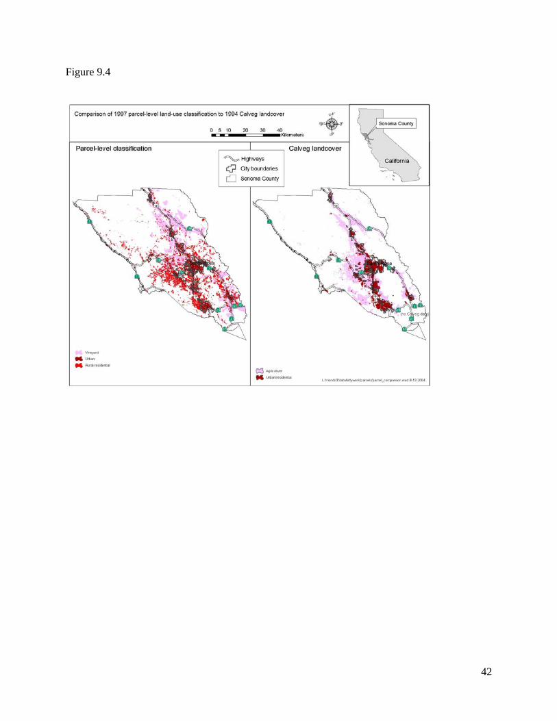
classification than LANDSAT TM imagery. A comparison of land-use classification by parcel-
level data and LANDSAT TM imagery in Figure 9.4 shows how much better the former source
data is for mapping exurban development. In our case, the 1997 Sonoma County tax-assessment
data contained the number of residential structures, year built, lot size, and other land-use
characteristics for each parcel. We distinguished between urban (<1 acre per structure) and rural-
residential (1-40 acres per structure) because a housing density of 1 acre per structure is the
typical limit on residential development serviced by septic systems (Newburn and Berck 2006).
Intensive agriculture in these watersheds was almost exclusively wine grape growing. Parcels
were classified as vineyard if the parcel had at least 10% vineyard or at least 5 hectares of
vineyard based on digital maps derived from aerial photographs.
We then used ordinal logistic statistical modeling techniques to develop response models
relating the rank level of fine sediment at each salmonoid spawning site with land-use and other
independent variables (see Hosmer and Lemeshow 2000 for details on model development). The
field data on fine sediment levels was included from 93 watershed reaches with an average of 54
spawning sites per reach. To examine the relationship between land use and level of fine
sediments surrounding spawning gravels, as a measure of spawning-habitat quality, we used a
10-m Digital Elevation Model in a Geographic Information System (GIS) to delineate
watersheds above the downstream end of all the surveyed reaches that met several sampling
criteria. Explanatory variables included existing aerial percentages of vineyard, urban, and rural-
residential land use in 1997 within each upstream watershed. Biophysical watershed variables
such as road density, a stream power index, a hillslope stability index as well as categorical
variables including channel type, dominant geology, and river bank-substrate material (bedrock,
boulder, silt/clay, cobble) were also included.

22
The results of the ordinal logistic model showed fine sediment levels decreased with
increasing percentage of three land-use types (urban, exurban and vineyard) in watersheds, with
urban development having a larger marginal impact than either rural-residential or vineyard use
(Lohse et al. 2008). To explore the relative importance of including exurban development in our
model, rather than just urban development as is done in most models, we compared statistical
models with and without exurban land-use. We found our predictions of fine-sediment were
better when the amount of exurban development was included. To examine the robustness of the
model, we performed a goodness of fit test in which we included an additional data set of
watersheds in the statistical model that were not used for model building. The coefficients in the
model were not significantly altered by this additional data set suggesting a robust model fit.
Step 2: Land use change modeling
The next step of the process was the construction of a land-use change model using parcel
data for the period 1994-2002 using the parcel-level land-use data described above. Land-use
conversion was defined as any transition from developable parcel into vineyard, urban or
exurban development during the period 1994–2002. A multinomial logit model, a statistical
model that predicts the probability of an event occurrence by fitting categorical and/or numerical
data to a logistic curve, was developed to explain land-use transitions as a function of parcel-site
characteristics, including average slope, growing degree days (microclimate), 100–year
floodplain, proximity to major employment centers, designated sewer and water services
(SWSA), and minimum lot-size zoning.
The estimated coefficients from the multinomial logistic regression were used to predict
the site-specific conversion probabilities for each developable parcel based on mapped site

23
characteristics. Then we used the land-use change model to simulate the estimated future amount
and location of development for each land-use type within each watershed. During this build-out
step, each parcel could remain developable or become converted to one of the five developed
land-use types in a given simulation according to the site-specific conversion probabilities. To
map the forecasted future pattern of land use, we added the amount of estimated land-use change
to the actual extent of land-use type already mapped. Our future development scenarios spanned
2002–2010 because the land-use change model was based on development over an eight year
period (1994–2002). In our case, we forecasted the amount of land-use change under a
“business-as-usual” scenario; however, other scenarios including changes in land-use policies
could be run as well.
Step 3: Economic Valuation Model
To examine the economic tradeoffs along with expected changes to water quality, we
employed an existing parcel-level land valuation model. The estimated land values were derived
from a hedonic price model that uses recent property transactions to estimate the market value of
developable land as a function of site-specific characteristics (Newburn et al. 2006). Tax
Assessor data provided the necessary information on individual parcels for the land value,
current land use, and other property characteristics. We then used a similar set of explanatory
variables for each parcel, including characteristics for land quality (slope, elevation,
microclimate, 100-year floodplain), accessibility (travel times to urban centers, sewer and water
service), neighboring land-use externalities (percent protected open space and urban), and zoning
(land use designations, minimum lot size) to build a spatially explicit economic land valuation
model. For each developable parcel, we were then able to estimate the value of developable land
because key site characteristics were known within the GIS. As shown in Figure 9.5, the

24
predicted value of developable land was observed to range over several orders of magnitude. The
large degree of variation in land prices highlights why priority setting for land conservation
should include the spatial heterogeneity in land values (Figure 9.5).
Step 4: Environmental- economic decision support tool
The final step of coupling the land-use impact model and economic land use change
model involved forecasting the probability distribution of fine sediment levels based on the
expected percentages of each land-use type in 2010 and the estimated parameters in the
ordinal logistic model. In our case study, we found that forecasted rural-residential and
vineyard development had much larger influences on decreasing water quality than urban
development. This is because the land-use change model estimated 10 times greater land-use
conversion to both rural-residential and vineyard compared to urban. Also, forecasted urban
development was concentrated in the most developed watersheds, which already had poor
spawning substrate quality, such that the marginal response to future urban development was
less significant.
A land conservation targeting rule was used to identify priority areas for protection based
on the expected loss of water quality due to future land-use conversion and the average land
costs in each watershed. In our case, we maximized conservation goals based on the objective of
minimizing the expected loss in environmental benefit per unit cost (Newburn et al. 2006).
Applying this targeting rule to our results, we identified priority areas by summing the relative
probabilities of loss of high quality sites (levels 1 and 2) and dividing by the average cost per
acre for that watershed (Figure 9.6). Figure 9.6 shows the initial level of development in the
watersheds and the change in water quality with future land use change. Findings from our study
25
suggested that conservation efforts should target moderately and less-developed watersheds to
meet the goal of protecting water quality for salmonid-spawning habitat, where future rural-
residential development and vineyards threaten high-quality fish habitat, rather than the most-
developed watersheds, where land prices typically are much higher and land-use development,
particularly urban development, has already resulted in significant habitat degradation (Figure
9.5). With this decision support tool and spatial maps of environmentally sensitive watersheds at
risk to future development, decision-makers can work to influence the density and location of
future residential development through local zoning and other land-use policies. In particular, we
recommended that a Transfer of Development Rights (TDR) program be implemented to curtail
lower-density rural-residential development within moderate- and less-developed watersheds
(sending areas in light grey, Figure 9.6), while encouraging higher-density infill urban
development to take place in areas already highly disturbed (receiving areas in dark grey
watersheds, Figure 9.6). Finally, in concert with these more transformative planning tools,
effective runoff and construction control techniques, best management practices for road
construction and maintenance (public communications, Roads, Highways, Bridges-NPS
categories, http://www.epa.gov/owow/nps/roadshwys.html), and other low impact development
(LID) strategies (public communications, Low-Impact Development,
www.EPA.gov/owow/nps/lid/) can be used at a local scale when development does occur in
sensitive watersheds.
CONCLUSIONS

26
In this chapter, we examined the impacts of urbanization on water quality, with particular
emphasis on the expansion of housing development beyond the urban fringe. A review of the
literature indicates that conversion from rural to suburban increases the occurrence of organic
pollutants, as well as nutrients, metals, and sediments in streams, with potentially adverse effects
for stream biota and humans. The main drivers behind these patterns appear to be increased
population density, increased roads and hence increased vehicular traffic that results in
deposition and fluvial transport of metals and organic pollutants to streams and sediments.
Exurban development and associated roads also extend possible land-use impacts by increasing
nutrient and fecal bacteria inputs to streams through leaking septic systems and increased
vehicular traffic, both of which result in increased nitrogen inputs to watersheds.
We used a case study from the Russian River Basin in California to illustrate how to
couple water-quality modeling and land-use change models to guide conservation planning and
development. In this case study, we developed a land-use impact model to predict the relative
impacts of urban and exurban development on sedimentation in streams that support rare
salmonids. We then coupled this model with a land-use change model to predict where
conversion to exurban and urban development would take place (Figure 9.6). With both models,
we differentiated between exurban and urban because they represent different types of growth,
and we showed that they have differential impacts on substrate quality in streams. We showed
that exurban development has a larger potentially impact on water quality because of its ability
to “leapfrog” into previously undeveloped areas, a finding that is likely to transfer to different
environmental settings.
The case study presented here demonstrates that land-use impact modeling can be
coupled with land-use change and economic modeling to forecast scenarios of future ecological
27
conditions and therefore guide land-use and restoration planning. Although we are unable to
generate highly accurate predictions, we need to examine the inherent trade-offs associated with
various policy options to (1) better inform local decision-makers about trade-offs and (2) identify
options that result in water and land conservation. The importance of scenario planning and
engaging communities in this process is widely recognized (Hopkins and Zapata 2007), and we
argue that our ability to integrate conservation planning with land-use planning hinges on our
ability to develop useful future scenarios. Given that there are always multiple ecosystem
services traded-off for any proposed ecosystem alteration, it is critical that scenarios be
developed that take uncertainty into account and reduce the changes for unintended
consequences or perverse results. We conclude that coupled environmental impact-land use
change models provide an adaptive-management tool to manage existing threats to surface and
ground water quantity and quality as well as plan for future impacts owing to changes in land
use.
ACKNOWLEDGMENTS
We thank Shane Feirer for assistance on GIS maps and Dave Newburn for his contributions to
the Russian River case study and land-use change modeling.
REFERENCES
AWWA. 1999. Manual of Water Supply Practices – M48: Waterborne Pathogens., American
Water Works Association, Denver, CO.

28
Azimer, J., and L. Stone. 2003. The Rural West: Diversity and Dilemma. Canada West
Foundation, Calgary, Alberta.
Brown, D. G., K. M. Johnson, T. R. Loveland, and D. M. Theobald. 2005. Rural land-use trends
in the conterminous United States, 1950-2000. Ecological Applications 15:1851-1863.
Butcher, J. B. 1999. Forecasting future land use for watershed assessment. Journal of the
American Water Resource Association 35:555-565.
Callender, E., and K. C. Rice. 2000. The urban environmental gradient: anthropogenic influences
on the spatial and temporal distribution of lead and zinc in sediments. Environmental
Science and Technology 31:424a-428a.
Caraco, N. F., and J. J. Cole. 1999. Human impact on nitrate export: An analysis using major
world rivers. Ambio 28:167-170.
Carpenter, S. R., N. F. Caraco, D. L. Correll, R. W. Howarth, A. N. Sharpley, and V. H. Smith.
1998. Nonpoint pollution of surface waters with phosphorus and nitrogen. Ecological
Applications 8:559-568.
Chalmers, A. T., P. C. Van Metre, and E. Callender. 2007. The chemical response of particle-
associated contaminants in aquatic sediments to urbanization in New England, U.S.A.
Contaminant Hydrology 91:4-25.
Chang, M., F. A. Roth, and E. V. Hunt, editors. 1982. Sediment production under various forest-
site conditions. International Assocation of Hydrological Sciences, Wallingford, UK.
Doyle, M. P., and M. C. Erickson. 2006. Closing the door on the fecal coliform assay. Microbe
1:162-163.
Dubost, F. 1998. De la maison de campagne à la résidence secondaire. Pages 10-37 in F. Dubost,
editor. L’autre maison: la ‘résidence secondaire’, refuge des générations. Éditions, Paris.

29
Dunne, T., and L. B. Leopold. 1978. Water in Environmental Planning. W. H. Freeman, New
York, New York, USA.
Embrey, S. S., and D. L. Runkle. 2006. Microbial quality of the Nation’s ground-water
resources, 1993–2004. US Geological Survey Report 2006-5290.
Field, K. G., and M. Samadpour. 2007. Fecal source tracking, the indicator paradigm, and
managing water quality. Water Research 41:3517-3538.
Fitzhugh, T. W., and B. D. Richter. 2004. Quenching urban thirst: growing cities and their
impacts on freshwater ecosystems. Bioscience 54:741–754.
Gilliom, R. J. 2007. Pesticides in the Nation's Streams and Ground Water. Environmental
Science and Technology 41:3408-3414.
Gilliom, R. J., J. E. Barbash, C. G. Crawford, P. A. Hamilton, J. D. Martin, N. Nakagaki, L. H.
Nowell, J. C. Scott, P. E. Stackelberg, G. P. Thelin, and D. M. Wolock. 2007. The
Quality of Our Nation's Water--Pesticides in the Nation’s Streams and Ground Water,
1992–2001. U.S. Geological Survey
Gingrich, S. E., and M. L. Diamond. 2001. Atmospherically derived organic surface films along
an urban-rural gradient. Environmental Science and Technology 35:4031-4037.
Groffman, P. M., N. L. Law, K. T. Belt, L. E. Band, and G. T. Fisher. 2004. Nitrogen fluxes and
retention in urban watershed ecosystems. Ecosystems 7:393-403.
Hansen, A. J., R. L. Knight, J. M. Marzluff, S. Powell, K. Brown, P. H. Gude, and A. Jones.
2005. Effects of exurban development on biodiversity: Patterns, mechanisms, and
research needs. Ecological Applications 15:1893-1905.

30
Heimlich, R. E., and W. D. Anderson. 2001. Development at the Urban Fringe and Beyond:
Impacts on Agriculture and Rural Land. Department of Agriculture, Economic Research
Service, Washington, D.C, U. S. A.
Hopkins, L. D., and M. A. Zapata, editors. 2007. Engaging the Future. Lincoln Institute of Land
Policy, Cambridge, MA.
Hosmer, D. W., and S. Lemeshow. 2000. Applied Logistic Regression 2nd edition. Wiley and
Sons, Inc., New York, NY.
Howarth, R. W., G. Billen, D. Swaney, A. Townsend, N. Jaworski, K. Lajtha, J. A. Downing, R.
Elmgren, N. Caraco, T. Jordan, F. Berendse, J. Freney, V. Kudeyarov, P. Murdoch, and
Z. Zhao-liang. 1996. Regional nitrogen budgets and riverine N & P fluxes for the
drainages to the North Atlantic Ocean: Natural and human influences. Biogeochemistry
35:181-226.
Kaushal, S. S., W. M. Lewis, and J. H. McCutchan. 2006. Land use change and nitrogen
enrichment of a Rocky Mountain watershed Ecological Applications 16:299-312
Kolpin, D. W., E. T. Furlong, M. T. Meyer, E. M. Thurman, S. D. Zaugg, L. B. Barber, and H. T.
Buxton. 2002. Pharmaceuticals, hormones, and other organic wastewater contaminants in
U.S. streams, 1999-2000: A national reconnaissance. Environmental Science and
Technology 36:1201-1211.
Lewis, D. B., and N. B. Grimm. 2007. Hierarchical regulations on nitrogen export from urban
catchments: Interactions of storms and landscapes. EcologicalApplications 17:2347–
2364.
31
Lohse, K. A., D. A. Newburn, J. J. Opperman, and A. Merenlender. 2008. Forecasting relative
impacts of land use on anadromous fish habitat to guide conservation planning.
Ecological Applications 18:467-482.
Mahler, B. J., and P. C. Van Metre. 2006. Trends in metals in urban and reference lake sediments
across the United States, 1970 to 2001. Environmental Science and Technology 25:1698-
1709.
Mahler, B. J., P. C. Van Metre, T. J. Bashara, J. T. Wilson, and D. A. Johns. 2005. Parking lot
sealcoat: An unrecognized source of urban polycyclic aromatic hydrocarbons.
Environmental Science and Technology 39:5560-5566.
Miller, J. R., and S. M. O. Miller. 2007. Contaminated rivers: A geomorphological-geochemical
approach to site assessment and remediation. Springer, Dordrecht, The Netherlands.
Mueller, D. K., and N. E. Spahr. 2006. Nutrients in streams and rivers across the Nation—1992–
2001. U. S. Geological Survey Scientific Investigations Report 2006–5107.
National Research Council. 2004. Confronting the Nation's Water Problems:
The Role of Research. The National Academies Press, Washington, D.C.
Newburn, D. A., and P. Berck. 2006. Modeling suburban and rural residential development
beyond the urban fringe. Land Economics 82 481-499.
Newburn, D. A., P. Berck, and A. M. Merenlender. 2006. Habitat and open space at risk of land-
use conversion: targeting strategies for land conservation. American Journal of
Agricultural Economics 88:28-42.
Nilsson, C., J. E. Pizzuto, G. E. Moglen, M. A. Palmer, E. H. Stanley, N. E. Bockstael, and L. C.
Thompson. 2003. Ecological forecasting and the urbanization of stream ecosystems:
32
challenges for economists, hydrologists, geomorphologists, and ecologists. Ecosystems
6:659-674.
Opperman, J. J., K. A. Lohse, C. Brooks, N. M. Kelly, and A. M. Merenlender. 2005. Influence
of land use on fine sediment in salmonid spawning gravels within the Russian River
Basin, California. Canadian Journal of Fisheries and Aquatic Sciences 62:2740-2751.
Peterson, G. D., T. D. Beard, B. E. Beisner, E. M. Bennet, S. R. Carpenter, G. S. Cumming, C. L.
Dent, and T. D. Havlicek. 2003. Assessing future ecosystem services a case study of the
Northern Highlands Lake District, Wisconsin. Conservation Ecology 7:Article 1.
Pimentel, D., and N. Kounang. 1998. Ecology of soil erosion in ecosystems. Ecosystems 1:416-
426.
Pizzuto, J. E., W. C. Hession, and M. McBride. 2000. Comparing gravel-bed rivers in paired
urban and rural catchements of southeastern Pennsylvania. Geology 28.
Rice, K. C. 1999. Trace element concentrations in streambed sediment across the conterminous
United States. Environmental Science and Technology 33.
Richards, C., L. B. Johnson, and G. E. Host. 1996. Landscape-scale influences on stream habitats
and biota. Canadian Journal of Fisheries and Aquatic Sciences 53:295-311.
Schoonover, J. E., and B. G. Lockaby. 2006. Land cover impacts on stream nutrients and fecal
coliform in the lower Piedmont of West Georgia. Journal of Hydrology 331:371-382.
Sorensen, J. A., G. E. Glass, K. W. Schimdt, J. K. Huber, and G. R. Rapp. 1990. Airborne
mercury deposition and watershed characteristics in relation to mercury concentrations in
water, sediment plankton, and fish of eighty northern Minnesota lakes. Environmental
Science and Technology 24:1716-1727.
33
Sprague, L., and L. H. Nowell. 2008. Comparison of pesticide concentrations in streams at low
flow in six metropolitan areas of the United States. Environmental Toxicology and
Chemistry 27:288–298.
Sutherland, A. B., J. L. Meyer, and E. P. Gardiner. 2002. Effects of land cover on sediment
regime and fish assemblage structure in four southern Appalachian streams. Freshwater
Biology 47:1791-1805.
Sutton, P. C., T. J. Cova, and C. Elvidge. 2006. Mapping exurbia in the conterminous United
States using nighttime satellite imagery Geocarto International 21:39-45.
Theobald, D. M. 2001. Land use dynamics beyond the American urban fringe. Geographical
Review 91:544-564.
Theobald, D. M. 2003. Targeting conservation action through assessment of protection and
exurban threats. Conservation Biology 17:1624-1637.
Theobald, D. M. 2004. Placing exurban land use change in a human modification framework.
Frontiers in Ecology and the Environment 2:139-144.
Trimble, S. W. 1997. Contribution of stream channel erosion to sediment yield from an
urbanizing watershed. Science 278:1442-1444.
US EPA. 1997. The incidence and severity of sediment contamination in surface waters of the
United States. EPA-823-R-97-006.
US EPA. 2000. The National Water Quality Inventory: 2000 Report to Congress. Washinton,
D.C.
Van Metre, P. C., E. Callender, and C. C. Fuller. 1997. Historical trends in organochlorine
compounds in river basins identified using sediment cores from reservoirs.
Environmental Science and Technology 31:2339-2344.

34
Van Metre, P. C., and B. J. Mahler. 2005. Trends in hydrophobic organic contaminants in urban
and reference lake sediments across the United States, 1970-2001. Environmental
Science and Technology 39:5567-5574.
Van Metre, P. C., B. J. Mahler, and E. T. Furlong. 2000. Urban sprawl leaves its signature.
Environmental Science and Technology 34:4064-4070.
Van Metre, P. C., J. T. Wilson, E. Callender, and C. C. Fuller. 1998. Similar rates of decrease of
persistent, hydrophobic contaminants in riverine systems. Environmental Science and
Technology 32:3312-3317.
Waters, T. F. 1995. Sediment in streams: sources, biological effects and controls. American
Fisheries Society, Bethesda, Maryland, USA.
Wohl, N. E., and R. F. Carline. 1996. Relations amon riparian grazing, sediment loads,
macroinvertebrates, and fishes in three central Pennsylvania streams. Canadian Journal of
Fisheries and Aquatic Sciences 53:260-266.
World Health Organization. 2008. Water, sanitation and hygiene links to health: Facts and
figures updated November 2004. World Health Organization, Geneva, Switzerland.
Kathleen Lohse
Kathleen Lohse is an ecosystem scientist who joined the faculty of the School of Natural
Resources at the University of Arizona in January 2007. She received her Ph.D. from the
University of California Berkeley in 2002 in Soil Science with an emphasis on Ecosystem
Science and B.S. and B.A. in 1993 in Urban and Regional Studies and Biology from Cornell
University. She works at the interface of ecology, earth system science and land-use planning,

35
studying the processes shaping watersheds and their responses to anthropogenic changes. Her
primary research interests include examining the effects of human activities such as nitrogen (N)
deposition and land use changes on soil properties and hydrologic transfer of nutrients and
sediments to downstream ecosystems, determining the environmental consequences of these
alterations for river- riparian ecosystems, exploring the interactive controls of vegetation change,
management practices, and fire on ecosystem and geomorphological processes, and coupling
spatially explicit biophysical models with land use change models to predict cumulative
watershed effects. Her current research examines the possible tradeoffs between enhanced urban
runoff-recharge and water quality in the Tucson Basin, Arizona.
Adina Maya Merenlender
Adina Merenlender is on the faculty at University of California, Berkeley (Environmental
Science, Policy and Management Department) and is an internationally recognized conservation
biologist working on environmental problem solving at the landscape-scale. She has published
more than 65 scientific research articles focused on underlying relationships between land use
and biodiversity and recently co-authored the only comprehensive book on wildlife corridor
planning, “Corridor Ecology: The science and practice of linking landscapes for biodiversity
conservation.” Over the past fifteen years she has trained graduate students as well as worked
with decision-makers to address the forces that influence loss of biodiversity including the use of
spatially-explicit decision-support systems. She is a member of the North American Board for
the Society of Conservation Biology and on the editorial board of Journal for Conservation
Planning.

36
37
Figure Legends
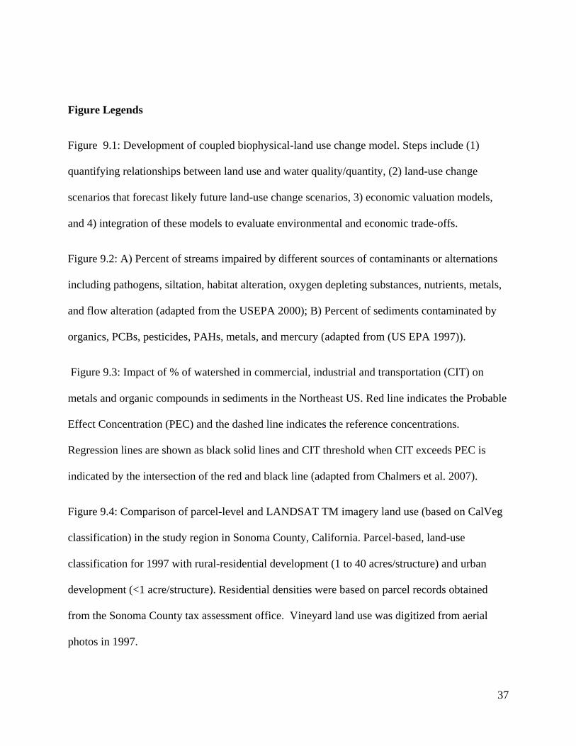
Figure 9.1: Development of coupled biophysical-land use change model. Steps include (1)
quantifying relationships between land use and water quality/quantity, (2) land-use change
scenarios that forecast likely future land-use change scenarios, 3) economic valuation models,
and 4) integration of these models to evaluate environmental and economic trade-offs.
Figure 9.2: A) Percent of streams impaired by different sources of contaminants or alternations
including pathogens, siltation, habitat alteration, oxygen depleting substances, nutrients, metals,
and flow alteration (adapted from the USEPA 2000); B) Percent of sediments contaminated by
organics, PCBs, pesticides, PAHs, metals, and mercury (adapted from (US EPA 1997)).
Figure 9.3: Impact of % of watershed in commercial, industrial and transportation (CIT) on
metals and organic compounds in sediments in the Northeast US. Red line indicates the Probable
Effect Concentration (PEC) and the dashed line indicates the reference concentrations.
Regression lines are shown as black solid lines and CIT threshold when CIT exceeds PEC is
indicated by the intersection of the red and black line (adapted from Chalmers et al. 2007).
Figure 9.4: Comparison of parcel-level and LANDSAT TM imagery land use (based on CalVeg
classification) in the study region in Sonoma County, California. Parcel-based, land-use
classification for 1997 with rural-residential development (1 to 40 acres/structure) and urban
development (<1 acre/structure). Residential densities were based on parcel records obtained
from the Sonoma County tax assessment office. Vineyard land use was digitized from aerial
photos in 1997.
38
Figure 9.5: Initial conditions of land-use development in the study watersheds and cost per parcel
area.
Figure 9.6: Change in probability distribution of spawning substrate quality with forecasted
land-use change and probability of loss of high-quality substrate/ land cost in least to most
developed watersheds in the Russian River Basin. The watersheds colored light grey represent
the lowest cost option for conserving high-quality spawning habitat.
39
Figure 9.1
40
Figure 9.2

41
Figure 9.3
42
Figure 9.4

43
Figure 9.5

44
Figure 9.6

45
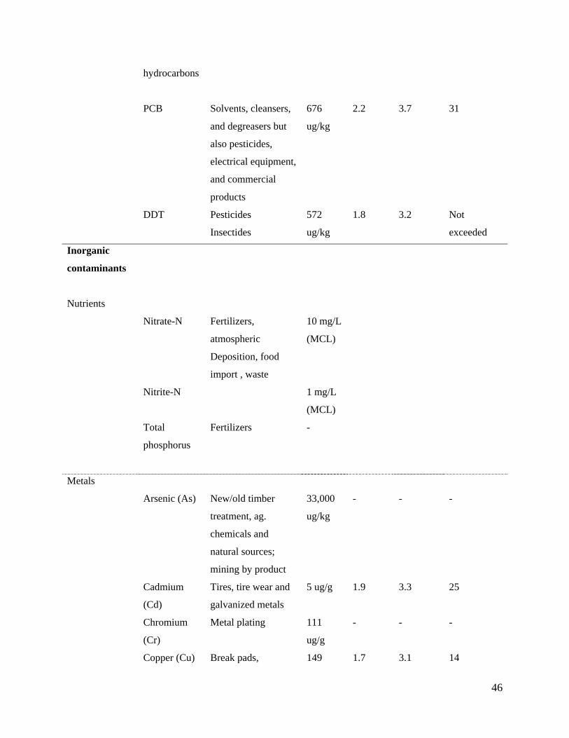
Table 1: Contaminants, sources of organic pollutants, nutrients, and metals, Probable Effect
Concentration (PEC) for sediments (in ug/g or ug/kg sediment) or Maximum contaminant level (MCL)
for drinking water (in mg/L), and predicted enrichment factor (EF) from conversion from rural (R) to
suburban (S) to urban land use (U). Percent commercial, industrial, and transportation (CIT) or
impervious surface area (ISC) is used as an index of urban intensity. Drinking water standards are
specified because regional water quality standards vary for rivers and streams (from Chalmers et al.
2007).
Contaminants Sources PEC
or
MCL
EF
(R to S)
EF
(S to U)
Threshold
CIT or ISC
> PEC or
EPA
Organic
Pollutants
Pathogenic
Escherichia
coli (E. coli)
Enteric
bacteria
Viruses
Septic, domestic
animals,
wildlife, or
agriculture
0 MCL
400
MPN/
100ml*
10-20%
ISC*
Toxic organic
Polyaromatic
hydrocarbons
(PAH)
By products of fossil
fuel combustion in
automobiles, power
plants, and heating
facilities.
Creosote and
roofing tar
Coal-tar and asphalt
sealant
22,800
ug/kg
6.1 5.2 13
Halogenated
46
hydrocarbons
PCB Solvents, cleansers,
and degreasers but
also pesticides,
electrical equipment,
and commercial
products
676
ug/kg
2.2 3.7 31
DDT Pesticides
Insectides
572
ug/kg
1.8 3.2 Not
exceeded
Inorganic
contaminants
Nutrients
Nitrate-N Fertilizers,
atmospheric
Deposition, food
import , waste
10 mg/L
(MCL)
Nitrite-N 1 mg/L
(MCL)
Total
phosphorus
Fertilizers -
Metals
Arsenic (As) New/old timber
treatment, ag.
chemicals and
natural sources;
mining by product
33,000
ug/kg
- - -
Cadmium
(Cd)
Tires, tire wear and
galvanized metals
5 ug/g
1.9 3.3 25
Chromium
(Cr)
Metal plating 111
ug/g
- - -
Copper (Cu) Break pads, 149 1.7 3.1 14

47
residential
algaecides, wood
preservatives,
landscaping
materials
ug/g
Mercury
(Hg)
Industrial waste,
mining, fuels
1.06
ug/g
1.7 3.1 23
Lead (Pb) Old housing (leaded
paint and fuel)
128
ug/g
1.9 3.4 3
Zinc (Zn) New urban surfaces,
rooftops, wood
preservative
459
ug/g
2 3.5 10
Sediments New construction,
roads, etc
*for water quality criterion in Georgia (Schoonover and Lockaby 2006).

48
Table 2: Steps to develop coupled environmental impact model and land use change model for guiding decision making, planning, ecosystem management, and conservation
Modeling components Steps
1. Environmental data for
environmental response
modeling
a. Collect spatial data on water
quality/quantity/habitat
b. Delineate scale of analysis in-line with scale
of land use data
c. Select statistical model to examine potential
causal relationships
d. Perform variable selection
e. Select best models
f. Test resulting models on an alternate data set
2. Land use change modeling a. Acquire land-use data at a parcel scale
b. Consolidate data into relevant land-use
categories
c. Derive land use variables
d. Calculate other relevant variables
3. Economic valuation modeling
a. Develop empirically based valuation model
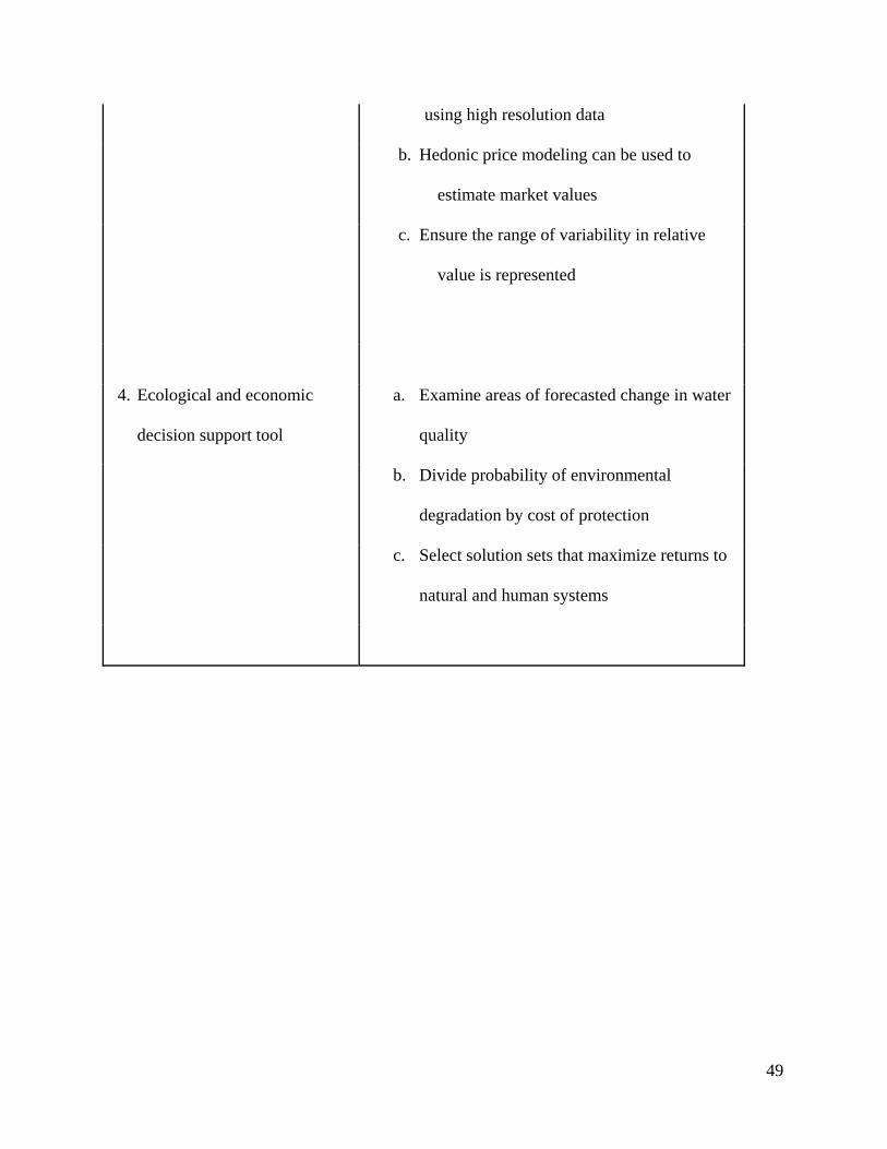
49
using high resolution data
b. Hedonic price modeling can be used to
estimate market values
c. Ensure the range of variability in relative
value is represented
4. Ecological and economic
decision support tool
a. Examine areas of forecasted change in water
quality
b. Divide probability of environmental
degradation by cost of protection
c. Select solution sets that maximize returns to
natural and human systems