Embed Size (px)
Citation preview
Copyright © 2011 Pearson Addison-Wesley. All rights reserved.
Chapter 9 Noncompetitive Markets and Inefficiency

Copyright © 2011 Pearson Addison-Wesley. All rights reserved. 9-2
FIGURE 9.BP.1 Market Structures and Their Characteristics

Copyright © 2011 Pearson Addison-Wesley. All rights reserved. 9-3
Monopoly • Monopoly Characteristics:
– 1 firm, no close substitutes, so the firm can set Price.
– Downward-sloping Demand Curve • The monopoly’s D curve is the mkt. D curve
– Barriers to Entry: factors keep out competitors
Copyright © 2011 Pearson Addison-Wesley. All rights reserved. 9-4
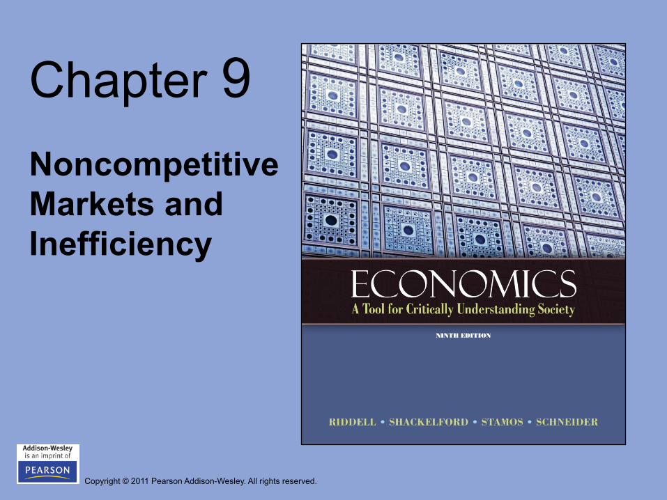
Barriers to Entry
• Economies of Scale (Natural Monopoly): – More efficient to be big – Declining LRAC curve, better to have only 1 firm
• Exclusive Ownership of a Unique Resource – Alcoa & Bauxite, Diamonds & DeBeers
• Govt. Granted Monopoly – Franchises granted to cable co., electric co., post office
• Patents & Copyrights – Monopoly on a drug formula (AZT), operating system (Windows),
etc. • The existence of Barriers to entry means that a monopolist
CAN earn economic profit in long run
Copyright © 2011 Pearson Addison-Wesley. All rights reserved. 9-5
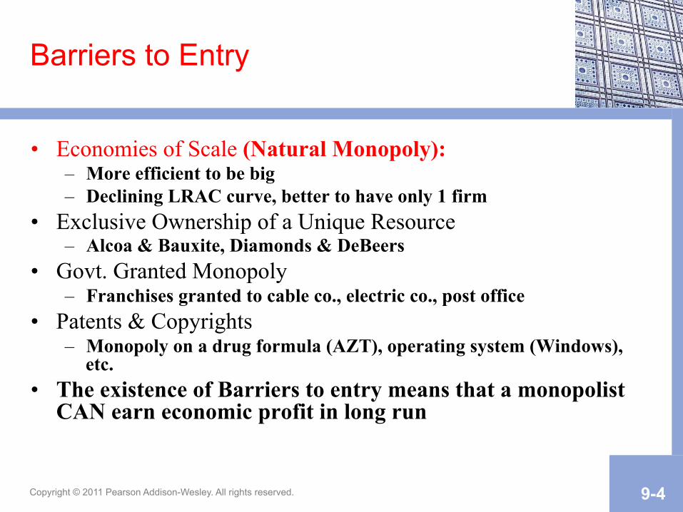
Profit Max. for a Monopolist: produce as long as MR�MC, but MR�P
Perfect Competition, MR=P Monopoly, P>MR
P Q TR MR P Q TR MR
10 1 10 10 10 1 10 10
10 2 20 10 9 2 18 8
10 3 30 10 8 3 24 6
10 4 40 10 7 4 28 4
10 5 50 10 6 5 30 2
10 6 60 10 5 6 30 0
Copyright © 2011 Pearson Addison-Wesley. All rights reserved. 9-6
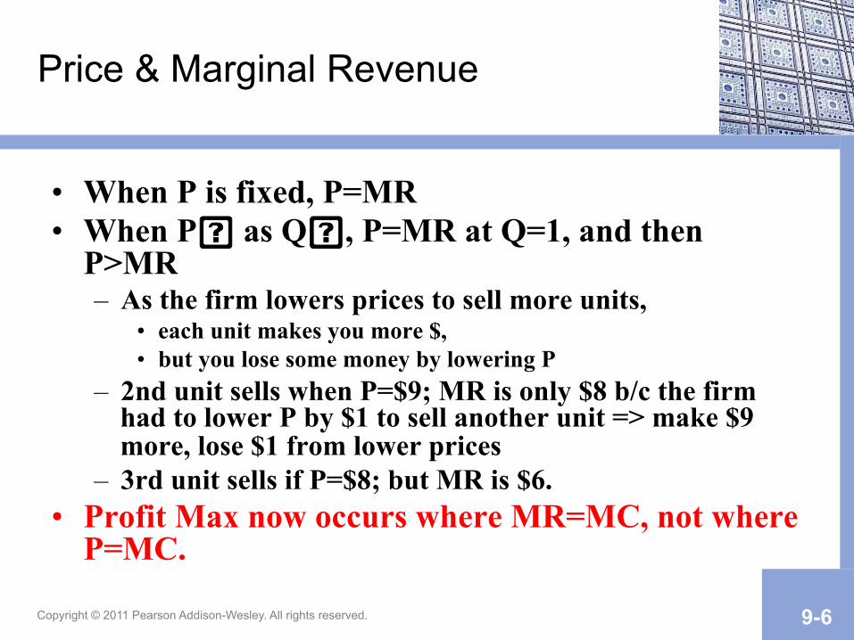
• When P is fixed, P=MR • When P� as Q�, P=MR at Q=1, and then
P>MR – As the firm lowers prices to sell more units,
• each unit makes you more $, • but you lose some money by lowering P
– 2nd unit sells when P=$9; MR is only $8 b/c the firm had to lower P by $1 to sell another unit => make $9 more, lose $1 from lower prices
– 3rd unit sells if P=$8; but MR is $6. • Profit Max now occurs where MR=MC, not where
P=MC.
Price & Marginal Revenue

Copyright © 2011 Pearson Addison-Wesley. All rights reserved. 9-7
D & MR under Perfect Competition vs. Monopoly
D=MR
D
MR
P P
Q Q
Perfect Competition Monopoly
Copyright © 2011 Pearson Addison-Wesley. All rights reserved. 9-8
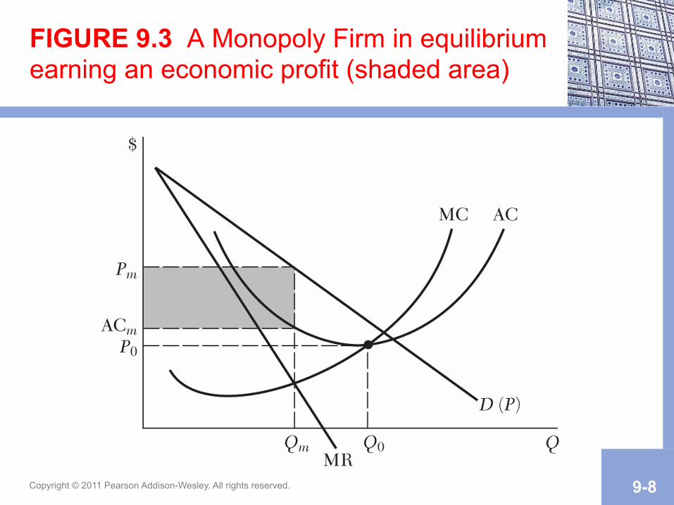
FIGURE 9.3 A Monopoly Firm in equilibrium earning an economic profit (shaded area)
Copyright © 2011 Pearson Addison-Wesley. All rights reserved. 9-9
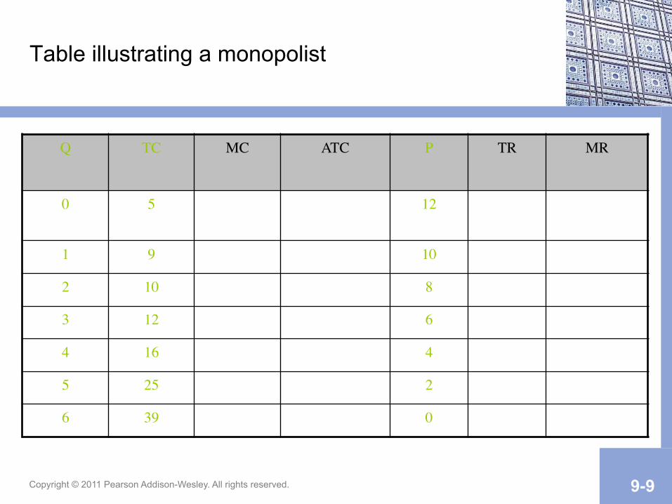
Table illustrating a monopolist
Q TC MC ATC P TR MR
0 5 12
1 9 10
2 10 8
3 12 6
4 16 4
5 25 2
6 39 0
Copyright © 2011 Pearson Addison-Wesley. All rights reserved. 9-10
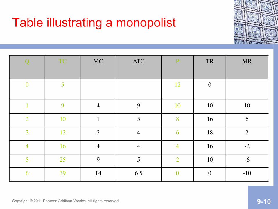
Table illustrating a monopolist
Q TC MC ATC P TR MR
0 5 12 0
1 9 4 9 10 10 10
2 10 1 5 8 16 6
3 12 2 4 6 18 2
4 16 4 4 4 16 -2
5 25 9 5 2 10 -6
6 39 14 6.5 0 0 -10
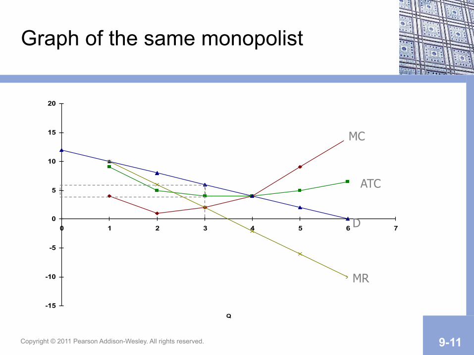
Copyright © 2011 Pearson Addison-Wesley. All rights reserved. 9-11
Graph of the same monopolist
-15
-10
-5
0
5
10
15
20
0 1 2 3 4 5 6 7
Q
ATC
D
MR
MC
Copyright © 2008 Pearson Addison-Wesley. All rights reserved. 9-12
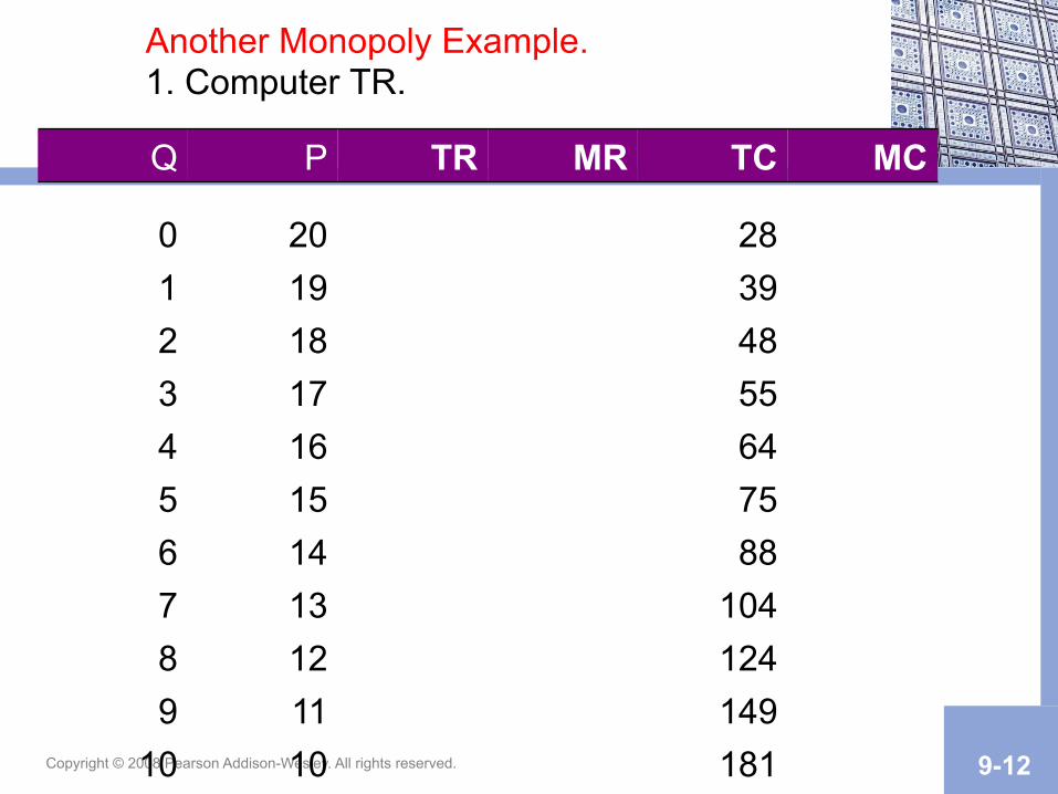
Another Monopoly Example. 1. Computer TR.
Q P TR MR TC MC
0 20 28 1 19 39 2 18 48 3 17 55 4 16 64 5 15 75 6 14 88 7 13 104 8 12 124 9 11 149
10 10 181
Copyright © 2008 Pearson Addison-Wesley. All rights reserved. 9-13
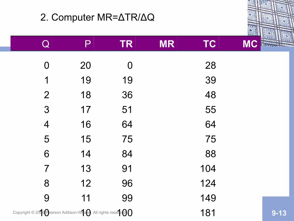
2. Computer MR=ΔTR/ΔQ
Q P TR MR TC MC
0 20 0 28 1 19 19 39 2 18 36 48 3 17 51 55 4 16 64 64 5 15 75 75 6 14 84 88 7 13 91 104 8 12 96 124 9 11 99 149
10 10 100 181
Copyright © 2008 Pearson Addison-Wesley. All rights reserved. 9-14
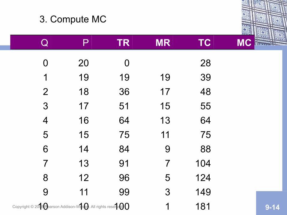
3. Compute MC
Q P TR MR TC MC
0 20 0 28 1 19 19 19 39 2 18 36 17 48 3 17 51 15 55 4 16 64 13 64 5 15 75 11 75 6 14 84 9 88 7 13 91 7 104 8 12 96 5 124 9 11 99 3 149
10 10 100 1 181

Copyright © 2008 Pearson Addison-Wesley. All rights reserved. 9-15
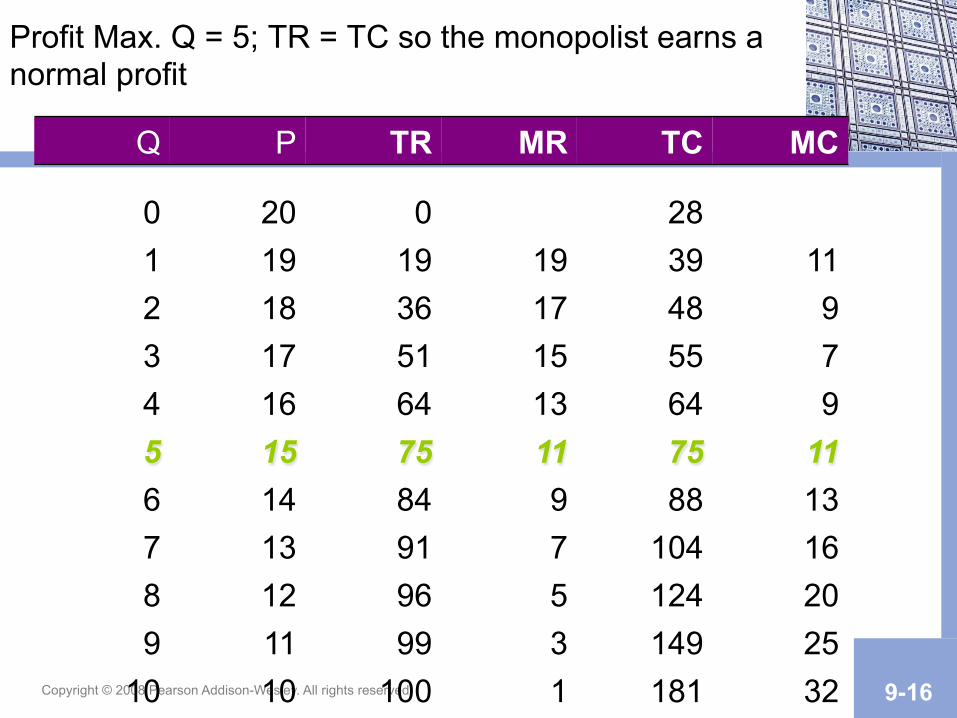
4. Determine the Profit Maximizing Level of Output and Compute Profit or Loss
Q P TR MR TC MC
0 20 0 28 1 19 19 19 39 11 2 18 36 17 48 9 3 17 51 15 55 7 4 16 64 13 64 9 5 15 75 11 75 11 6 14 84 9 88 13 7 13 91 7 104 16 8 12 96 5 124 20 9 11 99 3 149 25
10 10 100 1 181 32
Copyright © 2008 Pearson Addison-Wesley. All rights reserved. 9-16
Profit Max. Q = 5; TR = TC so the monopolist earns a normal profit
Q P TR MR TC MC
0 20 0 28 1 19 19 19 39 11 2 18 36 17 48 9 3 17 51 15 55 7 4 16 64 13 64 9 5 15 75 11 75 11 6 14 84 9 88 13 7 13 91 7 104 16 8 12 96 5 124 20 9 11 99 3 149 25
10 10 100 1 181 32
Copyright © 2011 Pearson Addison-Wesley. All rights reserved. 9-17
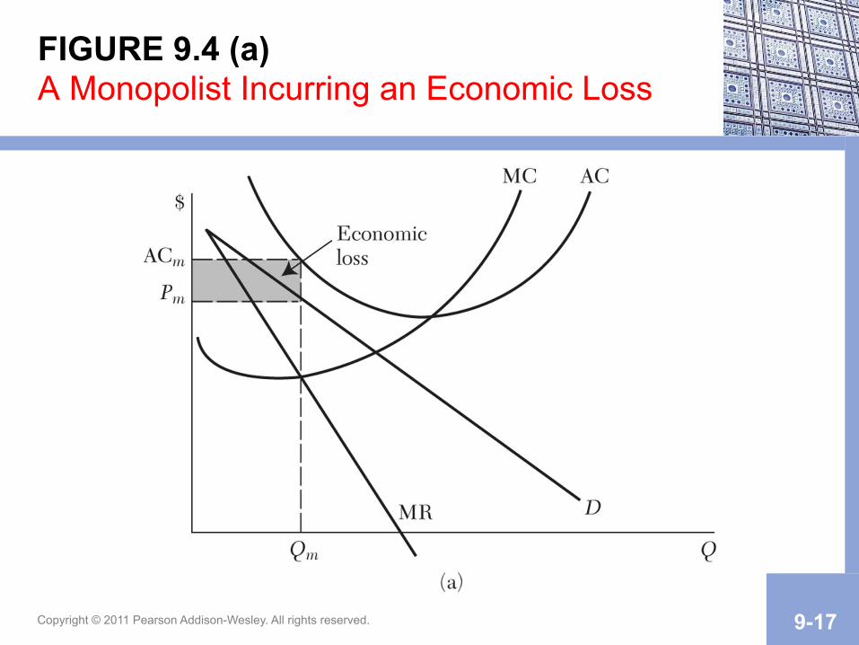
FIGURE 9.4 (a) A Monopolist Incurring an Economic Loss
Copyright © 2011 Pearson Addison-Wesley. All rights reserved. 9-18
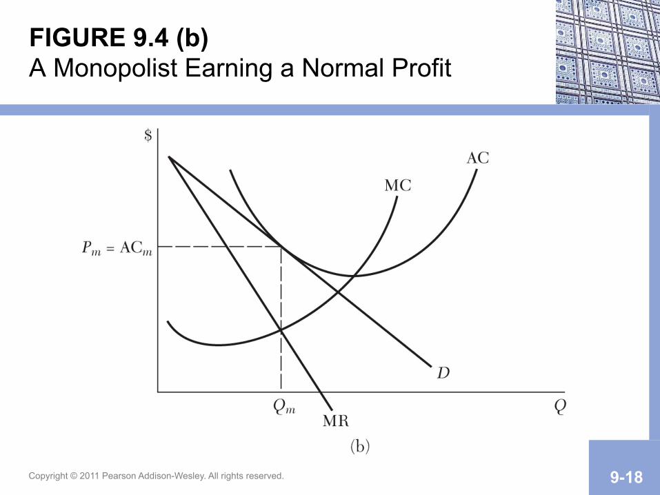
FIGURE 9.4 (b) A Monopolist Earning a Normal Profit

Copyright © 2011 Pearson Addison-Wesley. All rights reserved. 9-19
TABLE 9.1 Monopoly Revenue and Cost

Copyright © 2011 Pearson Addison-Wesley. All rights reserved. 9-20
FIGURE 9.1 Monopoly Demand and Marginal Revenue
Copyright © 2011 Pearson Addison-Wesley. All rights reserved. 9-21
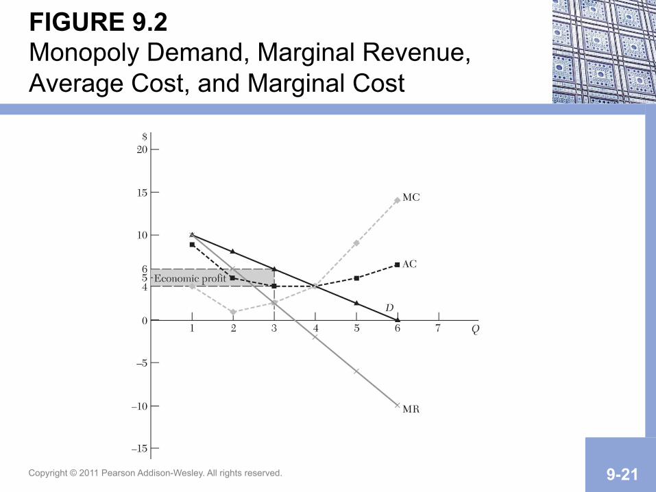
FIGURE 9.2 Monopoly Demand, Marginal Revenue, Average Cost, and Marginal Cost
Copyright © 2011 Pearson Addison-Wesley. All rights reserved. 9-22
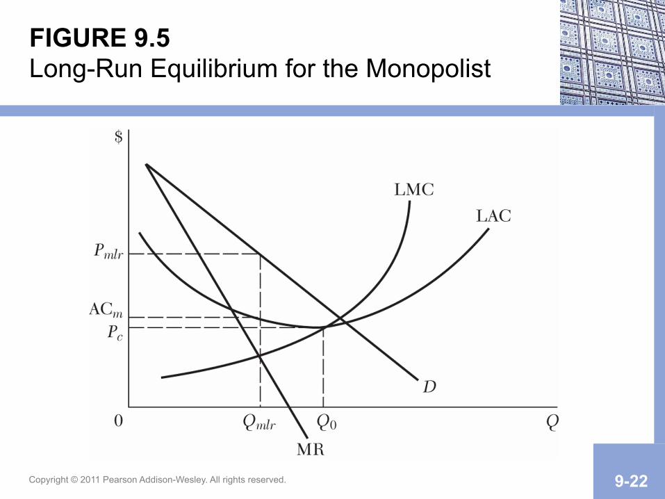
FIGURE 9.5 Long-Run Equilibrium for the Monopolist
Copyright © 2011 Pearson Addison-Wesley. All rights reserved. 9-23
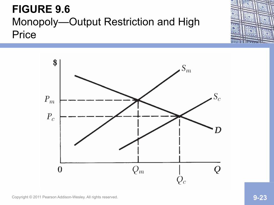
FIGURE 9.6 Monopoly—Output Restriction and High Price
Copyright © 2011 Pearson Addison-Wesley. All rights reserved. 9-24
Monopolistic Competition
Characteristics: • Easy Entry and Exit
– No significant barriers to entry – No long term economic profits
• Large number of firms – Firms can be small or large, but not dominant
• Products are close but not perfect substitutes (product differentiation) – Non-price competition (advertising)
Copyright © 2011 Pearson Addison-Wesley. All rights reserved. 9-25
Entry and Exit in Monopolistic Competition
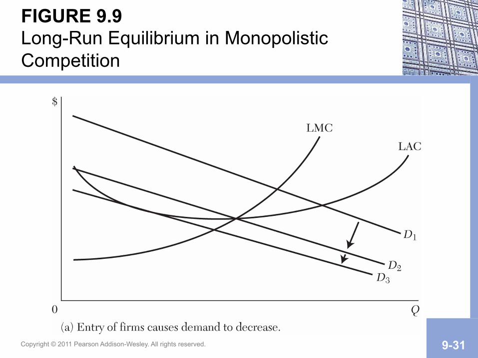
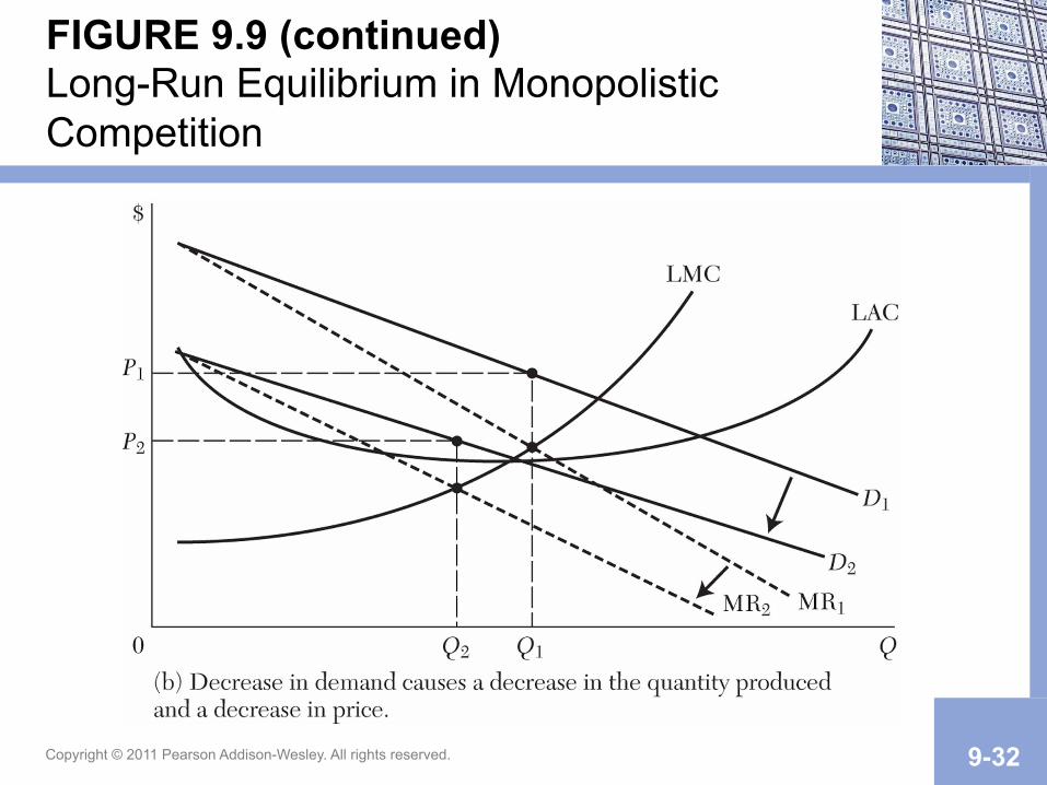
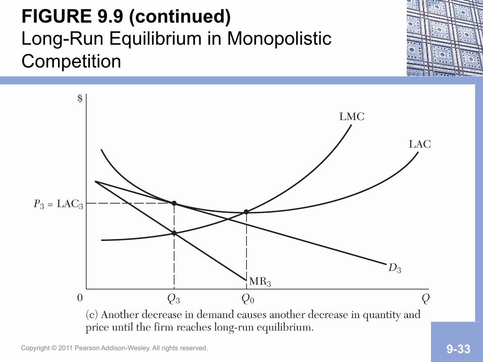
• Economic profits encourage more firms to enter – This creates more substitutes for existing brands – Decreasing the demand curve for existing firms – This process continues until firms earn a normal
profit
Copyright © 2011 Pearson Addison-Wesley. All rights reserved. 9-26
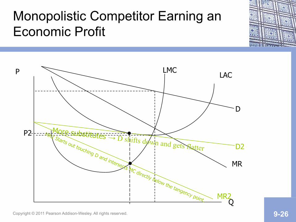
Monopolistic Competitor Earning an Economic Profit
D
LAC LMC
MR
P
Q
D2
More substitutes → D shifts down and gets flatter
●
MR2
●
MR2 Starts out touching D and intersects MC directly below the tangency point.
P2
Copyright © 2011 Pearson Addison-Wesley. All rights reserved. 9-27
• This means fewer substitutes for remaining products
• Increasing the demand curve for remaining firms
• This process continues until firms earn a normal profit
Economic losses cause firms to exit

Copyright © 2011 Pearson Addison-Wesley. All rights reserved. 9-28
Monopolistic Competitor with an Economic Loss
D
LAC LMC
MR
P
Q
D2
Fewer substitutes → D increases and gets steeper
●
MR2
MR2 starts out touching D and intersects MC directly below the tangency point
Copyright © 2011 Pearson Addison-Wesley. All rights reserved. 9-29
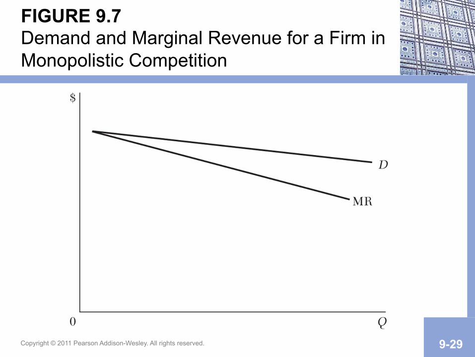
FIGURE 9.7 Demand and Marginal Revenue for a Firm in Monopolistic Competition
Copyright © 2011 Pearson Addison-Wesley. All rights reserved. 9-30
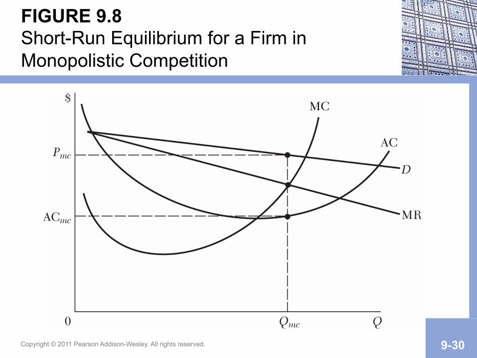
FIGURE 9.8 Short-Run Equilibrium for a Firm in Monopolistic Competition
Copyright © 2011 Pearson Addison-Wesley. All rights reserved. 9-31
FIGURE 9.9 Long-Run Equilibrium in Monopolistic Competition
Copyright © 2011 Pearson Addison-Wesley. All rights reserved. 9-32
FIGURE 9.9 (continued) Long-Run Equilibrium in Monopolistic Competition
Copyright © 2011 Pearson Addison-Wesley. All rights reserved. 9-33
FIGURE 9.9 (continued) Long-Run Equilibrium in Monopolistic Competition
Copyright © 2011 Pearson Addison-Wesley. All rights reserved. 9-34
OLIGOPOLY • Key Characteristics:
– Substantial Barriers to Entry – Dominated by a FEW LARGE FIRMS – INTERDEPENDENCE AMONG FIRMS
• Interdependence generates non-price competition (ads) and potentially
• INCENTIVES TO COLLUDE, merge
Copyright © 2011 Pearson Addison-Wesley. All rights reserved. 9-35
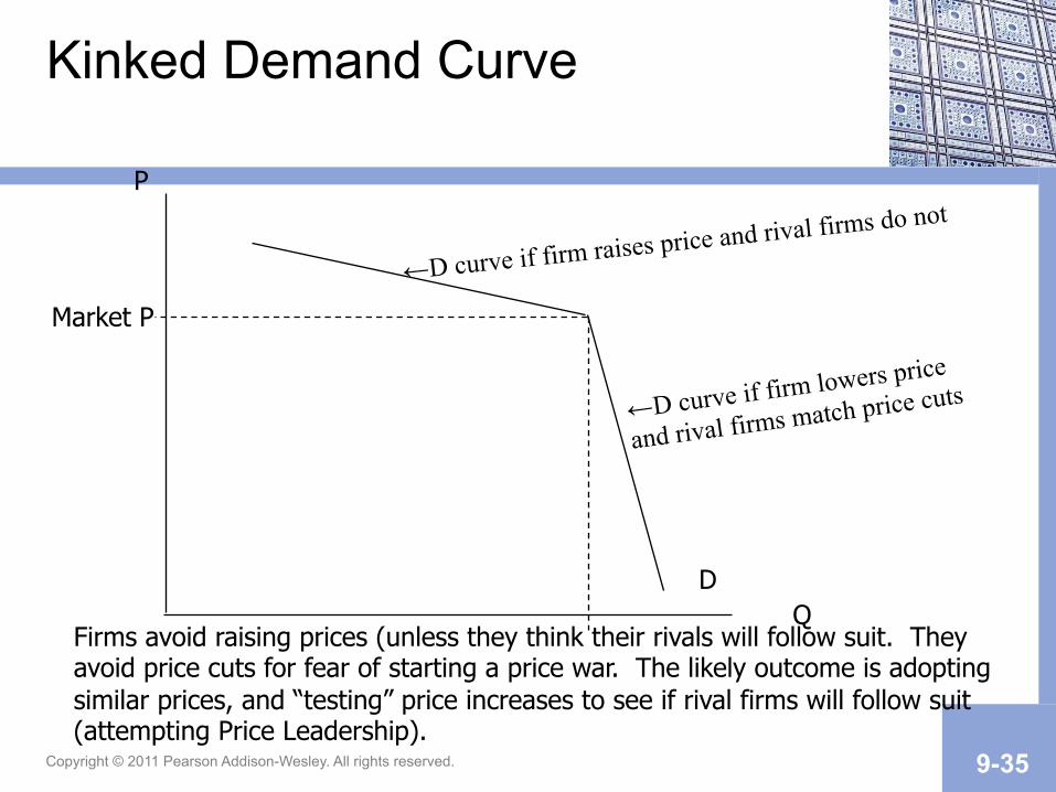
Kinked Demand Curve
P
Q D
←D curve if firm raises price and rival firms do not
←D curve if firm lowers price
and rival firms match price cuts
Market P
Firms avoid raising prices (unless they think their rivals will follow suit. They avoid price cuts for fear of starting a price war. The likely outcome is adopting similar prices, and “testing” price increases to see if rival firms will follow suit (attempting Price Leadership).

Copyright © 2011 Pearson Addison-Wesley. All rights reserved.
Game Theory illustrates the interdependence of firms, and the incentives they face

Copyright © 2011 Pearson Addison-Wesley. All rights reserved. 9-37
Payoff matrix showing profits of two firms when both have dominant strategies
Giant’s Advertising Expenditures
Low Expenditures High Expenditures
Weis’ Advertising Expenditures
Low Expenditures
Weis Profits: $300,000 Giant Profits: $300,000
Weis Profits: $100,000 Giant Profits: $400,000
High Expenditures
Weis Profits: $400,000 Giant Profits: $100,000
Weis Profits: $200,000 Giant Profits: $200,000
A dominant strategy exists if profits are higher no matter when the rival does.
Both Weis and Giant have a dominant strategy: High Ad Expenditures.
In this case, an equilibrium solution occurs in the lower right hand cell of the payoff matrix.
Copyright © 2011 Pearson Addison-Wesley. All rights reserved. 9-38
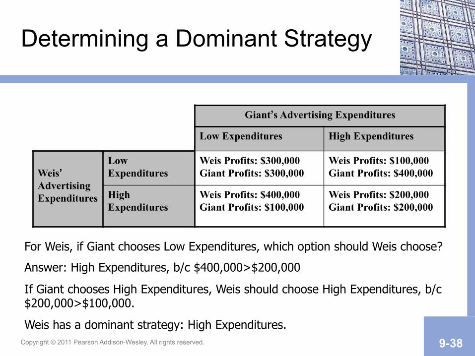
Determining a Dominant Strategy
Giant’s Advertising Expenditures
Low Expenditures High Expenditures
Weis’ Advertising Expenditures
Low Expenditures
Weis Profits: $300,000 Giant Profits: $300,000
Weis Profits: $100,000 Giant Profits: $400,000
High Expenditures
Weis Profits: $400,000 Giant Profits: $100,000
Weis Profits: $200,000 Giant Profits: $200,000
For Weis, if Giant chooses Low Expenditures, which option should Weis choose?
Answer: High Expenditures, b/c $400,000>$200,000
If Giant chooses High Expenditures, Weis should choose High Expenditures, b/c $200,000>$100,000.
Weis has a dominant strategy: High Expenditures.
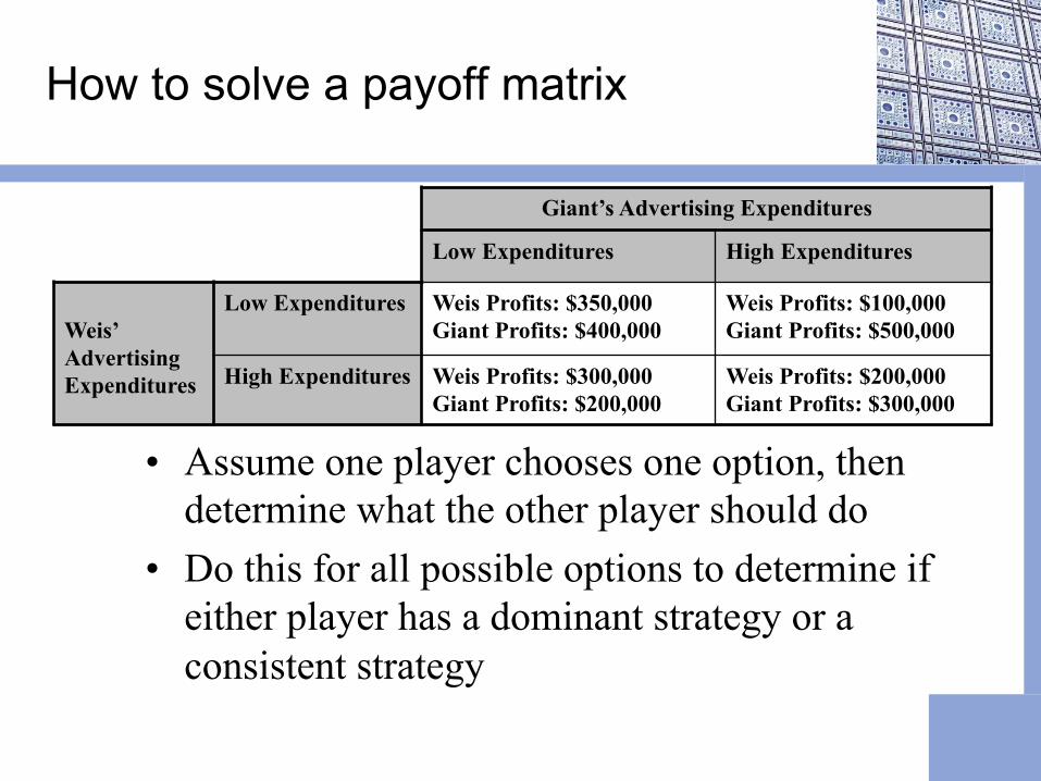
How to solve a payoff matrix
• Assume one player chooses one option, then determine what the other player should do
• Do this for all possible options to determine if either player has a dominant strategy or a consistent strategy
Giant’s Advertising Expenditures
Low Expenditures High Expenditures
Weis’ Advertising Expenditures
Low Expenditures Weis Profits: $350,000 Giant Profits: $400,000
Weis Profits: $100,000 Giant Profits: $500,000
High Expenditures Weis Profits: $300,000 Giant Profits: $200,000
Weis Profits: $200,000 Giant Profits: $300,000

• If Weis chooses Low, what should Giant do to make the most money?
Giant’s Advertising Expenditures
Low Expenditures High Expenditures
Weis’ Advertising Expenditures
Low Expenditures Giant Profits: $400,000 Giant Profits: $500,000
High Expenditures
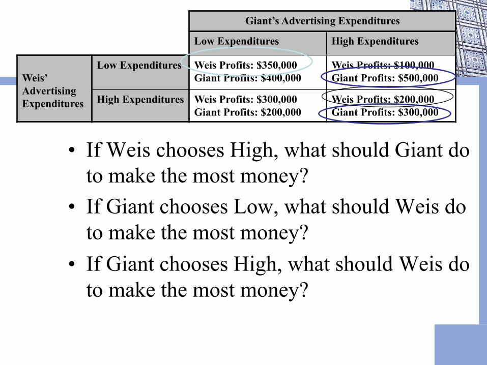
• If Weis chooses High, what should Giant do to make the most money?
• If Giant chooses Low, what should Weis do to make the most money?
• If Giant chooses High, what should Weis do to make the most money?
Giant’s Advertising Expenditures
Low Expenditures High Expenditures
Weis’ Advertising Expenditures
Low Expenditures Weis Profits: $350,000 Giant Profits: $400,000
Weis Profits: $100,000 Giant Profits: $500,000
High Expenditures Weis Profits: $300,000 Giant Profits: $200,000
Weis Profits: $200,000 Giant Profits: $300,000
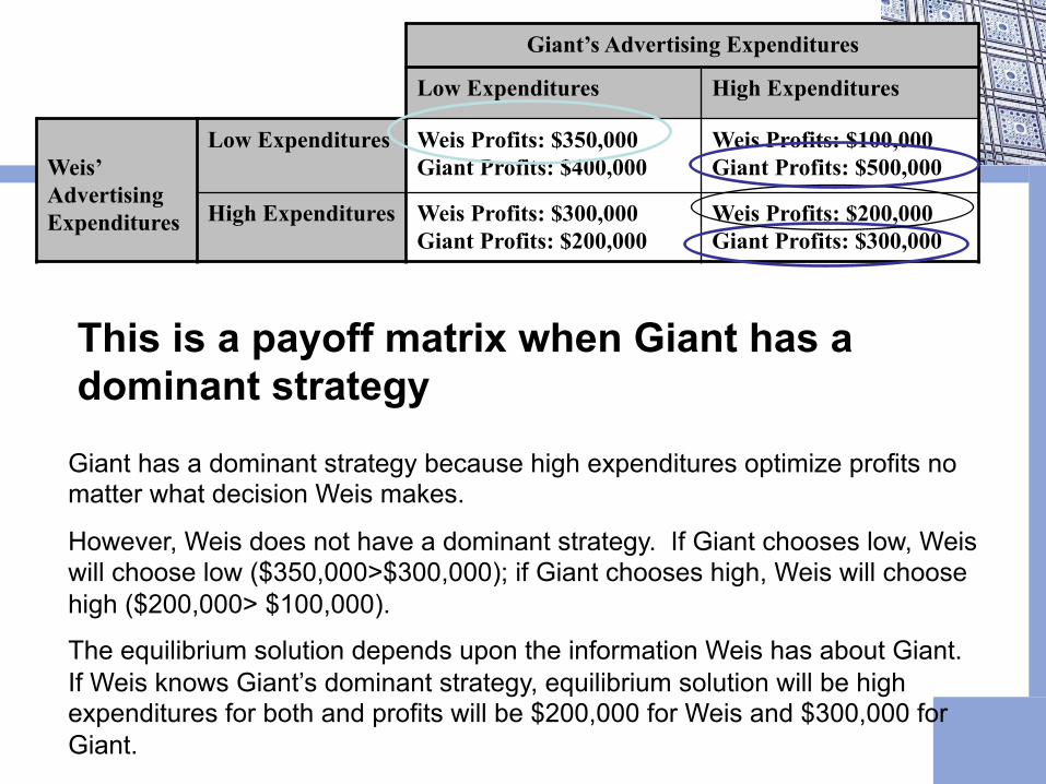
This is a payoff matrix when Giant has a dominant strategy
Giant has a dominant strategy because high expenditures optimize profits no matter what decision Weis makes.
However, Weis does not have a dominant strategy. If Giant chooses low, Weis will choose low ($350,000>$300,000); if Giant chooses high, Weis will choose high ($200,000> $100,000).
The equilibrium solution depends upon the information Weis has about Giant. If Weis knows Giant’s dominant strategy, equilibrium solution will be high expenditures for both and profits will be $200,000 for Weis and $300,000 for Giant.
Giant’s Advertising Expenditures
Low Expenditures High Expenditures
Weis’ Advertising Expenditures
Low Expenditures Weis Profits: $350,000 Giant Profits: $400,000
Weis Profits: $100,000 Giant Profits: $500,000
High Expenditures Weis Profits: $300,000 Giant Profits: $200,000
Weis Profits: $200,000 Giant Profits: $300,000
Copyright © 2011 Pearson Addison-Wesley. All rights reserved. 9-43
Collusion
• Cartel – Sellers join together to control output and/or prices. Illegal
in the US. – Example 1: OPEC – Example 2: Price fixing of Ivy League Schools – Example 3: Coke and Pepsi agreement on which product
would be on sale which week of the year • Price Leadership
– Market leader establishes the price, other firms follow suit. • Conscious parallelism
– Firms adopt identical prices without communication.
Copyright © 2011 Pearson Addison-Wesley. All rights reserved. 9-44
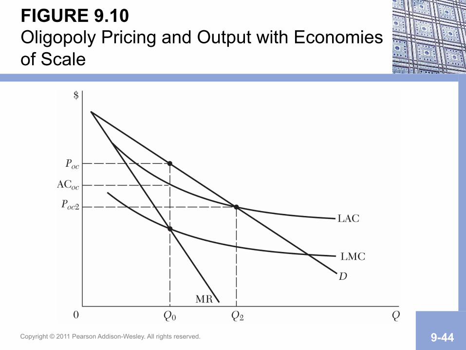
FIGURE 9.10 Oligopoly Pricing and Output with Economies of Scale
Copyright © 2011 Pearson Addison-Wesley. All rights reserved. 9-45
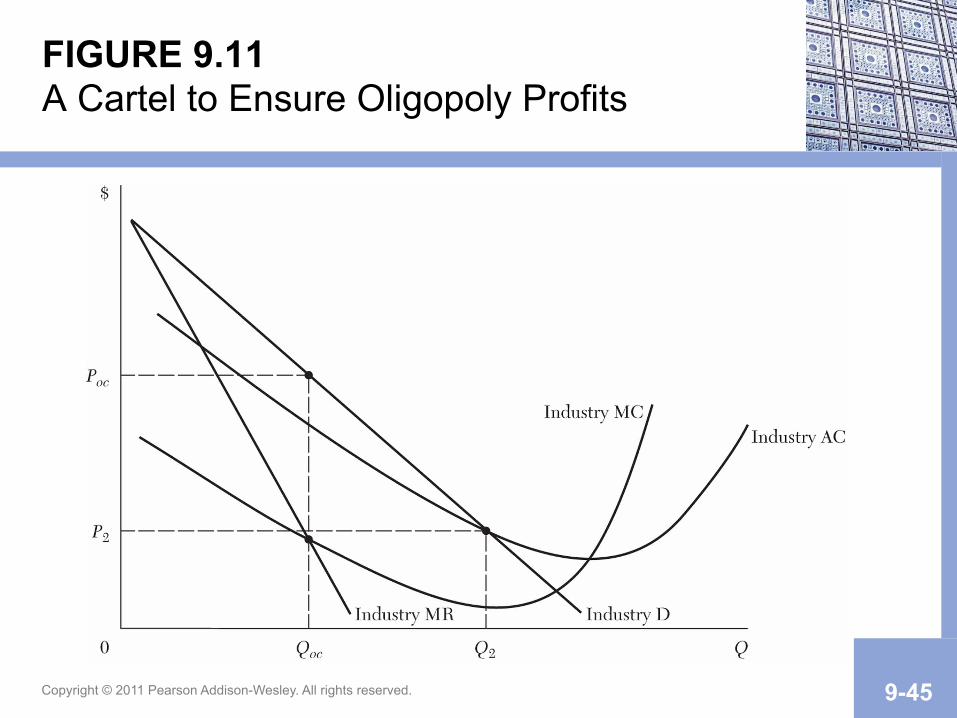
FIGURE 9.11 A Cartel to Ensure Oligopoly Profits
Copyright © 2011 Pearson Addison-Wesley. All rights reserved. 9-46
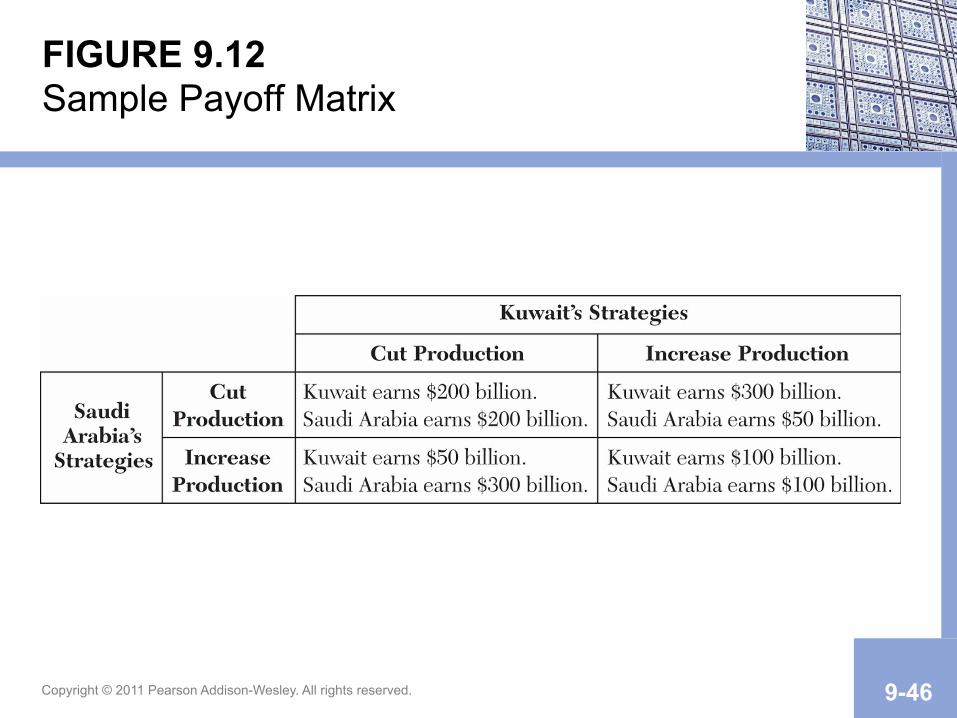
FIGURE 9.12 Sample Payoff Matrix
Copyright © 2011 Pearson Addison-Wesley. All rights reserved. 9-47
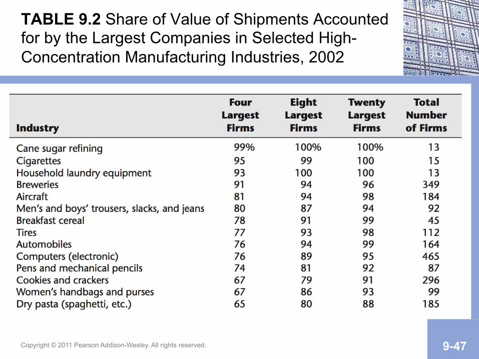
TABLE 9.2 Share of Value of Shipments Accounted for by the Largest Companies in Selected High-Concentration Manufacturing Industries, 2002
Copyright © 2011 Pearson Addison-Wesley. All rights reserved. 9-48
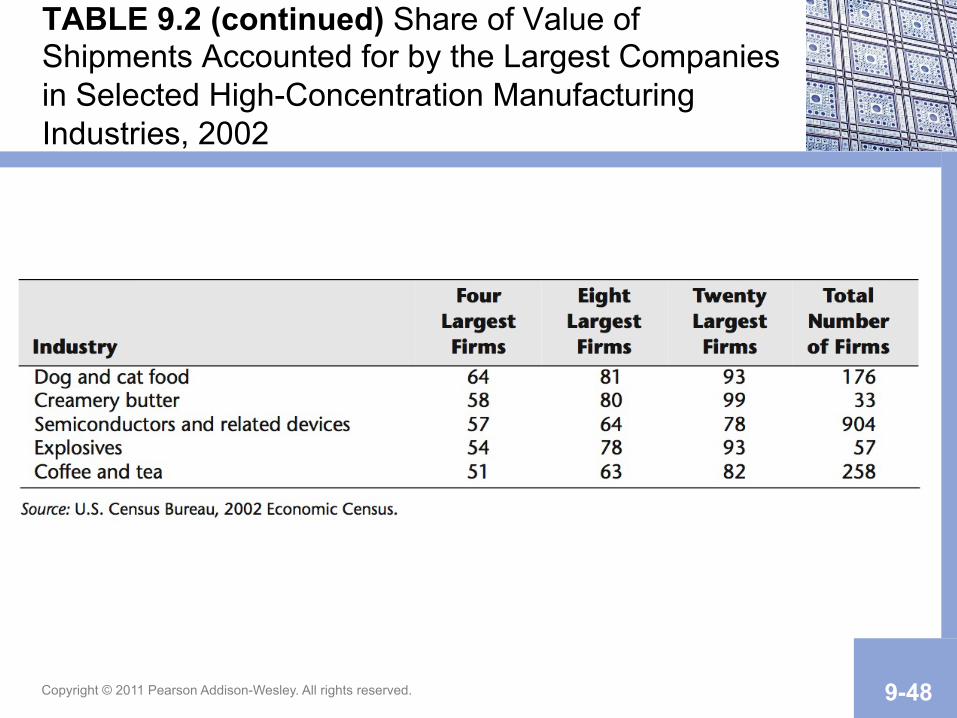
TABLE 9.2 (continued) Share of Value of Shipments Accounted for by the Largest Companies in Selected High-Concentration Manufacturing Industries, 2002
Copyright © 2011 Pearson Addison-Wesley. All rights reserved. 9-49
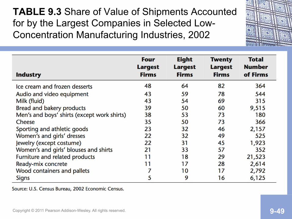
TABLE 9.3 Share of Value of Shipments Accounted for by the Largest Companies in Selected Low-Concentration Manufacturing Industries, 2002
Copyright © 2011 Pearson Addison-Wesley. All rights reserved. 9-50
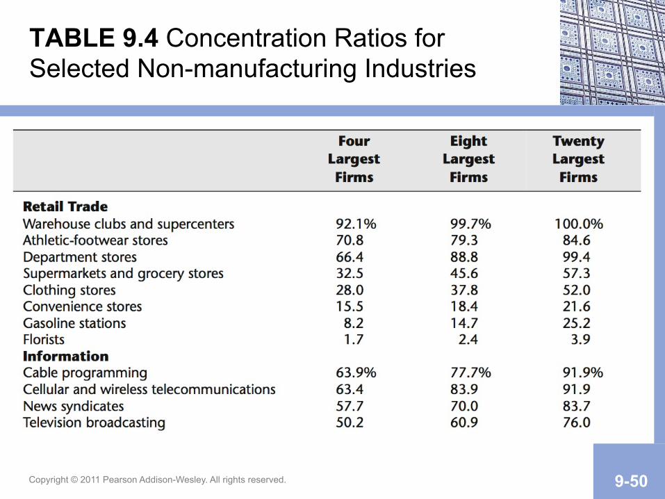
TABLE 9.4 Concentration Ratios for Selected Non-manufacturing Industries
Copyright © 2011 Pearson Addison-Wesley. All rights reserved. 9-51
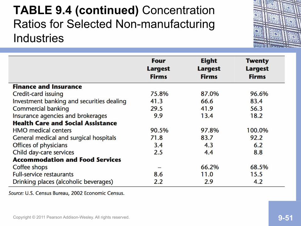
TABLE 9.4 (continued) Concentration Ratios for Selected Non-manufacturing Industries
Copyright © 2011 Pearson Addison-Wesley. All rights reserved. 9-52


![HRM Weis Orginal(MBA[1].Teheran).ppt](https://img.pdfslide.us/doc/110x75/54528b35b1af9f477e8b456f/hrm-weis-orginalmba1teheranppt.jpg)