Chapter 9 Differential Equations - Undergrad · PDF fileChapter 9 Differential Equations 9.1 Introduction A differential equation is a relationship between some (unknown) function

Chapter 9

Differential Equations

9.1 IntroductionA differential equation is a relationship between some (unknown) function and one of itsderivatives. Examples of differential equations were encountered in an earlier calculuscourse in the context of population growth, temperature of a cooling object, and speed of amoving object subjected to friction. In Section 4.2.4, we reviewed an example of a differ-ential equation for velocity, (4.8), and discussed its solution, but here, we present a moresystematic approach to solving such equations using a technique called separation of vari-ables. In this chapter, we apply the tools of integration to finding solutions to differentialequations. The importance and wide applicability of this topic cannot be overstated.

In this course, since we are concerned only with functions that depend on a singlevariable, we discuss ordinary differential equations (ODE’s), whereas later, after a mul-tivariate calculus course where partial derivatives are introduced, a wider class, of partialdifferential equations (PDE’s) can be studied. Such equations are encountered in many ar-eas of science, and in any quantitative analysis of systems where rates of change are linkedto the state of the system. Most laws of physics are of this form; for example, applyingthe familiar Newton’s law, F = ma, links the position of a pendulum’s mass to its accel-eration (second derivative of position).42 Many biological processes are also described bydifferential equations. The rate of growth of a population dN/dt depends on the size ofthat population at the given time N(t).

Constructing the differential equation that adequately represents a system of interestis an art that takes some thought and experience. In this process, which we call “modeling”,many simplifications are made so that the essential properties of a given system are cap-tured, leaving out many complicating details. For example, friction might be neglected in“modeling” a perfect pendulum. The details of age distribution might be neglected in mod-eling a growing population. Now that we have techniques for integration, we can devise anew approach to computing solutions of differential equations.

Given a differential equation and a starting value, the goal is to make a prediction

42Newton’s law states that force is proportional to acceleration. For a pendulum, the force is due to gravity, andthe acceleration is a second derivative of the x or y coordinate of the bob on the pendulum.

177

178 Chapter 9. Differential Equations

about the future behaviour of the system. This is equivalent to identifying the function thatsatisfies the given differential equation and initial value(s). We refer to such a function asthe solution to the initial value problem (IVP). In differential calculus, our explorationof differential equations was limited to those whose solution could be guessed, or whosesolution was supplied in advance. We also explored some of the fascinating geometric andqualitative properties of such equations and their predictions.

Now that we have techniques of integration, we can find the analytic solution to avariety of simple first-order differential equations (i.e. those involving the first derivativeof the unknown function). We will describe the technique of separation of variables. Thistechnique works for examples that are simple enough that we can isolate the dependentvariable (e.g. y) on one side of the equation, and the independent variable (e.g. time t) onthe other side.

9.2 Unlimited population growthWe start with a simple example that was treated thoroughly in the differential calculussemester of this course. We consider a population with per capita birth and mortality ratesthat are constant, irrespective of age, disease, environmental changes, or other effects. Weask how a population in such ideal circumstances would change over time. We build upa simple model (i.e. a differential equation) to describe this ideal case, and then proceedto find its solution. Solving the differential equation is accomplished by a new techniqueintroduced here, namely separation of variables. This reduces the problem to integrationand algebraic manipulation, allowing us to compute the population size at any time t. Bygoing through this process, we essentially convert information about the rate of change andstarting level of the population to a detailed prediction of the population at later times.43

9.2.1 A simple model for population growthLet y(t) represent the size of a population at time t. We will assume that at time t = 0, thepopulation level is specified, i.e. y(0) = y0 is some given constant. We want to find thepopulation at later times, given information about birth and mortality rates, (both of whichare here assumed to be constant over time).

The population changes through births and mortality. Suppose that b > 0 is the percapita average birth rate, and m > 0 the per capita average mortality rate. The assumptionthat b, m are both constants is a simplification that neglects many biological effects, butwill be used for simplicity in this first example.

The statement that the population increases through births and decreases due to mor-tality, can be restated as

rate of change of y = rate of births ! rate of mortality

where the rate of births is given by the product of the per capita average birth rate b and thepopulation size y. Similarly, the rate of mortality is given by my. Translating the rate of

43Of course, we must keep in mind that such predictions are based on simplifying assumptions, and are to betaken as an approximation of any real population growth.

9.2. Unlimited population growth 179

change into the corresponding derivative of y leads to

dy

dt= by ! my = (b ! m)y.

Let us define the new constant,k = b ! m.

Then k is the net per capita growth rate of the population. We can distinguish two possiblecases: b > m means that there are more births then deaths, so we expect the populationto grow. b < m means that there are more deaths than births, so that the population willeventually go extinct. There is also a marginal case that b = m, for which k = 0, where thepopulation does not change at all. To summarize, this simple model of unlimited growthleads to the differential equation and initial condition:

dy

dt= ky, y(0) = y0. (9.1)

Recall that a differential equation together with an initial condition is called an initial valueproblem. To find a solution to such a problem, we look for the function y(t) that describesthe population size at any future time t, given its initial size at time t = 0.

9.2.2 Separation of variables and integrationWe here introduce the technique, separation of variables, that will be used in all theexamples described in this chapter. Since the differential equation (9.1) is relatively simple,this first example will be relatively straightforward. We would like to determine y(t) giventhe differential equation

dy

dt= ky.

Rather than integrating this equation as is44, we use an alternate approach, consid-ering dt and dy as “differentials” in the sense defined in Section 6.1. We rearrange andrewrite the above equation in the form

1

ydy = k dt, (9.2)

This step of putting expressions involving the independent variable t on one side and ex-pressions involving the dependent variable y on the opposite side gives rise to the name“separation of variables”.

Now, the LHS of Eqn. (9.2) depends only on the variable y, and the RHS only on t.The constant k will not interfere with any integration step. Moreover, integrating each sideof Eqn. (9.2) can be carried out independently.

To determine the appropriate intervals for integration, we observe that when timesweeps over some interval 0 " t " T (from initial to final time), the value of y(t) will

44We may be tempted to integrate both sides of this equation with respect to the independent variable t, e.g.writing

!dydt

dt =!

ky dt + C, (where C is some constant), but this is not very useful, since the integral onthe right hand side (RHS) can only be carried out if we know the function y = y(t), which we are trying todetermine.


change over a corresponding interval y0 " y " y(T ). Here y0 is the given starting valueof y (prescribed by the initial condition in (9.1)). We do not yet know y(T ), but our goalis to find that value, i.e to predict the future behaviour of y. Integrating leads to

" y(T )

y0

1

ydy =

" T

0k dt = k

" T

0dt,

ln |y|####

y(T )

y0

= kt

####

T

0

,

ln |y(T )|! ln |y(0)| = k(T ! 0),

ln

####

y(T )

y0

####= kT,

y(T )

y0= ekT ,

y(T ) = y0ekT .

But this result holds for any arbitrary final time, T . In other words, since this is true for anytime we chose, we can set T = t, arriving at the desired solution

y(t) = y0ekt. (9.3)

The above formula relates the predicted value of y at any time t to its initial value, and toall the parameters of the problem. Observe that plugging in t = 0, we get y(0) = y0ekt =y0e0 = y0, so that the solution (9.3) satisfies the initial condition. We leave as an exercisefor the reader45 to validate that the function in(9.3) also satisfies the differential equation in(9.1).

By solving the initial value problem (9.1), we have determined that, under ideal con-ditions, when the net per capita growth rate t is constant, a population will grow expo-nentially with time. Recall that this validates results that we had encountered in our firstcalculus course.

9.3 Terminal velocity and steady statesHere we revisit the equation for velocity of a falling object that we first encountered in Sec-tion 4.2.4. We wish to derive the appropriate differential equation governing that velocity,and find the solution v(t) as a function of time. We will first reconsider the simplest case ofuniformly accelerated motion (i.e. where friction is neglected), as in Section 4.2.3. We theninclude friction, as in Section 4.2.4 and use the new technique of separation of variables toshortcut the method of solution.

45This kind of check is good practice and helps to spot errors. Simply differentiate Eqn. (9.3) and show that theresult is the same as k times the original function, as required by the equation (9.1).

9.3. Terminal velocity and steady states 181

9.3.1 Ignoring friction: the uniformly accelerated caseLet v(t) and a(t) be the velocity and the acceleration, respectively of an object fallingunder the force of gravity at time t. We take the positive direction to be downwards, forconvenience. Suppose that at time t = 0, the object starts from rest, i.e. the initial velocityof the object is known to be v(0) = 0. When friction is neglected, the object will accelerate,

a(t) = g,

which is equivalent to the statement that the velocity increases at a constant rate,

dv

dt= g. (9.4)

Because g is constant, we do not need to use separation of variables, i.e. we can integrateeach side of this equation directly46. Writing

"dv

dtdt =

"

g dt + C = g

"

dt + C,

where C is an integration constant, we arrive at

v(t) = gt + C. (9.5)

Here we have used (on the LHS) that v is the antiderivative of dv/dt. (equivalently, we cansimplify the integral

!dvdt dt =

!

dv = v). Plugging in v(0) = 0 into Eqn. (9.5) leads to0 = g · 0 + C = C, so the constant we need is C = 0 and the velocity satisfies

v(t) = gt.

We have just arrived at a result that parallels Eqn. (4.4) of Section 4.2.3 (in slightly differentnotation).

9.3.2 Including friction: the case of terminal velocityWhen a falling object experiences the force of friction, it cannot accelerate indefinitely. Infact, a frictional force retards the downwards motion. To a good approximation, that forceis proportional to the velocity.

A force balance for the falling object leads to

ma(t) = mg ! !v(t),

where ! is the frictional coefficient. For an object of constant mass, we can divide throughby m, so

a(t) = g !!

mv(t).

46It is important to note the distinction between this simple example and other cases where separation of vari-ables is required. It would not be wrong to use separation of variables to find the solution for Eqn. (9.4), but itwould just be “overkill”, since simple integration of the each side of the equation “as is” does the job.


Let k = !/m. Then, the velocity at any time satisfies the differential equation and initialcondition

dv

dt= g ! kv, v(0) = 0. (9.6)

We can find the solution to this differential equation and predict the velocity at any time tusing separation of variables.

terminal velocity

time t

velocity v

0.0 10.00.0

20.0

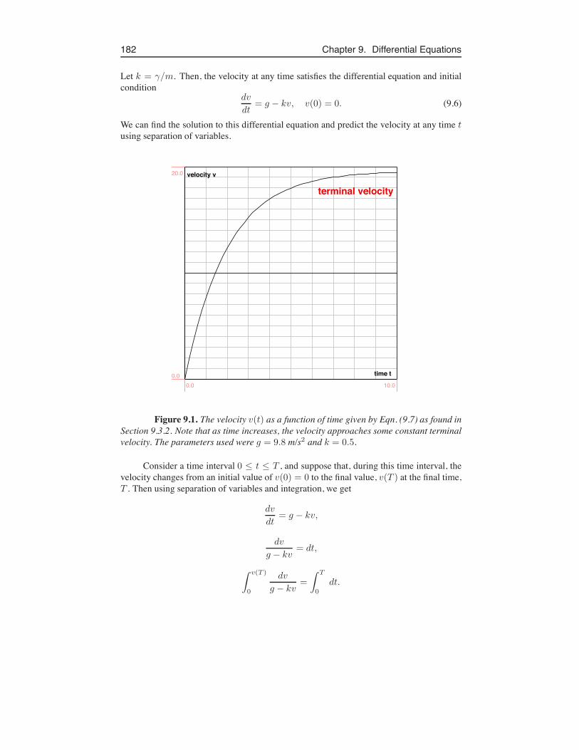
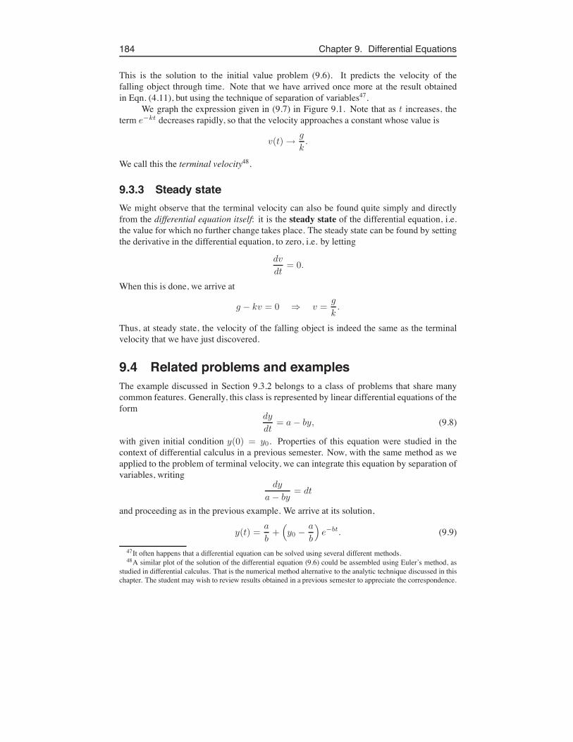
Figure 9.1. The velocity v(t) as a function of time given by Eqn. (9.7) as found inSection 9.3.2. Note that as time increases, the velocity approaches some constant terminalvelocity. The parameters used were g = 9.8 m/s2 and k = 0.5.

Consider a time interval 0 " t " T , and suppose that, during this time interval, thevelocity changes from an initial value of v(0) = 0 to the final value, v(T ) at the final time,T . Then using separation of variables and integration, we get

dv

dt= g ! kv,

dv

g ! kv= dt,

" v(T )

0

dv

g ! kv=

" T

0dt.

9.3. Terminal velocity and steady states 183

Substitute u = g ! kv for the integral on the left hand side. Then du = !kdv, dv =(!1/k)du, so we get an integral of the form

!1

k

"1

udu = !

1

kln |u|.

After replacing u by g ! kv, we arrive at

!1

kln |g ! kv|

####

v(T )

0

= t

####

T

0

.

We use the fact that v(0) = 0 to write this as

!1

k(ln |g ! kv(T )|! ln |g|) = T,

!1

k

$

ln

####

g ! kv(T )

g

####

%

= T,

ln

####

g ! kv(T )

g

####= !kT.

We are finished with the integration step, but the function we are trying to find, v(T )is still tangled up inside an expression involving the natural logarithm. Extricating it willinvolve some subtle reasoning about signs because there is an absolute value to contendwith. As a first step, we exponentiate both sides to remove the logarithm.

####

g ! kv(T )

g

####= e!kT # |g ! kv(T )| = ge!kT .

Because the constant g is positive, we could remove absolute values signs from it. Tosimplify further, we have to consider the sign of the term inside the absolute value in thenumerator. In the case we are considering here, v(0) = 0. This will mean that the quantityg ! kv(T ) is always be non-negative (i.e. g ! kv(T ) $ 0). We will verify this fact shortly.For the moment, supposing this is true, we can write

|g ! kv(T )| = g ! kv(T ) = ge!kT ,

and finally solve for v(T ) to obtain our final result,

v(T ) =g

k(1 ! e!kT ).

Here we note that v(T ) can never be larger than g/k since the term (1 ! e!kT ) is always" 1. Hence, we were correct in assuming that g ! kv(T ) $ 0.

As before, the above formula relating velocity to time holds for any choice of thefinal time T , so we can write, in general,

v(t) =g

k(1 ! e!kt). (9.7)


This is the solution to the initial value problem (9.6). It predicts the velocity of thefalling object through time. Note that we have arrived once more at the result obtainedin Eqn. (4.11), but using the technique of separation of variables47.

We graph the expression given in (9.7) in Figure 9.1. Note that as t increases, theterm e!kt decreases rapidly, so that the velocity approaches a constant whose value is

v(t) %g

k.

We call this the terminal velocity48.

9.3.3 Steady stateWe might observe that the terminal velocity can also be found quite simply and directlyfrom the differential equation itself: it is the steady state of the differential equation, i.e.the value for which no further change takes place. The steady state can be found by settingthe derivative in the differential equation, to zero, i.e. by letting

dv

dt= 0.

When this is done, we arrive at

g ! kv = 0 # v =g

k.

Thus, at steady state, the velocity of the falling object is indeed the same as the terminalvelocity that we have just discovered.

9.4 Related problems and examplesThe example discussed in Section 9.3.2 belongs to a class of problems that share manycommon features. Generally, this class is represented by linear differential equations of theform

dy

dt= a ! by, (9.8)

with given initial condition y(0) = y0. Properties of this equation were studied in thecontext of differential calculus in a previous semester. Now, with the same method as weapplied to the problem of terminal velocity, we can integrate this equation by separation ofvariables, writing

dy

a ! by= dt

and proceeding as in the previous example. We arrive at its solution,

y(t) =a

b+

&

y0 !a

b

'

e!bt. (9.9)

47It often happens that a differential equation can be solved using several different methods.48A similar plot of the solution of the differential equation (9.6) could be assembled using Euler’s method, as

studied in differential calculus. That is the numerical method alternative to the analytic technique discussed in thischapter. The student may wish to review results obtained in a previous semester to appreciate the correspondence.

9.4. Related problems and examples 185

The steps are left as an exercise for the reader.We observe that the steady state of the above equation is obtained by setting

dy

dt= a ! by = 0, i.e. y =

a

b.

Indeed the solution given in the formula (9.9) has the property that as t increases, theexponential term e!bt % 0 so that the term in large brackets will vanish and y % a/b.This means that from any initial value, y will approach its steady state level.

This equation has a number of important applications that arise in a variety of context.A few of these are mentioned below.

9.4.1 Blood alcoholLet y(t) be the level of alcohol in the blood of an individual during a party. Suppose thatthe average rate of drinking is gradual and constant (i.e. small sips are continually taken,so that the rate of input of alcohol is approximately constant). Further, assume that alcoholis detoxified in the liver at a rate proportional to its blood level. Then an equation of theform (9.8) would describe the blood level over the period of drinking. y(0) = 0 wouldsignify the absence of alcohol in the body at the beginning of the evening. The constant awould reflect the rate of intake per unit volume of the individual’s blood: larger people takelonger to “get drunk” for a given amount consumed49. The constant b represents the rate ofdecay of alcohol per unit time due to degradation by the liver, assumed constant50; younghealthy drinkers have a higher value of b than those who can no longer metabolize alcoholas efficiently.

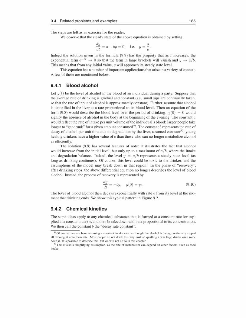
The solution (9.9) has several features of note: it illustrates the fact that alcoholwould increase from the initial level, but only up to a maximum of a/b, where the intakeand degradation balance. Indeed, the level y = a/b represents a steady state level (aslong as drinking continues). Of course, this level could be toxic to the drinker, and theassumptions of the model may break down in that region! In the phase of “recovery”,after drinking stops, the above differential equation no longer describes the level of bloodalcohol. Instead, the process of recovery is represented by

dy

dt= !by, y(0) = y0. (9.10)

The level of blood alcohol then decays exponentially with rate b from its level at the mo-ment that drinking ends. We show this typical pattern in Figure 9.2.

9.4.2 Chemical kineticsThe same ideas apply to any chemical substance that is formed at a constant rate (or sup-plied at a constant rate) a, and then breaks down with rate proportional to its concentration.We then call the constant b the “decay rate constant”.

49Of course, we are here assuming a constant intake rate, as though the alcohol is being continually sippedall evening at a uniform rate. Most people do not drink this way, instead quaffing a few large drinks over somehour(s). It is possible to describe this, but we will not do so in this chapter.

50This is also a simplifying assumption, as the rate of metabolism can depend on other factors, such as foodintake.


0

0.2

0.4

0.6

0.8

1

0 2 4 6 8 10

Blood Alcohol level

Figure 9.2. The level of alcohol in the blood is described by Eqn. (9.8) for the firsttwo hours of drinking. At t = 2h, the drinking stopped (so a = 0 from then on). The levelof alcohol in the blood then decays back to zero, following Eqn. (9.10).

The variable y(t) represents the concentration of chemical at time t, and the samedifferential equation describes this chemical process. As above, given any initial level ofthe substance, y(t) = y0, the level of y will eventually approach the steady state, y = a/b.

9.5 Emptying a containerIn this section we investigate a new problem in which the differential equation that de-scribes a process will be derived from basic physical principles51. We will look at the flowof fluid leaking out of a container, and use mass balance to derive a differential equationmodel. When this is done, we will also use separation of variables to predict how long ittakes for the container to be emptied.

We will assume that the container has a small hole at its base. The rate of emptyingof the container will depend on the height of fluid in the container above the hole52. Wecan derive a simple differential equation that describes the rate that the height of the fluidchanges using the following physical argument.

9.5.1 Conservation of massSuppose that the container is a cylinder, with a constant cross sectional area A > 0, asshown in Fig. 9.3. Suppose that the area of the hole is a. The rate that fluid leaves throughthe hole must balance with the rate that fluid decreases in the container. This principle iscalledmass balance. We will here assume that the density of water is constant, so that wecan talk about the net changes in volume (rather than mass).

51This example is particularly instructive. First, it shows precisely how physical laws can be combined toformulate a model, then it shows how the problem can be recast as a single ODE in one dependent variable.Finally, it illustrates a slightly different integral.

52As we have assumed that the hole is at h = 0, we henceforth consider the height of the fluid surface, h(t) tobe the same as ”the height of fluid above the hole”.

9.5. Emptying a container 187

Av tΔ

aa

h

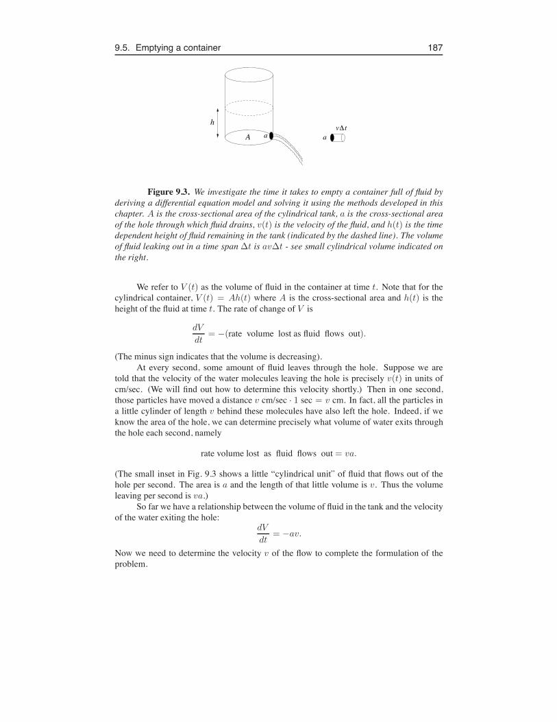
Figure 9.3. We investigate the time it takes to empty a container full of fluid byderiving a differential equation model and solving it using the methods developed in thischapter. A is the cross-sectional area of the cylindrical tank, a is the cross-sectional areaof the hole through which fluid drains, v(t) is the velocity of the fluid, and h(t) is the timedependent height of fluid remaining in the tank (indicated by the dashed line). The volumeof fluid leaking out in a time span !t is av!t - see small cylindrical volume indicated onthe right.

We refer to V (t) as the volume of fluid in the container at time t. Note that for thecylindrical container, V (t) = Ah(t) where A is the cross-sectional area and h(t) is theheight of the fluid at time t. The rate of change of V is

dV

dt= !(rate volume lost as fluid flows out).

(The minus sign indicates that the volume is decreasing).At every second, some amount of fluid leaves through the hole. Suppose we are

told that the velocity of the water molecules leaving the hole is precisely v(t) in units ofcm/sec. (We will find out how to determine this velocity shortly.) Then in one second,those particles have moved a distance v cm/sec · 1 sec = v cm. In fact, all the particles ina little cylinder of length v behind these molecules have also left the hole. Indeed, if weknow the area of the hole, we can determine precisely what volume of water exits throughthe hole each second, namely

rate volume lost as fluid flows out = va.

(The small inset in Fig. 9.3 shows a little “cylindrical unit” of fluid that flows out of thehole per second. The area is a and the length of that little volume is v. Thus the volumeleaving per second is va.)

So far we have a relationship between the volume of fluid in the tank and the velocityof the water exiting the hole:

dV

dt= !av.

Now we need to determine the velocity v of the flow to complete the formulation of theproblem.


9.5.2 Conservation of energyThe fluid “picks up speed” because it has “dropped” by a height h from the top of the fluidsurface to the hole. In doing so, a small mass of water has simply exchanged some potentialenergy (due to its relative height above the hole) for kinetic energy (expressed by how fastit is moving). Potential energy of a small mass of water (m) at height h will be mgh,whereas when the water flows out of the hole, its kinetic energy is given by (1/2)mv2

where v is velocity. Thus, for these to balance (so that total energy is conserved) we have

1

2mv2 = mgh.

(Here v = v(t) is the instantaneous velocity of the fluid leaving the hole and h = h(t) isthe height of the water column.) This allows us to relate the velocity of the fluid leavingthe hole to the height of the water in the tank, i.e.

v2 = 2gh # v =(

2gh. (9.11)

In fact, both the height of fluid and its exit velocity are constantly changing as the fluiddrains, so we might write [v(t)]2 = 2gh(t) or v(t) =

(

2gh(t). We have arrived at thisresult using an energy balance argument.

9.5.3 Putting it togetherWe now combine the various pieces of information to arrive at the model, a differentialequation for a single (unknown) function of time. There are three time-dependent variablesthat were discussed above, the volume V (t), the height h(t), of the velocity v(t). It provesconvenient to express everything in terms of the height of water in the tank, h(t), thoughthis choice is to some extent arbitrary. Keeping units in an equation consistent is essential.Checking for unit consistency can help to uncover errors in equations, including differentialequations.

Recall that the volume of the water in the tank, V (t) is related to the height of fluidh(t) by

V (t) = Ah(t),

where A > 0 is a constant, the cross-sectional area of the tank. We can simplify as follows:

dV

dt=

d(Ah(t))

dt= A

d(h(t))

dt.

But by previous steps and Eqn. (9.11)

dV

dt= !av = !a

(

2gh.

ThusA

d(h(t))

dt= !a

(

2gh,

or simply put,dh

dt= !

a

A

(

2gh = !k&

h. (9.12)

9.5. Emptying a container 189

where k is a constant that depends on the size and shape of the cylinder and its hole:

k =a

A

(

2g.

If the area of the hole is very small relative to the cross-sectional area of the tank, thenk will be very small, so that the tank will drain very slowly (i.e. the rate of change in hper unit time will not be large). On a planet with a very high gravitational force, the sametank will drain more quickly. A taller column of water drains faster. Once its height hasbeen reduced, its rate of draining also slows down. We comment that Equation (9.12) hasa minus sign, signifying that the height of the fluid decreases.

Using simple principles such as conservation of mass and conservation of energy,we have shown that the height h(t) of water in the tank at time t satisfies the differentialequation (9.12). Putting this together with the initial condition (height of fluid h0 at timet = 0), we arrive at initial value problem to solve:

dh

dt= !k

&h, h(0) = h0. (9.13)

Clearly, this equation is valid only for h non-negative. We also remark that Eqn. (9.13) isnonlinear53 as it involves the variable h in a nonlinear term,

&h. Next, we use separation

of variables to find the height as a function of time.

9.5.4 Solution by separation of variablesThe equation (9.13) shows how height of fluid is related to its rate of change, but we areinterested in an explicit formula for fluid height h versus time t. To obtain that relationship,we must determine the solution to this differential equation. We do this using separation ofvariables. (We will also use the initial condition h(0) = h0 that accompanies Eqn. (9.13).)As usual, rewrite the equation in the separated form,

dh&h

= !kdt,

We integrate from t = 0 to t = T , during which the height of fluid that started as h0

becomes some new height h(T ) to be determined." h(T )

h0

1&h

dh = !k

" T

0dt.

Now integrate both sides and simplify:

h1/2

(1/2)

####

h(T )

h0

= !kT

2&(

h(T )!(

h0

'

= !kT

53In many cases, nonlinear differential equations are more challenging than linear ones. However, exampleschosen in this chapter are simple enough that we will not experience the true challenges of such nonlinearities.


(

h(T ) = !kT

2+

(

h0

h(T ) =

$(

h0 ! kT

2

%2

.

Since this is true for any time t, we can also write the form of the solution as

h(t) =

$(

h0 ! kt

2

%2

. (9.14)

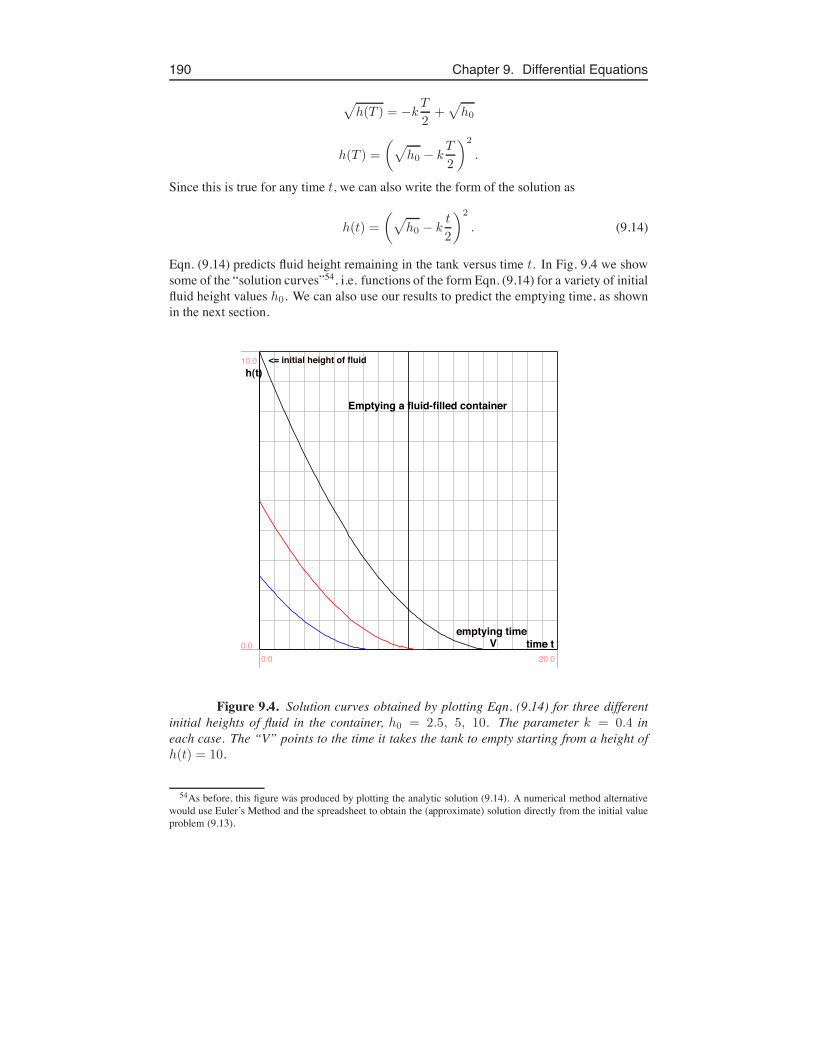
Eqn. (9.14) predicts fluid height remaining in the tank versus time t. In Fig. 9.4 we showsome of the “solution curves”54, i.e. functions of the form Eqn. (9.14) for a variety of initialfluid height values h0. We can also use our results to predict the emptying time, as shownin the next section.

h(t)

time t

<= initial height of fluid

emptying timeV

Emptying a fluid-filled container

0.0 20.00.0

10.0

Figure 9.4. Solution curves obtained by plotting Eqn. (9.14) for three differentinitial heights of fluid in the container, h0 = 2.5, 5, 10. The parameter k = 0.4 ineach case. The “V” points to the time it takes the tank to empty starting from a height ofh(t) = 10.

54As before, this figure was produced by plotting the analytic solution (9.14). A numerical method alternativewould use Euler’s Method and the spreadsheet to obtain the (approximate) solution directly from the initial valueproblem (9.13).

9.6. Density dependent growth 191

9.5.5 How long will it take the tank to empty?The tank will be empty when the height of fluid is zero. Setting h(t) = 0 in Eqn. 9.14

$(

h0 ! kt

2

%2

= 0.

Solving this equation for the emptying time te, we get

kte2

=(

h0 # te =2&

h0

k.

The time it takes to empty the tank depends on the initial height of water in the tank. Threeexamples are shown in Figure 9.4 for initial heights of h0 = 2.5, 5, 10. The emptying timedepends on the square-root of the initial height. This means, for instance, that doubling theheight of fluid initially in the tank only increases the time it takes by a factor of

&2 ' 1.41.

Making the hole smaller has a more direct “proportional” effect, since we have found thatk = (a/A)

&2g.

9.6 Density dependent growthThe simple model discussed in Section 9.2 for population growth has an unrealistic featureof unlimited explosive exponential growth. To correct for this unrealistic feature, a commonassumption is that the rate of growth is “density dependent”. In this section, we considera revised differential equation that describes such growth, and use the new tools to analyzeits predictions. In place of our previous notation we will now use N to represent the sizeof a population.

9.6.1 The logistic equationThe logistic equation is the simplest density dependent growth equation, and we study itsbehaviour below.

Let N(t) be the size of a population at time t. Clearly, we expect N(t) $ 0 for alltime t, since a population cannot be negative. We will assume that the initial population isknown, N(0) = N0. The logistic differential equation states that the rate of change of thepopulation is given by

dN

dt= rN

$K ! N

K

%

. (9.15)

Here r > 0 is called the intrinsic growth rate and K > 0 is called the carrying capacity.K reflects that size of the population that can be sustained by the given environment. Wecan understand this equation as a modified growth law in which the “density dependent”term, r(K ! N)/K , replaces the previous constant net growth rate k.


9.6.2 Scaling the equationThe form of the equation can be simplified if we measure the population in units of thecarrying capacity, instead of “numbers of individuals”. i.e. if we define a new quantity

y(t) =N(t)

K.

This procedure is called scaling. To see this, consider dividing each side of the logisticequation (9.15) by the constant K . Then

1

K

dN

dt=

r

KN

$K ! N

K

%

.

We now group terms conveniently, forming

d(NK )

dt= r

$N

K

% $

1 !$

N

K

%%

.

Replacing (N/K) by y in each case, we obtain the scaled equation and initial conditiongiven by

dy

dt= ry(1 ! y), y(0) = y0. (9.16)

Now the variable y(t) measures population size in “units” of the carrying capacity, andy0 = N0/K is the scaled initial population level. Here again is an initial value problem,like Eqn. (9.13), but unlike Eqn. (9.1), the logistic differential equation is nonlinear. Thatis, the variable y appears in a nonlinear expression (in fact a quadratic) in the equation.

9.6.3 Separation of variablesHere we will solve Eqn. (9.16) by separation of variables. The idea is essentially the sameas our previous examples, but is somewhat more involved. To show an alternative methodof handling the integration, we will treat both sides as indefinite integrals. Separating thevariables leads to

1

y(1 ! y)dy = r dt

"1

y(1 ! y)dy =

"

r dt + K.

The integral on the right will lead to rt + K where K is some constant of integration thatwe need to incorporate since we do not have endpoints on our integrals. But we must workharder to evaluate the integral on the left. We can do so by partial fractions, the techniquedescribed in Section 6.6. Details are given in Section 9.6.4.

9.6.4 Application of partial fractionsLet

I =

"1

y(1 ! y)dy.

9.6. Density dependent growth 193

Then for some constants A, B we can write

I =

"A

y+

B

1 ! ydy = A ln |y|! B ln |1 ! y|.

(The minus sign in front of B stems from the fact that letting u = 1 ! y would lead todu = !dy.) We can find A, B from the fact that

A

y+

B

1 ! y=

1

y(1 ! y),

so thatA(1 ! y) + By = 1.

This must be true for all y, and in particular, substituting in y = 0 and y = 1 leads toA = 1, B = 1 so that

I = ln |y|! ln |1 ! y| = ln

####

y

1 ! y

####.

9.6.5 The solution of the logistic equationWe now have to extract the quantity y from the equation

$

ln

####

y

1 ! y

####

%

= rt + K.

That is, we want y as a function of t. After exponentiating both sides we need to removethe absolute value. We will now assume that y is initially smaller than 1, and show that itremains so. In that case, everything inside the absolute value is positive, and we can write

y(t)

(1 ! y(t))= ert+K = eKert = Cert.

In the above step, we have simply renamed the constant, eK by the new name C for sim-plicity. C > 0 is now also an arbitrary constant whose value will be determined from theinitial conditions. Indeed, if we substitute t = 0 into the most recent equation, we find that

y(0)

(1 ! y(0))= Ce0 = C,

so thatC =

y0

(1 ! y0).

We will use this fact shortly. What remains now is some algebra to isolate the desiredfunction y(t)

y(t) = (1 ! y(t))Cert.

y(t))

1 + Cert*

= Cert.


y(t) =Cert

(1 + Cert)=

1

(1/C)e!rt + 1.

The desired function is now expressed in terms of the time t, and the constants r, C. Wecan also express it in terms of the initial value of y, i.e. y0, by using what we know to betrue about the constant C, i.e. C = y0/(1 ! y0). When we do so, we arrive at

y(t) =1

1+y0

y0e!rt + 1

=y0

(y0 + (1 ! y0)e!rt). (9.17)

Some typical solution curves of the logistic equation are shown in Fig. 9.5.

y(t)

time t

Solutions to Logistic equation

0.0 30.00.0

1.0

Figure 9.5. Solution curves for y(t) in the scaled form of the logistic equationbased on (9.18). We show the predicted behaviour of y(t) as given by Eqn. (9.17) for threedifferent initial conditions, y0 = 0.1, 0.25, 0.5. Note that all solutions approach the valuey = 1.

9.6.6 What this solution tells usWe have arrived at the function that describes the scaled population as a function of timeas predicted by the scaled logistic equation, (9.16). The level of population (in units of thecarrying capacity K) follows the time-dependent function

y(t) =y0

(y0 + (1 ! y0)e!rt). (9.18)

9.7. Extensions and other population models: the “Law of Mortality” 195

We can convert this result to an equivalent expression for the unscaled total population N(t)by recalling that y(t) = N(t)/K . Substituting this for y(t), and noting that y0 = N0/Kleads to

N(t) =N0

(N0 + (K ! N0)e!rt). (9.19)

It is left as an exercise for the reader to check this claim.Now recall that r > 0. This means that e!rt is a decreasing function of time. There-

fore, (9.18) implies that, after a long time, the term e!rt in the denominator will be negli-gibly small, and so

y(t) %y0

y0= 1,

so that y will approach the value 1. This means that

(N/K) % 1 or simply N(t) % K.

The population will thus settle into a constant level, i.e., a steady state, at which no furtherchange will occur.

As an aside, we observe that this too, could have been predicted directly from thedifferential equation. By setting dy/dt = 0, we find that

0 = ry(1 ! y),

which suggests that y = 1 is a steady state. (This is also true for the less interesting caseof no population, i.e. y = 0 is also a steady state.) Similarly, this could have been foundby setting the derivative to zero in Eqn. (9.15), the original, unscaled logistic differentialequation. Doing so leads to

dN

dt= 0 # rN

$K ! N

K

%

= 0.

If r > 0, the only values of N satisfying this steady state equation are N = 0 or N =K . This implies that either N = 0 or N = K are steady states. The former is not toointeresting. It states the obvious fact that if there is no population, then there can be nopopulation growth. The latter reflects that N = K , the carrying capacity, is the populationsize that will be sustained by the environment.

In summary, we have shown that the behaviour of the logistic equation for populationgrowth is more realistic than the simpler exponential growth we studied earlier. We sawin Figure 9.5, that a small population will grow, but only up to some constant level (thecarrying capacity). Integration, and in particular the use of partial fractions allowed us tomake a full prediction of the behaviour of the population level as a function of time, givenby Eqn. (9.19).

9.7 Extensions and other population models: the“Law of Mortality”

There are many variants of the logistic model that are used to investigate the growth ormortality of a population. Here we extend tools to another example, the gradual decline of


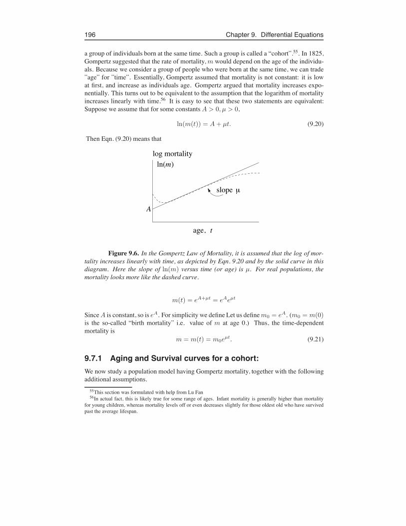
a group of individuals born at the same time. Such a group is called a “cohort”.55. In 1825,Gompertz suggested that the rate of mortality, m would depend on the age of the individu-als. Because we consider a group of people who were born at the same time, we can trade”age” for ”time”. Essentially, Gompertz assumed that mortality is not constant: it is lowat first, and increase as individuals age. Gompertz argued that mortality increases expo-nentially. This turns out to be equivalent to the assumption that the logarithm of mortalityincreases linearly with time.56 It is easy to see that these two statements are equivalent:Suppose we assume that for some constants A > 0, µ > 0,

ln(m(t)) = A + µt. (9.20)

Then Eqn. (9.20) means that

t

ln( )m

A

slope µ

log mortality

age,

Figure 9.6. In the Gompertz Law of Mortality, it is assumed that the log of mor-tality increases linearly with time, as depicted by Eqn. 9.20 and by the solid curve in thisdiagram. Here the slope of ln(m) versus time (or age) is µ. For real populations, themortality looks more like the dashed curve.

m(t) = eA+µt = eAeµt

Since A is constant, so is eA. For simplicity we define Let us define m0 = eA. (m0 = m(0)is the so-called “birth mortality” i.e. value of m at age 0.) Thus, the time-dependentmortality is

m = m(t) = m0eµt. (9.21)

9.7.1 Aging and Survival curves for a cohort:We now study a population model having Gompertz mortality, together with the followingadditional assumptions.

55This section was formulated with help from Lu Fan56In actual fact, this is likely true for some range of ages. Infant mortality is generally higher than mortality

for young children, whereas mortality levels off or even decreases slightly for those oldest old who have survivedpast the average lifespan.

9.8. Summary 197

1. All individuals are assumed to be identical.

2. There is “natural” mortality, but no other type of removal. This means we ignore themortality caused by epidemics, by violence and by wars.

3. We consider a single cohort, and assume that no new individuals are introduced (e.g.by immigration)57.

We will now study the size of a “cohort”, i.e. a group of people who were born in the sameyear. We will denote by N(t) the number of people in this group who are alive at time t,where t is time since birth, i.e. age. Let N(0) = N0 be the initial number of individuals inthe cohort.

9.7.2 Gompertz ModelAll the people in the cohort were born at time (age) t = 0, and there were N0 of them atthat time. That number changes with time due to mortality. Indeed,

The rate of change of cohort size = ![number of deaths per unit time]= ![mortality rate] · [cohort size]

Translating to mathematical notation, we arrive at the differential equation

dN(t)

dt= !m(t)N(t),

and using information about the size of the cohort at birth leads to the initial condition,N(0) = N0. Together, this leads to the initial value problem

dN(t)

dt= !m(t)N(t), N(0) = N0.

Note similarity to Eqn. (9.1), but now mortality is time-dependent.In the Problem set, we apply separation of variables and integrate over the time in-

terval [0, T ]: to show that the remaining population at age t is

N(t) = N0e!

m0µ (eµt

!1).

9.8 SummaryIn this chapter, we used integration methods to find the analytical solutions to a variety ofdifferential equations where initial values were prescribed.

We investigated a number of population growthmodels:

1. Exponential growth, given by dydt = ky, with initial population level y(0) = y0

was investigated (Eqn. (9.1)). This model had an unrealistic feature that growth isunlimited.

57Note that new births would contribute to other cohorts.


2. The Logistic equation dNdt = rN

)K!N

K

*

was analyzed (Eqn. (9.15)), showing thatdensity-dependent growth can correct for the above unrealistic feature.

3. The Gompertz equation, dN(t)dt = !m(t)N(t), was solved to understand how age-

dependent mortality affects a cohort of individuals.

In each of these cases, we used separation of variables to “integrate” the differentialequation, and predict the population as a function of time.

We also investigated several other physical models in this chapter, including thevelocity of a falling object subject to drag force. This led us to study a differential equationof the form dy

dt = a ! by. By slight reinterpretation of terms in this equation, we can useresults to understand chemical kinetics and blood alcohol levels, as well as a host of otherscientific applications.

Section 9.5, the “centerpiece” of this chapter, illustrated the detailed steps that go intothe formulation of a differential equation model for flow of liquid out of a container. Herewe saw how conservation statements and simplifying assumptions are interpreted together,to arrive at a differential equation model. Such ideas occur in many scientific problems, inchemistry, physics, and biology.

Documents

Chapter 9 Differential Equations - Undergrad · PDF fileChapter 9 Differential Equations 9.1 Introduction A differential equation is a relationship between some (unknown) function