Embed Size (px)
Citation preview

Chapter 9: Bayesian Methods
CS 336/436
Gregory D. Hager


A Simple
Example

Why Not Just Use a Kalman Filter?
Recall Robot Localization
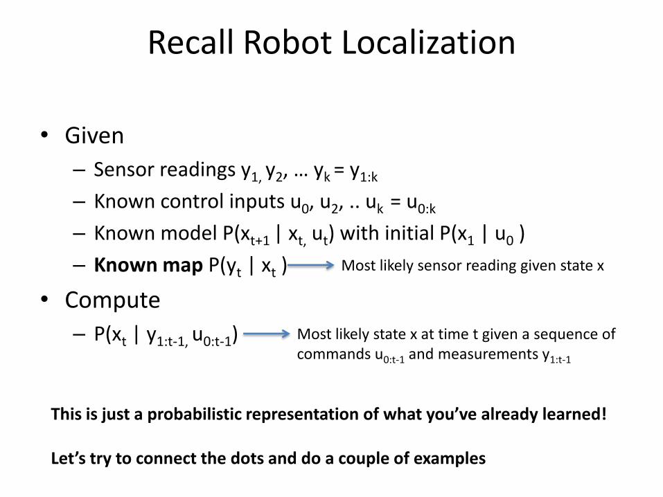
• Given
– Sensor readings y1, y2, … yk = y1:k
– Known control inputs u0, u2, .. uk = u0:k
– Known model P(xt+1 | xt, ut) with initial P(x1 | u0 )
– Known map P(yt | xt )
• Compute
– P(xt | y1:t-1, u0:t-1)
This is just a probabilistic representation of what you’ve already learned! Let’s try to connect the dots and do a couple of examples
Most likely sensor reading given state x
Most likely state x at time t given a sequence of commands u0:t-1 and measurements y1:t-1

Some Probability Reminders
• P(x,y) = P(x | y) P(y)
• P(x) = y P(x, y) = y P(x | y) P(y)
• If x is independent of z given y
– P(x | y, z) = P(x | y)
• Two important assumptions
1. Markov
2. Observation
ò ò
wikipedia
P(X) P(Y)
)|(),,|( 101 kkkk xxPxxxP
)|(),,|( 0 kkkk xyPxxyP

Bayes Filter • Given a sequence of measurements y1, …, yk and a
sequence of commands u0, …, uk-1: { y1:k, u0:k-1 }
• Given a sensor model P( yk | xk )
• Given a dynamic model P( xk | xk-1 )
• Given a prior probability P(x0)
Find P(xk | y1:k, u0:k-1 )
x0 xk-2 xk-1 xk
yk-2 yk-1 yk
u0 uk-2 uk-1

Bayesian Localization
• Recall Bayes Theorem:
P(x | y ) = P(y | x) P(x)/ P(y)
• Also remember conditional independence
• Think of x as the state of the robot and y as the data we know
P(xk | u0:k-1, y1:k ) Posterior Probability Distribution
P(xk | u0:k-1, y1:k ) = P(yk | xk, u0:k-1, y1:k-1) P(xk | u0:k-1, y1:k-1) / P(yk | u0:k-1, y1:k-1)
= hk P(yk | xk) xk-1 P(xk | uk-1, xk-1) P(xk-1 | u0:k-2, y1:k-1 )
observation recursive instance state prediction

A Simple
Example

Ways of Representing Probabilities
• We have already seen Kalman filters – represent probabilities as Gaussians – Gaussians are conjugate distributions
• How arbitrary distributions are represented? – Mixtures of Gaussians
• Suppose instead state space is partitioned and probability in partition is constant – P(x | y ) = P(y | x) P(x) / P(y) P(xi | y) = h P(y | xi) P(xi) – h = i P(y | xi) P(xi) – Thus, updating from observations is a simple multiplication of prior probability by likelihood of
observation
– P(xi(k) | u(k-1:0), y(k-1)) = j P(xi(k) | u(k-1), xj(k-1)) P(xj(k-1) | u(k-2:0), y(k-1))
– Thus, updating using dynamical model is simply a discrete convolution (blurring) of the prior by the driving noise of the planned motion
http://arxiv.org/pdf/1304.2757.pdf A blast from the past:

How Do We Think about Motion?
• Suppose we have P(xk)
• We have P(xk+1 | xk, uk)
• Put together
• P(xk+1) = P(xk+1 | xk, uk) P(xk) dxk
What is the probability distribution for xk+1 given the command uk and all the previous states xk?
ò
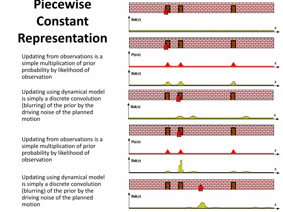
Piecewise Constant
Representation Updating from observations is a simple multiplication of prior probability by likelihood of observation
Updating using dynamical model is simply a discrete convolution (blurring) of the prior by the driving noise of the planned motion
Updating from observations is a simple multiplication of prior probability by likelihood of observation
Updating using dynamical model is simply a discrete convolution (blurring) of the prior by the driving noise of the planned motion

Piecewise Constant Representation (Mobile Robot)
),,( >=< qyxxBel t
Position of a mobile robot: (x, y, q)
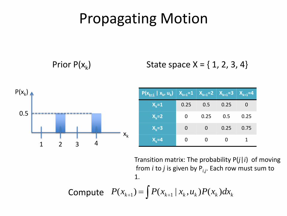
Propagating Motion
State space X = { 1, 2, 3, 4}
P(xk+1 | xk, uk) Xk+1=1 Xk+1=2 Xk+1=3 Xk+1=4
Xk=1 0.25 0.5 0.25 0
Xk=2 0 0.25 0.5 0.25
Xk=3 0 0 0.25 0.75
Xk=4 0 0 0 1 xk
P(xk)
1 2 3 4
0.5
kkkkkk dxxPuxxPxP )(),|()( 11
Prior P(xk)
Compute
Transition matrix: The probability P(j|i) of moving from i to j is given by Pi,j. Each row must sum to 1.
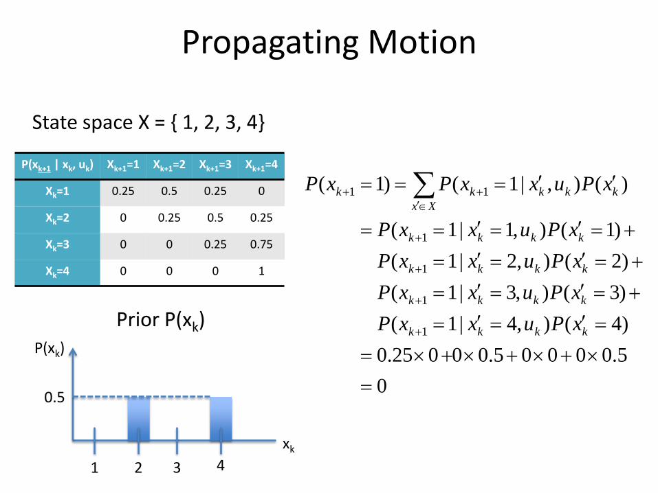
Propagating Motion
State space X = { 1, 2, 3, 4}
P(xk+1 | xk, uk) Xk+1=1 Xk+1=2 Xk+1=3 Xk+1=4
Xk=1 0.25 0.5 0.25 0
Xk=2 0 0.25 0.5 0.25
Xk=3 0 0 0.25 0.75
Xk=4 0 0 0 1
xk
P(xk)
1 2 3 4
0.5
Prior P(xk)
0
5.00005.00025.0
)4(),4|1(
)3(),3|1(
)2(),2|1(
)1(),1|1(
)(),|1()1(
1
1
1
1
11
kkkk
kkkk
kkkk
kkkk
Xx
kkkkk
xPuxxP
xPuxxP
xPuxxP
xPuxxP
xPuxxPxP

Propagating Motion
State space X = { 1, 2, 3, 4}
P(xk+1 | xk, uk) Xk+1=1 Xk+1=2 Xk+1=3 Xk+1=4
Xk=1 0.25 0.5 0.25 0
Xk=2 0 0.25 0.5 0.25
Xk=3 0 0 0.25 0.75
Xk=4 0 0 0 1
xk
P(xk)
1 2 3 4
0.5
Prior P(xk)
125.0
5.00005.025.005.0
)4(),4|2(
)3(),3|2(
)2(),2|2(
)1(),1|2(
)(),|2()2(
1
1
1
1
11
kkkk
kkkk
kkkk
kkkk
Xx
kkkkk
xPuxxP
xPuxxP
xPuxxP
xPuxxP
xPuxxPxP

Propagating Motion
State space X = { 1, 2, 3, 4}
P(xk+1 | xk, uk) Xk+1=1 Xk+1=2 Xk+1=3 Xk+1=4
Xk=1 0.25 0.5 0.25 0
Xk=2 0 0.25 0.5 0.25
Xk=3 0 0 0.25 0.75
Xk=4 0 0 0 1
xk
P(xk)
1 2 3 4
0.5
Prior P(xk)
25.0
5.00025.05.05.0025.0
)4(),4|3(
)3(),3|3(
)2(),2|3(
)1(),1|3(
)(),|3()3(
1
1
1
1
11
kkkk
kkkk
kkkk
kkkk
Xx
kkkkk
xPuxxP
xPuxxP
xPuxxP
xPuxxP
xPuxxPxP

Propagating Motion
State space X = { 1, 2, 3, 4}
P(xk+1 | xk, uk) Xk+1=1 Xk+1=2 Xk+1=3 Xk+1=4
Xk=1 0.25 0.5 0.25 0
Xk=2 0 0.25 0.5 0.25
Xk=3 0 0 0.25 0.75
Xk=4 0 0 0 1
xk
P(xk)
1 2 3 4
0.5
Prior P(xk)
625.0
5.01075.05.025.000
)4(),4|4(
)3(),3|4(
)2(),2|4(
)1(),1|4(
)(),|4()4(
1
1
1
1
11
kkkk
kkkk
kkkk
kkkk
Xx
kkkkk
xPuxxP
xPuxxP
xPuxxP
xPuxxP
xPuxxPxP
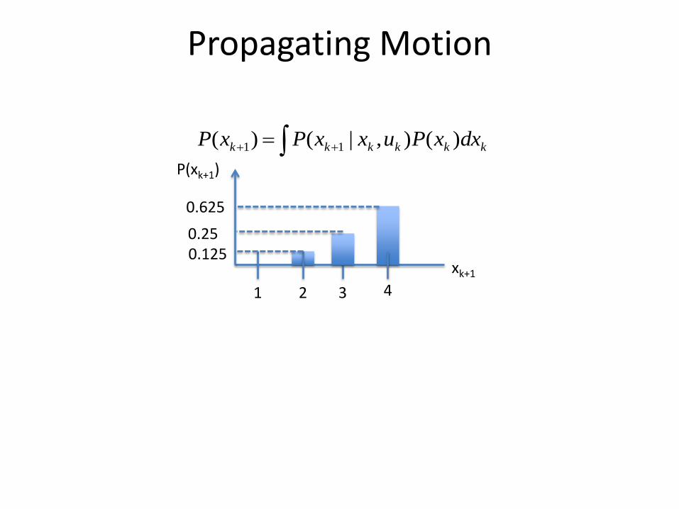
Propagating Motion
xk+1
P(xk+1)
1 2 3 4
0.625
kkkkkk dxxPuxxPxP )(),|()( 11
0.25 0.125

Discrete Bayes Filter Algorithm Algorithm Discrete_Bayes_filter( u0:k-1, y1:k, P(x0) )
1. P(x) = P(x0)
2. for i=1:k
3. for all states x X
4.
5. end for
6. h=0
7. for all states x X
8.
9. h = h + P(x)
10. end for
11. for all states x X
12. P(x) = P(x) / h
13. end for
14. end for
Xx
i xPxuxPxP )(),|()( 1
)()|()( xPxyPxP i
Prediction given prior dist. and command
Update using measurement
Normalize to 1

Note About the Posterior
• It is a probability distribution
• What do we do with it?
– Maximum likelihood:
– Mean Squared Error:
x
P(x)
]))ˆ()([( 2xPxPE
)|(maxarg xzPx

Bayes Filter Ingredients
• Motion model
P( xk | xk-1, uk-1 )
• Observation model
P( yk | xk )
• Bayes estimator
MAP, MSE,

How To Get Likelihoods?
• How do we get p(y | x)?
• In the discrete case, x is a fixed value
• For a fixed value and *known* map, we can predict/simulate sensor readings y* (recall y = h(x) + v)
• But, we know y* - y ~ v for whatever distribution v has – v is Gaussian with covariance L, then P(y | x) = G(y*-y ; 0, L)
– v could be represented with an empirical histogram; P(y | x) is a table lookup

Grid-based Localization

Sonars and Occupancy Grid Map

Localization Algorithms - Comparison
Kalman filter Multi-hypothesis
tracking
Grid-based
(fixed/variable)
Sensors Gaussian Gaussian Non-Gaussian
Posterior Gaussian Multi-modal Piecewise constant
Efficiency (memory) ++ ++ -/+
Efficiency (time) ++ ++ o/+
Implementation + o +/o
Accuracy ++ ++ +/++
Robustness - + ++
Global localization No Yes Yes

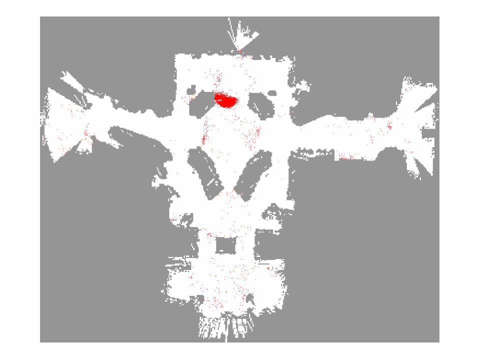
Represent belief by random samples
Estimation of non-Gaussian, nonlinear processes
Monte Carlo filter, Survival of the fittest,
Condensation, Bootstrap filter, Particle filter
Filtering: [Rubin, 88], [Gordon et al., 93], [Kitagawa 96]
Computer vision: [Isard and Blake 96, 98]
Dynamic Bayesian Networks: [Kanazawa et al., 95]d
Particle Filters

Sample-based Density Representation

draw xit1 from Bel(xt1)
draw xit from p(xt | x
it1,ut1)
Importance factor for xit:
)|(
)(),|(
)(),|()|(
ondistributi proposal
ondistributitarget
111
111
tt
tttt
tttttt
i
t
xzp
xBeluxxp
xBeluxxpxzp
w
µ
=
=
---
---h
1111 )(),|()|()( ----ò= tttttttt dxxBeluxxpxzpxBel h
Particle Filter Algorithm

Monte Carlo Localization
• Monte-Carlo-Localization(a, z, N, map) – S = N samples from P(X(t)) from previous call
– for i = 1 to N • S[i] = sample from P(X(t+1) | X(t) = S[i], A = a)
• W[i] = 1
• for j = 1 to M do
– z* = expected-sensor-reading(j,S[i],map)
– W[i] = W[i] * P(Z = z(j) | Z* = Z*)
– S = weighted-sample-with-replacement(N, S, W)
– return S
• Note that S is a discrete representation of the probability of robot location

The Likehihood Function
• Generating the sensor likelihood is essentially a sensor simulation
– can be expensive
– pre-compute
– approximate
• A good fast approximation is often a weighted sum of
– a nominal model that is fast to compute
– other deviations that are modeled as random elements

Proximity Sensor Model
Laser sensor Sonar sensor
Tuned model that takes into account normal reflection, unexpected returns and randomness and out of range
Resampling
• Given: Set S of weighted samples.
• Wanted : Random sample, where the probability of drawing xi is given by wi.
• Typically done n times with replacement to generate new sample set S’.
w2
w3
w1 wn
Wn-1
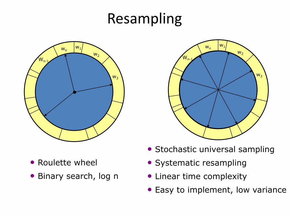
Resampling
w2
w3
w1 wn
Wn-1
• Roulette wheel
• Binary search, log n
• Stochastic universal sampling
• Systematic resampling
• Linear time complexity
• Easy to implement, low variance

1. Algorithm systematic_resampling(S,n):
2.
3. For Generate cdf
4.
5. Initialize threshold
6. For Draw samples …
7. While ( ) Skip until next threshold reached
8.
9. Insert
10. Increment threshold
11. Return S’
Resampling Algorithm
1
1,' wcS =Æ=
ni …2=i
ii wcc += -1
u1 ~U[0,1 / n], i = 1
nj …1=
u j = u j +1 / n
ij cu >
S ' = S 'È < xi ,1 / n >{ }1+= ii
Also called stochastic universal sampling

Start
Motion Model Reminder

Sample-based Localization (sonar)


Using Ceiling Maps for Localization
[Dellaert et al. 99]

Ceiling Light Localization

Vision-based Localization
P(z|x)
h(x)
z

Under a Light
Measurement z: P(z|x):

Next to a Light
Measurement z: P(z|x):

Elsewhere
Measurement z: P(z|x):

Sample-based Localization Demos
http://www.cs.washington.edu/ai/Mobile_Robotics//mcl/
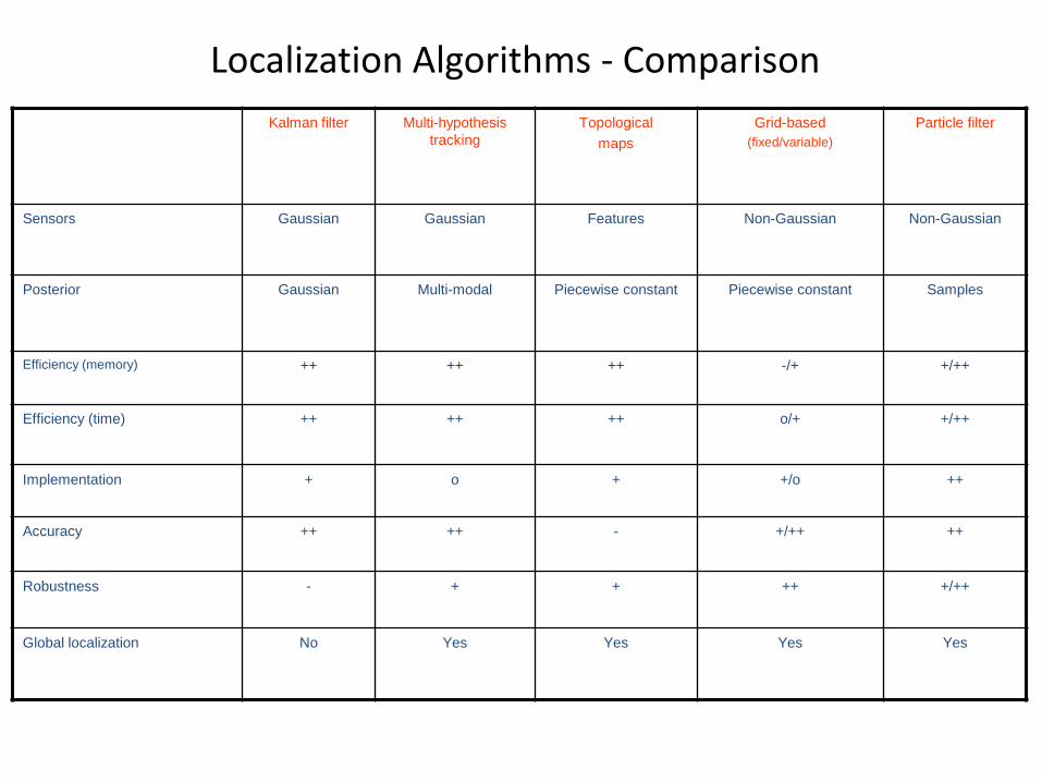
Localization Algorithms - Comparison
Kalman filter Multi-hypothesis
tracking
Topological
maps
Grid-based
(fixed/variable)
Particle filter
Sensors Gaussian Gaussian Features Non-Gaussian Non-Gaussian
Posterior Gaussian Multi-modal Piecewise constant Piecewise constant Samples
Efficiency (memory) ++ ++ ++ -/+ +/++
Efficiency (time) ++ ++ ++ o/+ +/++
Implementation + o + +/o ++
Accuracy ++ ++ - +/++ ++
Robustness - + + ++ +/++
Global localization No Yes Yes Yes Yes

Bayes Filters for Robot Localization
Arbitrary posteriors
Exponential in state dimensions Global localization
Optimal, converges to true posterior Non-linear dynamics/observations
Sample-based approximation
Arbitrary posteriors
Exponential in state dimensions Global localization
Optimal, converges to true posterior Non-linear dynamics/observations
Piecewise constant approximation
Extended / unscented
First and second moment
Position tracking
Kalman filter
Non-linear dynamics/observ.
Quadratic in state dimension
Linear dynamics/observations
Position tracking
Polynomial in state dimension
Multi-modal Gaussian
Not optimal (linear approx.)
Global localization
Non-linear dynamics/observations
Grid
Particle filter
Discrete
Bayes filters
Not optimal (linear approx.)
Continuous
fixed/variable resolution Kalman filter
Multi-hypothesis
Abstract dynamics/observations
Abstract state space
Topological
Global localization One-dimensional graph
Arbitrary, discrete posteriors First and second moment
Optimal (linear, Gaussian)
tracking (EKF)
Quadratic in state dimension

Some Maps

Problems in Mapping
• Sensor interpretation
– How do we extract relevant information from raw sensor data?
– How do we represent and integrate this information over time?
– Do we map for the purpose of localization or do we map for “human consumption” (dense vs sparse)?
• Robot locations have to be known
– How can we estimate them during mapping?

Occupancy Grid Maps
• Introduced by Moravec and Elfes in 1985
• Represent environment by a grid.
• Estimate the probability that a location is occupied by an obstacle.
• Key assumptions – Occupancy of individual cells is
independent
– Robot positions x(1:k) are known!
Bel(mt ) = P(mt | x(1 : k), y(1 : k))
= Bel(mt[xy] | x(1 : k), y(1 : k))
x,y
Õ
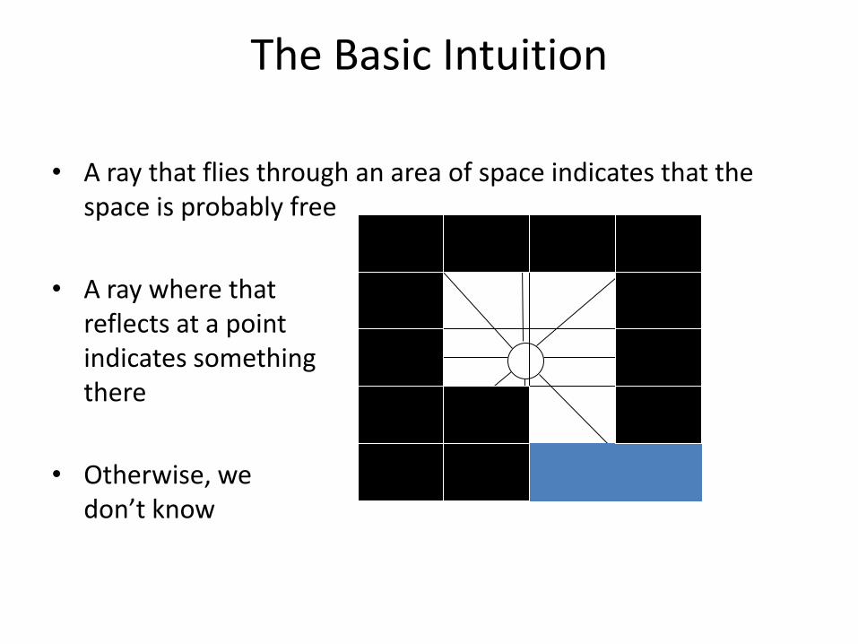
The Basic Intuition
• A ray that flies through an area of space indicates that the space is probably free
• A ray where that reflects at a point indicates something there
• Otherwise, we don’t know

One Idea: Simple Counting
• For every cell count – hits(x,y): number of cases where a beam ended at <x,y> – misses(x,y): number of cases where a beam passed
through <x,y>
• Assumption: P(occupied(x,y)) = P(reflects(x,y))
• Many cases where this is not a good approximation … e.g. sonar reflection model
),misses(),hits(
),hits()( ][
yxyx
yxmBel xy
+=

Updating Occupancy Grid Maps
• Note that the following also can be derived:
• Now, consider the odds ratio:
P(Øm[xy] | x(1 : k), y(1 : k)) =
P(Øm[xy] | y(k), x(k))P(y(k) | x(k))P(Øm[xy] | x(1 : k -1), y(1 : k -1))
O(m[xy] | x(1 : k), y(1 : k)) =
hO(m[xy] | y(k), x(k))O(m[xy] | x(1 : k -1), y(1 : k -1))
inverse sensor model Prior odds
)(
)(
)(1
)()(
xP
xP
xP
xPxOdds

Updating Occupancy Grid Maps
• Typically updated using inverse sensor model and log odds ratio (log ab = log a + log b)
and then recover the probability with
1
)(
11)(
xOddsxP
hlog))1:1(),1:1(|(log))(),(|(log)):1(),:1(|(log kykxmOkykxmOkykxmO
1
)1:1(),1:1(|(
)1:1(),1:1(|(1
1)(),(|(
))(),(|(11)):1(),:1(|(
kykxmP
kykxmP
kykxmP
kykxmPkykxmP
h
h

The Inverse Sensor Model
• The probability a cell is occupied given observation and localization
Assume that all cells are independent
then specify , which is the probability of cell ml is occupied given the measurement y(k) in position x(k)
))(),(|( kykxmP
l
lmPmP )()(
))(),(|( kykxmP l

Learning Inverse Sensor Model
• Learn probabilities with neural network.
• Consider four beams simultaneously.
[Thrun ’98]

Occupancy Grid Algorithm
Algorithm Occupancy_grid( x1:k, y1:k, P0(m) ):
1. Pm = P0(m)
2. for i=1 to k
3.
1
1
1)(),(|(
))(),(|(11
m
mm
P
P
kykxmP
kykxmPP
h
h

Occupancy Grids: From scans to maps

Tech Museum, San Jose
CAD map occupancy grid map

Concurrent Mapping and Localization
• Chicken-and-egg problem – Mapping with known poses is “simple”
– Localization with known map is “simple”
– But in combination the problem is hard!
70 m

Mapping with Expectation Maximization
• Idea: Maximum likelihood with unknown data association.
Bel(m, x(k)) º P(x(1: k),m |u(0 : k -1), y(1: k))
Bel(m, x(k)) =h p(y(k) |m, x(k)) p(x(k) | x(k -1),u(k -1))Bel(m, x(k -1))ò dxt-1
m[k+1] = argmaxm
Q [x(1 : k) |m[k ]]
Q[x(1: k) |m[k ]] = Em[ k ] [log p(x(1: k) |m[k ],u(0 : k -1), y(1: k))]E-step:
M-step:
Mapping with known poses
Localization (bi-directional)
• EM: Maximize log-likelihood by iterating
Take this apart: first estimate location given map, then estimate map given location

EM Mapping, Example (width 45 m)

CSIRO

SLAM
• Idea: Given the true trajectory of the robot, all landmark detections are independent. – The first term is “easy” (mapping given location and data) – The second term is “easy” (predict location from prior data) – The “hard” part: we know have to represent distributions on
*trajectories*!
• We can use Rao-Blackwellised particle filters to estimate robot
locations and landmark locations. (FastSLAM, Montemerlo)
• Update can be done efficiently (O(m log n)).
P(x(1:k),m | u(0:k-1),y(1:k)) = P(m | x(1:k), y(1:k), u(0:k-1)) P(x(1:k) | y(1:k) u(0:k-1)) = P(m | x(1:k),y(1:k)) P(x(1:k) | y(1:k),u(0:k-1))

Sufficient Statistic
• A statistic is a function T(X1,X2,…Xn) of the random samples X1,X2,…,Xn
Examples:
n
i
iXn
X1
1
n
i
i XXn
s1
22
1
1
nXXXT ,...,,max 21

Sufficient Statistic
• Given X1,X2,…,Xn, is there a small set of statistics that can contain all the information about the samples?
• If fq(x) is a probability distribution (q is parameter), then T is a sufficient statistic for q if we can factorize
• If T is a sufficient statistic then it contain all the information to compute an estimate of q
))(()()( xTgxhxf qq Function of the statistic
Not a function of q

Sufficient Statistic
• Given X1,X2,…,Xn, is there a statistic that can contain all the information about the samples?
– Poisson distribution: • X1,X2,…,Xn are independent samples from a Poisson distribution
with parameter l. Then a sufficient statistic T(X) of l is
• Note that T(X) does not depend on l
n
i
iXXT1
)(

Sufficient Statistic
• Given X1,X2,…,Xn, is there a statistic that can contain all the information about the samples?
– Exponential distribution: • X1,X2,…,Xn are independent and exponentially distributed with
expected value l. Then a sufficient statistic T(X) of l is
• Note that T(X) does not depend on l
n
i
iXXT1
)(

Rao-Blackwell Theorem
• Improve the efficiency of an estimator by taking its conditional expectation with respect to a sufficient statistic – Estimator : Is a statistic (rule) used to estimate an
unobservable parameter q in a population • The average of N random samples is an estimator of the
population’s average (i.e. height)
– Sufficient statistic T(X): Given T(X), the distribution of observable samples X does not depends on the unobservable parameter q
– Rao Blackwell estimator of q is defined by
and has better mean squared error than
)(ˆ Xq
)](|)(ˆ[)(ˆ XTXEXR qq
)(ˆ Xq

What About SLAM?
• Recall the Bayes filtering problem. The posterior satisfies the recursion
where zk is hidden (put up with “z” instead of “x” for now)
• That integral is often not tractable and numeric approximations with samples is often used
)|()|()|()|( 1:11:01:1:0
1
kk
z
kkkkkkk yzPzzPzyPyzP
k
h

Marginalize the State Space in Two
• Suppose we can divide zk in two groups: xk and mk such that P(zk|zk-1) = P(mk|xk-1:k, mk-1)P(xk|xk-1) and assume that P(m0:k|y1:k, x0:k) is tractable
• Then we can marginalize x0:k from the posterior and focus on estimating P(x0:k |y1:k ) which is a “smaller” problem. Essentially we convert the problem to
P(x0:k, m0:k | y1:k) = P(m0:k|y1:k, x0:k) P(x0:k|y1:k)
Optimal Filt. Particle Filt.
and the posterior distribution of P(x0:k|y1:k) is given
The dimension of P(x0:k|y1:k) is smaller than P(x0:k, m0:k | y1:k)
1
)|()|()|()|( 1:11:01:1:0
kx
kkkkkkkkk yxPxxPxyPnyxP

Rao-Blackwellized SLAM
),|,( 1:0:1:1 kkk uymxp
),|(),,|( 1:0:1:11:0:1:1 kkktkk uyxpuyxmp
Compute a posterior over the map and possible trajectories of the robot :
robot motion map trajectory
map and trajectory
measurements
Begin Courtesy Dieter Fox
mapping Localization

m
x
y
u
x
y
u
2
2
x
y
u
... t
t
x 1
1
0
1 0 t-1
A Graphical Model of Rao-Blackwellized SLAM
• If we know the map – Estimate localize at each step
x1:k
• If we know locations x1:k
– Compute the map
• Particle filtering – Each particle represent the
posterior trajectory – Compute the map
corresponding to the particle’s trajectory
– Particle’s weight is given by the most likelihood of the most recent observation given the map
Courtesy Dieter Fox

Rao-Blackwellized SLAM
• Break it down even further if a map mk consists of N individual landmarks li = N(mi, Si) then
P(x1:k,mk|y1:k, u0:k-1) =P(x1:k|y1:k, u0:k-1)P(mk|x1:k,y1:k, u0:k-1)
• Rao-Blackwellized particle filter (RBPF) maintains an individual map for each sample and updates this map based on the trajectory estimate of the sample
• Landmark are filtered individually and have low dimensionality
• If M particles with N landmarks there is NM landmark filters
Si
iiN ),(m
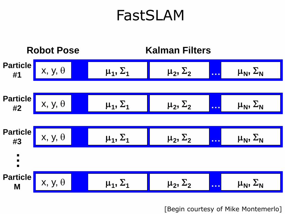
FastSLAM
Robot Pose Kalman Filters
m1, S1 m2, S2 mN, SN … x, y, q
m1, S1 m2, S2 mN, SN … x, y, q Particle
#1
m1, S1 m2, S2 mN, SN … x, y, q Particle
#2
m1, S1 m2, S2 mN, SN … x, y, q Particle
#3
Particle
M
…
[Begin courtesy of Mike Montemerlo]

FastSLAM Algorithm O(MN)
• Sample a new robot pose for each particle – xk = g(xk-1, uk) + v
– add this to trajectory giving x1:k
• Update the landmark EKFs in each particle – We have a ``known’’ (estimate) trajectory; run EKFs for each
landmark
• Calculate an importance weight (difference between actual observation, yk, and expected observation, with covariance Z)
• Resample particle set
knkkn
T
knk
kn
k yyYyyY
w ,
1
,,
,
ˆˆ2
1exp
2
1

SLAM Data Association
Angle increment = 0.00436940183863
Range1=[6.0000, 5.9996, 5.9985, …, 1.8759, 1.8771, 1.8784, …, 3.0107, 3.0284, 3.0447]
Range2=[2.0254, 2.0294, 2.0347, …, 2.0254, 2.0294, 2.0347, …, 6.0000, 6.0000, 6.0000]
Index2= [ 0 1 2 … 302 303 304 … 717 718 719 ]
Index1= [ 0 1 2 ... 532 533 534 … 717 718 719 ]

SLAM Data Association
• In practice we use a variable nk to associate each measurement to a landmark number (id#)
– For example n3 = 8 means that measurement at time k=3, y3, is associated with the landmark #8
• How do we get this nk?
),ˆ,ˆ,,|(maxargˆ
111 kkkkkkn
k uxnynyPnk
This is a “Maximum Likelihood” estimator.

FastSLAM Data Association
• In FastSLAM, each landmark is estimated with an EKF and the likelihood can be estimated from the EKF “innovation”
Robot Pose Kalman Filters
m1, S1 m2, S2 mN, SN … x, y, q
m1, S1 m2, S2 mN, SN … x, y, q Particle
#1
m1, S1 m2, S2 mN, SN … x, y, q Particle
#2
m1, S1 m2, S2 mN, SN … x, y, q Particle
#3
Particle
M
…
knkkn
T
knk
kn
kkkkk yyYyyY
uxnyyP ,
1
,,
,
111ˆˆ
2
1exp
2
1),ˆ,ˆ,|(
kny ,ˆ
ky
If the likelihood falls below a threshold, a new landmark is added

Tree of Landmarks
• FastSLAM complexity is log(MN) – M number of particles – N number of landmarks
• When we resample (with replacement) the same particle may be duplicated several times – Copying is linear in the size
of the map – Most of the landmarks
remain unchanged during a map update (only the visible landmarks are updated) From Montemerlo 2003
Robot Pose Kalman Filters
m1, S1 m2, S2 mN, SN … x, y, q
m1, S1 m2, S2 mN, SN … x, y, q Particle
#1
m1, S1 m2, S2 mN, SN … x, y, q Particle
#2
m1, S1 m2, S2 mN, SN … x, y, q Particle
#3
Particle
M
…
Robot Pose Kalman Filters
m1, S1 m2, S2 mN, SN …
x, y, q
m1, S1 m2, S2 mN, SN …
x, y, q Particle
#1
m1, S1 m2, S2 mN, SN …
x, y, q Particle
#2
m1, S1 m2, S2 mN, SN …
x, y, q Particle
#3
Particle
M
…
Robot Pose Kalman Filters
m1, S1 m2, S2 mN, SN …
x, y, q
m1, S1 m2, S2 mN, SN …
x, y, q Particle
#1
m1, S1 m2, S2 mN, SN …
x, y, q Particle
#2
m1, S1 m2, S2 mN, SN …
x, y, q Particle
#3
Particle
M …

Tree of Landmarks
• Use a tree of landmarks that is shared between particles
• If the tree is balanced then accessing a landmark takes log(N) and FastSLAM runs in log(M logN)
Balanced binary tree with 8 landmarks
[Courtesy of Mike Montemerlo]
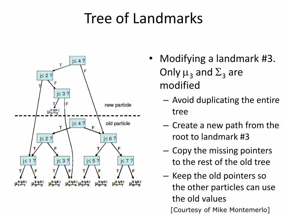
Tree of Landmarks
• Modifying a landmark #3. Only m3 and S3 are modified
– Avoid duplicating the entire tree
– Create a new path from the root to landmark #3
– Copy the missing pointers to the rest of the old tree
– Keep the old pointers so the other particles can use the old values
[Courtesy of Mike Montemerlo]

FastSLAM: Victoria Park Results
• 4 km traverse
• 100 particles
• GPS ground truth
• Uses negative evidence to remove spurious landmarks
• Uneven terrain
[Courtesy of Mike Montemerlo]

FastSLAM: Victoria Park Results
[End courtesy of Mike Montemerlo]
100 meters away from it’s true position
100 particles RMS error over 4km is ~4m

Grid-Based FastSLAM (occupancy grid)
map of particle 1 map of particle 3
map of particle 2
3 particles
Each particle must carry its entire map
[Courtesy of Mike Montemerlo]

FastSLAM Example
• 500 particles
• 28mx28m
• Length of trajectory 491m
• Map resolution 10cm

Closing the Loop
• Recognize a previously landmark
• Typically SLAM will drift, after a long drive the position and landmarks will be off
• Once an previously located object is seen – Make the correction – Propagate the correction
back – Uncertainties collapse
• With great powers comes great responsibility
• Uncertainty is not a “bad” thing
BEFORE
AFTER
Start at “you are here”
(no uncertainty) When the loop is
Close you are “back here”
[Newman 2005]
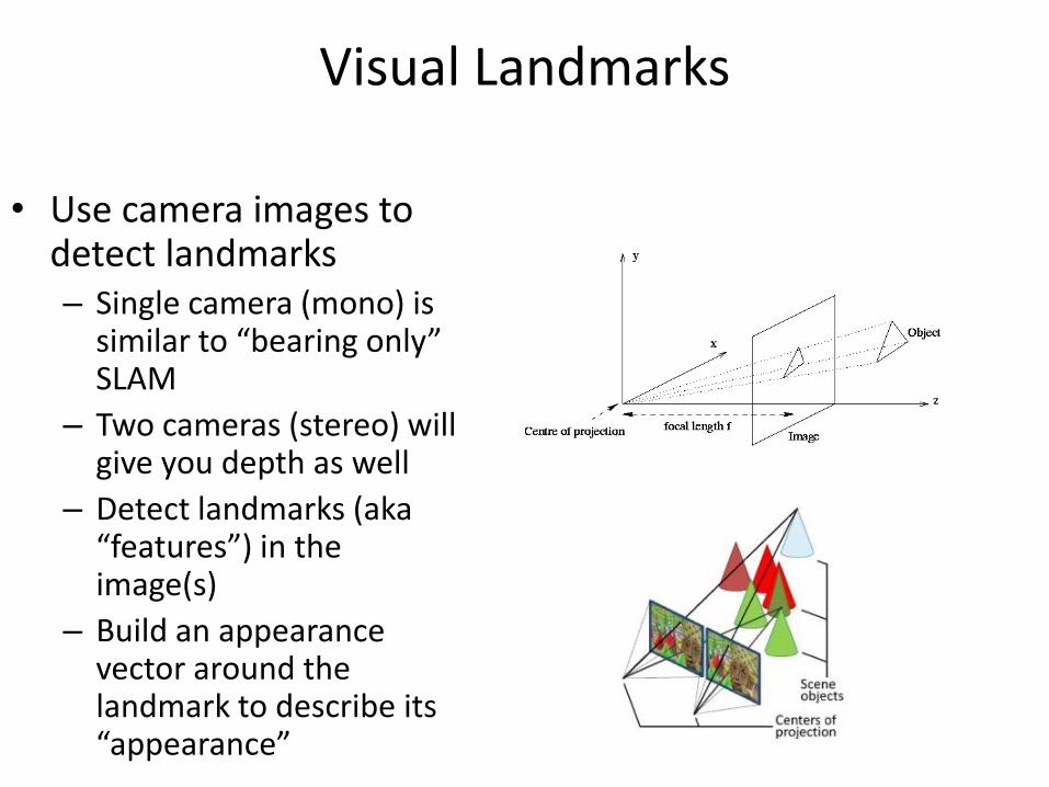
Visual Landmarks
• Use camera images to detect landmarks – Single camera (mono) is
similar to “bearing only” SLAM
– Two cameras (stereo) will give you depth as well
– Detect landmarks (aka “features”) in the image(s)
– Build an appearance vector around the landmark to describe its “appearance”

Visual Landmarks
Landmarks have a scale and orientation
Extract landmarks and their descriptors from two images. Then match the descriptors

Visual SLAM
SIFT landmarks from stereo camera Disparities are indicated by lines
Bird’s eye view of the 3D SIFT map Se, Lowe and Little 2005

RGBD SLAM (Red Green Blue Depth)
• Use camera and depth
• Provide a dense point cloud

RGBD SLAM
• Build dense, 3D, colored maps
• Lots of data so maps are usually small (small rooms or scanning objects)
• Use 3D data for localization
• Associate visual landmarks to 3D coordinates

Mapping Algorithms - Comparison SLAM
(Kalman)
EM ML* FastSLAM
Output Posterior ML/MAP ML/MAP Posterior
Convergence Strong Weak? No Stong
Local minima No Yes Yes No
Real time Yes No Yes Yes
Odom. Error Unbounded Unbounded Unbounded Unbounded
Sensor Noise Gaussian Any Any Any
# Features 103 >103
Feature uniq Yes No ~No Yes
Raw data No Yes Yes No

Localization and Mapping Summary • There are several methods for localization and mapping;
two dominant are – Kalman filter
• fast and efficient; very well understood • local convergence • strong assumptions
– Hypothesis-based methods (particle filters/Monte Carlo methods) • not as fast or efficient; not as well understood • global convergence • very weak assumptions
• The best methods today are hybrids – use hypotheses as necessary – use KF-like techniques whenever possible
• The largest revolution in mapping and localization has been data:“It’s all in the likelihood function” – laser scanners have really revolutionized the trade – vision is next?